A Framework for Correcting Ionospheric Artifacts and Atmospheric Effects to Generate High Accuracy InSAR DEM

1
The School of Geosciences and Info-Physics, Central South University, Changsha 410083, China
2
The School of Key Laboratory for Digital Dongting Lake Basin of Hunan Province & College of Science, Central South University of Forestry and Technology, Changsha 410018, China
*
Author to whom correspondence should be addressed.
Remote Sens. 2020, 12(2), 318; https://0-doi-org.brum.beds.ac.uk/10.3390/rs12020318
Submission received: 3 December 2019
/
Revised: 4 January 2020
/
Accepted: 15 January 2020
/
Published: 18 January 2020
(This article belongs to the Special Issue SAR Interferometry: Methods and Applications for Earth Science and Environmental Monitoring)
Abstract
:Repeat-pass interferometric synthetic aperture radar is a well-established technology for generating digital elevation models (DEMs). However, the interferogram usually has ionospheric and atmospheric effects, which reduces the DEM accuracy. In this paper, by introducing dual-polarization interferograms, a new approach is proposed to mitigate the ionospheric and atmospheric errors of the interferometric synthetic aperture radar (InSAR) data. The proposed method consists of two parts. First, the range split-spectrum method is applied to compensate for the ionospheric artifacts. Then, a multiresolution correlation analysis between dual-polarization InSAR interferograms is employed to remove the identical atmospheric phases, since the atmospheric delay is independent of SAR polarizations. The corrected interferogram can be used for DEM extraction. Validation experiments, using the ALOS-1 PALSAR interferometric pairs covering the study areas in Hawaii and Lebanon of the U.S.A., show that the proposed method can effectively reduce the ionospheric artifacts and atmospheric effects, and improve the accuracy of the InSAR-derived DEMs by 64.9% and 31.7% for the study sites in Hawaii and Lebanon of the U.S.A., respectively, compared with traditional correction methods. In addition, the assessment of the resulting DEMs also includes comparisons with the high-precision Ice, Cloud, and land Elevation Satellite-2 (ICESat-2) altimetry data. The results show that the selection of reference data will not affect the validation results.
1. Introduction
The interferometric synthetic aperture radar (InSAR) technology is a powerful remote sensing tool for generating digital elevation models (DEMs), owing to its day-and-night” and all-weather image acquisition capability, as well as its fine spatial resolution [1]. However, the various noise sources inherent in InSAR technology, such as ionospheric artifacts and atmospheric effects, greatly reduce the accuracy of topographic mapping. For the repeat-pass InSAR systems, the atmospheric effect is the dominant noise source. A spatial and temporal change of 20% in the relative humidity of the troposphere can result in an elevation error of about 100 m [2]. With the increasing number of low-frequency SAR systems scheduled for launches, such as the BIOMASS (P-Band) SAR satellite and the Tandem-L (L-Band) mission [3,4], the ionospheric delay becomes another major error source, which is inversely proportional to the frequency of the SAR system. Therefore, mitigating the ionospheric artifacts and atmospheric effects that are confused with the topographic phase is a great challenge in high-precision InSAR topographic mapping.
Over the past decades, a lot of efforts have been made to correct atmospheric effects [5,6,7]. Generally, there are three kinds of atmospheric correction methods. The first kind is based on the correlation between the atmospheric effects and the elevation [5]. These methods are simple and direct, but the correction accuracy is low. This is primarily attributed to the fact that the atmospheric effect is usually closely correlated with the elevation. The second kind of method needs auxiliary data, such as water vapor data and GPS data [6]. However, the water vapor data exactly corresponding to the SAR acquisition date and spatial coverage are not always available. The third family of methods estimates the atmospheric phase from multitemporal interferograms covering the same region [7]. The performance of this approach is dependent on the number of interferograms, so a large number of interferometric pairs are essential to obtain a reliable spatiotemporal analysis.
The latter two kinds of methods depend on the availability of auxiliary data or the number of SAR images, so they have very limited applications. A new method for atmospheric correction, which adopts a wavelet decomposition-based correlation analysis between interferograms in different polarizations to mitigate the atmosphere effects, was proposed [8]. Later, the moving window correlation analysis in this method was replaced by integral linear regression, so that the correlation analysis could identify the atmospheric effect more accurately [9] since the atmospheric phase could be correlated with the nonatmospheric phase in some areas. The method works well for eliminating atmospheric effects, but it cannot remove ionospheric artifacts and even atmospheric effects if they are mixed with ionospheric artifacts. However, how to correct the atmospheric and ionospheric error is of great concern for the long-wavelength (L-Band or P-Band) SAR systems [10].
The main objective of this paper is to propose a step-by-step correction method for the ionospheric artifacts and atmospheric effects in the repeat-pass InSAR topographic measurements. In Section 2, the phase components of different polarimetric interferograms are briefly reviewed, and the step-by-step correction is then elaborated. In Section 3, we validate the proposed method using the ALOS-1 PALSAR interferometric pairs of the study sites in Hawaii and Lebanon of the U.S.A. The generated DEMs are compared with the high precision TanDEM-X DEM. A discussion about the proposed method is presented in Section 4, and some conclusions are drawn in Section 5.
2. Methodology
2.1. Phase Components in the Dual-Polarization Interferograms
The InSAR phase is a superposition of different phase components, including the topographic phase , the flat-earth phase , the orbit error phase , the atmospheric and ionospheric delay phases , the surface deformation , and the noise phase :
where the superscript represents the selected polarimetric channel. In this equation, is the only useful information for deriving the high-precision DEM. The rest of the phases should be removed. The flat-earth phase can be calculated by orbit parameters. The orbit error phase caused by imprecise orbit parameters can be removed by a polynomial fitting model incorporating the elevation information [11]. can be ignored when an InSAR pair from a short temporal baseline is used [5]. is mainly caused by the thermal noise of the SAR sensor, as well as the decorrelation noise between two SAR acquisitions. Its impacts can be reduced through interferogram filtering [12]. and are caused by the spatial and temporal variations of the free electron numbers in the ionosphere and of the water vapor in the troposphere between the image acquisition interval, respectively. However, these two phases cannot be removed by a simple model and are the major error sources for InSAR DEM generation.
The ionosphere has two impacts on a traversing radar signal. First, a phase advance of the carrier will be induced, which is related to the density of the free electrons along the two-way wave path. This impact is polarization-independent. The ionospheric phase component can be calculated by [13]
where is the center frequency of the SAR signal; is the speed of light in vacuum; is the differential total electron content (TEC) between the master and slave image acquisition time along the light-of-sight (LOS) direction; and is a constant with the value of .
Second, there is the rotation of the polarization angle, which is also known as the Faraday rotation. Although the ionospheric artifact induced by the Faraday rotation is polarization-dependent, its contribution to the interferometric phase is small and can be ignored in most cases [13]. Therefore, it is reasonable to assume that different polarimetric interferograms contain fairly similar ionospheric phases. Moreover, the ionospheric phase is superimposed on the interferograms and usually shows as long-wavelength artifacts that are similar to the orbit error phase, which cannot be removed by the polynomial fitting model [14]. Within the short synthetic aperture time of SAR data, different polarimetric radio waves travel through the same atmospheric components, so that different polarimetric interferograms contain the same atmospheric phases. In summary, the atmospheric effect is polarization-independent, which provides us with a new idea to estimate and remove the atmospheric effects [8,9].
If the ionospheric effects caused by the Faraday rotation are not considered, both the ionospheric phases and atmospheric phases are polarization-independent. As a result, it is difficult to distinguish and correct the ionospheric artifacts and atmospheric effects based on the spatial characteristics of the interferometric phases [8,9], and even the orbit error phases cannot be corrected effectively. Therefore, we proposed a step-by-step correction approach to remove the ionospheric artifacts and atmospheric effects in interferograms. The proposed method adopts the range split-spectrum (RSS) method (described in Section 2.2) and the multi-resolution weighted correlation analysis (MRWCA) method (described in Section 2.3) to remove the ionospheric and atmospheric effects, respectively. The corrected interferograms can be used for DEM extraction.
2.2. Estimation of the Ionospheric Phase Component
According to Equation (2), the ionospheric phase is inversely related to the SAR frequency, while the other phase components are linearly related to the SAR frequency. So Equation (1) can be simplified as
where is the nondispersive phase component. Then, the ionosphere-related phase can be separated by the RSS technique through the following three steps:
- Step1:
- Coregistration of the master and slave images;
- Step2:
- Generating the single look complex (SLC) images of higher and lower spectral sub-bands by band-pass filtering.
- Step3:
- Estimation of ionospheric phase.
After Step1 and Step2, two sub-band interferograms can be obtained, which can be described as:
where and stand for the interferometric phases of the lower and higher spectral sub-bands. is the center frequency of the full-band radar range spectrum. and indicate the center frequencies of the lower sub-band and higher sub-band, respectively. Then, the dispersive phase and non-dispersive phase component can be estimated by
According to Equation (5), the ionospheric phase is a linear combination of the interferometric phases of the lower and higher spectral sub-bands and can be expressed as
where and are the constants associated with the spectrum of SAR data (for the ALOS-1 PALSAR FBD mode, ) [15]. Thus, a small phase noise will be amplified by the relatively large scaling factor, which will have a serious impact on the estimation of ionospheric phase. To improve the performance of the RSS method, the amplified phase noise should be suppressed by steps including spatial filtering, outlier removal processing, and phase unwrapping error correction [13].
2.3. Estimation of the Atmospheric Phase Component
Using the RSS technique, we can obtain the corrected differential interferograms (D-Infs) by removing the estimated ionospheric phase. If the dual-polarization SAR data are available, we have
where and are two selected polarization modes. is the residual topographic phase caused by the height error of DEM. is the polarization-related noise phase. Since the dual-polarization (or multi-polarization) InSAR data pairs share common orbit parameters, different polarimetric interferograms contain the same orbit error, which can be removed by the polynomial fitting model. Note that two different external DEMs are introduced to simulate the topographic phases for different polarimetric interferograms, so the final D-Infs contain different residual topographic phases. The D-Infs can be expressed as
According to Equation (8), the atmospheric phase is the only identical phase component in the obtained D-Infs. The MRWCA method can then be used to estimate the identical atmospheric phase.
2.4. The Overall Workflow of the Proposed Method
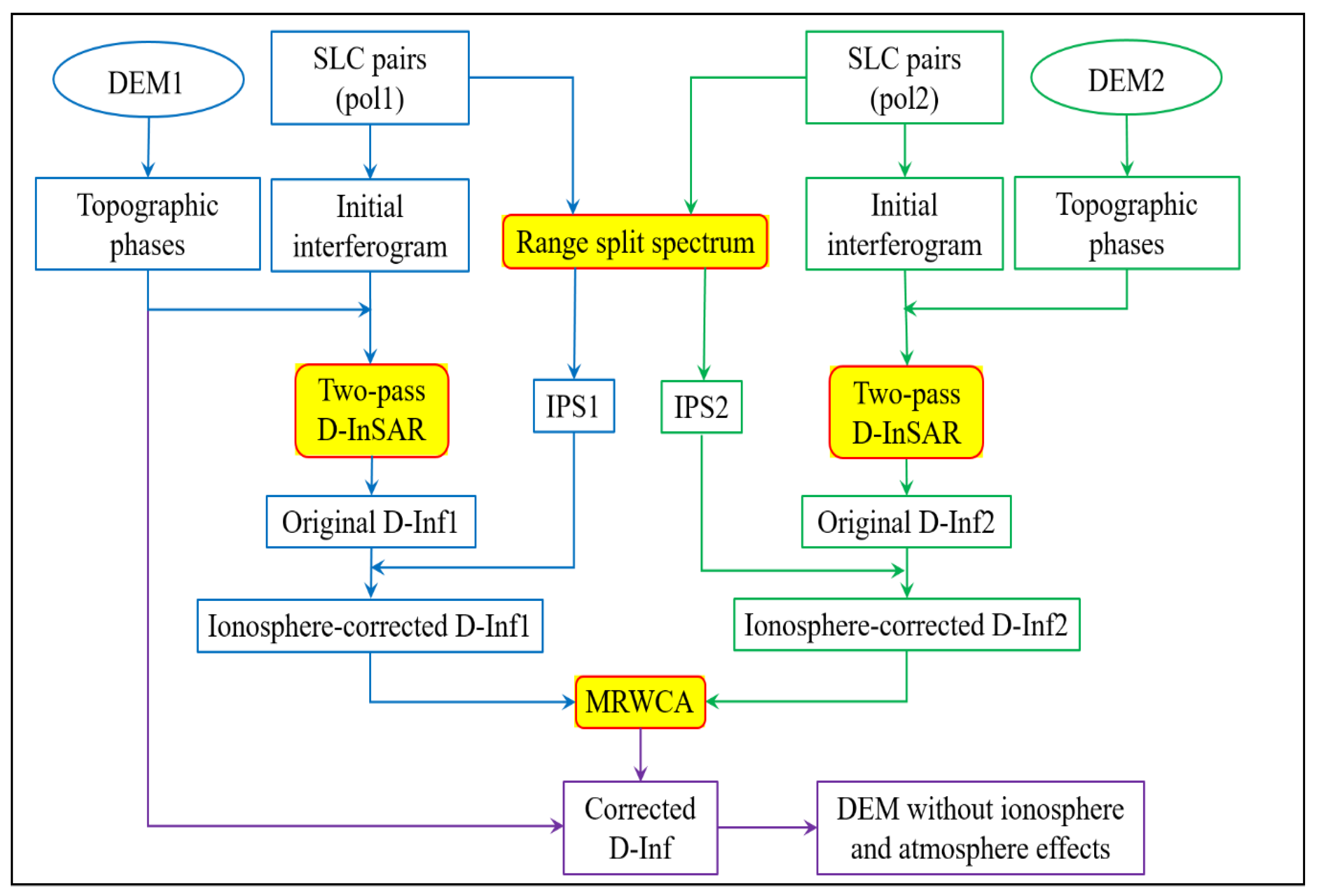
The overall workflow of the proposed method includes four main steps, as summarized in Figure 1. The first step is to generate the original D-Infs by the two-pass differential interferometry technique. This step can remove the polarization-independent phase components, including the flat-earth phase and the topographic phase. The RSS method is then utilized to estimate the ionospheric phase. After removing the estimated ionospheric phase from the original D-Infs, the ionosphere-corrected D-Infs can be obtained. Note that ionospheric phase correction should be done before removing the orbit error phase by the polynomial fitting model because the ionospheric phase will have impacts on the removal of the orbit error phases. The MRWCA method is subsequently adopted to detect the common atmospheric phases contained in different polarimetric interferograms [9]. Finally, we generate the corrected D-Infs by subtracting the atmospheric phases.
3. Case Studies
3.1. Hawaii Test Site
3.1.1. Test Area and Datasets
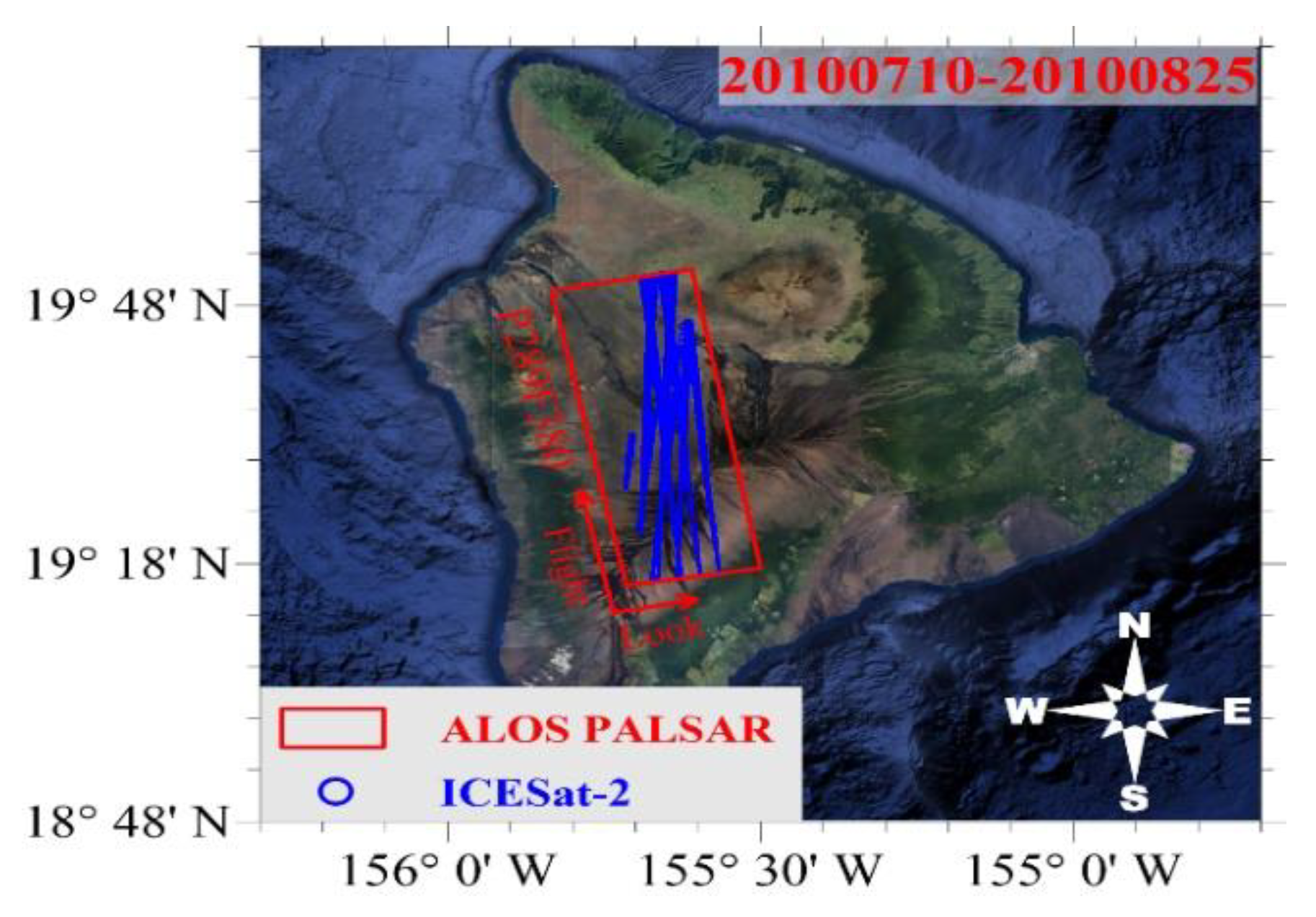
The selected SAR data over Hawaii, U.S.A., were acquired by the Advanced Land Observing Satellite-1 (ALOS-1) Phased Array-type L-Band Synthetic Aperture Radar (PALSAR) system on 10 July and 25 August 2010, with a coverage area of about 55 × 15 km, Polarimetry (PLR) mode, and an initial resolution of azimuth × range = 3.5 × 9.3 m. Figure 2 displays the footprint of the two SAR images (red rectangle) and the distribution of the ICESat-2 data (blue point). The ICESat-2 data were used to further validate the obtained DEM in Section 4.1.
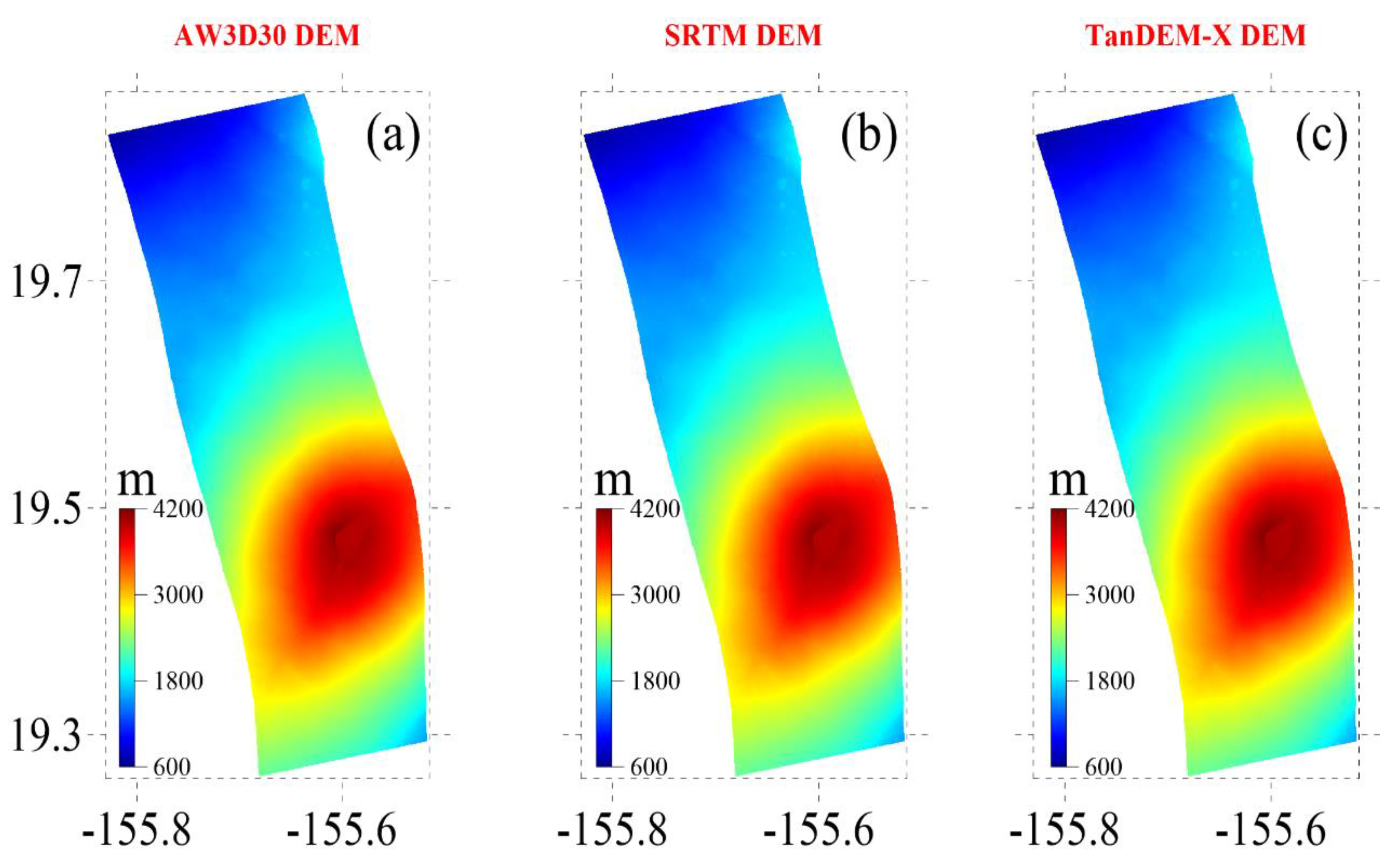
Due to the lack of the ASTER GDEM in the study area, we selected the ALOS World 3D—30 m (AW3D30) DEM [16] and the SRTM DEM [17] to remove the main topographic phases of the different polarimetric interferograms. In addition, the TanDEM-X DEM was used for validation [18,19,20]. The specific characteristics of the DEMs are shown in Figure 3a–c.
3.1.2. Step-by-Step Correction of Ionospheric Artifacts and Atmospheric Effects
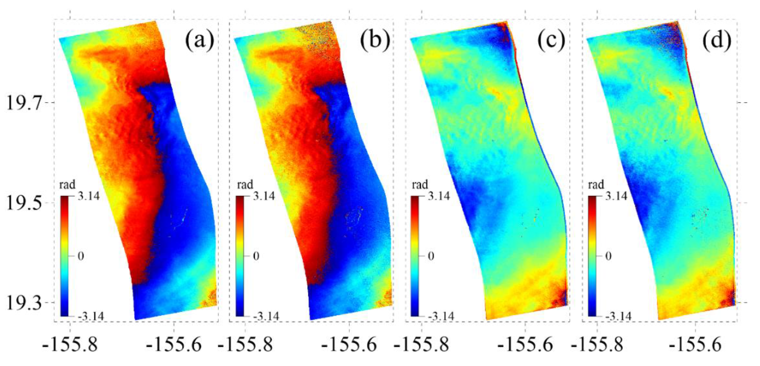
We applied the proposed method to remove the ionospheric artifacts and atmospheric effects. The selected interferometric pairs in different polarizations (HH and HV) were processed by a multi-look operation of 10 pixels in the azimuth direction and 2 pixels in the range direction to form D-Infs with a final resolution of 30 × 30 m. The orbit parameters and the two DEMs (i.e., the 1 arc-second AW3D30 DEM and the SRTM DEM) were then used to simulate the topographic phases for the HH and HV interferograms. The D-Infs obtained in such a way have different residual topographic phase components. To suppress the noise, the interferograms were filtered by the Goldstein filtering method [21]. Subsequently, and the minimum cost flow (MCF) approach [22] was adopted for the phase unwrapping with a coherence threshold of 0.3. Figure 4a,b displays the obtained initial D-Infs where the phases are wrapped. Since the acquisition interval of the ALOS images is 46 days, we can assume that the D-Infs have no phase components caused by significant topography changes, so the main phase components are the ionospheric phase, the atmospheric phase, and the topographic error phase.
The RSS method was used to estimate the ionospheric phase, which was then removed from the initial D-Infs. The corrected results are shown in Figure 4c,d in which the ionospheric phases have been successfully removed. The remaining phase components are the orbit error phase, residual topographic phase, atmospheric phase, and random noise. The residual long-wavelength trend error is mainly attributed to the orbit error phase, which can be removed by the polynomial fitting model. Figure 5a,b show the D-Infs after the ionospheric phases and orbit error phases have been removed. Although this polynomial fitting model incorporating height information can absorb some topography-dependent atmospheric phase, many atmospheric phase signals remain in the corrected D-Infs. The MRWCA method was then adopted to estimate the identical atmospheric phase signals contained in Figure 5a,b. Finally, we obtained the corrected D-Infs after the correction of atmospheric effects, which are presented in Figure 5c,d. The corrected D-Infs are mainly composed of residual topographic phases.
3.1.3. Reconstruction and Quality Assessment of the InSAR DEM
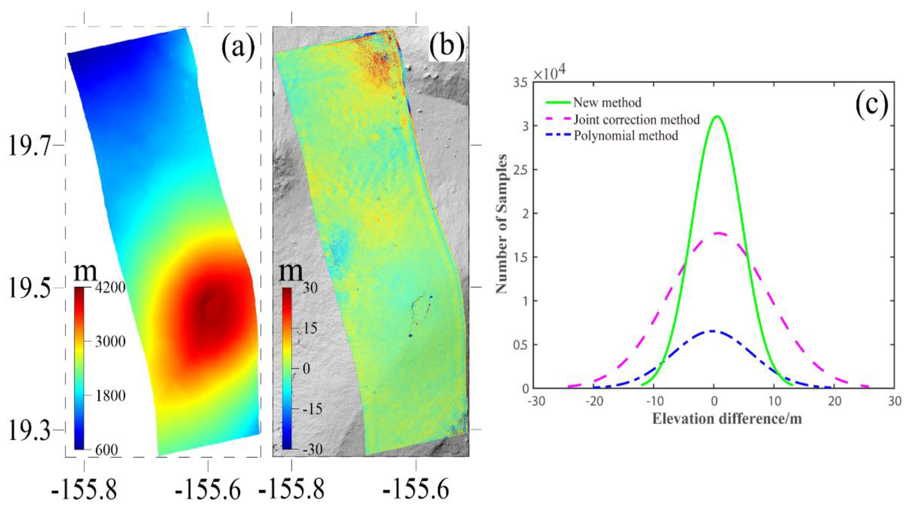
From the corrected HH interferogram, we generated the InSAR DEM, which was then geocoded and projected onto the World Geodetic System 1984 (WGS84) coordinate system, as shown in Figure 6a. The output grid spacing was set as 30 m in both the north and east directions. To assess the accuracy of the InSAR-derived DEM before and after the propagation delay error correction, the vertical accuracy of the DEM was compared with that of the reference DEM, which is the TanDEM-X DEM. Because the spatial resolution of the TanDEM-X DEM is 3 arc-seconds (roughly 90 m), we calculated an average value of the InSAR DEM with a window size of grid cells. The height difference map between the DEM derived by the proposed method and the reference DEM is shown in Figure 6b. The root mean squared error (RMSE) of the InSAR-derived DEM is 4.89 m.
For comparison, we also generated two DEMs from the HH-polarimetric interferograms that have been corrected by the joint correction method and the polynomial method. The joint correction method corrects the ionospheric phase by the RSS method first and then corrects the orbit error via the polynomial fitting model. The polynomial method corrects the two errors simultaneously using the polynomial fitting model. The corresponding histograms of the elevation differences with respect to TanDEM-X DEM are shown in Figure 6c. The RMSE of the DEM generated by the joint correction method is 10.28 m, and that of the DEM derived by the Polynomial method is 13.95 m. These accuracies are much lower than that of the DEM obtained by the proposed method (RMSE = 4.89 m).
According to the above results, the polynomial fitting model can mitigate some phase components with long wavelength (e.g., ionospheric phases and orbit error phases), although it is designed for correcting the orbit error phase. However, the polynomial fitting model alone cannot mitigate both ionospheric artifacts and orbit error phases, so these errors should be corrected separately. The joint correction method can correct the orbit error phase and ionospheric phase. But the study area has significant atmospheric effects (see Figure 5a,b). The proposed method, which can remove the ionospheric and atmospheric phases, can obtain a more accurate DEM.
3.2. Lebanon Test Site
3.2.1. Test Area and Datasets
We selected a test site located in the city of Lebanon in the northwestern United States to further validate the performance of the proposed method. The selected dual-polarization (HH and HV) interferometric pair acquired by L-band ALOS-1 PALSAR sensors has a temporal interval of 46 days and a coverage of around 80 km × 75 km, as shown in Figure 7.
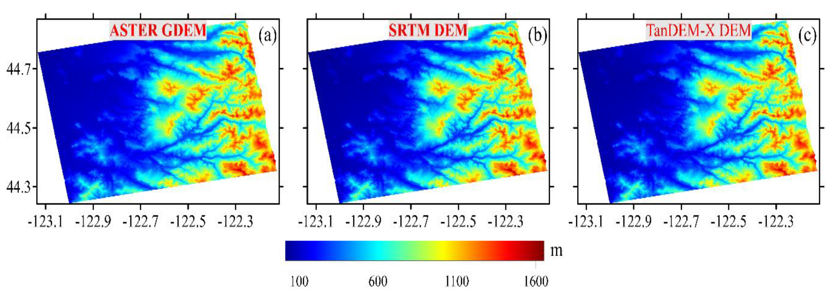
The ASTER GDEM and SRTM DEM with a resolution of 1 arc-second were used to simulate the topographic phase of the HH and HV interferograms, respectively (Figure 8a,b). The elevation of the study area varies from 12 to 1653 m above the mean sea level. The difference between SRTM and ASTER DEM has a global mean of 0.06 m with a standard deviation (STD) of 9.32 m. In addition, the TanDEM-X DEM with a 3 arc-second resolution (about 90 m) was used as the reference data for validation (Figure 8c).
3.2.2. Step-by-Step Correction of the Ionospheric Artifacts and Atmospheric Effects
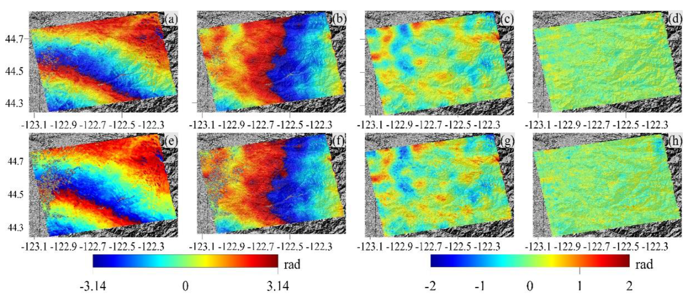
The selected InSAR data pairs in HH and HV polarizations were processed by the proposed method according to the workflow described in Section 2.4. The corresponding interferometric phase results are shown in Figure 9.
ASTER GDEM and SRTM DEM were adopted to calculate the topographic phase for the HH and HV interferograms, respectively, using the orbit parameters. Two initial D-Infs were obtained, as shown in Figure 9a,e, in which the ionospheric delay induces several distinctive fringes in the D-Infs.
The RSS technique was used to estimate the ionospheric phase, which was then removed from the original D-Infs. As the corrected results in Figure 9b,f show, there are no ionosphere-induced phases, but there are some residual phases, including the orbit error phase, atmospheric error phase, and residual topographic phase. Therefore, the long-wavelength residual phase is mainly attributed to the orbit error phase. In order to remove the orbit error phase, the polynomial fitting model was adopted. Figure 9c,g presents the residual phase maps after correcting the ionospheric artifacts by the RSS method and orbit error phase, which still have some atmospheric phase signals. This indicates that, although the polynomial fitting model incorporating height information could mitigate some of the topography-dependent atmospheric phases, the atmospheric phase signals are still conspicuous in the corrected D-Infs in Figure 9c,g.
Finally, the MRWCA method was used to estimate and remove the atmospheric phases contained in the corrected D-Infs. We could then obtain the final D-Infs, in which most of the positive and negative phase components caused by atmospheric effects have been mitigated by the MRWCA method. The residual topographic phase is the main remaining phase component (Figure 9d,h).
3.2.3. Reconstruction and Quality Assessment of the InSAR DEM
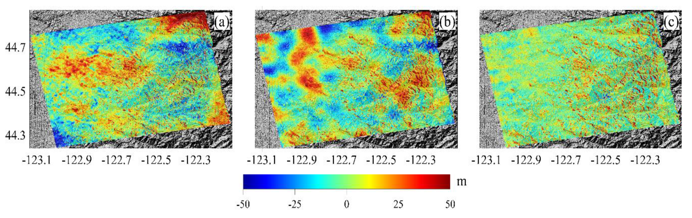
We generated DEMs from the HH interferograms corrected by the proposed approach, the polynomial method, and the joint correction method. These DEMs were compared with the TanDEM-X DEM for validation, and the elevation difference maps between InSAR DEM and Tandem-X DEM are displayed in Figure 10. The results show that the elevation difference of the proposed approach is significantly smaller than those of the other two methods, indicating that the proposed method can effectively remove the ionospheric artifacts and atmospheric effects on the interferograms, and thus can effectively improve the accuracy of InSAR topographic mapping. The RMSEs of the DEMs derived by the polynomial method, the joint correction method, and the proposed approach are 18.99 m, 18.57 m, and 12.96 m, respectively.
4. Discussion
4.1. Reference Elevation Data
In this study, the Tandem-X DEM was used to validate the DEM derived by the proposed method. However, the TanDEM-X DEM was generated from the X-band InSAR data, which has different penetration depth with the L-band SAR data in some areas, such as the vegetation and urban areas [23]. Although the elevation diversity caused by different penetration depths is not as large as that caused by other errors, such as residual orbit error, atmospheric error, and ionospheric artifact, the TanDEM-X DEM is not a proper reference for strict validation of the derived DEM. Hence, to eliminate the influence of single reference data on the validation results, high-precision altimetry data points from Ice, Cloud, and and Elevation Satellite-2 or ICESat-2 were adopted to further verify the accuracy of the derived DEM. These data are accurate enough to be used as ground control points (GCPs) for assessing the InSAR DEMs [24,25,26,27]. The blue dots in Figure 2 (3784 GCPs) and Figure 7 (7269 GCPs) are the ATL08 land data products collected by ICESat-2. We then calculated the elevation differences between the ICESat-2 data and the InSAR-derived DEMs. The elevation accuracies for different test sites and different correction methods are listed in Table 1.
For the study site in Hawaii, the largest RMSE corresponds to the DEM derived by the polynomial fitting method, which is 16.74 m. The second largest one, 14.29 m, is associated with the DEM derived by the joint correction method. However, the proposed method can effectively mitigate the effect of those errors on DEM and get an accuracy of RMSE = 7.10 m. We got similar results in the test site of Lebanon, U.S.A. However, the RMSE of the DEM derived by the proposed method is 17.79 m, which is significantly larger than that of the first test site. This could have resulted from many reasons: (1) besides the errors addressed in this paper, geometrical distortions can also significantly reduce the DEM accuracy, which has not been considered by the proposed method; (2) the ICESat-2 point distribution is too sparse to describe the DEM error well in spatial. Therefore, it is also not very reasonable to validate the DEM by the ICESat-2 data. Using other reference data (e.g., local or regional LiDAR-derived DEM) might help the validation of the DEM derived by the proposed method.
4.2. Ground Deformation
In this study, the ground deformation was not considered, because: (1) For DEM extraction, to secure good interferometric phase quality, interferometric pairs with short temporal baselines are preferred [5]. In such a case, the ground deformation is negligible in most regions, and the effect of deformation on the DEM extraction can be ignored. (2) If large ground deformations occur during InSAR data acquisition, the deformation signals cannot be removed by the RRS method, since the deformation signals are nondispersive [13,14]. However, the ground deformation signals can be recorded by InSAR data in different polarizations in the same or similar ways. If the deformation signals are identical in different polarimetric D-InSAR interferograms, the MRWCA method can remove the deformation signals together with the atmospheric phase [9]. However, when the D-InSAR interferograms have similar deformation signals, some deformation signals cannot be removed by the MRWCA method and will be converted into the topographic information. This problem still needs to be studied further in the future.
5. Conclusions
In this paper, an approach combing the RSS and MRWCA methods has been proposed to reduce the ionospheric artifacts and atmospheric effects on the polarimetric InSAR interferograms used for DEM generation. The performance of the proposed method has been validated by the L-Band ALOS-1 PALSAR InSAR pairs covering Hawaii and Lebanon of the U.S.A. For the Hawaii test site, the RMSE of the DEM generated by the proposed approach is 4.89 m with respect to the TanDEM-X DEM, which is smaller than those derived by the joint correction method (10.28 m) and polynomial method (13.95 m). For the second test site, the proposed method also has the highest accuracy, with RMSE = 12.96 m. Furthermore, the validation using the ICESat-2 altimetry data as the reference (described in Section 4.1) got similar results. According to these results, the following conclusions are drawn: (1) the proposed method is feasible and effective, and (2) it can improve the original MRWCA method and thus expands its application scopes.
The main advantage of the proposed method is that it can remove the ionospheric artifacts and atmospheric error phases from polarimetric InSAR data, without using any assumption or external auxiliary data. However, the decorrelation and phase unwrapping error are the two main problems affecting the performance of the proposed method. For DEM extraction, to secure good interferometric phase quality, interferometric pairs with short temporal baselines are usually selected. In such a case, the influences of the decorrelation and phase unwrapping error on the proposed method can be reduced. As far as the ionospheric correction is concerned, if the conventional RSS method cannot be adopted to estimate the ionospheric phase due to the low coherence, other correction methods can be used, such as the multiple sub-bands RSS method [14] or Faraday rotation method [28,29,30].
Up to the present, the proposed method is mainly used to correct ionospheric and atmospheric effects to extract high accuracy InSAR DEM. However, an extension of the proposed method to the field of D-InSAR is a topic worthy of further investigations. In order to solve this problem, it is important to analyze the character of the deformation signal. As far as the ionospheric correction is concerned, since the deformation signals are nondispersive, the deformation signals will not be removed by the RRS method [14]. However, to correct the atmospheric effects by the MRWCA method and retain the useful deformation information, it is crucial to research how to separate the deformation signals and then estimate the atmospheric phases in future work.
Author Contributions
Conceptualization, Z.L. and H.F.; methodology, Z.L.; software, H.F.; validation, Z.L., C.Z., J.Z., and T.Z.; formal analysis, Z.L., J.Z., and T.Z.; investigation, C.Z.; resources, J.Z.; data curation, J.Z. and H.F.; writing—original draft preparation, Z.L.; writing—review and editing, Z.L., H.F., and J.Z.; supervision, H.F.; project administration, C.Z. and J.Z.; funding acquisition, C.Z. and J.Z. All authors have read and agreed to the published version of the manuscript.
Funding
This work was supported in part by the National Natural Science Foundation of China under Grant 41604012, Grant 41904004, Grant 41531068, and Grant 41674009, and in part by the Young Elite Scientists Sponsorship Program by Hunan province of China under Grant 2018RS3093 and China Postdoctoral Science Foundation under Grant 2017M612604.
Acknowledgments
The authors would like to thank the Alaska Satellite Facility (ASF) for providing the ALOS-1 PALSAR data. The authors would further like to thank Wenhao Wu from the Hunan University of Science and Technology, Bochen Zhang from The Hong Kong Polytechnic University, and Wanpeng Feng from the Sun Yat-Sen University, for the helpful discussions on the range split-spectrum ionospheric correction method. In addition, ALOS AW3D30 data ©JAXA; 90-m TanDEM-X DEM data ©DLR; and ICESat-2 altimetry data were provided by National Snow & Ice Data Center (NSIDC).
Conflicts of Interest
The authors declare no conflict of interest.
References
- Madsen, S.N.; Zebker, H.; Martin, J. Topographic mapping using radar interferometry: Processing techniques. IEEE Trans. Geosci. Remote Sens. 1993, 31, 246–256. [Google Scholar] [CrossRef]
- Zebker, H.A.; Rosen, P.A.; Hensley, S. Atmospheric effects in interferometric synthetic aperture radar surface deformation and topographic maps. J. Geophys. Res. Solid Eaeth 1997, 102, 7547–7563. [Google Scholar] [CrossRef]
- Quegan, S.; Le Toan, T.; Chave, J.; Dall, J.; Exbrayat, J.F.; Minh, D.H.T.; Lomas, M.; D’Alessandro, M.M.; Paillou, P.; Rocca, F.; et al. The European Space Agency BIOMASS mission: Measuring forest above-ground biomass from space. Remote Sens. Environ. 2019, 227, 44–60. [Google Scholar] [CrossRef] [Green Version]
- Moreira, A.; Krieger, G.; Hajnsek, I.; Papathanassiou, K.; Younis, M.; Lopez-Dekker, F.; Huber, S.; Eineder, M.; Shimada, M.; Motohka, T.; et al. ALOS-Next/Tandem-L: A Highly Innovative SAR Mission for Global Observation of Dynamic Processes on the Earth’s Surface. In Proceedings of the IEEE International Geoscience and Remote Sensing Symposium, Milan, Italy, 26–31 July 2015; Volume 3, pp. 8–23. [Google Scholar]
- Liao, M.; Jiang, H.; Wang, Y.; Wang, T.; Zhang, L. Improved topographic mapping through high-resolution SAR interferometry with atmospheric effect removal. ISPRS J. Photogram. Remote Sens. 2013, 80, 72–79. [Google Scholar] [CrossRef]
- Li, Z.W.; Xu, W.B.; Feng, G.C.; Hu, J.; Wang, C.C.; Ding, X.L.; Zhu, J.J. Correcting atmospheric effects on InSAR with MERIS water vapour data and elevation-dependent interpolation model. Geophys. J. Int. 2012, 189, 898–910. [Google Scholar] [CrossRef] [Green Version]
- Ferretti, A.; Prati, C.; Rocca, F. Permanent scatterers in SAR interferometry. IEEE Trans. Geosci. Remote Sens. 2001, 39, 8–20. [Google Scholar] [CrossRef]
- Fu, H.Q.; Zhu, J.J.; Wang, C.C.; Zhao, R.; Xie, Q.H. Atmospheric Effect Correction for InSAR With Wavelet Decomposition-Based Correlation Analysis Between Multipolarization Interferograms. IEEE Trans. Geosci. Remote Sens. 2018, 56, 5614–5625. [Google Scholar] [CrossRef]
- Liu, Z.; Fu, H.; Zhu, J.; Zhou, C.; Zuo, T. Using Dual-Polarization Interferograms to Correct Atmospheric Effects for InSAR Topographic Mapping. Remote Sens. 2018, 10, 1310. [Google Scholar] [CrossRef] [Green Version]
- Quegan, S.; Lomas, M.; Papathanassiou, K.P.; Kim, J.S.; Tebaldini, S.; Giudici, D.; Scagliola, M.; Guccione, P.; Dall, J.; Dubois-Fenandez, P.; et al. Calibration Challenges for the Biomass P-Band SAR Instrument. In Proceedings of the IGARSS IEEE, Valencia, Spain, 22–27 July 2018; pp. 8575–8578. [Google Scholar]
- Liao, M.; Wang, T.; Lu, L.; Zhou, W.; Li, D. Reconstruction of DEMs from ERS-1/2 Tandem Data in Mountainous Area Facilitated by SRTM Data. IEEE Trans. Geosci. Remote Sens. 2007, 45, 2325–2335. [Google Scholar] [CrossRef]
- Goldstein, R.M.; Werner, C.L. Radar interferogram filtering for geophysical applications. Geophys. Res. Lett. 1998, 25, 4035–4038. [Google Scholar] [CrossRef] [Green Version]
- Gomba, G.; Parizzi, A.; De Zan, F.; Eineder, M.; Bamler, R. Toward Operational Compensation of Ionospheric Effects in SAR Interferograms: The Split-Spectrum Method. IEEE Trans. Geosci. Remote Sens. 2016, 54, 1446–1461. [Google Scholar] [CrossRef] [Green Version]
- Liao, H. Ionospheric Correction of Interferometric Sar Data with Application to the Cryospheric Sciences. Ph.D. Thesis, University of Alaska Fairbanks, Fairbanks, AK, USA, 2018. [Google Scholar]
- Wegmüller, U.; Werner, C.; Frey, O.; Magnard, C.; Strozzi, T. Reformulating the Split-Spectrum Method to Facilitate the Estimation and Compensation of the Ionospheric Phase in SAR Interferograms. Procedia Comput. Sci. 2018, 138, 318–325. [Google Scholar] [CrossRef]
- Tadono, T.; Tsutsui, K. Generation of High Resolution Global DSM from ALOS PRISM. ISPRS J. Photogramm. Remote Sens. 2014, 2, 243–248. [Google Scholar]
- Farr, T.G.; Rosen, P.A.; Caro, E.; Crippen, R.; Duren, R.; Hensley, S.; Kobrick, M.; Paller, M.; Rodriguez, E.; Roth, L.; et al. The Shuttle Radar Topography Mission. Rev. Geophys. 2007, 45, 1–33. [Google Scholar] [CrossRef] [Green Version]
- Rizzoli, P.; Martone, M.; Gonzalez, C.; Wecklich, C.; Tridon, D.B.; Bräutigam, B.; Bachmann, M.; Schulze, D.; Fritz, T.; Huber, M.; et al. Generation and performance assessment of the global TanDEM-X digital elevation model. ISPRS J. Photogramm. Remote Sens. 2017, 132, 119–139. [Google Scholar] [CrossRef] [Green Version]
- Gruber, A.; Wessel, B.; Huber, M.; Roth, A. Operational TanDEM-X DEM calibration and first validation results. ISPRS J. Photogramm. Remote Sens. 2012, 73, 39–49. [Google Scholar] [CrossRef]
- Grohmann, C.H. Evaluation of TanDEM-X DEMs on selected Brazilian sites: Comparison with SRTM, ASTER GDEM and ALOS AW3D30. Remote Sens. Environ. 2018, 212, 121–133. [Google Scholar] [CrossRef] [Green Version]
- Li, Z.W.; Ding, X.L.; Huang, C.; Zhu, J.J.; Chen, Y.L. Improved filtering parameter determination for the Goldstein radar interferogram filter. ISPRS J. Photogramm. Remote Sens. 2008, 63, 621–634. [Google Scholar] [CrossRef]
- Chen, C.W.; Zebker, H.A. Two-dimensional phase unwrapping with use of statistical models for cost function in nonlinear optimization. J. Opt. Soc. Am. A 2001, 18, 338–351. [Google Scholar] [CrossRef] [Green Version]
- Shiroma, G.H.X.; Macedo, K.A.C.D.; Wimmer, C.; Fernandes, D.; Barreto, T.L. Combining dual-band capability and polinsar technique for forest ground and canopy estimation. In Proceedings of the IGARSS 2014, Quebec City, QC, Canada, 13–18 July 2014. [Google Scholar]
- Neuenschwander, A.L.; Popescu, S.C.; Nelson, R.F.; Harding, D.; Pitts, K.L.; Robbins, J. ATLAS/ICESat-2 L3A Land and Vegetation Height; Version 2; National Snow and Ice Data Center: Boulder, CO, USA, 2019. [Google Scholar] [CrossRef]
- Neuenschwander, A.L.; Magruder, L.A. Canopy and terrain height retrievals with ICESat-2: A first look. Remote Sens. 2019, 11, 1721. [Google Scholar] [CrossRef] [Green Version]
- Neuenschwander, A.; Pitts, K. The ATL08 land and vegetation product for the ICESat-2 Mission. Remote Sens. Environ. 2019, 221, 247–259. [Google Scholar] [CrossRef]
- Smith, B.; Fricker, H.A.; Holschuh, N.; Gardner, A.S.; Adusumilli, S.; Brunt, K.M.; Csatho, B.; Harbeck, K.; Huth, A.; Neumann, T.; et al. Land ice height-retrieval algorithm for NASA’s ICESat-2 photon-counting laser altimeter. Remote Sens. Environ. 2019, 233, 111352. [Google Scholar] [CrossRef] [Green Version]
- Gomba, G.; De Zan, F. Bayesian Data Combination for the Estimation of Ionospheric Effects in SAR Interferograms. IEEE Trans. Geosci. Remote Sens. 2017, 55, 6582–6593. [Google Scholar] [CrossRef]
- Zhen, L.; Jung, H.S.; Zhong, L. Joint Correction of Ionosphere Noise and Orbital Error in L-Band SAR Interferometry of Interseismic Deformation in Southern California. IEEE Trans. Geosci. Remote Sens. 2014, 52, 3421–3427. [Google Scholar]
- Pi, X.; Freeman, A.; Chapman, B.; Rosen, P.; Li, Z. Imaging ionospheric inhomogeneities using spaceborne synthetic aperture radar. J. Geophys. Res. 2011, 116, A04303. [Google Scholar] [CrossRef]
Figure 1.
The workflow of the proposed method for correcting the ionospheric artifacts and atmospheric effects of interferograms and generating the interferometric synthetic aperture radar (InSAR) digital elevation model (DEM). IPS = ionosphere phase screen; D-Inf = differential interferogram.
Figure 1.
The workflow of the proposed method for correcting the ionospheric artifacts and atmospheric effects of interferograms and generating the interferometric synthetic aperture radar (InSAR) digital elevation model (DEM). IPS = ionosphere phase screen; D-Inf = differential interferogram.

Figure 2.
Coverage of the ALOS-1 PALSAR data and the spatial distribution of Ice, Cloud, and land Elevation Satellite-2 (ICESat-2) altimetry data over this study area. The optical image was downloaded from Google Earth.
Figure 2.
Coverage of the ALOS-1 PALSAR data and the spatial distribution of Ice, Cloud, and land Elevation Satellite-2 (ICESat-2) altimetry data over this study area. The optical image was downloaded from Google Earth.

Figure 3.
The DEM data used in this study. (a) AW3D30 DEM, (b) SRTM DEM and (c) TanDEM-X DEM.

Figure 4.
(a,b) are the initial D-Infs of the HH and HV polarizations, respectively. (c,d) are the D-Infs after ionospheric correction by the range split-spectrum method.
Figure 4.
(a,b) are the initial D-Infs of the HH and HV polarizations, respectively. (c,d) are the D-Infs after ionospheric correction by the range split-spectrum method.

Figure 5.
The unwrapped D-Infs of the HH and HV polarizations, corrected by the proposed method. (a,b) after the correction of ionospheric and orbit errors; and (c,d) after the atmospheric error correction.
Figure 5.
The unwrapped D-Infs of the HH and HV polarizations, corrected by the proposed method. (a,b) after the correction of ionospheric and orbit errors; and (c,d) after the atmospheric error correction.

Figure 6.
(a) The InSAR DEM generated from the corrected HH-polarization interferograms by the proposed method. (b) The elevation difference between InSAR DEM obtained by the proposed method and TanDEM-X DEM. (c) Histograms of the elevation difference between the InSAR-derived DEMs and the TanDEM-X DEM.

Figure 7.
The coverage of the ALOS-1 PALSAR images (red rectangle) and the distribution of the ICESat-2 data (blue dots). The optical image was downloaded from Google Earth.
Figure 7.
The coverage of the ALOS-1 PALSAR images (red rectangle) and the distribution of the ICESat-2 data (blue dots). The optical image was downloaded from Google Earth.

Figure 8.
(a) ASTER GDEM. (b) SRTM DEM. (c) TanDEM-X DEM.

Figure 9.
The original and corrected differential interferograms. The first row is the results of HH-polarization, and the second row represents the results of HV-polarization. (a,e): Original D-Infs. (b,f): D-Infs after correcting ionospheric artifacts. (c,g): D-Infs after removing orbit error phases. (d,h): D-Infs after correcting atmospheric phases. In addition (a,b,e,f) are the wrapped phases, while (c,d,g,h) are the unwrapped phases.

Figure 10.
The elevation difference between the reference DEM and the one obtained (a) by the polynomial method; (b) by the joint correction method; and (c) by the proposed method in this paper.
Figure 10.
The elevation difference between the reference DEM and the one obtained (a) by the polynomial method; (b) by the joint correction method; and (c) by the proposed method in this paper.


Table 1.
Performance of the InSAR DEMs with different correction methods at study sites Hawaii and Lebanon of the U.S.A.
Table 1.
Performance of the InSAR DEMs with different correction methods at study sites Hawaii and Lebanon of the U.S.A.
| Sites | ICESat-2 | Polynomial Method | Joint Correction Method | New Method |
|---|---|---|---|---|
| RMSE(m) | ||||
| Hawaii | 3784 | 16.74 | 14.29 | 7.10 |
| Lebanon | 7269 | 23.33 | 22.07 | 17.79 |
© 2020 by the authors. Licensee MDPI, Basel, Switzerland. This article is an open access article distributed under the terms and conditions of the Creative Commons Attribution (CC BY) license (http://creativecommons.org/licenses/by/4.0/).
Share and Cite
MDPI and ACS Style
Liu, Z.; Zhou, C.; Fu, H.; Zhu, J.; Zuo, T. A Framework for Correcting Ionospheric Artifacts and Atmospheric Effects to Generate High Accuracy InSAR DEM. Remote Sens. 2020, 12, 318. https://0-doi-org.brum.beds.ac.uk/10.3390/rs12020318
AMA Style
Liu Z, Zhou C, Fu H, Zhu J, Zuo T. A Framework for Correcting Ionospheric Artifacts and Atmospheric Effects to Generate High Accuracy InSAR DEM. Remote Sensing. 2020; 12(2):318. https://0-doi-org.brum.beds.ac.uk/10.3390/rs12020318
Chicago/Turabian StyleLiu, Zhiwei, Cui Zhou, Haiqiang Fu, Jianjun Zhu, and Tingying Zuo. 2020. "A Framework for Correcting Ionospheric Artifacts and Atmospheric Effects to Generate High Accuracy InSAR DEM" Remote Sensing 12, no. 2: 318. https://0-doi-org.brum.beds.ac.uk/10.3390/rs12020318
Note that from the first issue of 2016, this journal uses article numbers instead of page numbers. See further details here.