A Multi-Year Evaluation of Doppler Lidar Wind-Profile Observations in the Arctic


Meteorological Research Division, Environment and Climate Change Canada, Toronto, ON M3H-5T4, Canada
*
Author to whom correspondence should be addressed.
Remote Sens. 2020, 12(2), 323; https://0-doi-org.brum.beds.ac.uk/10.3390/rs12020323
Submission received: 3 December 2019
/
Revised: 6 January 2020
/
Accepted: 10 January 2020
/
Published: 18 January 2020
(This article belongs to the Special Issue Advances in Atmospheric Remote Sensing with Lidar)
Abstract
:Doppler light detection and ranging (lidar) wind profilers have proven their capability to measure vertical wind profiles with an accuracy comparable to anemometers and radiosondes. However, most of these comparisons were performed over short time periods or at mid-latitudes. This study presents a multi-year assessment of the accuracy of Doppler lidar wind-profile measurements in the Arctic by comparing them with coincident radiosonde observations, and excellent agreement was observed. The suitability of the Doppler lidar for verification case studies of operational numerical weather prediction (NWP) models during the World Meteorological Organization’s Year of Polar Prediction is also demonstrated, by using Environment and Climate Change Canada’s (ECCC) global environmental multiscale model (GEM-2.5 km and GEM-10 km). Since 2016, identical scanning Doppler lidars were deployed at two supersites commissioned by ECCC as part of the Canadian Arctic Weather Science project. The supersites are located in Iqaluit (64°N, 69°W) and Whitehorse (61°N, 135°W) with a third Halo Doppler lidar located in Squamish (50°N, 123°W). Two lidar wind-profile measurement methodologies were investigated; the velocity-azimuth display method exhibited a smaller average bias (−0.27 ± 0.02 m/s) than the Doppler beam-swinging method (–0.46 ± 0.02 m/s) compared to the sonde. Comparisons to ECCC’s NWP models indicate good agreement, more so during the summer months, with an average bias < 0.71 m/s for the higher-resolution (GEM-2.5 km) ECCC models at Iqaluit. Larger biases were found in the mountainous terrain of Whitehorse and Squamish, likely due to difficulties in the model’s ability to resolve the topography. This provides evidence in favor of using high temporal resolution lidar wind-profile measurements to complement radiosonde observations and for NWP model verification and process studies.
1. Introduction
Accurate and reliable measurements of the vertical wind profile are an essential meteorological observation, particularly with respect to numerical weather prediction (NWP), climate modelling, air-quality monitoring and forecasting, and generation of energy forecasting. Operational vertical wind-profile measurements are dominated by global radiosonde observations and, to a lesser extent, radar wind profilers (RWP). However, with recent advancements in light detection and ranging (lidar)-based technologies over the past few decades, comprehensive high spatial- and temporal-resolution profiling of winds within the boundary layer has become increasingly common.
Commercially available Doppler lidar wind profilers have proven their capability of measuring the wind speed and turbulence intensity with an accuracy comparable to the well-established cup anemometers over non-complex terrain [1,2]. Doppler lidars have several advantages over radiosondes and RWPs: (1) the lidar’s narrow beam removes the issue of ground clutter, making measurements possible in complex terrain [3,4,5,6,7,8]; (2) measurements can be taken in urban areas where radiosondes cannot be launched; (3) observations can be conducted during high surface winds when radiosondes cannot be launched; (4) they are easily deployable and can be mobile [7]; (5) they can take measurements below the height of the first range gate of most RWPs; (6) observations exhibit no measurement drift; and (7) the cost of a lidar system is typically less than a RWP while offering higher-resolution data. The most notable disadvantage of most Doppler lidars is their decreased vertical range, which is usually limited to the boundary layer height. It should be noted that more powerful Doppler lidars, though rare, are capable of conducting measurements above the boundary layer [9].
Previous studies comparing observations from Doppler lidars, anemometers, radiosondes, and RWPs have generally shown good agreement with biases in the range of ~0.5–0.7 m/s and R2 values >0.85 [10,11,12,13,14,15,16,17,18,19]. However, most of these comparisons were performed over shorter time periods lasting less than a year and, with the exception of Newsom et al. [19], Achtert et al. [17], and Mizutani et al. [10], took place at mid-latitudes. It is vital to assess the accuracy of the Doppler lidar wind profiles in other climates such as the Arctic where operational conditions are extreme and the boundary layer height and aerosol concentrations are lower than at mid latitudes. These atmospheric conditions typically cause a reduced backscatter signal and lower vertical range for the lidar, presenting a ‘worst-case’ scenario in terms of its performance.
Environment and Climate Change Canada (ECCC) commissioned two supersites in the Arctic and sub-Arctic to provide automated and continuous observations of altitude-resolved winds, water vapour, clouds and aerosols, visibility, radiation fluxes, and precipitation as part of the Canadian Arctic Weather Science (CAWS) project [20]. The supersites are located in Iqaluit, NU (64°N, 69°W) and Whitehorse, YT (61°N, 135°W). A third, smaller ECCC site in Squamish, BC (50°N, 123°W) was also equipped with a Doppler lidar.
Iqaluit and Whitehorse were designated supersites for the World Meteorological Organization’s (WMO) Year of Polar Prediction (YOPP) project (core phase: mid 2017 to mid 2019) for international NWP forecast model inter-comparison and verification [21]. The representation of the structure and physical processes governing Arctic boundary layers is still a challenge in NWP systems due to issues with numerical stability. Moreover, wind observations are among the highest-ranked contributors to NWP model forecast error [22,23]. Therefore, it is essential to perform enhanced validation of NWP model winds within the boundary layer in the Arctic environment, and to investigate the potential of assimilating additional wind observations that could reduce this forecast error [9,24]. To address these needs, international NWP modeling centres, including ECCC, provided high-frequency model output data at and around each supersite during the YOPP, enabling enhanced model verification, inter-comparisons, and process studies to be conducted.
In this study, comparisons between the Doppler lidar and radiosonde were performed at Iqaluit during the pre-YOPP period to assess the accuracy of the Doppler lidar wind-profile observations. Once the lidar-sonde agreement was characterized, comparisons between the Doppler lidar and ECCC NWP model observations were performed at three sites to evaluate the models’ performance and determine the models’ biases relative to the lidar at high temporal resolution. Section 2 describes the Iqaluit and Whitehorse supersites, the Squamish site, and the instrumentation, including a description of the two types of Doppler lidar scans utilized to measure the vertical wind profile. Section 3 provides a discussion of results on the comparisons between the Doppler lidar and radiosonde observations at Iqaluit, describes the ECCC NWP models used to perform the verification case studies, and provides initial results on the comparisons between the Doppler lidar and the ECCC NWP models at all three sites. Conclusions and future work are provided in Section 4.
2. Materials and Methods
2.1. Iqaluit, Whitehorse, and Squamish Sites
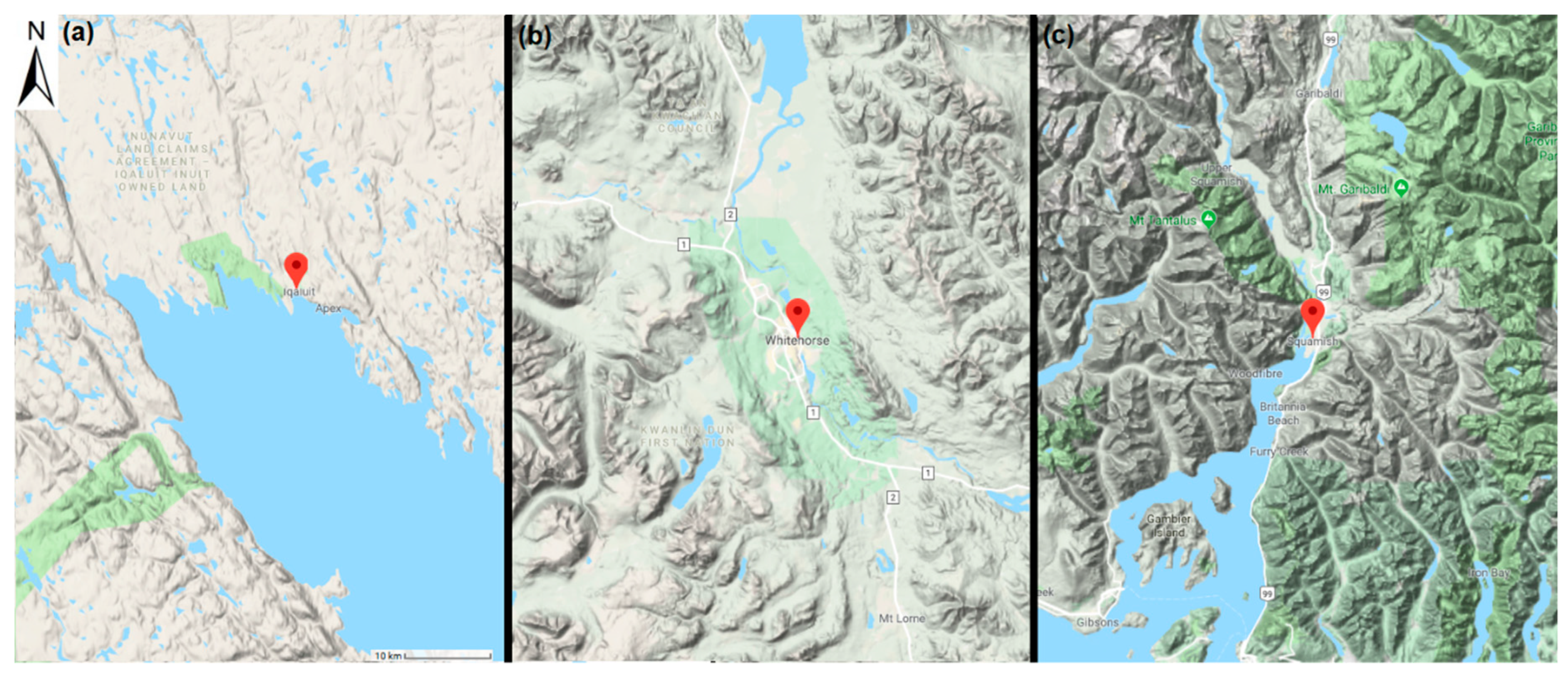
The Iqaluit supersite is situated in the Arctic tundra ~200 m from the shoreline of Frobisher Bay and ~200 m from the Iqaluit airport runway at 11 m Above Sea Level (ASL) (Figure 1a). The town is located in a valley that runs in the north-west to south-east direction. As such, the primary surface wind directions are from the NW and SE. The terrain is relatively flat with the exception of ~300 m-high hills located several kilometers north-east of the supersite. The site is equipped with a suite of remote-sensing instrumentation, including a Doppler Ka-band radar, a Doppler lidar, Raman and Differential Absorption Lidar (DIAL) water vapour lidars, a CL51 ceilometer, as well as a radiation flux sensor suite, a Far-infrared radiometer, several disdrometers and precipitation weighing gauges, radiosondes, and WMO-standard surface meteorological instruments [20,25]. The Doppler lidar is located ~40 m from where the radiosondes are launched and started collecting data in October 2015.
The Whitehorse supersite and Squamish site are located directly on airport property, <100 m from the airport runway (Figure 1b,c). Both sites are situated in complex mountainous terrain. Whitehorse (706 m ASL) is located in a valley that runs in the north-north-west direction between two mountains to its West (~1.6 km ASL) and East (~1.4 km ASL). Squamish (59 m ASL) is located in a narrow valley that runs north-north-east with mountains >2 km ASL to either side. The primary surface wind direction for both sites is along the valley. The sites are equipped with similar instrumentation as Iqaluit, including the same make and model of scanning Halo Doppler lidars, which started collecting data in November 2017 (Whitehorse) and May 2016 (Squamish).
2.2. Doppler Light Detection and Ranging (Lidar)
Similar to RWPs, the primary application for Doppler lidars is as a boundary layer wind profiler. Doppler lidars provide precise and accurate backscatter and Doppler velocity measurements at high temporal- and spatial-resolution along the lidar beam’s path (radial direction). As such, they have demonstrated the ability to measure fast-evolving meteorological features, such as lake breezes and low-level jets, and cloud microphysical properties [7,26,27,28,29].
Identical Halo Photonics Streamline XR scanning Doppler lidars were operated at all three sites using the same configuration settings and scan strategies. The lidars were fully autonomous and operated continuously, even during precipitation and severe weather events, with no operator intervention required. For instance, the Iqaluit lidar’s uptime was 92% (2016 to 2018), with almost all downtime caused by power outages at the site. The lidar observations are well-suited to complement existing radiosonde observations, particularly when extreme surface winds prevent radiosondes from being launched. In Iqaluit, this occurred 13% of the time (2015–2018 statistics), resulting in significant gaps in upper air observations [20] whereby the Doppler lidar was the sole source of upper air wind observations at the site during these times.
The Halo lidars operate at 1.5 µm using an 80 µJ pulsed laser at 10 kHz with a range resolution of 3 m (60 m range gates). The lidars are eye-safe, are fully customizable, and have full-scanning capability, allowing them to conduct measurements at any elevation and azimuth. The lidar cannot take measurements within the first range gate, resulting in a ‘blind spot’ within the first 60 m. All Doppler lidars were subjected to identical quality-control procedures based on their signal-to-noise ratio (SNR) within each range gate and filtering outliers and returns from clouds and rain droplets; details are provided in Mariani et al. [7].
The maximum range of the lidar is limited by the lidar’s design (e.g., pulse power and receiver sensitivity) and the atmospheric conditions (number of backscatterers to produce a sufficiently high SNR). As such, the maximum vertical range typically followed the boundary layer height and varied from one to three km Above Ground Level (AGL) in Iqaluit and two to four km AGL in Whitehorse. The lidars operated with identical repeating eight-minute scan sequences, performing vertical stare, plan-position indicator (constant elevation), range-height indicator (constant azimuth), Doppler beam-swinging (DBS), and velocity-azimuth display (VAD) scans; the latter two were processed to provide vertical wind-profile observations and are the focus of this study.
2.3. Doppler Lidar Wind-Profile Measurement Methodology
Initially developed for use by Doppler weather radars, several different scan strategies can be utilized to obtain measurements of the two-dimensional wind profile above a Doppler lidar. Of these, the DBS [14] and VAD [30,31] methods are the most widely-used. During a DBS scan, the lidar beam is pointed in three directions: vertically (90° elevation), East (e.g., at 70° elevation), and North (e.g., at 70° elevation). A VAD scan is similar to a DBS scan except that many azimuth angles are used so the lidar beam traces a cone at a single elevation angle. These additional azimuth angles help reduce the uncertainty in the retrieved two-dimensional wind components u and v. For a DBS wind profile, the uncertainty in u and v is estimated to be 0.32 m/s; for an 8-beam VAD profile it is <0.22 m/s [18].
In recent years, DBS and VAD wind-profile observations have been adopted into national and international standards and guidelines. DBS is much faster than a VAD scan [15]. For instance, the Halo lidars complete a DBS scan in 20 s versus a 90 s VAD scan using the same number of pulse averages. This makes DBS scans more suitable in urban environments, where the flow changes quickly in space and time. As such, DBS scans are more suitable than VAD scans only where the flow cannot be considered uniform over the volume sampled or steady over the time it takes to complete the VAD scan [14].
During this study, the DBS and VAD scans utilized a 70° elevation angle and eight VAD beams were used (spaced evenly apart, every 45° in azimuth). Horizontal homogeneity and zero convergence and deformation was assumed. From these scan geometries, the horizontal wind speed and direction can be retrieved above the lidar with a vertical resolution of approximately three metres as outlined in Lane et al. [15]. Note that each wind profile must be regarded as a snapshot of the wind profile at that particular time rather than a representation of the mean profile [15]. Both DBS and VAD scans were conducted in order to assess their performance with respect to Iqaluit radiosonde observations.
2.4. RS92 Radiosondes
Atmospheric profile observations from radiosondes are motivated largely by applications such as NWP and climate modeling and have a well-established history of providing reliable information [32]. Radiosondes provide high temporal and spatial resolution observations of the vertical wind profile (as well as other meteorological parameters) typically up to ~40 km AGL with high confidence.
Vaisala RS92 radiosondes [33] were launched twice a day (00 and 12 Coordinated Universal Time (UTC)) by the Meteorological Service of Canada as per WMO guidelines at the Iqaluit weather station (WMO station code 71909, CYFB). While the radiosonde valid time was 00 and 12 UTC, the actual launch occurred 40–45 min prior to this, i.e., ~23:15 UTC (day prior) and ~11:15 UTC. As such, all comparisons with the radiosonde were done based on its launch time.
The horizontal winds were retrieved based on the change of the sonde’s Global Positioning System (GPS) position. The radiosonde’s 2 s data sample rate provided a vertical resolution of roughly every 6 to 10 m (depending on the ascent speed). For RS92 radiosondes, the uncertainty estimates for the wind speed are 0.4 to 1 m/s and 1° for wind direction (Global Climate Observing System Reference Upper-Air Network, GRUAN, data processing) or 0.15 m/s in wind speed and 2° in wind direction (instrument manufacturer Vaisala) [32,33]; these uncertainties are based on 1σ statistical uncertainties.
Despite their advantages, radiosondes exhibit poor observation frequency (WMO standard is twice daily), cannot be launched during strong surface winds (>12 m/s), require substantial infrastructure and an operator at launch sites, and are subject to horizontal displacement in their observations. As such, the use of lidar wind profiling to complement radiosondes is currently under investigation. By comparing side-by-side lidar and radiosonde wind profiles at Iqaluit, the accuracy of the lidar’s wind-profile observations can be evaluated and the bias can be characterized using statistical methods.
3. Results and Discussion
3.1. Doppler Lidar and Radiosonde Comparisons
Nineteen months of coincident radiosonde and lidar observations at the Iqaluit supersite were compared (January 2016 to July 2017). Where necessary, radiosonde observations were interpolated to match the lidar observation altitudes. The closest lidar profile within 10 min after radiosonde launch was used to perform comparisons. A 10-min window was selected since this was about the time it took a radiosonde to reach 2 km AGL, which was near the Iqaluit lidar’s maximum vertical range. This helped ensure that the sonde was sampling air within vertical range of the lidar during each comparison. At ~2 km AGL, the radiosonde typically was ~6 km SE of the lidar, usually drifting over Frobisher Bay; this increasing horizontal displacement with height between the radiosonde and the lidar should be considered when interpreting their agreement.
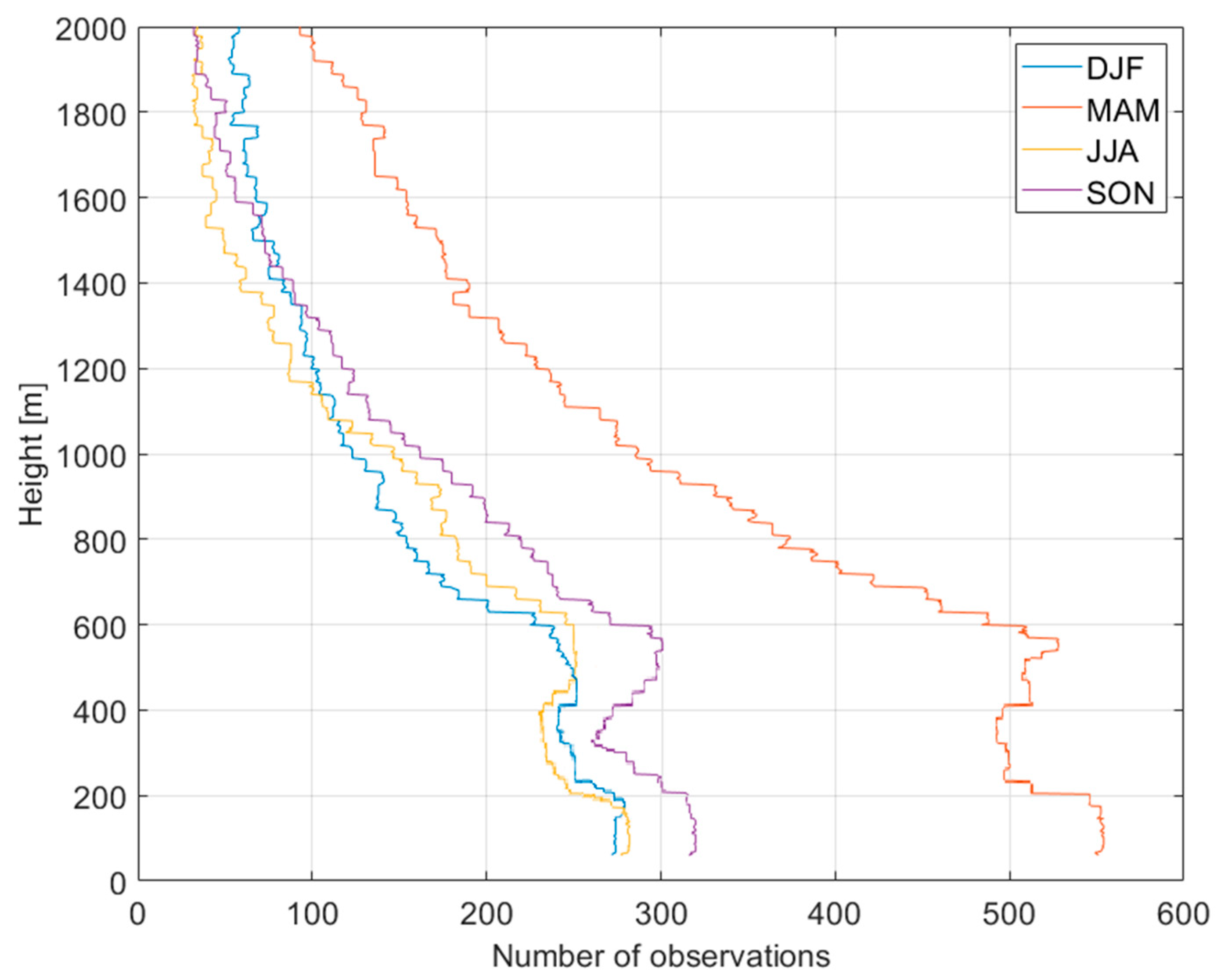
Figure 2 illustrates how the number of coincident observations decreased with height since the lidar obtained fewer observations at longer ranges. Other factors, including thick clouds and precipitation, attenuate the lidar’s signal and limit its ability to make measurements above the cloud base height, further limiting comparisons with the radiosonde at higher altitudes. The dip in the number of observations at around 300 m is likely due to topographical effects, including blowing snow from nearby hills, fog, and other meteorological effects that either reduced the lidar’s SNR or produced outliers at these heights that were filtered out as part of the lidar’s quality control processing. The observed difference between seasons is primarily due to the uneven study duration (most observation days and successful radiosonde launches happened to occur during March–May, MAM).
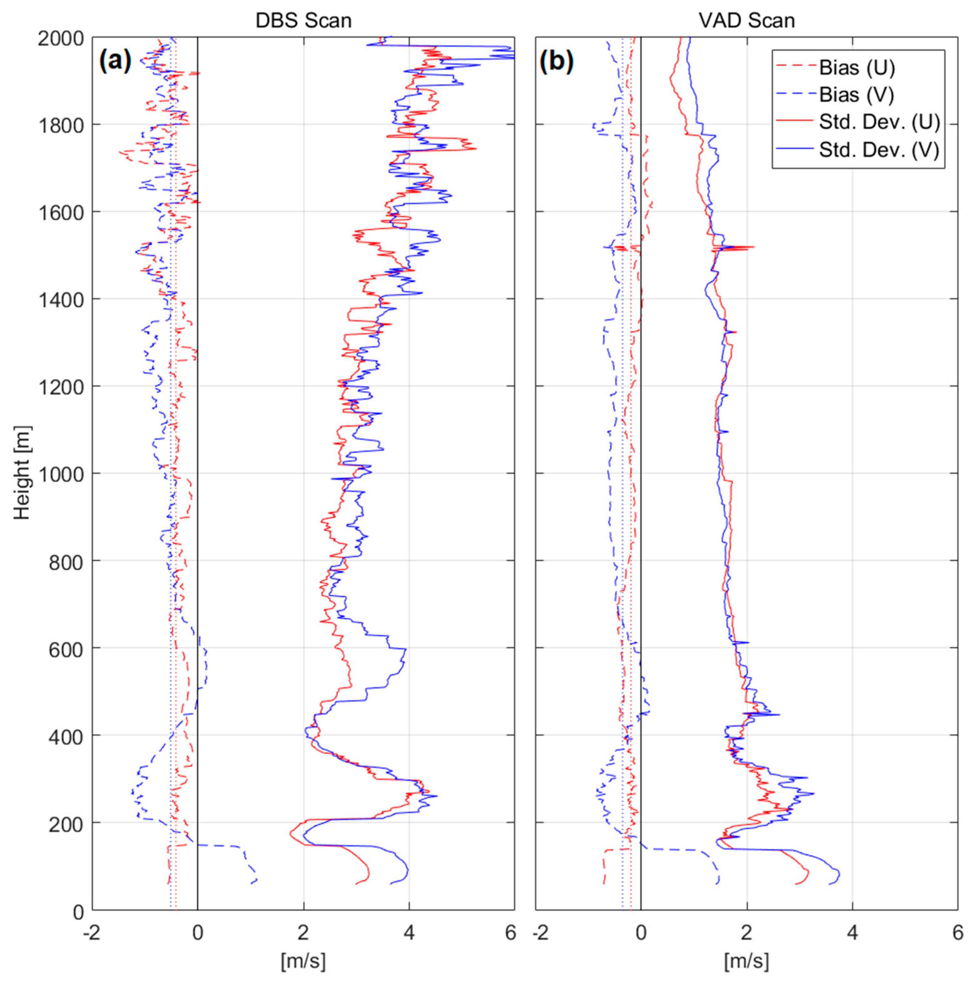
The bias and standard deviation of the error (STDE) between the lidar and radiosonde are provided in Figure 3 for both the DBS and VAD lidar scans. The bias was calculated as the mean difference between the lidar–radiosonde and the 1σ of the differences was used to characterize its uncertainty. Comparisons indicate good agreement for both the DBS and VAD scans, with an average bias of −0.46 ± 0.02 m/s (mean ± standard error of the mean, σ/√N) and R2 > 0.81 for DBS and −0.27 ± 0.02 m/s and R2 > 0.89 for VAD (for heights up to 2 km AGL). Overall the DBS scan exhibited a larger error and STDE than the VAD scan, which increased with height after approximately 1 km AGL. There was also significantly more structure and variability in the DBS’ STDE compared to the VAD. This is likely due to the fewer rays used to compute the DBS wind profile compared to the VAD. No seasonal dependence on the bias, R2, STDE, or root-mean-square error (RMSE) were found. Note that above 2 km AGL the STDE increased with height for both scan types due to radiosonde drift and the fewer number of comparisons available (and therefore it is not shown).
As an example of the lidar–sonde comparisons, the radiosonde wind profile on 2 February 2016 (11:18 UTC launch) is shown in Figure 4 (top panels) with three hours of lidar wind profiles (11:18 to 2:18 UTC) overlaid. Relatively good agreement (within ±3 m/s) during this time period was found due to low wind variability; the weaker winds on this day also caused minimal radiosonde horizontal displacement (Figure 4b). This was not typical for most radiosonde launches as the wind profile usually varied drastically on shorter timescales. The 24-hour plot of lidar VAD wind profiles observed on 7 February 2019 (Figure 4d) demonstrates the more typical wind variability at Iqaluit. Figure 4d also illustrates the lidar’s ability to fill the temporal gap in wind-profile observations at WMO radiosonde observation sites.
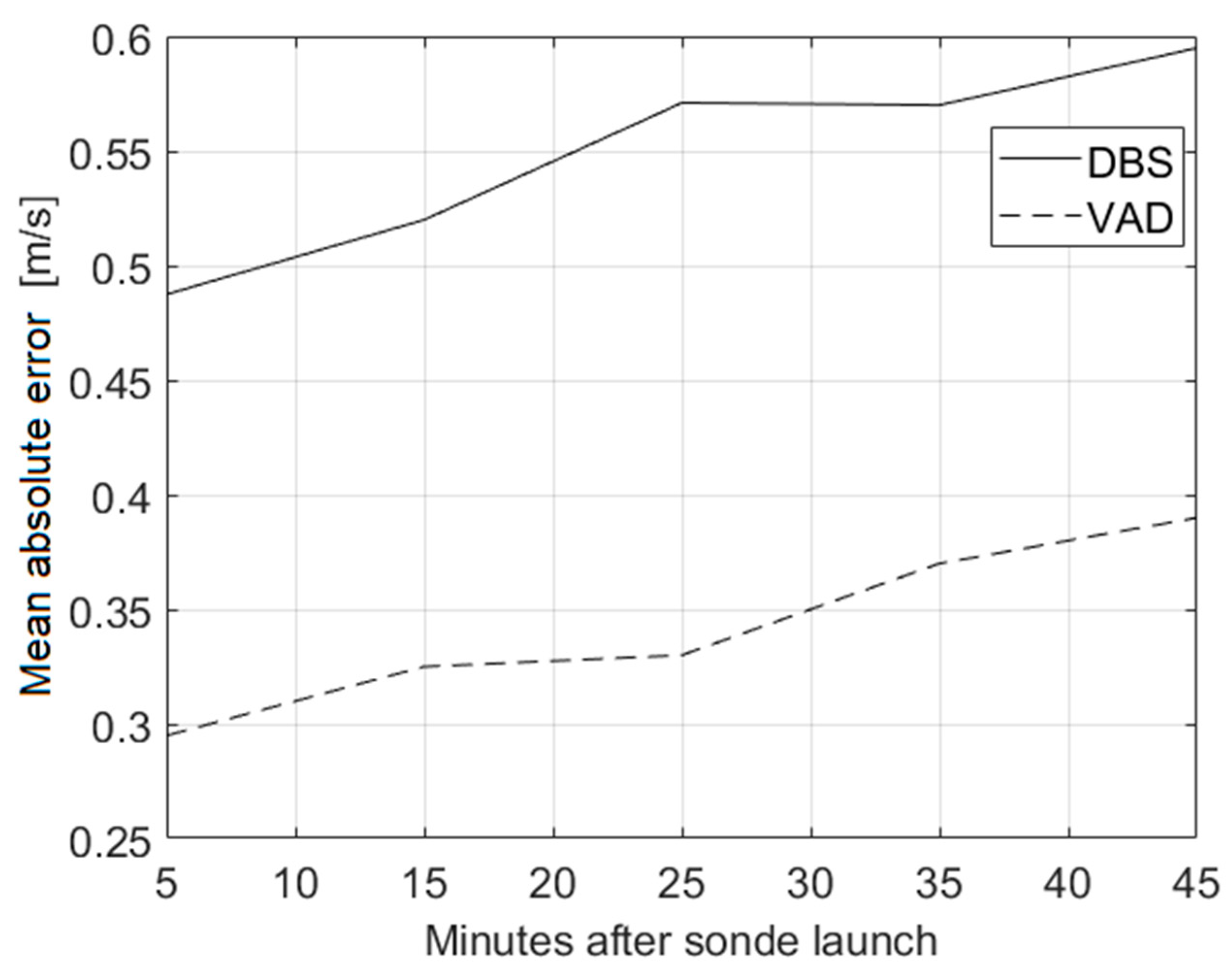
The lidar-sonde mean absolute error (averaged from 0 to 2 km AGL) increased when comparisons were performed at longer comparison times after the radiosonde launch time, as shown in Figure 5. This provides an indication of the temporal representativeness of the lidar wind-profile measurements, whereby on average the lidar-sonde absolute error increased roughly 0.13 m/s per hour after radiosonde launch regardless of scan type. From Figure 5 it is clear that comparisons within 0–10 min after radiosonde launch, which were used to produce Figure 3, exhibited the best agreement, when the sonde remained relatively close to the ground.
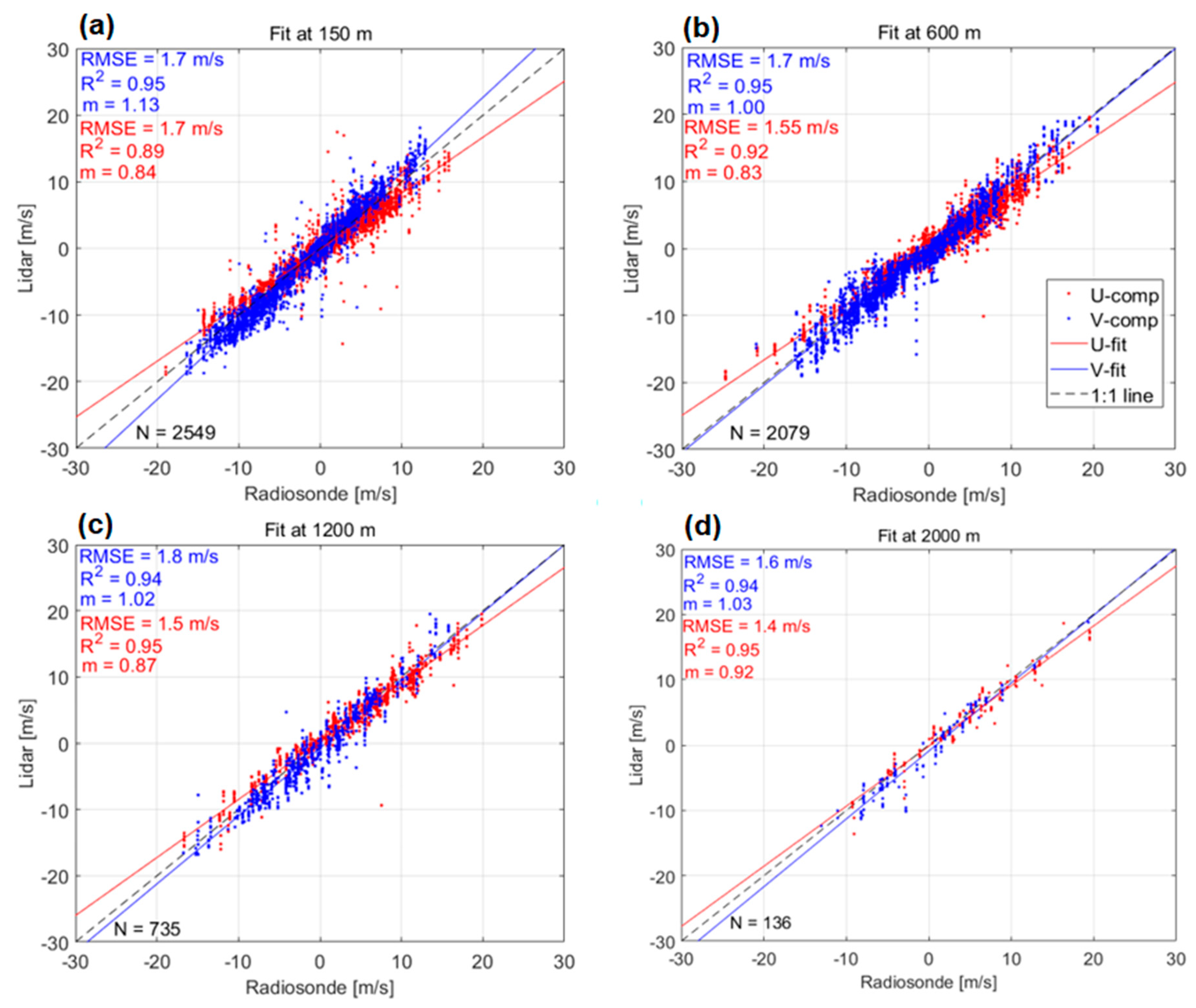
Coincident lidar and radiosonde observations were strongly correlated, as shown in Figure 6. This indicates excellent agreement between the two instruments at all heights within range of the lidar and is similar to the agreements found in previous studies [13,15,16,18,19]. Lidar DBS wind-profile correlations (not shown) exhibited slightly weaker correlations (e.g., R2 = 0.90, m = 1.05, and RMSE = 2.1 m/s at 150 m AGL) compared to the VAD correlations. No seasonal dependence was found.
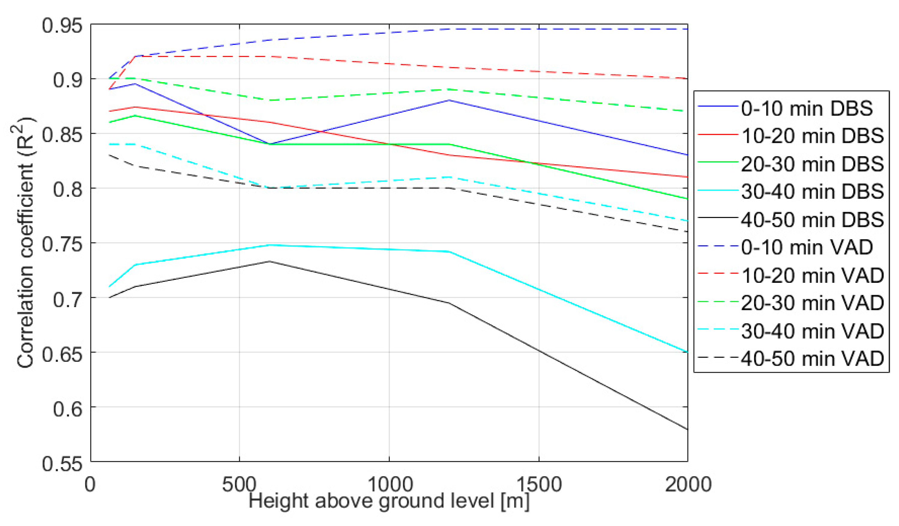
The correlations shown in Figure 6 depend on the altitude. As shown in Figure 7, the correlation (R2) for comparisons within 10 min of radiosonde launch decreased with height only for DBS wind profiles. This is in agreement with the DBS’ increase in the STDE with height (Figure 3) and similar to the lidar-radiosonde correlations provided in Kumer et al. [16]. The correlation strength decreased roughly 0.22 and 0.08 per hour after radiosonde launch for DBS and VAD scans, respectively. At longer comparison times (e.g., 40–50 min after radiosonde launch), both DBS and VAD R2 values decreased with height, but more so for DBS.
3.2. Verification of Numerical Weather Prediction (NWP) Models against the Doppler Lidar
3.2.1. Environment and Climate Change Canada (ECCC) NWP Models
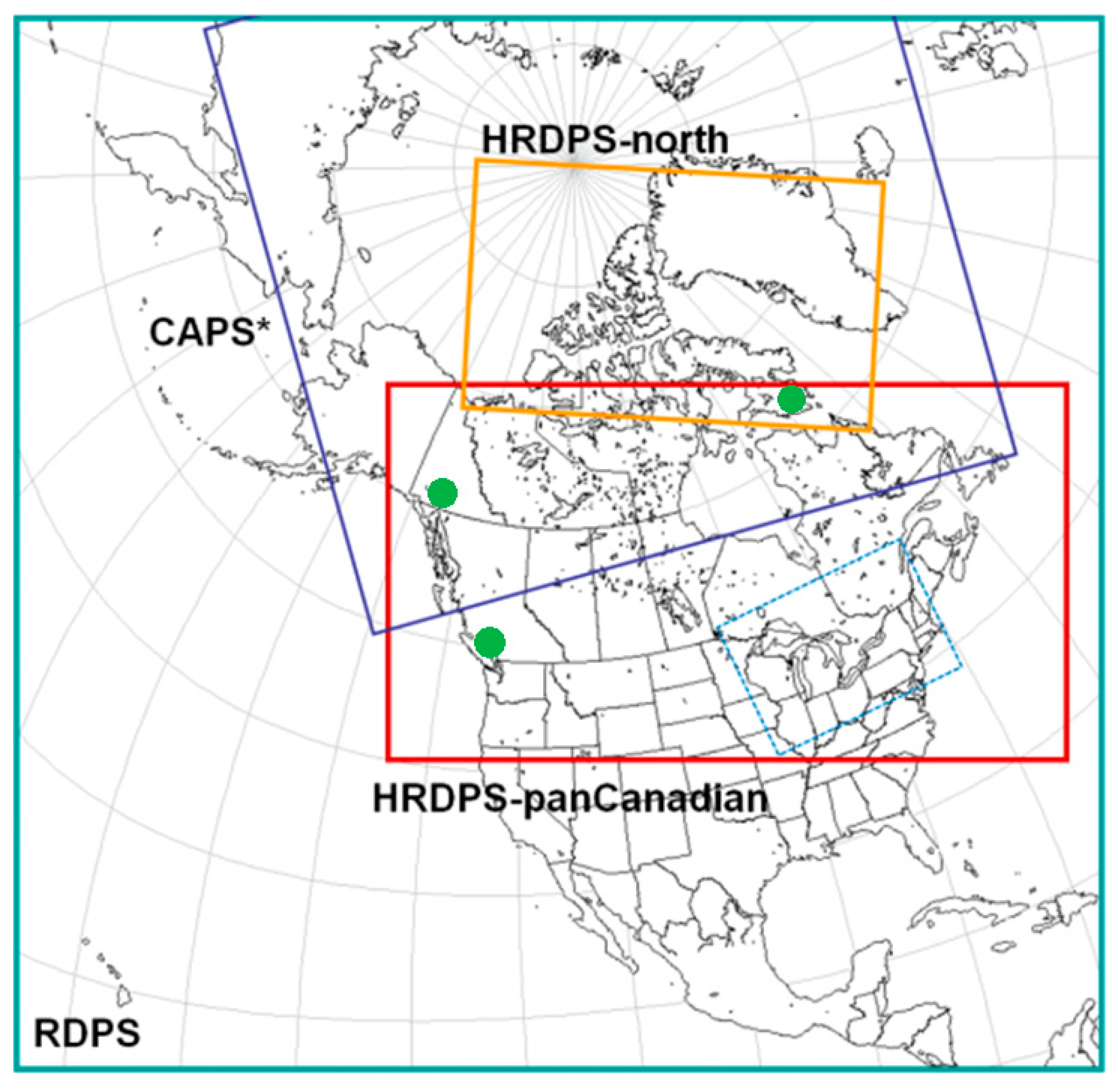
From 2016–2018, ECCC has run its deterministic prediction systems operationally with domains that cover most or all of the Arctic region (Figure 8). All of these models are based on the Canadian global environmental multiscale (GEM) model [34,35] and details on their initialization and surface scheme can be found in Bélair et al. [36] and Buehner et al. [37]. The regional deterministic prediction system (RDPS, ~10 km grid spacing) is a limited area model (LAM) nested within the global deterministic prediction system (GDPS, ~15 km grid spacing), which is fully coupled with the global ice and ocean prediction system (GIOPS) [38]. The high-resolution deterministic prediction system (HRDPS, ~2.5 km grid spacing) is in turn a LAM nested within the RDPS and resolved as in a scale-cascade. The Canadian Arctic prediction system (CAPS, ~3 km grid spacing) is nested within the GDPS and is an experimental model developed as ECCC’s contribution to the YOPP modeling effort. CAPS has been running operationally since February 2018 and is coupled with the regional ice and ocean prediction system (RIOPS) [39,40]. It has an enhanced microphysics scheme [41,42] and a large domain, encompassing the whole Arctic.
In alignment with the YOPP data access, CAPS gridded model output is available for research studies at http://dd.alpha.meteo.gc.ca/yopp/model_caps and CAPS high-frequency time series in a 7 × 7 grid surrounding the YOPP supersites (which include Iqaluit and Whitehorse) are available at http://thredds.met.no/thredds/catalog/alertness/YOPP_supersite/ECCC-CAPS/catalog.html. Radiosonde data are assimilated into the models every 12 h, unlike Doppler lidar data. Forecasts analyzed in this study are produced from model runs at 00 and 12 UTC and are valid for 48 h, since these are when the origin and lead times are common to all NWP models considered.
3.2.2. Model Verification
Comparisons between the RDPS, HRDPS (“HRDPS-panCanadian” in Figure 8), and CAPS model output and the Doppler lidar wind-profile observations were performed in this study. The Doppler lidar’s wind-profile observations were averaged in larger 30 m altitude bins to better match the model output’s lower vertical resolution. The models use sigma-hybrid vertical levels, therefore the models’ vertical structure is not uniform; vertical resolution is higher near the surface and jet stream. The models’ horizontal winds were linearly interpolated to 90, 150, and 300 m AGL, and then every 300 m above that up until 3.6 km AGL in order to perform comparisons with the lidar.
Lidar VAD wind profiles were compared to the 3-h lead-time forecast winds from RDPS, HRDPS, and CAPS. The mean bias (model output–lidar) and RMSE for Iqaluit, Whitehorse, and Squamish are provided in Figure 9; vertically averaged statistics are in Table 1. Output from each model’s grid point closest to the lidar was compared against all available lidar observations from January 2016 to September 2018 at each site. The number of comparisons ranged from N = 9 at higher altitudes (3.6 km AGL at Iqaluit) to N = 759 at lower altitudes (90 m AGL at Squamish). Similar results were obtained for the DBS wind profiles and for comparisons against 27- and 39-hour lead-time forecast winds, with the exception that the biases and RSME were slightly larger (not shown).
Good agreement comparable to the lidar–radiosonde was found at Iqaluit for all models (except for a large CAPS bias at altitudes above 2 km). The model versus lidar agreement at Whitehorse and Squamish was less strong than at Iqaluit, possibly due to the difficulty in the model’s ability to resolve the wind field in such complex mountainous terrain. In addition, no radiosonde measurements could be assimilated in the NWP initial conditions at Squamish due to none being available. The small constant positive bias at Iqaluit for altitudes above 500 m AGL is possibly due to the lidar’s systematic underestimation of wind speed (Figure 3). The bias at the Whitehorse site increased linearly with height between 500 m and 2 km AGL; the larger RDPS RMSE was mainly due to its larger bias. The model wind speeds at Squamish were underestimated at lower elevations (<1200 m AGL) and overestimated at higher elevations (>1200 m AGL), again with a better performance of the high-resolution model. As such, the low mean biases reported in Table 1 for Squamish are due to the large positive and negative biases averaging out; the RMSE is a more reliable metric in this case.
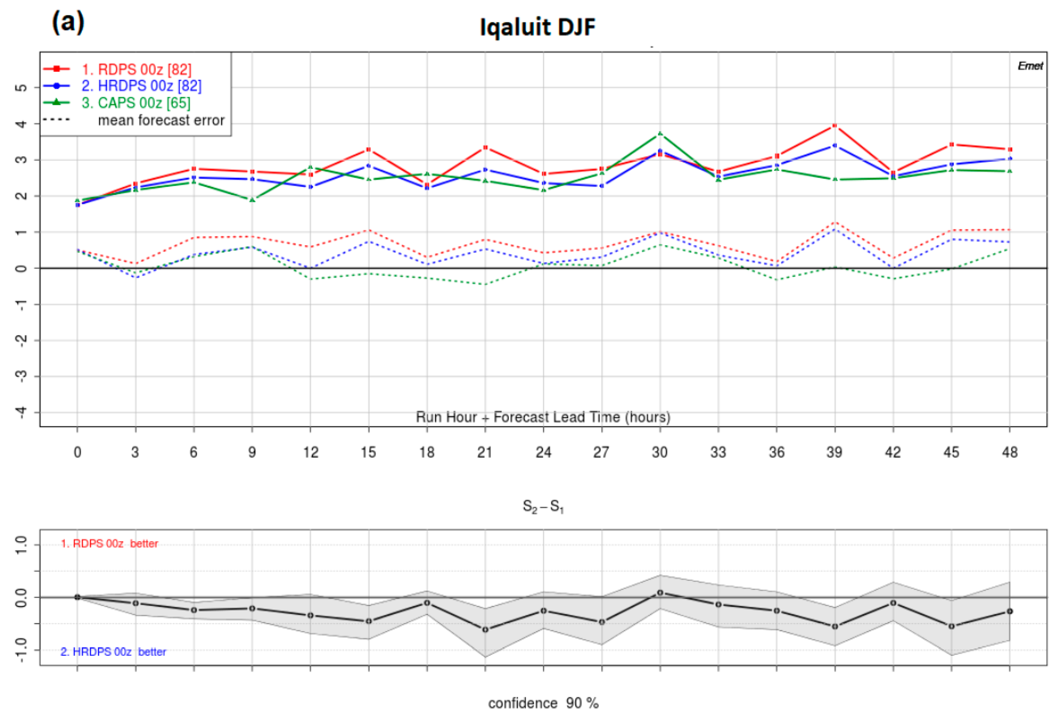
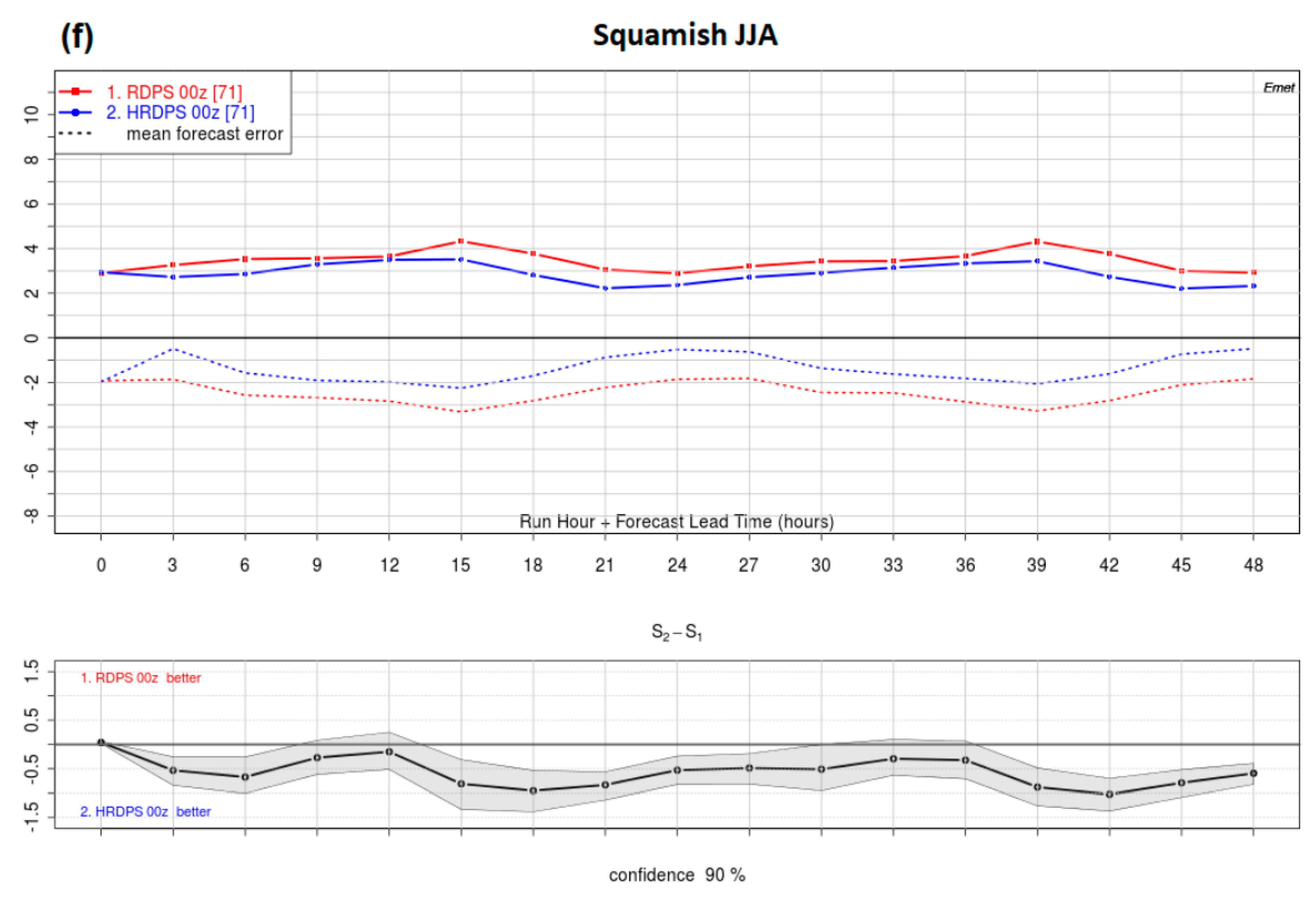
Results in Figure 10 are separated by season (winter = December to February 2017–2018, summer = June to August 2018) to illustrate the observed seasonal differences in the model-lidar agreement as a function of forecast lead time. This provides an initial evaluation of the GEM models’ wind fields during WMO’s 2018 YOPP period. Results shown are for comparisons at 900 m AGL but are representative of the agreement at most heights. Good agreement between the lidar and GEM models was found, particularly for the higher-resolution HRDPS and CAPS models and for Iqaluit (only during the winter at Squamish did RDPS outperform HRDPS). No significant increase in the bias or RMSE was observed as a function of forecast hour; the daily oscillation in biases and RMSE is typically a stronger signal than the forecast error increase with lead time within this forecast range. Overall, the agreement during the summer was better than that during the winter for all models. There was also significantly more variability in the bias and RMSE during the winter than the summer at all sites, indicating clear seasonal differences not only in the models’ performance but also in the verification sample size (fewer comparisons were available during the winter months).
4. Discussion
In this study, Halo Doppler lidar wind-profile observations were compared to coincident radiosonde observations at ECCC’s Iqaluit supersite over a 19-month period. Overall, excellent agreement was observed between the lidar–sonde. The larger bias and STDE within the first 150 m AGL for both scans (Figure 3) is likely the result of how radiosondes are launched; a tether that is released from the radiosonde at launch produces a torque, which causes the radiosonde to rotate below the balloon until it is stabilized. As such, wind speed measurements from the radiosonde in this lower region may be less reliable. For instance, Kumer et al. [16] found that the agreement between the lidar and sonde was better for heights > 125 m AGL.
A systematic negative bias between the lidar-sonde existed during all seasons and times of day, indicating that overall the lidar measures smaller wind speeds than the radiosonde. Note that the bias magnitude is comparable to the radiosonde wind speed uncertainty (0.4–1 m/s) as estimated by GRUAN, but is larger than the Vaisala estimates (0.15 m/s). The lidar-sonde agreements and correlations were similar to the agreements found in previous studies [13,15,16,18,19]. Comparing the two scan methodologies, the DBS scan exhibited an increase in the error with height, after approximately 1 km, whereas the VAD wind profiles’ agreement with the radiosonde remained relatively unchanged with height, despite the radiosonde’s drift. This could be due to the larger scanning volume during a VAD scan, whereas the DBS scan did not sample air to its south where the radiosonde typically drifted. Since the VAD scan agreed with the radiosonde better than the DBS scan in almost every regard and the requirement for an accurate VAD scan is uniform flow, the flow over the Iqaluit supersite and surrounding region, including the airport runway, can be considered uniform.
Comparisons between the lidar wind profiles and the ECCC operational GEM modeled winds showed good agreement that was better at Iqaluit (tundra) than at Whitehorse and Squamish (mountainous terrain). While this indicates difficulties with the models’ ability to resolve the wind field in mountainous terrain, note that these results are based on only three locations and may not be representative everywhere. The models also performed better during the summer than the winter; this is possibly due to the larger volume of data available during the summer in the Polar Regions, which improves the NWP initial conditions via data assimilation. A better understanding of summer polar processes might also play a role, however we believe the assimilation has a larger impact given that the model performance is almost constant with lead time.
5. Conclusions
Environment and Climate Change Canada (ECCC) has equipped several of its meteorological observation sites with Doppler lidars to investigate their ability to complement existing radiosonde observations and provide enhanced meteorological data for model verification and process studies during the World Meteorological Organization’s Year of Polar Prediction (YOPP). The Halo Doppler lidar Doppler beam swinging (DBS) and velocity-azimuth display (VAD) wind-profile observations were quality-controlled and compared against coincident radiosonde observations at ECCC’s Iqaluit supersite. The best agreements were found for comparisons within 10 min of radiosonde launch, which is when the radiosonde was still sampling air within range of the lidar.
Excellent agreement between the lidar and radiosonde was found during 19 months (January 2016 to July 2017) of continuous lidar observations. The mean bias between the lidar and radiosonde was −0.46 ± 0.02 m/s and −0.27 ± 0.02 m/s for DBS and VAD scans, respectively, which falls within the quoted uncertainty by both manufacturers. This small but systematic negative bias indicates that the lidar measures slightly lower wind speeds compared to the radiosonde regardless of season, scan strategy, or meteorological conditions. The lidar and radiosonde wind-profile measurements were also strongly correlated (R2 > 0.81 for DBS and R2 > 0.89 for the VAD, for heights up to 2 km AGL). The VAD scan agreed with the radiosonde better than the DBS scan in almost every regard. This evaluation of the lidar wind profiles provides a characterization of its error statistics in the Arctic as required for NWP model evaluation and assimilation, which is the focus of future work.
Doppler lidar wind-profile observations were compared to ECCC’s Numerical Weather Prediction (NWP) model output and showed good agreement with mean biases slightly larger than the lidar-sonde comparisons (e.g., 0.49 ± 0.08 m/s for HRDPS at Iqaluit). The models assimilated Iqaluit and Whitehorse radiosonde data, which exhibited slightly larger wind-speeds than the lidar: consequently, at Iqaluit and Whitehorse all models exhibited a small and systematic positive bias compared to the lidar. As expected for very local variables (such as near-surface winds), the higher-resolution models (Canadian Arctic prediction system, CAPS, and high-resolution deterministic prediction system, HRDPS) performed better than the coarser resolution regional deterministic prediction system (RDPS), exhibiting a smaller bias and root-mean-square error (RMSE).
The surrounding topography at the three sites had an impact on the model-lidar agreement. Overall the model-lidar agreements were worse in mountainous terrain, indicating difficulties with the models’ ability to resolve the wind field in mountainous terrain. At Iqaluit, the bias and RMSE peaked at the height of the nearby hills, as it did for the lidar-radiosonde comparisons. A negative bias was found near the surface for all models at Whitehorse and Squamish, whereas above the nearby mountains a large positive bias was found. This indicates that the model underestimates winds within the valley and overestimates winds above the mountains in mountainous terrain. However, only three locations were used in this evaluation and as such these results may not be representative of the models’ performance everywhere. All models performed better during the summer than the winter (except for RDPS at Squamish), whereas no differences between seasons were observed for the lidar–sonde comparisons. Further investigation is required to explain the change in model performance from winter to summer.
This study provides strong evidence for the lidar wind profiles to complement existing radiosonde wind observations, particularly when considering the ability of the lidar to provide autonomous (unmanned) additional observations within the boundary layer at significantly finer timescales and during all weather conditions. Changes in the winds that occur over timescales <12 h are currently not observed nor assimilated into ECCC NWP models; these gaps can be addressed by lidar wind-profile observations, albeit limited to the boundary layer, that exhibit similar accuracy to the radiosonde. A detailed assessment of the feasibility of assimilating lidar winds into the NWP model is currently underway at ECCC, and preliminary results indicate the additional information content provided from the lidar has a positive impact on NWP model performance over short to medium timescales (0–24 h forecasts).
Author Contributions
Conceptualization, Z.M.; methodology, Z.M., R.C., B.C., F.L.; formal analysis, Z.M., R.C., and B.C.; writing—original draft preparation, Z.M.; writing—review and editing, Z.M., R.C., B.C., F.L. All authors have read and agreed to the published version of the manuscript.
Funding
This research received no external funding.
Acknowledgments
Special thanks to Sorin Pinzariu, Michael Harwood, Robert Reed, Reno Sit, Jason Iwachow, and Daniel Coulombe for their help with instrumentation at the Iqaluit site. Thank you to the Meteorological Service of Canada radiosonde operators at Iqaluit for launching the radiosonde balloons. All data products are produced by ECCC and are available via obrs.ca or upon request.
Conflicts of Interest
The authors declare no conflict of interest.
References
- Courtney, M.; Wagner, R.; Lindelöw, P. Testing and comparison of lidars for profile and turbulence measurements in wind energy. In IOP Conference 170 Series: Earth and Environmental Science; IOP Publishing: Bristol, UK, 2008; Volume 1, p. 012021. Available online: http://0-stacks-iop-org.brum.beds.ac.uk/1755-1315/1/i=1/a=012021.0 (accessed on 1 October 2019).
- Pauscher, L.; Vasiljevic, N.; Callies, D.; Lea, G.; Mann, J.; Klaas, T.; Hieronimus, J.; Gottschall, J.; Schwesig, A.; Kühn, M.; et al. An inter-comparison study of multi-and DBS Lidar measurements in complex terrain. Remote Sens. 2016, 8, 782. [Google Scholar] [CrossRef] [Green Version]
- Banta, R.; Shepson, P.; Bottenheim, J.; Anlauf, K.; Wiebe, H.; Gallant, A.; Biesenthal, T.; Olivier, L.; Zhu, C.; McKendry, I.; et al. Nocturnal cleansing flows in a tributary valley. Atmos. Environ. 1997, 31, 2147–2162. [Google Scholar] [CrossRef]
- Banta, R.; Darby, L.S.; Kaufman, P.; Levinson, D.H.; Zhu, C.J. Wind flow patterns in the Grand Canyon as revealed by Doppler lidar. J. Appl. Meteorol. 1999, 38, 1069–1083. [Google Scholar] [CrossRef]
- Darby, L.S.; Neff, W.D.; Banta, R.M. Multiscale analysis of a meso-β frontal passage in the complex terrain of the Colorado Front Range. Mon. Weather Rev. 1999, 127, 2062–2081. [Google Scholar] [CrossRef]
- Fast, J.; Darby, L. An evaluation of mesoscale model predictions of down-valley and canyon flows and their consequences using Doppler lidar masurements during VTMX 2000. J. Appl. Meteorol. 2003, 43, 420–436. [Google Scholar] [CrossRef]
- Mariani, Z.; Dehghan, A.; Sills, D.M.; Joe, P. Observations of Lake Breeze Events during the Toronto 2015 Pan-American Games. Bound. Layer Meteorol. 2018, 166, 113–135. [Google Scholar] [CrossRef]
- Mariani, Z.; Dehghan, A.; Gascon, G.; Joe, P.; Hudak, D.; Strawbridge, K.; Corriveau, J. Multi-instrument observations of prolonged stratified wind layers at Iqaluit, Nunavut. Geophys. Res. Lett. 2018, 45, 1654–1660. [Google Scholar] [CrossRef] [Green Version]
- Illingworth, A.J.; Cimini, D.; Gaffard, C.; Haeffelin, M.; Lehmann, V.; Löhnert, U.; O’Connor, E.J.; Ruffieux, D. Exploiting existing ground-based remote sensing networks to improve high-resolution weather forecasts. Bull. Am. Meteorol. Soc. 2015, 96, 2107–2125. [Google Scholar] [CrossRef]
- Mizutani, K.; Itabe, T.; Yasui, M.; Aoki, T.; Murayama, Y.; Collins, R.L. Rayleigh lidar and Rayleigh Doppler lidar for measurement of the Arctic atmosphere. In Lidar Remote Sensing for Industry and Environment Monitoring; International Society for Optics and Photonics: Bellingham, WA, USA, 2001; Volume 4153. [Google Scholar] [CrossRef]
- Cohn, S.A.; Goodrich, R.K. Radar wind profiler radial velocity: A comparison with Doppler lidar. J. Appl. Meteorol. 2002, 41, 1277–1282. [Google Scholar] [CrossRef]
- Shaw, W.; Darby, L.; Banta, R. A comparison of winds measured by a 915 MHz wind profiling radar and a Doppler lidar, 83rd AMS annual meeting. In Proceedings of the 12th Symposium on Meteorological Observations and Instrumentation, Long Beach, CA, USA, 9–13 February 2003; Available online: https://ams.confex.com/ams/pdfpapers/58646.pdf (accessed on 1 October 2019).
- Ishii, S.; Mizutani, K.; Aoki, T.; Sasano, M.; Murayama, Y.; Itabe, T. Wind profiling with an eye-safe coherent Doppler lidar system: Comparison with radiosondes and VHF radar. J. Meteorol. Soc. Jpn. 2005, 83, 1041–1056. [Google Scholar] [CrossRef] [Green Version]
- Pearson, G.; Davies, F.; Collier, C. An analysis of the performance of the UFAM pulsed Doppler lidar for observing the boundary layer. J. Atmos. Ocean. Technol. 2009, 26, 240–250. [Google Scholar] [CrossRef]
- Lane, S.E.; Barlow, J.F.; Wood, C.R. An assessment of a three-beam Doppler lidar wind profiling method for use in urban areas. J. Wind Eng. Ind. Aerodyn. 2013, 119, 53–59. [Google Scholar] [CrossRef] [Green Version]
- Kumer, V.M.; Reuder, J.; Furevik, B.R. A comparison of LiDAR and radiosonde wind measurements. Energy Procedia 2014, 53, 214–220. [Google Scholar] [CrossRef] [Green Version]
- Achtert, P.; Brooks, I.M.; Brooks, B.J.; Moat, B.I.; Prytherch, J.; Persson, P.O.G.; Tjernström, M. Measurement of wind profiles by motion-stabilised ship-borne Doppler lidar. Atmos. Meas. Tech. 2015, 8, 4993–5007. [Google Scholar] [CrossRef] [Green Version]
- Paschke, E.; Leinweber, R.; Lehmann, V. An assessment of the performance of a 1.5 μm Doppler lidar for operational vertical wind profiling based on a 1-year trial. Atmos. Meas. Tech. 2015, 8, 2251–2266. [Google Scholar] [CrossRef] [Green Version]
- Newsom, R.K.; Brewer, W.A.; Wilczak, J.M.; Wolfe, D.E.; Oncley, S.P.; Lundquist, J.K. Validating precision estimates in horizontal wind measurements from a Doppler lidar. Atmos. Meas. Tech. 2017, 10, 1229–1240. [Google Scholar] [CrossRef] [Green Version]
- Joe, P.; Melo, S.; Burrows, W.; Casati, B.; Crawford, R.; Deghan, A.; Gascon, G.; Mariani, Z.; Milbrandt, J.; Strawbridge, K. The Canadian Arctic Weather Science Project: Introduction to the Iqaluit Site. Bull. Am. Meteorol. Soc. 2019. accepted. [Google Scholar] [CrossRef]
- Koltzow, M.; Casati, B.; Bazile, E.; Haiden, T.; Valkonen, T. An NWP model intercomparison of surface weather parameters in the European Arctic during the year of polar prediction special observing period northern hemisphere 1. Weather Forecast. 2019, 34, 959–983. [Google Scholar] [CrossRef]
- Riishojgaard, L. Wind Measurements in the WMO Global Observing System; ADM-Aeolus Science and Cal/Val Workshop; ESRIN: Frascati, Italy, 2015. [Google Scholar]
- Schyberg, H.; Randriamampianina, R. MET Norway Plans for Contribution to Calibration-Validation and Use of Aeolus Winds; ADM-Aeolus Science and Cal/Val Workshop; ESRIN: Frascati, Italy, 2015. [Google Scholar]
- Cassano, J.; Higgins, M.; Seefeldt, M. Performance of the Weather Research and Forecasting model for month-long pan-Arctic simulations. Mon. Weather Rev. 2011, 139, 3469–3488. [Google Scholar] [CrossRef]
- Mariani, Z.; Dehghan, A.; Gascon, G.; Joe, P.; Strawbridge, K.; Burrows, W.; Melo, S. Iqaluit calibration/validation supersite for meteorological satellites. In Proceedings of the Living Planet Symposium 2016 Conference, Prague, Czech Republic, 9–13 May 2016; Volume SP-740, p. 528, ISBN 978-92-9221-305-3. [Google Scholar]
- Dabas, A.; Drobinski, P.; Reitebuch, O.; Richard, E.; Delville, P.; Flamant, P.H.; Werner, C. Multi-scale analysis of a straight jet streak using numerical analyses and an airborne Doppler lidar. Geophys. Res. Lett. 2003, 30, 1049. [Google Scholar] [CrossRef]
- Baumgarten, G.; Fiedler, J.; Hildebrand, J.; Lubken, F.-J. Inertia gravity wave in the stratosphere and mesosphere observed by Doppler wind and temperature lidar. Geophys. Res. Lett. 2015, 42, 10929–10939. [Google Scholar] [CrossRef]
- Myagkov, A.; Seifert, P.; Bauer-Pfundstein, M.; Wandinger, U. Cloud radar with hybrid mode towards estimation of shape and orientation of ice crystals. Atmos. Meas. Tech. 2016, 9, 469–489. [Google Scholar] [CrossRef] [Green Version]
- Joe, P.; Bélair, S.; Bernier, N.B.; Brook, J.R.; Brunet, D.; Bouchet, V.; Burrows, W.; Charland, J.P.; Dehghan, A.; Driedger, N.; et al. The Pan-American games science showcase project. Bull. Am. Meteorol. Soc. 2017, 99, 921–953. [Google Scholar] [CrossRef]
- Lhermitte, R.M.; Atlas, D. Precipitation motion by pulse Doppler radar. In Proceedings of the Ninth Weather Radar Conference, Kansas City, MO, USA, 23–26 October 1961; American Meteorological Society: Boston, MA, USA, 1961; pp. 218–223. [Google Scholar]
- Browning, K.A.; Wexler, R. The determination of kinematic properties of a wind field using Doppler radar. J. App. Meteorol. 1968, 7, 105–113. [Google Scholar] [CrossRef]
- Dirksen, R.J.; Sommer, M.; Immler, F.J.; Hurst, D.F.; Kivi, R.; Vömel, H. Reference quality upper-air measurements: GRUAN data processing for the Vaisala RS92 radiosonde. Atmos. Meas. Tech. 2014, 7, 4463–4490. [Google Scholar] [CrossRef] [Green Version]
- Vaisala. Vaisala Radiosonde RS92 Measurement Accuracy; Technical Report; Vaisala: Vantaa, Finland, 2007. [Google Scholar]
- Côté, J.; Gravel, S.; Méthot, A.; Patoine, A.; Roch, M.; Staniforth, A. The operational CMC–MRB Global Environmental Multiscale (GEM) model: Part I. Design considerations and formulation. Mon. Weather Rev. 1998, 126, 1373–1395. [Google Scholar] [CrossRef]
- Girard, C.; Plante, A.; Desgagne, M.; McTaggart-Cowan, R.; Cote, J.; Charron, M.; Gravel, S.; Lee, V.; Patoine, A.; Qaddouri, A.; et al. Staggered Vertical Discretization of the Canadian Environmental Multiscale (GEM) model using a coordinate of the log-hydrostatic-pressure type. Mon. Weather Rev. 2014, 142, 1183–1196. [Google Scholar] [CrossRef]
- Bélair, S.; Crevier, L.-P.; Mailhot, J.; Bilodeau, B.; Delage, Y. Operational implementation of the ISBA land surface scheme in the Canadian regional weather forecast model. Part I: Warm season results. J. Hydrometeorol. 2003, 4, 352–370. [Google Scholar] [CrossRef]
- Buehner, M.; McTaggart-Cowan, R.; Beaulne, A.; Charette, C.; Garand, L.; Heilliette, S.; Lapalme, E.; Lapalme, E.; Macpherson, S.R.; Zadra, A.; et al. Implementation of deterministic weather forecasting systems based on ensemble–variational data assimilation at Environment Canada. Part I: The global system. Mon. Weather Rev. 2015, 143, 2532–2559. [Google Scholar] [CrossRef]
- Smith, G.C.; Roy, F.; Reszka, M.; Colan, D.S.; He, Z.; Deacu, D.; Belanger, J.-M.; Skachko, S.; Liu, Y.; Dupont, F.; et al. Sea ice forecast verification in the Canadian Global Ice Ocean Prediction System. Q. J. R. Meteorol. Soc. 2016, 142, 659–671. [Google Scholar] [CrossRef] [Green Version]
- Dupont, F.; Higginson, S.; Bourdallé-Badie, R.; Lu, Y.; Roy, F.; Smith, G.C.; Lemieux, J.-F.; Garric, G.; Davidson, F. A high-resolution ocean and sea-ice modelling system for the Arctic and North Atlantic oceans. Geosci. Model Dev. 2015, 8, 1577–1594. [Google Scholar] [CrossRef] [Green Version]
- Lemieux, J.-F.; Beaudoin, C.; Dupont, F.; Roy, F.; Smith, G.C.; Shlyaeva, A.; Buehner, M.; Caya, A.; Chen, J.; Carrieres, T.; et al. The Regional Ice Prediction System (RIPS): Verification of forecast sea ice concentration. Q. J. R. Meteorol. Soc. 2016, 142, 632–643. [Google Scholar] [CrossRef]
- Morrison, H.; Milbrandt, J. Parameterization of cloud microphysics based on the prediction of bulk ice particle properties. Part I: Scheme description and idealized tests. J. Atmos. Sci. 2015, 72, 287–311. [Google Scholar] [CrossRef]
- Milbrandt, J.; Morrison, H. Parameterization of cloud microphysics based on the prediction of bulk ice particle properties. Part III: Introduction of multiple free categories. J. Atmos. Sci. 2016, 73, 975–995. [Google Scholar] [CrossRef]
Figure 1.
Topographical map of the region around Iqaluit (a), Whitehorse (b), and Squamish (c). The hills to the East of Iqaluit (11 m ASL) have a height of ~300 m compared to the ~1.6 km and ~2 km ASL mountain ranges to the West of Whitehorse (706 m ASL) and Squamish (59 m ASL), respectively. Image © 2019 Google.

Figure 2.
Number of coincident light detection and ranging (lidar)-radiosonde observations for each season used in the comparison study (winter (DJF), spring (MAM), summer (JJA), and fall (SON)).
Figure 2.
Number of coincident light detection and ranging (lidar)-radiosonde observations for each season used in the comparison study (winter (DJF), spring (MAM), summer (JJA), and fall (SON)).

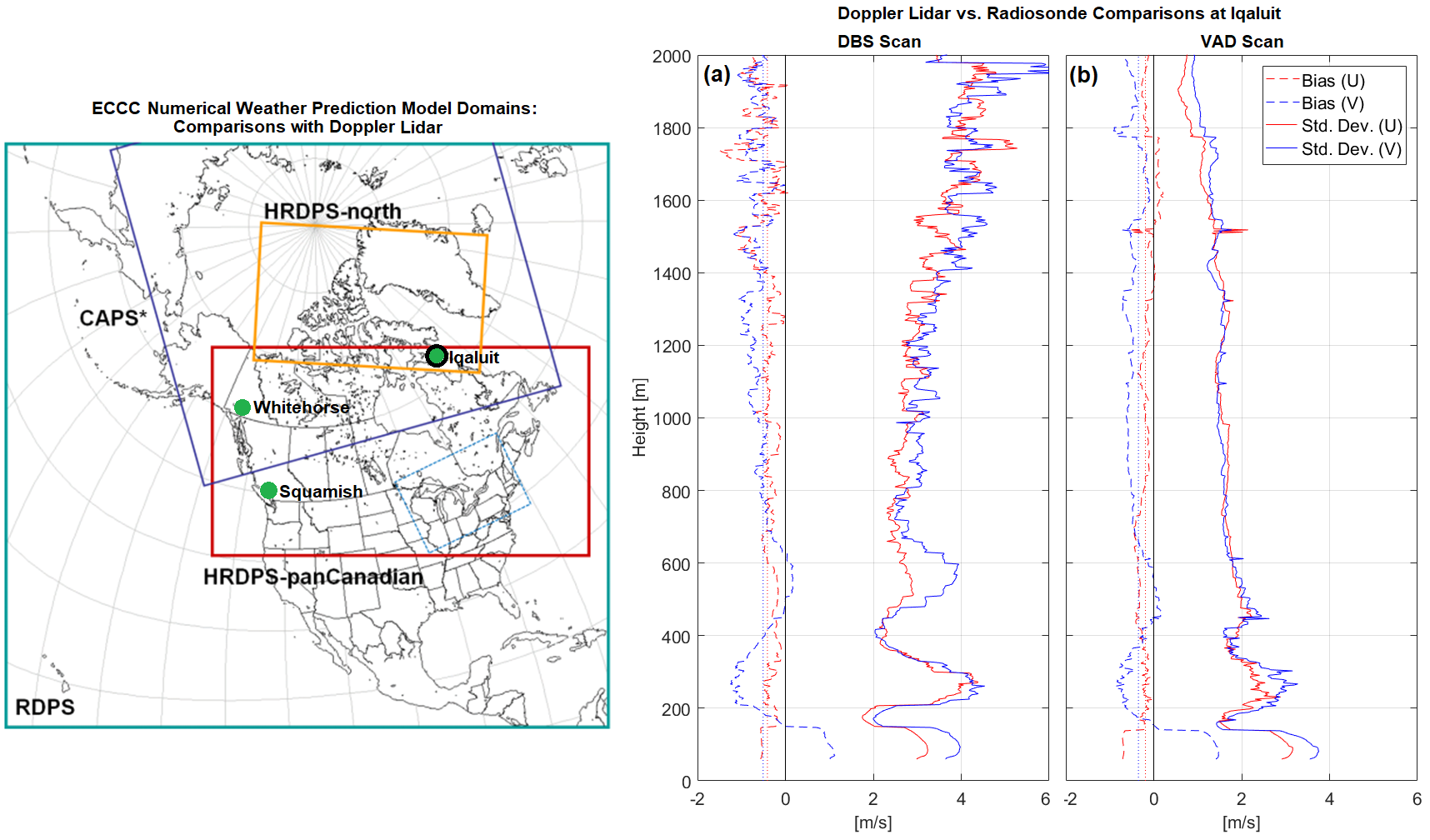
Figure 3.
Doppler beam-swinging (DBS) (a) and velocity-azimuth display (VAD) (b) lidar-sonde bias (mean difference, dashed line) and standard deviation of the error (STDE, solid line) for all coincident observations within 10 min of radiosonde launch. Both the u (red) and v (blue) components of the wind vector are shown. The mean biases from 0 to 2 km AGL are also shown (dotted vertical line).

Figure 4.
Radiosonde wind profile (green) at 11:18 UTC on 2 February 2016 overlaid with three hours (11:18-2:18 UTC) of lidar VAD wind profiles (black dashes) for the v (a) and u (c) wind components. Radiosonde drift distance compared to the lidar’s 70° beam divergence is also shown (b). 24 h of continuous lidar VAD wind-profile observations on 7 February 2019 are shown for comparison (d). Note: lidar wind profiles every 30 min and at every 99 m in height were plotted for clarity. Periods of radiosonde observations are indicated by the black rectangles.

Figure 5.
Mean absolute error (|lidar–sonde|) for different comparison times after sonde launch for the DBS (solid) and VAD (dashed) wind profiles. Comparison times were binned in 10-min increments.
Figure 5.
Mean absolute error (|lidar–sonde|) for different comparison times after sonde launch for the DBS (solid) and VAD (dashed) wind profiles. Comparison times were binned in 10-min increments.

Figure 6.
Correlations between lidar VAD and radiosonde wind profiles for all coincident observations within 10 min of radiosonde launch at altitudes 150 m (a), 600 m (b), 1200 m (c), and 2000 m (d) AGL. Linear fits for the u (red) and v (blue) components are shown along with the 1:1 line (black dash).

Figure 7.
Change in R2 as a function of height for the lidar DBS (solid) and VAD (dashed) wind profiles within 10 min of radiosonde launch (blue). Also shown are the R2 values for lidar comparisons 10 to 20 (red), 20 to 30 (green), 30 to 40 (teal), and 40 to 50 (black) min after radiosonde launch.
Figure 7.
Change in R2 as a function of height for the lidar DBS (solid) and VAD (dashed) wind profiles within 10 min of radiosonde launch (blue). Also shown are the R2 values for lidar comparisons 10 to 20 (red), 20 to 30 (green), 30 to 40 (teal), and 40 to 50 (black) min after radiosonde launch.

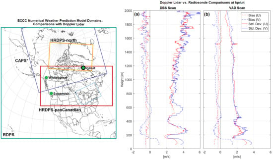
Figure 8.
Environment and Climate Change Canada (ECCC) deterministic prediction system domains for high-resolution deterministic prediction system (HRDPS, ~2.5 km grid spacing; red), Canadian Arctic prediction system (CAPS, ~3 km grid spacing; blue), and regional deterministic prediction system (RDPS, ~10 km grid spacing; cyan). HRDPS-north (orange) was not used in this study. Green circles indicate the locations of Iqaluit, Whitehorse, and Squamish (top to bottom).

Figure 9.
Three-hour forecast lead time model-lidar average bias (dashed) and root-mean-square error (RMSE, solid) for the RDPS (red), HRDPS (blue), and CAPS (green) model output above Iqaluit (a), Whitehorse (b), and Squamish (c) from Jan 2016 to Sept 2018. Black arrows indicate the approximate height of the top of the nearest mountain/hill relative to the lidar. The mean biases from 0 to 3.6 km AGL are also shown (dotted vertical line). Note: Squamish falls outside the CAPS domain.

Figure 10.
RDPS (red), HRDPS (blue), and CAPS (green) model bias (dashed) and RMSE (solid) compared to the lidar VAD wind profile as a function of forecast lead time for Iqaluit (a,b), Whitehorse (c,d), and Squamish (e,f). Results are shown for comparisons at 900 m AGL. Differences between the RDPS and HRDPS RMSE are shown in the panels underneath (grey shading indicates 90% confidence intervals). Comparisons during the winter are shown in the top two rows (a,c,e); summer is shown in the bottom two rows (b,d,f).


Table 1.
Three-hour lead time forecast mean bias (model-lidar, from 0 to 3.6 km AGL) and RMSE for RDPS, HRDPS, and CAPS at Iqaluit, Whitehorse, and Squamish. Note: Squamish falls outside the CAPS domain.
Table 1.
Three-hour lead time forecast mean bias (model-lidar, from 0 to 3.6 km AGL) and RMSE for RDPS, HRDPS, and CAPS at Iqaluit, Whitehorse, and Squamish. Note: Squamish falls outside the CAPS domain.
| Iqaluit Bias (m/s) | Iqaluit RMSE (m/s) | Whitehorse Bias (m/s) | Whitehorse RMSE (m/s) | Squamish Bias (m/s) | Squamish RMSE (m/s) | |
|---|---|---|---|---|---|---|
| RDPS 201601-201810 | 0.53 ± 0.08 | 2.69 | 1.79 ± 0.13 | 4.56 | 0.01 ± 0.16 | 3.69 |
| HRDPS 201601-201810 | 0.49 ± 0.08 | 2.64 | 1.49 ± 0.08 | 3.67 | 0.17 ± 0.05 | 2.76 |
| CAPS 201802-201810 | 0.71 ± 0.09 | 2.47 | 1.44 ± 0.08 | 3.71 | N/A | N/A |
© 2020 by the authors. Licensee MDPI, Basel, Switzerland. This article is an open access article distributed under the terms and conditions of the Creative Commons Attribution (CC BY) license (http://creativecommons.org/licenses/by/4.0/).
Share and Cite
MDPI and ACS Style
Mariani, Z.; Crawford, R.; Casati, B.; Lemay, F. A Multi-Year Evaluation of Doppler Lidar Wind-Profile Observations in the Arctic. Remote Sens. 2020, 12, 323. https://0-doi-org.brum.beds.ac.uk/10.3390/rs12020323
AMA Style
Mariani Z, Crawford R, Casati B, Lemay F. A Multi-Year Evaluation of Doppler Lidar Wind-Profile Observations in the Arctic. Remote Sensing. 2020; 12(2):323. https://0-doi-org.brum.beds.ac.uk/10.3390/rs12020323
Chicago/Turabian StyleMariani, Zen, Robert Crawford, Barbara Casati, and François Lemay. 2020. "A Multi-Year Evaluation of Doppler Lidar Wind-Profile Observations in the Arctic" Remote Sensing 12, no. 2: 323. https://0-doi-org.brum.beds.ac.uk/10.3390/rs12020323
Note that from the first issue of 2016, this journal uses article numbers instead of page numbers. See further details here.