Comparing Performances of Five Distinct Automatic Classifiers for Fin Whale Vocalizations in Beamformed Spectrograms of Coherent Hydrophone Array

Abstract

A large variety of sound sources in the ocean, including biological, geophysical, and man-made, can be simultaneously monitored over instantaneous continental-shelf scale regions via the passive ocean acoustic waveguide remote sensing (POAWRS) technique by employing a large-aperture densely-populated coherent hydrophone array system. Millions of acoustic signals received on the POAWRS system per day can make it challenging to identify individual sound sources. An automated classification system is necessary to enable sound sources to be recognized. Here, the objectives are to (i) gather a large training and test data set of fin whale vocalization and other acoustic signal detections; (ii) build multiple fin whale vocalization classifiers, including a logistic regression, support vector machine (SVM), decision tree, convolutional neural network (CNN), and long short-term memory (LSTM) network; (iii) evaluate and compare performance of these classifiers using multiple metrics including accuracy, precision, recall and F1-score; and (iv) integrate one of the classifiers into the existing POAWRS array and signal processing software. The findings presented here will (1) provide an automatic classifier for near real-time fin whale vocalization detection and recognition, useful in marine mammal monitoring applications; and (2) lay the foundation for building an automatic classifier applied for near real-time detection and recognition of a wide variety of biological, geophysical, and man-made sound sources typically detected by the POAWRS system in the ocean.

1. Introduction

A large-aperture densely-populated coherent hydrophone array system typically detects hundreds of thousands to millions of acoustic signals in the 10 Hz to 4000 Hz frequency range for each day of observation in a continental shelf ocean via the passive ocean acoustic waveguide remote sensing (POAWRS) technique [1,2]. The acoustic signal detections include both broadband transient and narrowband tonal signals from a wide range of natural and man-made sound sources [3,4,5,6,7], such as marine mammal vocalizations [1,2,8,9,10,11], fish grunts, ship radiated sound [12,13], and seismic airgun signals [14]. Here, we focus our efforts on developing automatic classifers for fin whale vocalizations detected in the Norwegian and Barents Seas during our Norwegian Sea 2014 Experiment (NorEx14) [1]. The fin whale vocalization signals have been previously detected, identified and manually labeled via semiautomatic analysis followed by visual inspection.

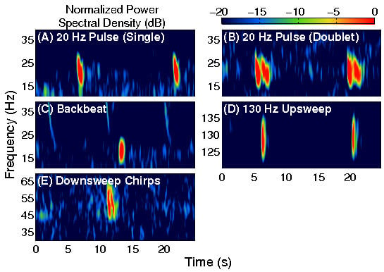
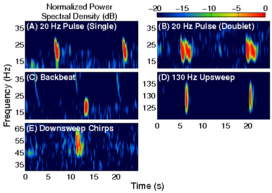
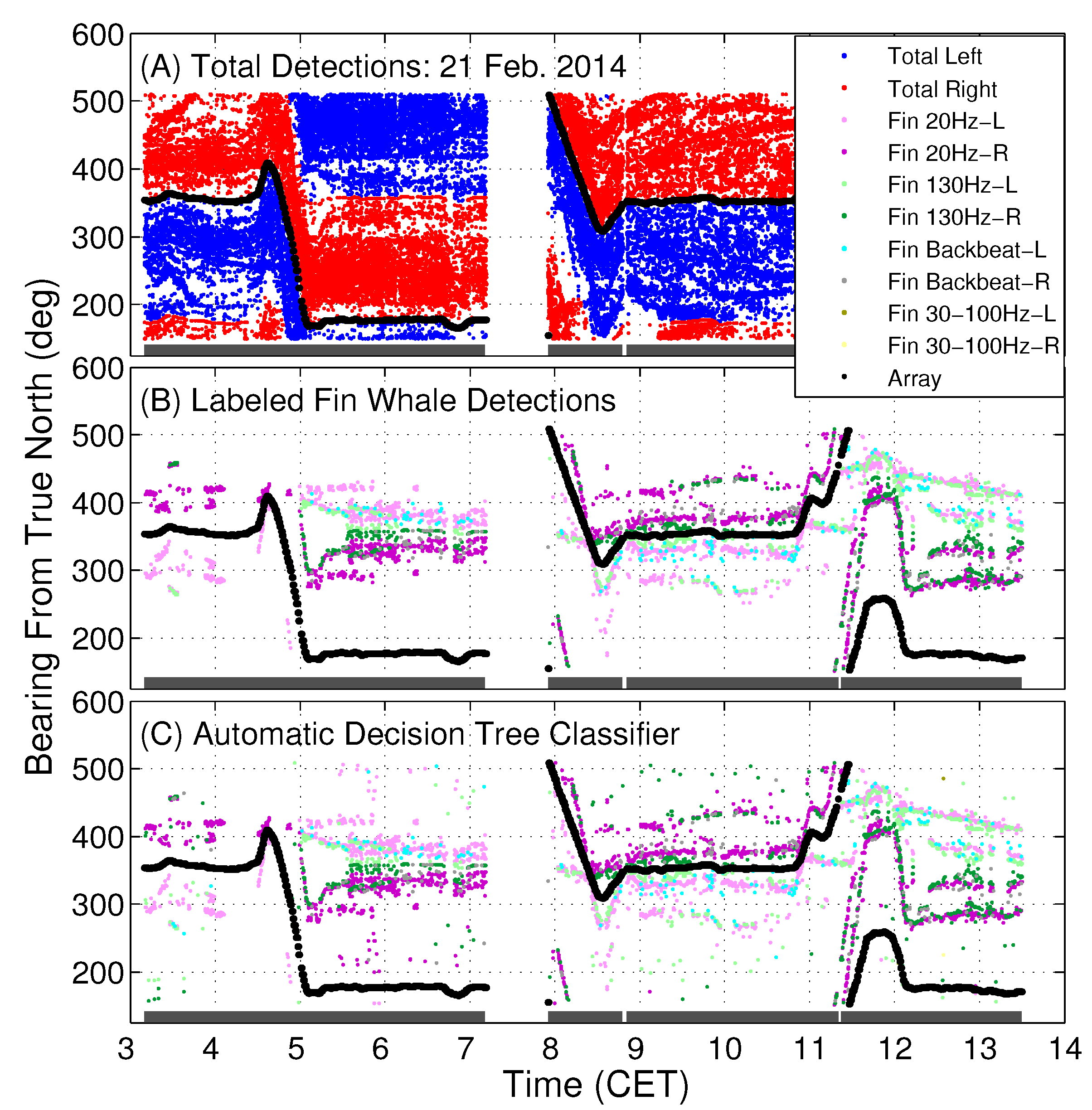
A total of approximately 170,000 fin whale vocalizations have been identified and extracted from the coherent hydrophone array recordings of NorEx14 [1]. The main types of fin whale vocalizations observed were the 20 Hz pulse, the 18–19 Hz backbeat pulse, the 130 Hz upsweep pulse, and the 30–100 Hz downsweep chirp [1,15,16,17,18]. Typical spectrograms for each of these fin whale vocalizations are displayed in Figure 1.

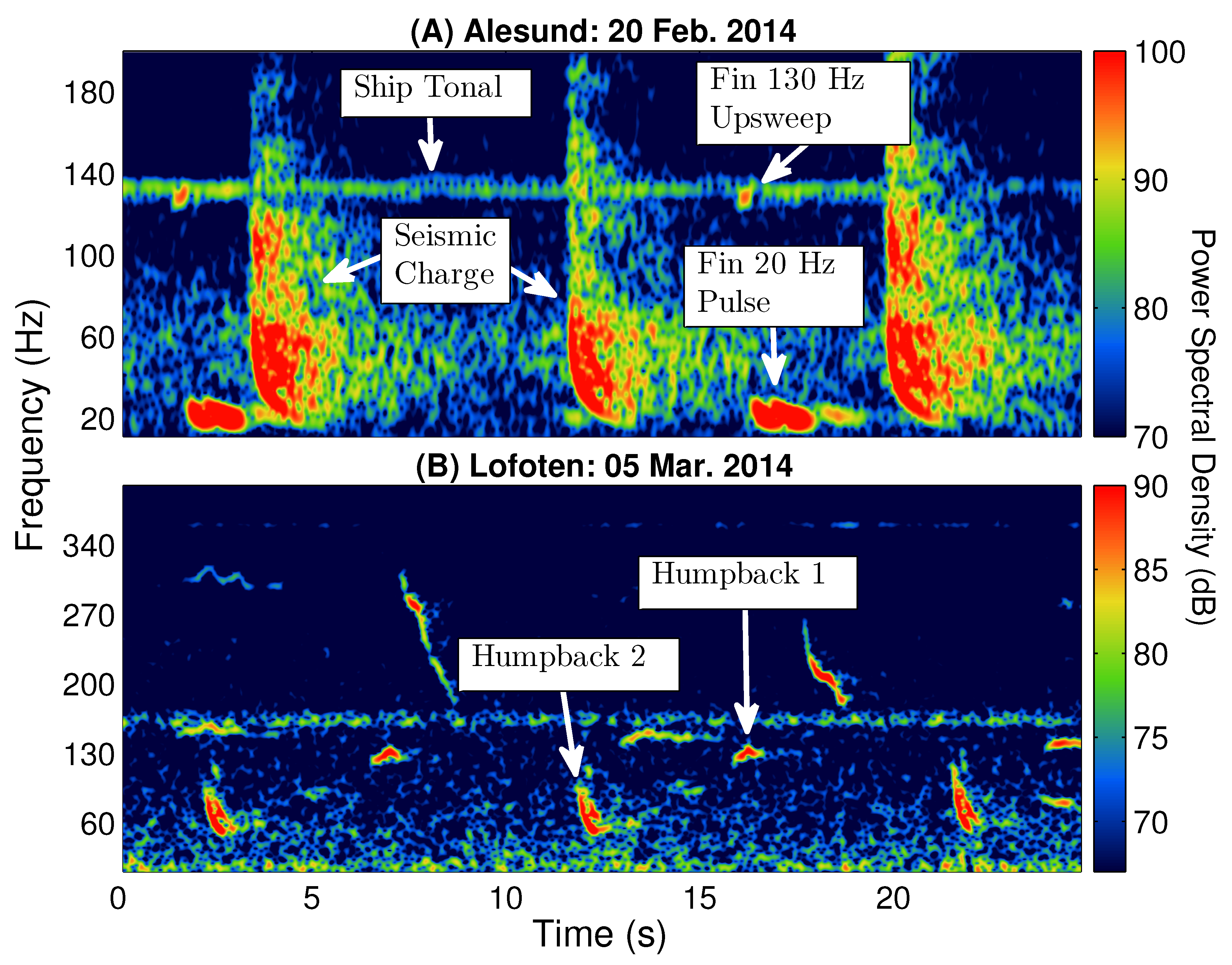
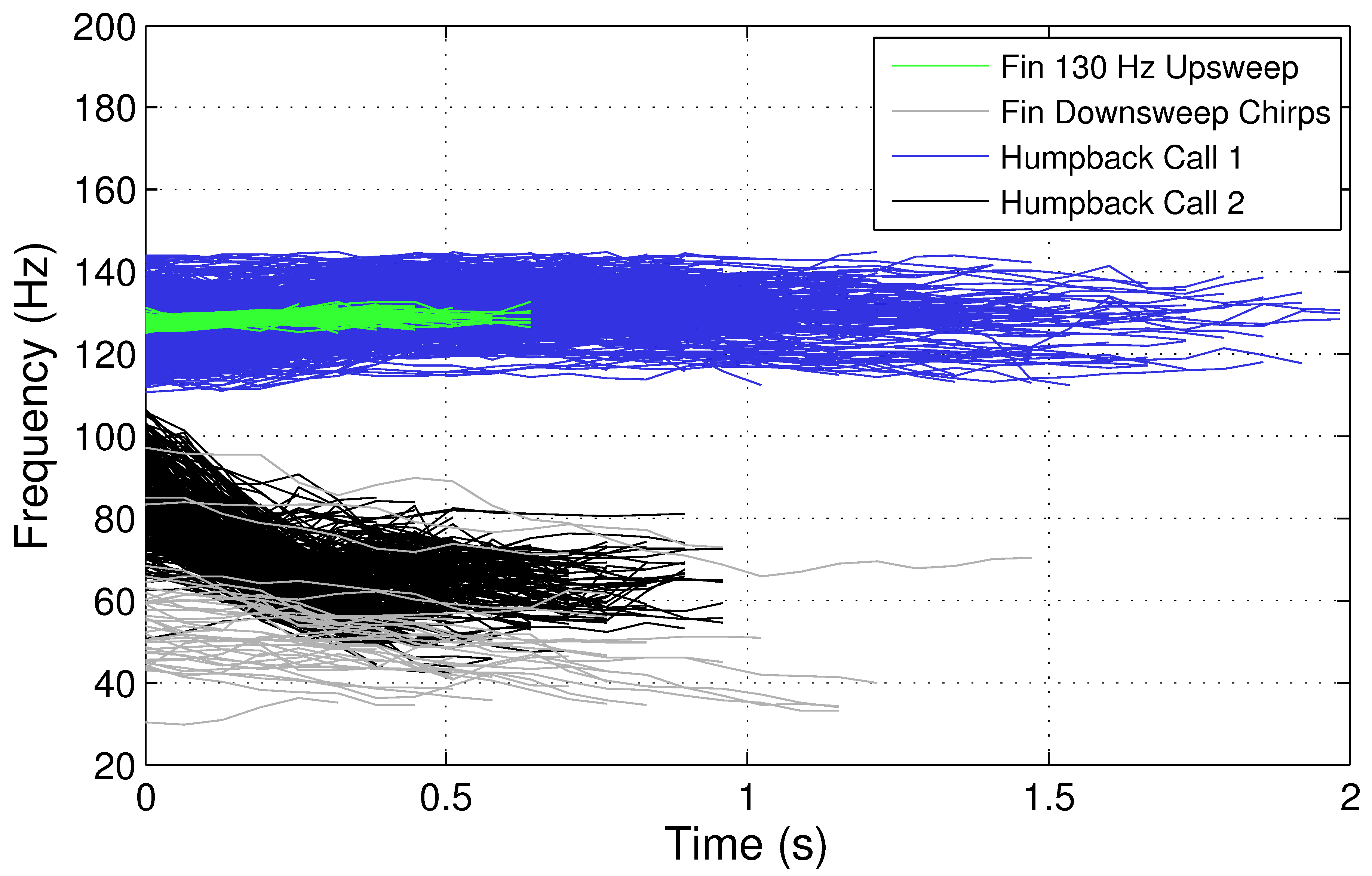
One of the challenges of developing an automatic classifier for near real-time fin whale vocalization detection from acoustic spectrograms, is the ability to differentiate fin whale vocalizations from other biological and man-made acoustic sound sources. Figure 2 displays examples of several common acoustic signals and sound sources observed during the Norwegian Sea Experiment 2014 (NorEx14) [1] in the frequency range of fin whale vocalizations, which include seismic airgun, ship tonal, and humpback whale vocalization signals. Unfortunately, many of these signals have overlapping features, such as bandwidth, with specific types of fin whale vocalizations that may cause ambiguity in identification. As an example, Figure 3 compares the pitch-tracks for two types of humpback whale vocalizations with the fin whale 130 Hz upsweep and 30–100 Hz downsweeps. As indicated in Figure 3, the humpback whale vocalizations appear to have some similar time–frequency characteristics as the fin whale 130 Hz upsweep and 30–100 Hz downsweeps, and it may be challenging to correctly classify these two types of fin whale vocalizations from humpback whales vocalizing in the same region, depending on the classification method utilized. Therefore, a robust classification system is necessary to enable the fin whale 20 Hz pulse, 130 Hz upsweep, backbeat pulse, and 30–100 downsweep chirp vocalizations to be recognized and differentiated from other acoustic sound sources.

Here, a large training data set of fin whale vocalization and other acoustic signal detections are gathered after manual inspection and labeling. The fin whale vocalizations were identified by first clustering all the detected acoustic signals, on a specific observation day, using various time–frequency features and unsupervised clustering algorithms described in Section 2.2. Each cluster was then manually inspected to positively label a cluster as containing fin whale vocalization detections. This was accomplished by visually reviewing the spectrograms and time–frequency characteristics associated with the detected acoustic signals from each cluster. As a final step, each cluster identified as containing fin whale vocalization detections was filtered manually to eliminate non-fin whale vocalization detections [1]. This approach gave us the capability to analyze and identify marine mammal vocalizations that have not been previously documented or observed, by associating bearing-time trajectories of unknown acoustic sound sources with known acoustic sound sources. However, manual filtering is not a viable method of identifying fin whale vocalizations for real-time applications given the long time duration needed for the analysis and limited number of trained individuals with experience to visually identify different types of fin whale vocalizations from spectrograms. Therefore, it is essential to develop an automatic classifier for real-time fin whale vocalization detection applications.

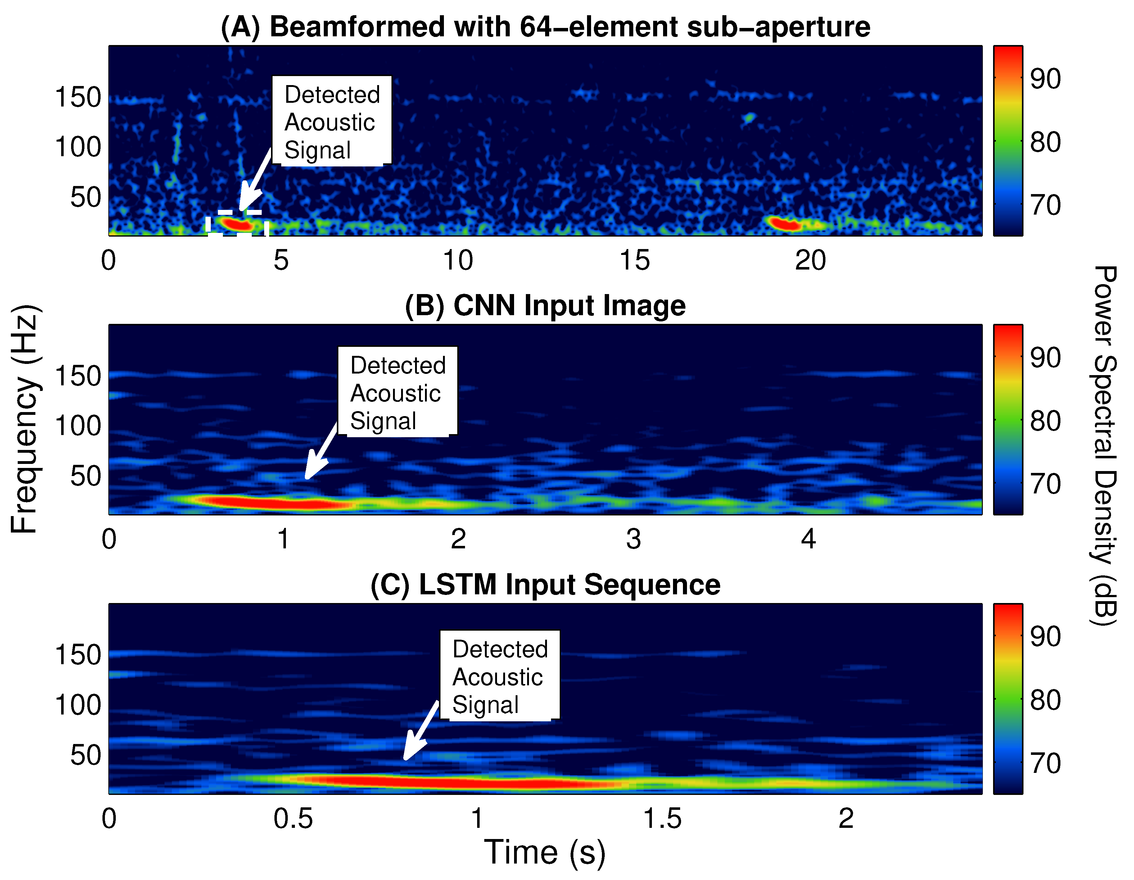
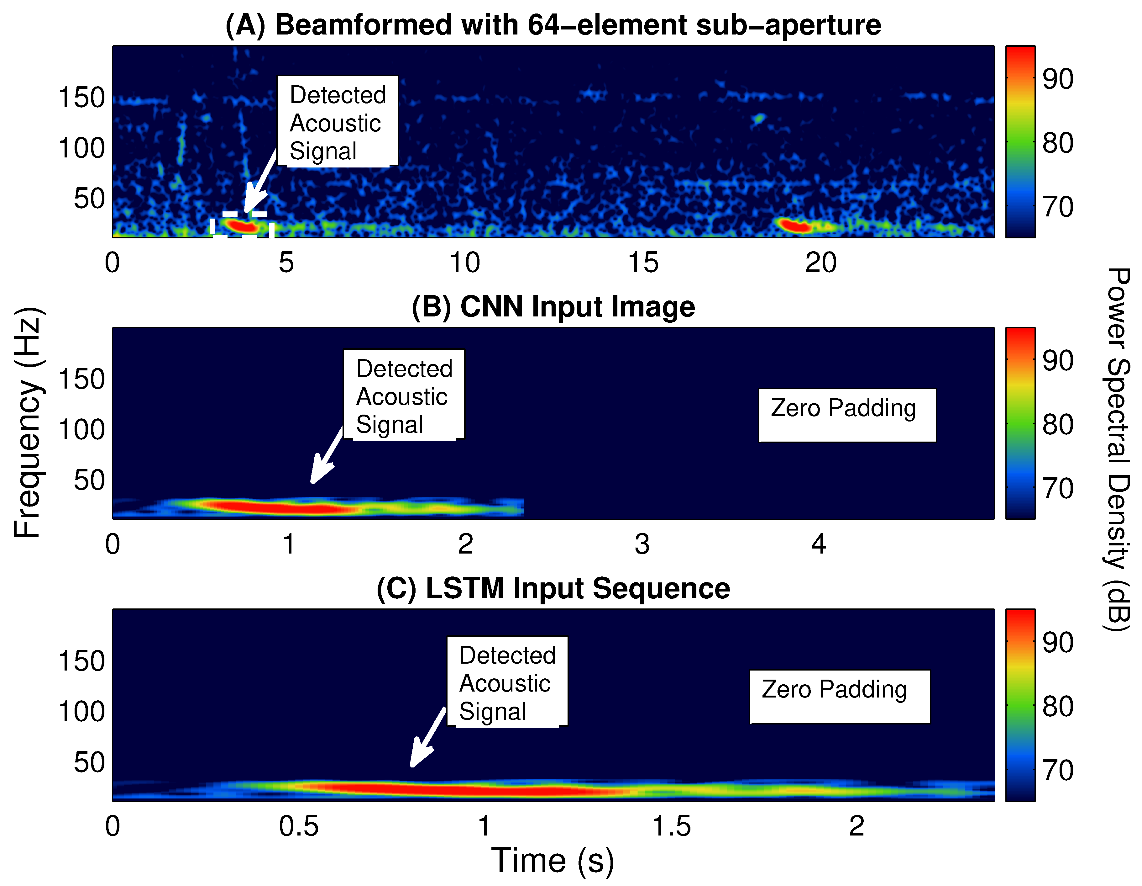
Multiple classifiers, including a logistic regression, SVM, decision tree [19], CNN [20,21,22], and LSTM network [23], are built and tested for identifying fin whale vocalizations from the enormous amount of acoustic signals detected by POAWRS per day. Here, the CNN and LSTM classifiers are trained using beamformed spectrogram images as inputs to classify each detected acoustic signal, while logistic regression, SVM and decision tree classifiers are trained using 12 features extracted from each detected acoustic signal in a beamformed spectrogram. The performance of the classifiers are evaluated and compared using multiple metrics including accuracy, precision, recall and F1-score. The last step includes integrating one of the classifiers into the existing POAWRS array and signal processing software to provide an automatic classifier for near real-time fin whale monitoring applications. The classifiers developed here can enable near real-time identification of fin whale vocalization signal types since the classification run time is found to be on the order of seconds, given tens to hundreds of thousands of input signals received by the coherent hydrophone array. The fin whale vocalization classifier presented, here, will lay the foundation for building an automatic classifier for near real-time detection and identification of various other biological, geophysical, and man-made sound sources in the ocean.

Automatic classification approaches, including machine learning, can help to efficiently and rapidly classify ocean acoustic signals according to sound sources in ocean acoustic data sets within significantly reduced time frames. Various automatic classification techniques have been applied for ocean biological sensing from animal vocalizations and sounds received on both single hydrophone and coherent hydrophone arrays [9,24,25]. In [26], the performance of Mel Frequency Cepstrum Coefficients (MFCC), the linear prediction coding (LPC) coefficients, and Cepstral coefficients for representing humpback whale vocalizations were explored, and then K-means clustering was used to cluster units and subunits of humpback whale vocalizations into 21 and 18 clusters, respectively. The temporal and spatial statistics of humpback whales song and non-song calls in the Gulf of Maine, observed using a large-aperture coherent hydrophone array, were quantified over instantaneous continental shelf scale regions in [9]. Subclassification of humpback whale downsweep moan calls into 13 sub-groups were accomplished using K-means clustering after beamformed spectrogram analysis, pitch-tracking and time–frequency feature extraction. Automatic classifiers were further developed in [24] to distinguish humpback whale song sequences from nonsong calls in the Gulf of Maine by first applying Bag of Words to build feature vectors from beamformed time-series signals, calculating both power spectral density and MFCC features, and then employing and comparing the performances of Support Vector Machine (SVM), Neural Networks, and Naive Bayes in the classification. Identification of individual male humpback whales from their song units was investigated in [27], via extracting Cepstral coefficients for features and then applying SVM for classification. In [28], blue whale calls were classified using neural network with features derived from short-time Fourier and wavelet transforms. In [29], an automatic detection and classification system for baleen whale calls was developed using pitch tracking and quadratic discriminant function analysis. Echolocation clicks of odontocetes were classified by exploiting cepstral features and Gaussian mixture models in [30], while in [31], whale call classification was accomplished using CNNs and transfer learning on time–frequency features. Fish sounds were classified using random forest and SVM in [32].

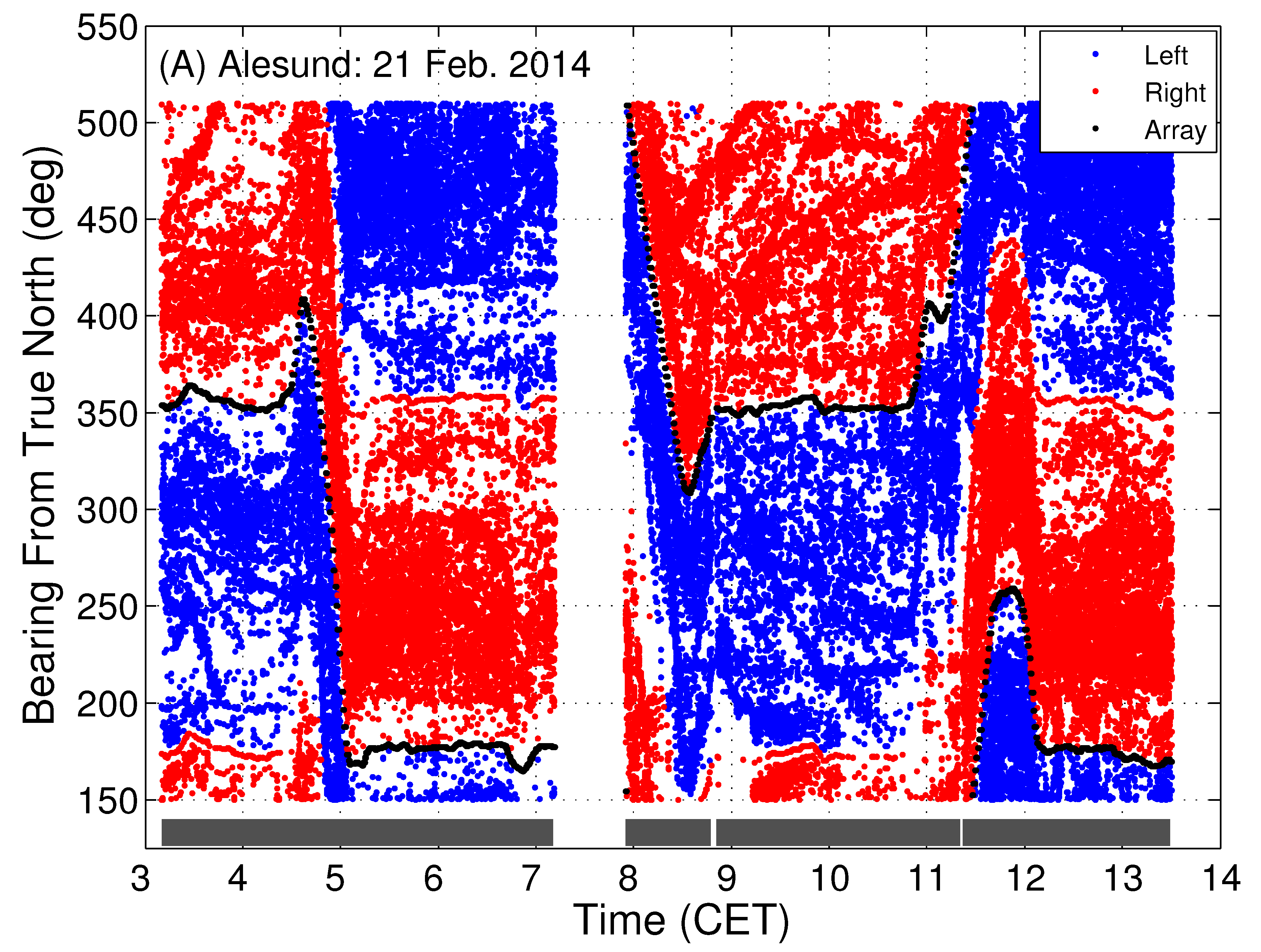
Here, the automatic classification and machine learning algorithms are applied to large-aperture coherent hydrophone array data, where the input to the classifiers are beamformed data in the form of beamformed frequency-time spectrograms or extracted features, or beamformed time-series, spanning all 360 degrees horizontal azimuth about the coherent hydrophone array. The output of the classifier therefore provides identification of fin whale call types spatially distributed across multiple bearings from the receiver array. The identified fin whale vocalization bearing-time trajectories are required for spatial localization and horizontal positioning of fin whales [1].

2. Materials and Methods

2.1. Measurement of Fin Whale Vocalizations Using a Coherent Hydrophone Array

The underwater recordings of fin whale vocalizations analyzed here are drawn from the NorEx14, conducted by a collaborative team from the Massachusetts Institute of Technology, Northeastern University, NOAA-Northeast Fisheries Science Center, Naval Research Laboratory, Penn State University and the Woods Hole Oceanographic Institution in the United States, as well as the Institute of Marine Research-Bergen (IMR) in Norway. The NorEx14 was conducted from 18 February to 8 March 2014, in conjunction with the IMR survey of spawning populations of Atlantic herring off the Alesund coast, the Atlantic cod off the Lofoten peninsula, and the capelin off the Northern Finnmark region [33,34]. The twofold objectives of the NorEx14 were to (i) image and monitor the population distributions of these large fish shoals from diverse species instantaneously over wide areas of their spawning grounds, using the Ocean Acoustic Waveguide Remote Sensing (OAWRS) and imaging system [33,35,36,37] from which fish group behavioral patterns can be quantified, and (ii) observe marine mammal vocalizations and infer their temporal–spatial distributions over wide areas using the POAWRS technique, [1,2,9,11] combined with visual observations for species confirmation. The marine mammal vocalization data, that include fin whale vocalizations obtained from POAWRS sensing, were partially processed at sea and further analyzed in post-processing.

In NorEx14, recordings of underwater sound were acquired using a horizontal coherent hydrophone array [38] towed at an average speed of 4 knots (~2 m/s) along designated tracks for 8–24 h per day. To minimize the effect of tow ship noise on the recorded acoustic data, the coherent hydrophone array was towed approximately 280–330 m behind the research vessel so as to confine this noise to the forward endfire direction of the array, which is the forward direction parallel to the array axis. The tow ship noise in directions away from the forward endfire was negligible after coherent beamforming. The water depth ranged from 100 m to 300 m at the array locations, and the array tow depth varied from 45 to 70 m in NorEx14.

The multiple nested subapertures of the array contain a total of 160 hydrophones spanning a frequency range from below 10 Hz to 4000 Hz for spatially unaliased sensing. The mean sensitivity of each hydrophone is a constant in this frequency range. A fixed sampling frequency of 8000 Hz was used so that acoustic signals with frequency contents up to 4000 Hz were recorded without temporal aliasing. The ultra low-frequency (ULF) subaperture of the array consisting of 64 equally spaced hydrophones with inter-element spacing of 3 m, was used here to collect fin whale vocalizations with frequency content below 250 Hz. The horizontal beamwidth of the array is a function of the array aperture length L, steering angle $\varphi$, as well as center frequency $f_c$ and bandwidth B of the signal [39,40,41]. The 1 dB angular width ${\beta }_{1dB}(\varphi ,f_c)$ [10] of the receiver array for the fin whale 20 Hz pulse and 130 Hz upsweep vocalizations are provided in

Table 1. POAWRS receiving array 1-dB angular width ${\beta }_{1dB}(\varphi ,f_c)$ at broadside $(\varphi =0)$ and endfire $(\varphi =\pi /2)$, given ULF aperture length L, as a function of center frequency $f_c$ for a given fin whale call type. The amplitude weighted average frequency values in Table 2 of [1] were used as the center frequency values. A Hanning spatial window is applied in the beamforming.

Fin Whale	${\mathit{f}}_{\mathit{c}}$	L	${\mathit{\beta }}_{1\mathit{dB}}(\mathit{\varphi }=0)$	${\mathit{\beta }}_{1\mathit{dB}}(\mathit{\varphi }=\mathit{\pi }/2)$
Call Type	(Hz)	(m)	(deg)	(deg)
20 Hz pulse	21.5	189	10	19.5
130 Hz upsweep	128.7	189	1.7	8

. The steering angle $\varphi$ is measured as the horizontal azimuthal angle from array broadside. The bearing estimation errors are significantly smaller by a factor of roughly 1/5 for the fin whale 130 Hz upsweep signals in comparison to the 20 Hz pulse signals after beamforming with the ULF subaperture.

Physical oceanography was monitored by sampling water column temperature and salinity with expendable bathythermographs (XBTs) and conductivity–temperature–depth (CTD) sensors at regular intervals of a couple of hours each day. The water column sound speed profile measured in the three distinct regions of the Norwegian Sea are provided in [42].

The detection of long-range propagated sounds is significantly enhanced by spatial beamforming and spectrogram analysis which filters the background noise that is outside of the beam and frequency band of the fin whale vocalizations. The high gain [39,43] of the coherent 64-hydrophone ULF subaperture, of up to $10{log}_{10}64=$ 18 dB, enabled detection of fin whale vocalizations up to two orders of magnitude more distant in range in the shallow water environment than a single omnidirectional hydrophone, which has no array gain (see Figure 2 of [1]). The actual array gain, which may be smaller than the full 18 dB array gain, is dependent on noise coherence and vocalization wavelength relative to array aperture length. For example, the array gain for the 20 Hz pulse is 5.3 dB, while the array gain for the 130 Hz upsweep is 13.7 dB due to the difference in wavelengths of the signals.

The POAWRS coherent hydrophone array employed in NorEx14 detected significant sounds from a wide range of underwater acoustic sources including marine mammal vocalizations from diverse baleen and toothed whale species in the frequency range from 10 Hz up to 4 kHz, and sounds from a large number of diesel–electric surface ships and other powered ocean vehicles [12]. Here the analysis is focused on the detection and classification of fin whale vocalizations between the 10–200 Hz frequency range. Concurrent ship-based visual observations conducted during our experiment provides confirmation of the presence of fin whales.

2.2. Fin Whale Vocalization Detection and Identification

Acoustic pressure–time series measured by sensors across the receiver array were converted to two-dimensional beam-time series by discrete Fourier transform [44]. A total of 64 beams were formed spanning 360 degree horizontal azimuth about the receiver array for data from the ULF subaperture. Each beam-time series was converted to a beamformed spectrogram by short-time Fourier transform (sampling frequency = 8000 Hz, frame = 2048 samples, overlap = 3/4, Hann window). Significant sounds present in the beamformed spectrograms were automatically detected by first applying a pixel intensity threshold detector [45] followed by pixel clustering, and verified by visual inspection [2,8,9,12]. Beamformed spectrogram pixels with local intensity values that are 5.6 dB above the background are grouped using a clustering algorithm according to a nearest-neighbour criteria that determines if the pixels can be grouped into one or more significant sound signals. Each individual detected signal is next characterized by its pitch track [29,46,47] representing the time variation of the fundamental frequencies. The pitch-track is estimated using a time–frequency peak detector from a signal’s detected and clustered pixel intensity values in the beamformed spectrogram.

The time–frequency characteristics of each individual detected signal is determined from its pitch-track. The pitch-track for a signal contains a time series $t=(t_1,t_2,\dots ,t_i)$, a frequency series $f=(f_1,f_2,\dots ,f_i)$, and an amplitude series $A=(A_1,A_2,\dots ,A_i)$ describing the time-variation of the fundamental frequency in the signal [29,46,47]. Eight features are extracted from each signal. They are (1) minimum frequency (Hz), $f_L$; (2) maximum frequency (Hz), $f_U$; (3) amplitude weighted average frequency (Hz), $\overline{f}$; (4) mean instantaneous bandwidth (Hz), $\overline{B}$; (5) relative instantaneous bandwidth, $\overline{B}/\overline{f}$; (6) duration (s), $\tau =t_i-t_1$; (7) slope from first-order polynomial fit (Hz/s), $\frac{df}{d\tau }$; and (8) curvature from second-order polynomial fit (Hz/s${}^2$), $\frac{d^{2}f}{d{\tau }^2}$. The slope and curvature are obtained from second-order nonlinear curve fit to the vocalization traces obtained via pitch-tracking [2,9].

The time–frequency characteristics extracted via pitch-tracking are applied for identifying fin whale vocalizations. First, a combination of extracted features from pitch-tracking, orthogonalized via principal component analysis (PCA) [48], were used to optimize the vocalization classification employing k-means [49] and Bayesian-based Gaussian mixture model clustering approaches [50]. The number of clusters can be determined via Bayesian information criterion (BIC) [51]. Clusters containing fin whale vocalization types were positively identified and labeled using the cluster-averaged time–frequency features, and verified by visual inspection of all pitch tracks grouped into clusters, as well as select spectrograms. The bearing-time trajectories of each closely associated series of vocalizations were also taken into account to ensure consistent classification [9].

2.3. Algorithms for Automatic Fin Whale Vocalization Classification

Multiple classification algorithms were considered for identifying the 20 Hz pulse (single), 20 Hz pulse (doublet), 130 Hz upsweep, backbeat pulse, and 30–100 Hz downsweep chirps from other acoustic signals. The classification algorithms include logistic regression, SVM, decision tree, CNN, and LSTM. A comprehensive review of these classification algorithms, their theoretical limits, and performance bounds can be found in [19] for logistic regression, SVM, and decision tree; [20,21,22] for CNN; and [23] for LSTM.

All of the classifiers were implemented via Matlab on a single Intel Xeon processor with 4 cores operating at 3.7 GHz and 64 GB of RAM, equipped with a NVIDIA Quadro K620 2GB GPU. The training data for the logistic regression, SVM, and decision tree classifiers were split into training (70%) and validation (30%) data using Matlab functions. The Matlab functions also automatically perform hyperparameter optimization for these classifiers to prevent overfitting and underfitting. Hyperparameters optimized by Matlab in these classifiers are provided in [52].

The CNN architecture consisted of an input layer with dimensions of the image size (194 × 79), three sets of n convolutional layers with m filters, each followed by batch normalization and ReLU activation functions. The n and m are hyperparameters, where the bounds for n is 1 to 3 and the bounds for m is 9 to 32. Each of these three sets was followed by a 2 by 2 max pooling layer. Finally, we used a fully connected layer, softmax layer, and classification layer in the output. The hyperparameters were optimized to be $n=2$ and $m=22$.

The LSTM architecture consisted of an input layer with dimensions of the image size (194 $\times N$), where N is the number of time indices determined by the time duration of the acoustic signal. The max size of N was set to 79 due to memory constraints. The hidden unit ranged from 100 to 3000 and was optimized to 500. We used a fully connected layer, softmax layer, and classification layer in the output.

The runtimes for training the logistic regression, SVM, and decision tree classifiers were on the order of a few minutes, whereas the classification of test data completed in a second. For the CNN and LSTM classifiers, the training runtimes were on the order of several hours, while the classification of test data completed on the order of a few seconds. The test data comprises of roughly 10 h of coherent hydrophone array recording where the signal detections are classified on the order of a few seconds or less for fin whale vocalization types. Incoming POAWRS data files of roughly 1 min duration will require much less time, making real-time classification attainable.

2.4. Training and Test Data Set

The CNN and LSTM classifiers are trained and tested using beamformed spectrogram images of acoustic signal detections as inputs, whereas logistic regression, SVM, and decision tree classifiers are trained and tested using 12 features extracted from each acoustic signal detection in beamformed spectrograms. Note that the SVM classifier can also be trained using images [53,54,55] as input, such as beamformed spectrogram images, and will be investigated in future work.

Each of the classification algorithms were used to develop a fin whale vocalization classifier (ref). The training and test data sets for each classifier were extracted from a subset of POAWRS detections observed during the NorEx14, and outlined in

Table 2. Training data set was extracted from a subset of POAWRS detections within the 10–200 Hz frequency range, observed off the coast of Alesund, Norway on 19–20 February 2014; off the coast of Northern Finnmark, Norway on 26 February 2014; and off the coast of Lofoten, Norway on 5 March 2014. Note that the total number of non-fin whale (Class 6) detections is significantly larger when going up to the 4 kHz frequency range since this training set is only a subset of the overall POAWRS detections on each day. (* The number of calls could not be confidently estimated (NA, not accessible) for the 20 Hz pulse (doublet), downsweep chirps, and backbeats measured off the coast of the Northern Finnmark region on 26 February 2014 due to multiple known and unknown marine mammal species vocalizing in close proximity and in the same frequency band).

		Training	(Class 1)	(Class 2)	(Class 3)	(Class 4)	(Class 5)	(Class 6)
Day	Audio	Data	20 Hz	20 Hz	130 Hz	Backbeat	Downsweep	Non-fin
	(h)	Set	Pulse	Pulse	Pulse		Chirps	Whale
			(Single)	(Doublet)	Upsweep
19 Feb	21	No. of calls	4575	1235	574	426	0	109,980
		% trained	100	100	100	100	0	100
20 Feb	22.4	No. of calls	6880	1002	1454	325	39	95,663
		% trained	100	100	100	100	100	100
26 Feb	6.3	No. of calls	10,768	* NA	8666	* NA	* NA	18,096
		% trained	0	0	64	0	0	0
05 Mar	6.1	No. of calls	881	6	337	1	0	31,936
		% trained	0	0	0	0	0	12
Total No. trained			11,455	2237	7546	751	39	209,555

and

Table 3. Test data set was extracted from a subset of POAWRS detections within the 10 to 200 Hz frequency range and observed off the coast of Alesund, Norway on 21 February 2014. It should be noted that the total number of non-fin whale (Class 6) detections is significantly larger when going up to the 4 kHz frequency range since this data set is only a subset of the overall POAWRS detections on 21 February 2014.

		Testing	(Class 1)	(Class 2)	(Class 3)	(Class 4)	(Class 5)	(Class 6)
Day	Audio	Data	20 Hz	20 Hz	130 Hz	Backbeat	Downsweep	Non-fin
	(h)	Set	Pulse	Pulse	Pulse		Chirps	Whale
			(Single)	(Doublet)	Upsweep
21 Feb	21.6	No. of calls	985	1041	836	171	0	40,761
		% tested	100	100	100	100	0	100
Total No. tested			985	1041	836	171	0	40,761

. Each POAWRS detection in the training and test data set was visually inspected, verified, and given a classification label between 1 and 6, where the six different classes are defined as (1) 20 Hz pulse (single), (2) 20 Hz pulse (doublet), (3) 130 Hz upsweep, (4) backbeat pulse, (5) 30–100 Hz downsweep chirp, and (6) non-fin whale vocalization. Note that only the POAWRS detections between the frequency range 10–200 Hz will be utilized for this analysis, since the fin whale vocalizations identified in Figure 1 are within this frequency range.

As displayed in Table 2, the training data set was extracted from observation days on 19–20 February 2014, 26 February 2014, and 5 March 2014 during the NorEx14. The observation days on 19–20 February 2014 were chosen because there were a variety of different types of fin whale vocalizations present. There were also a variety of acoustic sound sources within the same frequency range as the fin whale vocalizations observed, such as the humpback whale vocalizations, seismic airgun signals, and ship tonals. The training data extracted from the observation day on 26 February 2014 contained significant amounts of fin whale 130 Hz upsweeps, whereas the observation day on 5 March 2014 contained humpback whale vocalizations (labeled as class 6). The training data from 26 February 2014 and 5 March 2014 were added to increase the number of training data examples for those two types of specific vocalizations and improve overall classification performance.

As displayed in Table 3, the test data set was extracted from the observation day on 21 February 2014 during the NorEx14. As with the training data set, this observation day was chosen because there was a variety of different types of fin whale vocalizations and acoustic sound sources within the same frequency range as the fin whale vocalizations observed. The bearing-time trajectories for 21 February 2014 are displayed in Figure 4 and show a total of 43,794 POAWRS detections, between the 10 and 200 Hz frequency range, in an approximate nine hour window of passive acoustic monitoring. In addition, only 3033 out of the 43,794 POAWRS detections have been identified as fin whale vocalizations. Visual inspection of Figure 4 shows a dense amount of acoustic signals arriving from a wide range of bearings relative to the coherent hydrophone array, which presents a potentially challenging classification environment for the five classification algorithms that will be tested here. Unfortunately, there were no 30–100 Hz downsweep chirps observed on this specific day. However, we still have the ability to evaluate if there are false alarms due to any acoustic signals (such as humpback whale vocalizations) being misclassified as a 30–100 Hz downsweep chirp.

2.4.1. Feature Data for Logistic Regression, SVM, and Decision Tree Classifiers

For each acoustic signal in the training and test data sets (see Table 2 and Table 3), twelve features were extracted to train and test the logistic regression, SVM, and decision tree classifiers. For ten of the features, the time–frequency characteristics of each individual acoustic signal are estimated by using its pitch-track. As mentioned in Section 2.2, the pitch-track for a signal contains a time series $t=(t_1,t_2,\dots ,t_i)$, a frequency series $f=(f_1,f_2,\dots ,f_i)$, and an amplitude series $A=(A_1,A_2,\dots ,A_i)$ describing the time-variation of the fundamental frequency in the signal [29,46,47]. The ten features are (1) minimum frequency (Hz), $f_L$; (2) maximum frequency (Hz), $f_U$; (3) average frequency (Hz), ${\overline{f}}_A$; (4) amplitude weighted average frequency (Hz), $\overline{f}$; (5) maximum bandwidth (Hz), $B_U$; (6) mean instantaneous bandwidth (Hz), $\overline{B}$; (7) relative instantaneous bandwidth, $\overline{B}/\overline{f}$; (8) duration (s), $\tau =t_i-t_1$; (9) slope from first order polynomial fit (Hz/s), $\frac{df}{d\tau }$; and (10) curvature from second order polynomial fit (Hz/s${}^2$), $\frac{d^{2}f}{d{\tau }^2}$. The last two features are (11) a rough estimate of the mean instantaneous SNR, ${\overline{I}}_{SNR}$, and (12) total number of time–frequency pixels that the detected acoustic signal from the beamformed spectrogram occupies, $P_x$. It is worth noting that eight of the twelve features were used in the time–frequency characterization of the fin whale vocalizations in Section 2.2. The other four features were included to potentially improve fin whale classification performance.

Next, we would like to gain some insights into which of the 12 features, as listed in Section 2.4.1, extracted from the feature data in the training data set (see Table 2), have the most significant variation or weight between the six classes defined in Section 2.4. This is accomplished by employing PCA [48] to understand the relationship between the 12 features and the principal components (PCs) [56,57]. Here, the feature data is given by $X=(x_1,\dots ,x_N)$, where $x_i$ is a M-dimensional vector measurement with each dimension corresponding to a given feature ($M=12$), N is the observation number (N = 231,583), and the PCs are defined as the eigenvalues of the covariance matrix, $cov\left(X\right)$. For each PC, the components of its eigenvector measure the contributions from each of the 12 features.

In Figure 5A, the PCs are normalized (by the sum of the eigenvalues) and ordered from highest to lowest (i.e., from most to least significant), which shows that PC1–PC3 occupies $99\%$ of the significance in comparison to PC4–PC12; PC1 occupies $86\%$ of the significance. Figure 5B–D display the normalized eigenvector components for PC1–PC3, measuring the contributions from each of the original 12 features. From Figure 5B and the $86\%$ significance of PC1, we find that the frequency information (original features (1–4)) provides the greatest differences across the training data set investigated. Therefore, the frequency information may have the most weight in classification performance using the logistic regression, SVM, and decision tree algorithms.

2.4.2. Image Data for CNN Classifier

For each training and test data set example in Table 2 and Table 3, an input image data structure was constructed to train and test the CNN classifier. The image was constructed by first creating an $M\times N$ matrix padded with zeros, where M is the total number of frequencies used in the beamformed spectrogram, and N is the number of time indices set by the user. Ideally, we would have set the image width N to accommodate the largest signal detected; however, for this analysis, N was set to 79, which equated to the first 5 s of the acoustic signal. This parameter was chosen because the duration of the fin whale vocalizations identified in Figure 1 are all less than 5 s, and we are also limited by the random access memory storage capacity in our current computer systems. As a final step, the portion of the beamformed spectrogram that coincides with the frequency range and the first 5 s of the detected acoustic signal was inserted into the $M\times N$ matrix. Figure 6B shows an example of a CNN input data image for a single fin whale 20 Hz pulse detection.

2.4.3. Time Series Data for LSTM Classifier

For each training and test data set example in Table 2 and Table 3, a data sequence time series was generated to train and test the LSTM classifier, constructed similarly to the images in Section 2.4.2. The time series data was constructed by first creating an $M\times N$ matrix padded with zeros, where M is the total number of frequencies used in the beamformed spectrogram, and N is the number of time indices determined by the time duration of the acoustic signal. As a final step, the portion of the beamformed spectrogram that coincides with the frequency range and time duration of the detected acoustic signal was inserted into the $M\times N$ matrix. Figure 6C shows an example of a data sequence time series for a single detected fin whale 20 Hz pulse. For this application, each $M\times N$ matrix is viewed as a sequence containing M features and varies with length.

2.5. Classifier Performance Evaluation

The performance of each classifier will be evaluated and compared using multiple metrics, which include accuracy, precision, recall, and F1-score. The metrics are defined as follows.

$$\begin{array}{c}\hfill \mathrm{total}\mathrm{accuracy}=\frac{\mathrm{total}\mathrm{number}\mathrm{of}\mathrm{true}\mathrm{positives}\left(\mathrm{all}\mathrm{classes}\right)}{\mathrm{total}\mathrm{number}\mathrm{of}\mathrm{observations}}\end{array}$$

(1)

$$\begin{array}{c}\hfill \mathrm{fin}\mathrm{accuracy}=\frac{\mathrm{total}\mathrm{number}\mathrm{of}\mathrm{true}\mathrm{positives}\left(\mathrm{all}\mathrm{fin}\mathrm{classes}\right)}{\mathrm{total}\mathrm{number}\mathrm{of}\mathrm{fin}\mathrm{observations}}\end{array}$$

(2)

$$\begin{array}{c}\hfill \mathrm{precision}=\frac{\mathrm{true}\mathrm{positive}\left(\mathrm{class}\right)}{\mathrm{number}\mathrm{of}\mathrm{predictive}\mathrm{positives}\left(\mathrm{class}\right)}\end{array}$$

(3)

$$\begin{array}{c}\hfill \mathrm{recall}=\frac{\mathrm{true}\mathrm{positive}\left(\mathrm{class}\right)}{\mathrm{number}\mathrm{of}\mathrm{actual}\mathrm{positives}\left(\mathrm{class}\right)}\end{array}$$

(4)

$$\begin{array}{c}\hfill \mathrm{F}1-\mathrm{score}=2\times \frac{\mathrm{precision}\times \mathrm{recall}}{\mathrm{precision}+\mathrm{recall}}\end{array}$$

(5)

The total accuracy of the classifier incorporates the true positives from all the classes and quantifies the overall ratio of correctly classifying all the observations in the test data set. In contrast, the fin accuracy incorporates the true positives from all the fin whale vocalization classes and quantifies the overall ratio of correctly classifying all the fin whale vocalization observations in the test data set. The precision metric is important because it quantifies how well the classifier will avoid false positives for a specific type of class. The recall metric is important because it quantifies how well the classifier will predict true positives for a specific type of class. The F1-score is a weighted average of precision and recall and helps consolidate the two metrics.

3. Results

3.1. Classification Confusion Matrices

The logistic regression, SVM, decision tree, CNN, and LSTM classifiers were trained using the data set identified in Table 2 and tested using data set identified in Table 3. The results from each of the five types of fin whale classifiers are provided in the confusion matrices displayed in

Table 4. Confusion matrix displaying results from the logistic regression classifier. The green highlighted numbers are true positives, and the red highlighted numbers are false positives.

,

Table 5. Confusion matrix displaying results from the SVM classifier. The green highlighted numbers are true positives, and the red highlighted numbers are false positives.

,

Table 6. Confusion matrix displaying results from the decision tree classifier. The green highlighted numbers are true positives, and the red highlighted numbers are false positives.

,

Table 7. Confusion matrix displaying results from the CNN classifier. The green highlighted numbers are true positives, and the red highlighted numbers are false positives.

and

Table 8. Confusion matrix displaying results from the LSTM classifier. The green highlighted numbers are true positives, and the red highlighted numbers are false positives.

. Each confusion matrix provides the classification results for six types of classes, which are defined as (1) 20 Hz pulse (single), (2) 20 Hz pulse (doublet), (3) 130 Hz upsweep, (4) backbeat pulse, (5) 30–100 Hz downsweep chirps, and (6) non-fin whale vocalizations. In addition, the green highlighted numbers are true positives, and the red highlighted numbers are false positives.

3.2. Classifier Accuracy

The classifier accuracy results are provided in

Table 9. Classifier accuracy results.

Accuracy	Logistic	SVM	Decision	CNN	LSTM
	Regression		Tree
Total	0.969	0.986	0.987	0.964	0.951
Fin	0.771	0.908	0.897	0.760	0.540

. The results were calculated using the information from each of the confusion matrices displayed in Table 4, Table 5, Table 6, Table 7 and Table 8. The total accuracy metric (see Equation (1)) represents the total number of correctly classified acoustic signals divided by the total number of acoustic signals from the test data set in Table 3. Here, the total accuracy results are all greater than $95\%$ for each of the classifiers investigated, which shows that a great majority of the 43,794 acoustic signals in Table 3 were classified correctly. The fin accuracy results are given in Table 9, where the fin accuracy (see Equation (2)) represents the total number of correctly classified fin whale vocalizations divided by the total number of fin whale vocalizations from the test data set in Table 3. Here, the fin accuracy results show a larger variation than the total accuracy results. The SVM classifier had the largest value of approximately $91\%$, whereas the LSTM classifier had the smallest value of $54\%$. The SVM and decision tree classifiers all had fin accuracy values greater than $89\%$, and both values were approximately within 1 percent from each other. The precision, recall and F1-score metrics will now be used in the next section to measure how well individual fin whale call types are classified from other fin whale and non-fin vocalizations, since both the total accuracy and fin accuracy metrics do not capture those individual classification quantities.

3.3. Classifier Precision, Recall, and F1-Score

The precision and recall results are provided in

Table 10. Classifier precision results.

Class	Logistic	SVM	Decision	CNN	LSTM
	Regression		Tree
1	0.762	0.806	0.879	0.532	0.497
2	0.909	0.970	0.986	0.821	0.852
3	0.838	0.840	0.914	0.707	0.575
4	0.257	0.871	0.926	0.795	0.792
5	NA	NA	NA	NA	NA
6	0.986	0.996	0.994	0.989	0.973

and

Table 11. Classifier recall results.

Class	Logistic	SVM	Decision	CNN	RNN
	Regression		Tree
1	0.903	0.907	0.898	0.702	0.429
2	0.865	0.897	0.862	0.787	0.485
3	0.525	0.939	0.926	0.841	0.827
4	0.637	0.830	0.877	0.544	0.111
5	NA	NA	NA	NA	NA
6	0.984	0.992	0.997	0.980	0.981

. The results were calculated using the information from each of the confusion matrices displayed in Table 4, Table 5, Table 6, Table 7 and Table 8. As described in Section 2.5, the precision metric quantifies how well the classifier will avoid predicting a false positive, while the recall metric quantifies how well the classifier will predict a true positive in regards to a specific class or type of fin whale vocalization. The F1-score results are provided in

Table 12. Classifier F1-score results.

Class	Logistic	SVM	Decision	CNN	LSTM
	Regression		Tree
1	0.826	0.853	0.888	0.605	0.461
2	0.886	0.932	0.920	0.803	0.618
3	0.646	0.887	0.920	0.768	0.678
4	0.366	0.850	0.901	0.646	0.195
5	NA	NA	NA	NA	NA
6	0.985	0.994	0.995	0.984	0.977

and were calculated using both the precision and recall results. The F1-score results are used to evaluate and compare the performance between the logistic regression, SVM, decision tree, CNN, and LSTM classifiers in identifying a specific class or type of fin whale vocalization. For each class or type of fin whale vocalization in

Table 13. Classifier performance rankings.

Class	Logistic	SVM	Decision	CNN	LSTM
	Regression		Tree
1	3	2	1	4	5
2	3	1	2	4	5
3	5	2	1	3	4
4	4	2	1	3	5
5	NA	NA	NA	NA	NA
6	3	2	1	4	5
Total	18	9	6	18	24

, a classifier was ranked between 1 to 5, where a classifier with a rank of 1 had the largest F1-score, whereas a classifier with a rank of 5 had the smallest F1-score. The overall classifier ranking is calculated by summing up each column in Table 13 and ranking each classifier by the lowest total score.

As discussed in Section 2.4, there were no 30–100 Hz downsweep chirps in the test data set chosen for this analysis. Consequently, the precision, recall, F1-score, and performance ranking results for each of the five types of classifiers are listed as non-applicable (NA) for the 30–100 Hz downsweep chirp (Class 5) (see Table 10, Table 11, Table 12 and Table 13). This can be attributed to the calculated precision and recall results having either a NaN or 0 value for the 30–100 Hz downsweep chirp (Class 5) calculations (see Equations (3)–(5)). However, we still evaluated if there were false alarms due to any acoustic signals (such as humpback whale vocalizations) being misclassified as a 30–100 Hz downsweep chirp (Class 5). As displayed in each classifier confusion matrix (see Table 4, Table 5, Table 6, Table 7 and Table 8), the number of false alarms in classifying detections as the 30–100 Hz downsweep chirp (Class 5) were all less than 7, which shows that approximately less than 0.02% of the non-fin whale (Class 6) vocalizations were misclassified as a 30–100 Hz downsweep chirp (Class 5).

According to the Table 13, the decision tree classifier had the best overall ranking with a minimum total score of 6. As displayed in Table 12, the F1-score results for the decision tree classifier were all greater than approximately $89\%$ for the fin whale vocalization classes. The overall classifier rankings between the decision tree and SVM classifiers were fairly close with a total score of 6 for the decision tree classifier and a total score of 9 for the SVM classifier (see Table 13). As displayed in Table 12, the F1-scores from both of these classifiers were all greater than $85\%$ for the fin whale vocalization classes and less than $6\%$ from each other.

The logistic regression and CNN classifiers both had a total score of 18 for their overall classifier rankings. These results can be attributed to low F1-score values for the fin whale vocalization classes, which ranged from 37% to 89% for logistic regression and 61 to 80% for CNN, and were primarily caused by either a fin whale vocalization being misclassified as a non-fin whale (Class 6) vocalization or vice versa. As an example, using the logistic regression classifier results, the F1-score for the fin whale 130 Hz upsweep was 0.646, which was low due to the poor recall value of 0.525. The recall results can be explained by viewing the confusion matrix in Table 4, which shows that approximately $50\%$ of the 130 Hz upsweeps (Class 3) were misclassified as non-fin whale (Class 6) vocalization. Next, the F1-score for the fin whale backbeat (Class 4) was 0.366, which was substantially low due to the poor precision value of 0.257. The precision results can also be explained by viewing the confusion matrix in Table 4, which shows that approximately $73\%$ of the predicted backbeats from the logistic regression classifier were actually non-fin whale (Class 6) vocalizations. Therefore, by using the same methodology, the results from the CNN classifier shows approximately $33\%$ of the predicted 20 Hz pulses (single) (Class 1) were actually non-fin whale (Class 6) vocalizations and $40\%$ of the backbeats (Class 3) were misclassified as non-fin whale (Class 6) vocalizations.

The LSTM classifier had the worst overall ranking with a maximum total score of 24, where the F1-scores ranged between 20 and 68% for the fin whale vocalization classes. Here, the results from the LSTM classifier shows approximately $46\%$ of the 20 Hz pulses (single) (Class 1), $37\%$ of the 20 Hz pulses (doublet) (Class 2), and $86\%$ of the backbeats (Class 3) were misclassified as non-fin whale (Class 6) vocalizations. The results also show that approximately $35\%$ of the predicted 130 Hz upsweeps (Class 3) were actually non-fin whale (Class 6) vocalizations.

4. Discussion

4.1. Automatic Classifiers for Near Real-Time Fin Whale Applications

4.1.1. Decision Tree Classifier

The decision tree classifier may be a good potential candidate for near real-time fin whale vocalization detection application, because its F1-score results were all above $89\%$ for fin whale vocalization classes and it was ranked number 1 from the results in Table 12 and Table 13 for classifying fin whale vocalization detections. The set of 12 features for each acoustic signal detection is automatically calculated as a subroutine in our POAWRS processing software right after signal detection from beamformed spectrogram analysis, and therefore available for input to the classification algorithms.

As an example for demonstrating the feasibility for using a decision tree classifier for near real-time fin whale detection applications, we will again use the POAWRS detections from the NorEx14 on 21 February 2014 (see Table 3). Figure 7A displays the bearing-time trajectory results for all the acoustic signals detected between the 10 to 200 Hz frequency range, and, again, the results visually emphasize the significant amount of POAWRS detections on this observation day. Figure 7B displays the bearing-time trajectory results from the fin whale vocalization detections that were manually labeled and visually verified by the research team (which we can treat as providing “ground truth”), whereas Figure 7C only displays the fin whale vocalization detections that were identified by the decision tree classifier. Note that it took the research team approximately 2 full days to visually inspect and verify all the fin whale vocalization detections in each spectrogram from the test data set in Table 3, whereas it only took less than one second for the decision tree classifier to classify all 43,794 detections. A comparison of the data displayed in Figure 4B,C reveals that roughly $8\%$ (250) of the fin whale vocalization detections were misclassified as non-fin whale (Class 6) detections by the decision tree classifier, and therefore, were not included in Figure 4C. In addition, roughly $0.4\%$ (144) of the non-fin whale (Class 6) detections were misclassified as a specific type of fin whale vocalization by the decision tree classifier, and therefore, were included in Figure 4C. Interestingly, most of the misclassified 144 non-fin whale (Class 6) detections in Figure 4C appear like random noise in contrast to the denser tracks formed by the correctly classified fin whale vocalization detections. Therefore, misclassified non-fin whale (Class 6) detections may potentially be removed by an existing density-based spatial clustering algorithm, such as Density-Based Spatial Clustering of Applications with Noise (DBSCAN) [58].

The above analysis demonstrates the use of a decision tree classifier for rapid fin whale vocalization classification using 12 features extracted from each detection after beamformed spectrogram analysis of coherent hydrophone array data. Note that the volume of non-fin whale vocalization detections are typically larger by a factor of ten or more in the 10 Hz to 200 Hz frequency range, and arise due to other oceanic sound sources, such as other marine mammal species vocalizations, fish grunts, ship-radiated sound, other man-made sound sources, as well as unidentified sources. For simultaneously classifying these large categories of biological, geophysical and man-made sound sources, further training and testing with the five classifier approaches examined here, as well as other approaches will be neccessary in the future. Seasonal and regional trends and differences in the variety and abundance of ocean acoustic sound sources will also impact the performances of the classifiers.

As a final note, the bearing-time trajectories were used as one of the features to manually label the fin whale detections displayed in Figure 4B, but they were not included as a feature to train and test the decision tree classifier, SVM or logistic regression classifiers. Future work will incorporate the bearing-time trajectories of fin whale vocalization detections as potential feature to see if there is any increase in classification accuracy for each of the algorithms discussed here.

4.1.2. Neural Network Classifiers

As displayed in Table 12, the F1-scores from both the SVM and decision tree classifiers are all greater than $85\%$ for the fin whale vocalization classes, whereas the F1-scores for the CNN and LSTM classifiers ranged from 61 to 80% and 20 to 68%. Note that the reader should not conclude from this comparison that conventional classification algorithms (SVM and decision tree) are better than neural network classifiers (CNN and LSTM) for identifying fin whale vocalizations in beamformed spectrograms. Specifically, the performance results of the CNN and LSTM classifiers are preliminary, given that the CNN and LSTM classifier’s performance results may improve by modifying their input data structures or by optimizing the algorithm parameters. For example, the input data image for the CNN classifier and the input data sequence for the LSTM classifier were modified to only include the portion of the beamformed spectrogram that coincides with the detected acoustic signal as indicated in Figure 8b,c. The rest of the input image (CNN) or input data sequence (LSTM) that does not coincide with the detected acoustic signal is padded with zeros. This modification was performed to the CNN and LSTM input data structures to potentially increase classification performance by isolating each acoustic detected signal from the other acoustic signals contained in the input image (CNN) or input data sequence (LSTM).

The F1-score results from the CNN and LSTM classifiers using the modified input data structures are displayed in

Table 14. Fin whale classifier F1-score results (including results from the CNN and LSTM classifiers with modified input data structures).

Class	Logistic	SVM	Decision	CNN	CNN	LSTM	LSTM
	Regression		Tree		Modified		Modified
1	0.826	0.853	0.888	0.605	0.859	0.461	0.794
2	0.886	0.932	0.920	0.803	0.909	0.618	0.820
3	0.646	0.887	0.920	0.768	0.905	0.678	0.784
4	0.366	0.850	0.901	0.646	0.910	0.195	0.866
5	NA	NA	NA	NA	NA	NA	NA
6	0.985	0.994	0.995	0.984	0.995	0.977	0.991

, which includes the prior F1-scores from Table 12 for comparison. Here, the modification to the CNN input data structures improved the F1-scores for the fin whale vocalization classes by roughly 11–26% for the CNN classifier, which significantly impacted the overall ranking of the CNN classifier as displayed in

Table 15. Classifier performance rankings (Using the F1-scores from the CNN and LSTM classifiers with modified input data structures).

Class	Logistic	SVM	Decision	CNN	LSTM
	Regression		Tree	Modified	Modified
1	4	3	1	2	5
2	4	1	2	3	5
3	5	3	1	2	4
4	5	4	2	1	3
5	NA	NA	NA	NA	NA
6	4	2	1	1	3
Total	22	13	7	9	20

. Now, the overall rankings for the decision tree and CNN (using the modified input data structure) classifiers were fairly close with a total score of 7 for the decision tree classifier and a total score of 9 for the CNN classifier. As displayed in Table 14, the F1-scores from both of these classifiers were all greater than $85\%$ for the fin whale vocalization classes and less than 3% from each other. In addition, the modification to the LSTM input data structures improved the F1-scores for the fin whale vocalization classes by approximately 11–67% for the LSTM classifier, which significantly increased the classification performance (see Table 14). Here, the F1-scores for the LSTM (using the modified input data structure) classifier were all greater than $78\%$.

The previous example was just one proposed method to potentially increase the classification performance for both the CNN and LSTM classifiers for identifying fin whale vocalizations in beamformed spectrograms. Further research is required to investigate modifying other CNN and LSTM input data structure parameters such as the time duration, where we can utilize the information from the periodic nature and combinations of specific types of fin whale vocalizations to potentially increase classification performance. In addition, further research is required to investigate the optimization of the CNN and LSTM algorithm parameters, such as the number of hidden layers in the network, to potentially increase classification performance.

4.2. Building an Automatic Classifier for Near Real-Time Detection of Various Biological, Geophysical, and Man-Made Sound Sources

Ideally, we would like to build a classification system to identify every type of underwater acoustic signal detected during the NorEx14. The fin whale classifier developed in this journal article will provide a foundation and framework from which we will incorporate new classes of acoustic signals from training data acquired through future analyses. As an example, we identified and labeled 8952 detections of seismic airgun signals (see Figure 2) contained in the original training data set in Table 2, which were originally labeled as non-fin whale (Class 6) detections. In addition, we identified and labeled 822 detections of seismic airgun signals contained in the original test data set in Table 3, which were originally labeled as non-fin whale (Class 6) detections. Subsequently, we created a new class using the labeled seismic airgun signal detections known as Class 7. The updated training data set was then used to retrain the decision tree classifier. The results from the decision tree classifier, given the updated labels, is provided in the confusion matrix displayed in

Table 16. Confusion matrix displaying results from the decision tree fin whale classifier, given a new seismic airgun signal class (Class 7). The green highlighted numbers are true positives, and the red highlighted numbers are false positives.

, and the performance metrics displayed in

Table 17. Decision tree classifier performance results, given a new seismic airgun signal class (Class 7).

Class	Precision	Recall	F1-Score	Total	Fin
				Accuracy	Accuracy
1	0.873	0.888	0.881	0.987	0.879
2	0.965	0.842	0.899
3	0.874	0.915	0.894
4	0.926	0.883	0.904
5	NA	NA	NA
6	0.993	0.995	0.994
7	0.974	0.999	0.986

. The results show that the decision tree classifier’s F1-score results were above $88\%$ for all the classes. Furthermore, the decision tree classifier performance for classifying the seismic airgun signal detections (Class 7) was very good, with approximately a precision of $97\%$, a recall of $99\%$, and an F1-score of $98\%$. This example demonstrates the feasibility of adding and training new classes to the fin whale classifier to provide a fuller awareness of the acoustic sound sources in the ocean environment.

5. Conclusions

We considered five different types of classification algorithms to identify fin whale vocalizations: logistic regression, SVM, decision tree, CNN, and LSTM. The goal was to develop a fin whale classifier for near real-time fin whale detection applications. Each classifier was trained and tested using POAWRS detections from the NorEX14 data set. Each detection was categorized as either a specific type of fin whale vocalization or a non-fin whale vocalization. Further analysis will be required to identify the best classification approach for fin whale vocalizations due to challenges such as the limited size of the data set, which does not include the seasonal and regional differences in the acoustic signals detected. However, the decision tree classifier was ranked number 1 out of the five classifiers and has F1-score results all greater than $89\%$ from the current data set used.

The demonstrated performance of the decision tree classifier suggest that it is an excellent candidate to be applied for near-real time classification of fin whale detections for the Norwegian and Barents Seas. Ultimately, the fin whale classifier developed in this journal article will provide a framework for future development, such as incorporating new classes of acoustic signals from future collections of training data, as was shown here by incorporating detections of seismic airgun signals.

References

1. Garcia, H.A.; Zhu, C.; Schinault, M.E.; Kaplan, A.I.; Handegard, N.O.; Godø, O.R.; Ahonen, H.; Makris, N.C.; Wang, D.; Huang, W.; et al. Temporal–spatial, spectral, and source level distributions of fin whale vocalizations in the Norwegian Sea observed with a coherent hydrophone array. ICES J. Mar. Sci. 2018, 76, 268–283. [Google Scholar] [CrossRef]
2. Wang, D.; Garcia, H.; Huang, W.; Tran, D.D.; Jain, A.D.; Yi, D.H.; Gong, Z.; Jech, J.M.; Godø, O.R.; Makris, N.C.; et al. Vast assembly of vocal marine mammals from diverse species on fish spawning ground. Nature 2016, 531, 366–370. [Google Scholar] [CrossRef] [PubMed]
3. Wenz, G.M. Acoustic ambient noise in the ocean: Spectra and sources. J. Acoust. Soc. Am. 1962, 34, 1936–1956. [Google Scholar] [CrossRef]
4. Cato, D. Ambient sea noise in waters near Australia. J. Acoust. Soc. Am. 1976, 60, 320–328. [Google Scholar] [CrossRef]
5. Pine, M.K.; Wang, D.; Porter, L.; Wang, K. Investigating the spatiotemporal variation of fish choruses to help identify important foraging habitat for Indo-Pacific humpback dolphins, Sousa chinensis. ICES J. Mar. Sci. 2017, 75, 510–518. [Google Scholar] [CrossRef] [Green Version]
6. Cato, D.; McCauley, R.; Rogers, T.; Noad, M. Passive acoustics for monitoring marine animals-progress and challenges. In Proceedings of the ACOUSTICS, Christchurch, New Zealand, 20–22 November 2006; Volume 2006, pp. 453–460. [Google Scholar]
7. Matsumoto, H.; Bohnenstiehl, D.R.; Tournadre, J.; Dziak, R.P.; Haxel, J.H.; Lau, T.K.; Fowler, M.; Salo, S.A. Antarctic icebergs: A significant natural ocean sound source in the S outhern H emisphere. Geochem. Geophys. Geosystems 2014, 15, 3448–3458. [Google Scholar] [CrossRef] [Green Version]
8. Wang, D.; Huang, W.; Garcia, H.; Ratilal, P. Vocalization source level distributions and pulse compression gains of diverse baleen whale species in the Gulf of Maine. Remote. Sens. 2016, 8, 881. [Google Scholar] [CrossRef] [Green Version]
9. Huang, W.; Wang, D.; Ratilal, P. Diel and Spatial Dependence of Humpback Song and Non-Song Vocalizations in Fish Spawning Ground. Remote. Sens. 2016, 8, 712. [Google Scholar] [CrossRef] [Green Version]
10. Tran, D.D.; Huang, W.; Bohn, A.C.; Wang, D.; Gong, Z.; Makris, N.C.; Ratilal, P. Using a coherent hydrophone array for observing sperm whale range, classification, and shallow-water dive profiles. J. Acoust. Soc. Am. 2014, 135, 3352–3363. [Google Scholar] [CrossRef] [Green Version]
11. Gong, Z.; Jain, A.D.; Tran, D.; Yi, D.H.; Wu, F.; Zorn, A.; Ratilal, P.; Makris, N.C. Ecosystem scale acoustic sensing reveals humpback whale behavior synchronous with herring spawning processes and re-evaluation finds no effect of sonar on humpback song occurrence in the Gulf of Maine in Fall 2006. PLoS ONE 2014, 9, e104733. [Google Scholar] [CrossRef]
12. Huang, W.; Wang, D.; Garcia, H.; Godø, O.R.; Ratilal, P. Continental Shelf-Scale Passive Acoustic Detection and Characterization of Diesel-Electric Ships Using a Coherent Hydrophone Array. Remote. Sens. 2017, 9, 772. [Google Scholar] [CrossRef] [Green Version]
13. Zhu, C.; Garcia, H.; Kaplan, A.; Schinault, M.; Handegard, N.; Godø, O.; Huang, W.; Ratilal, P. Detection, localization and classification of multiple mechanized ocean vessels over continental-shelf scale regions with passive ocean acoustic waveguide remote sensing. Remote. Sens. 2018, 10, 1699. [Google Scholar] [CrossRef] [Green Version]
14. Seri, S.G.; Zhu, C.; Schinault, M.; Garcia, H.; Handegard, N.O.; Ratilal, P. Long Range Passive Ocean Acoustic Waveguide Remote Sensing (POAWRS) of Seismic Air-gun Signals Received on a Coherent Hydrophone Array. In Proceedings of the OCEANS 2019, Marseille, France, 17–20 June 2019. [Google Scholar]
15. Watkins, W.A.; Tyack, P.; Moore, K.E.; Bird, J.E. The 20-Hz signals of finback whales (B alaenopteraphysalus). J. Acoust. Soc. Am. 1987, 82, 1901–1912. [Google Scholar] [CrossRef] [PubMed]
16. Clark, C.; Gagnon, G. Low-frequency vocal behaviors of baleen whales in the North Atlantic: Insights from Integrated Undersea Surveillance System detections, locations, and tracking from 1992 to 1996. J. Underw. Acoust. (USN) 2004, 52, 48. [Google Scholar]
17. Simon, M.; Stafford, K.M.; Beedholm, K.; Lee, C.M.; Madsen, P.T. Singing behavior of fin whales in the Davis Strait with implications for mating, migration and foraging. J. Acoust. Soc. Am. 2010, 128, 3200–3210. [Google Scholar] [CrossRef] [PubMed] [Green Version]
18. Castellote, M.; Clark, C.W.; Lammers, M.O. Fin whale (Balaenoptera physalus) population identity in the western Mediterranean Sea. Mar. Mammal Sci. 2012, 28, 325–344. [Google Scholar] [CrossRef] [Green Version]
19. Bishop, C.M. Pattern Recognition and Machine Learning; Springer: New York, NY, USA, 2006. [Google Scholar]
20. LeCun, Y.; Bengio, Y.; Hinton, G. Deep learning. Nature 2015, 521, 436–444. [Google Scholar] [CrossRef]
21. LeCun, Y.; Boser, B.; Denker, J.S.; Henderson, D.; Howard, R.E.; Hubbard, W.; Jackel, L.D. Backpropagation applied to handwritten zip code recognition. Neural Comput. 1989, 1, 541–551. [Google Scholar] [CrossRef]
22. Orr, G.B.; Müller, K.R. Neural Networks: Tricks of the Trade; Springer: Berlin, Germany, 2003. [Google Scholar]
23. Hochreiter, S.; Schmidhuber, J. LSTM can solve hard long time lag problems. In Advances in Neural Information Processing Systems; MIT Press: Cambridge, MA, USA, 1997; pp. 473–479. [Google Scholar]
24. Mohebbi-Kalkhoran, H.; Zhu, C.; Schinault, M.; Ratilal, P. Classifying Humpback Whale Calls to Song and Non-song Vocalizations using Bag of Words Descriptor on Acoustic Data. In Proceedings of the 2019 18th IEEE International Conference on Machine Learning and Applications (ICMLA), Boca Raton, FL, USA, 16–19 December 2019. [Google Scholar]
25. Shamir, L.; Yerby, C.; Simpson, R.; von Benda-Beckmann, A.M.; Tyack, P.; Samarra, F.; Miller, P.; Wallin, J. Classification of large acoustic datasets using machine learning and crowdsourcing: Application to whale calls. J. Acoust. Soc. Am. 2014, 135, 953–962. [Google Scholar] [CrossRef] [Green Version]
26. Pace, F.; Benard, F.; Glotin, H.; Adam, O.; White, P. Subunit definition and analysis for humpback whale call classification. Appl. Acoust. 2010, 71, 1107–1112. [Google Scholar] [CrossRef]
27. Mazhar, S.; Ura, T.; Bahl, R. Vocalization based individual classification of humpback whales using support vector machine. In Proceedings of the OCEANS 2007, Vancouver, BC, Canada, 29 September–4 October 2007; pp. 1–9. [Google Scholar]
28. Bahoura, M.; Simard, Y. Blue whale calls classification using short-time Fourier and wavelet packet transforms and artificial neural network. Digit. Signal Process. 2010, 20, 1256–1263. [Google Scholar] [CrossRef]
29. Baumgartner, M.F.; Mussoline, S.E. A generalized baleen whale call detection and classification system. J. Acoust. Soc. Am. 2011, 129, 2889–2902. [Google Scholar] [CrossRef] [PubMed] [Green Version]
30. Roch, M.A.; Klinck, H.; Baumann-Pickering, S.; Mellinger, D.K.; Qui, S.; Soldevilla, M.S.; Hildebrand, J.A. Classification of echolocation clicks from odontocetes in the Southern California Bight. J. Acoust. Soc. Am. 2011, 129, 467–475. [Google Scholar] [CrossRef] [PubMed]
31. Zhang, L.; Wang, D.; Bao, C.; Wang, Y.; Xu, K. Large-Scale Whale-Call Classification by Transfer Learning on Multi-Scale Waveforms and Time-Frequency Features. Appl. Sci. 2019, 9, 1020. [Google Scholar] [CrossRef] [Green Version]
32. Malfante, M.; Mars, J.I.; Dalla Mura, M.; Gervaise, C. Automatic fish sounds classification. J. Acoust. Soc. Am. 2018, 143, 2834–2846. [Google Scholar] [CrossRef] [Green Version]
33. Makris, N.C.; Godø, O.R.; Yi, D.H.; Macaulay, G.J.; Jain, A.D.; Cho, B.; Gong, Z.; Jech, J.M.; Ratilal, P. Instantaneous areal population density of entire Atlantic cod and herring spawning groups and group size distribution relative to total spawning population. Fish Fish. 2019, 20, 201–213. [Google Scholar] [CrossRef] [Green Version]
34. Duane, D.; Cho, B.; Jain, A.D.; Godø, O.R.; Makris, N.C. The Effect of Attenuation from Fish Shoals on Long-Range, Wide-Area Acoustic Sensing in the Ocean. Remote. Sens. 2019, 11, 2464. [Google Scholar] [CrossRef] [Green Version]
35. Makris, N.C.; Ratilal, P.; Symonds, D.T.; Jagannathan, S.; Lee, S.; Nero, R.W. Fish population and behavior revealed by instantaneous continental shelf-scale imaging. Science 2006, 311, 660–663. [Google Scholar] [CrossRef]
36. Makris, N.C.; Ratilal, P.; Jagannathan, S.; Gong, Z.; Andrews, M.; Bertsatos, I.; Godø, O.R.; Nero, R.W.; Jech, J.M. Critical population density triggers rapid formation of vast oceanic fish shoals. Science 2009, 323, 1734–1737. [Google Scholar] [CrossRef] [Green Version]
37. Jagannathan, S.; Bertsatos, I.; Symonds, D.; Chen, T.; Nia, H.T.; Jain, A.D.; Andrews, M.; Gong, Z.; Nero, R.; Ngor, L.; et al. Ocean acoustic waveguide remote sensing (OAWRS) of marine ecosystems. Mar. Ecol. Prog. Ser. 2009, 395, 137–160. [Google Scholar] [CrossRef]
38. Becker, K.; Preston, J. The ONR five octave research array (FORA) at Penn State. In Proceedings of the OCEANS 2003, San Diego, CA, USA, 22–26 September 2003; Volume 5, pp. 2607–2610. [Google Scholar]
39. Johnson, D.H.; Dudgeon, D.E. Array Signal Processing: Concepts and Techniques; Prentice Hall: Englewood Cliffs, NJ, USA, 1992. [Google Scholar]
40. Makris, N.C.; Avelino, L.Z.; Menis, R. Deterministic reverberation from ocean ridges. J. Acoust. Soc. Am. 1995, 97, 3547–3574. [Google Scholar] [CrossRef]
41. Ratilal, P.; Lai, Y.; Symonds, D.T.; Ruhlmann, L.A.; Preston, J.R.; Scheer, E.K.; Garr, M.T.; Holland, C.W.; Goff, J.A.; Makris, N.C. Long range acoustic imaging of the continental shelf environment: The Acoustic Clutter Reconnaissance Experiment 2001. J. Acoust. Soc. Am. 2005, 117, 1977–1998. [Google Scholar] [CrossRef] [PubMed]
42. Jain, A.D. Instantaneous Continental-Shelf Scale Sensing of Cod with Ocean Acoustic Waveguide Remote Sensing (OAWRS). Ph.D. Thesis, Massachusetts Institute of Technology, Cambridge, MA, USA, 2015. [Google Scholar]
43. Kay, S.M. Fundamentals of Statistical Signal Processing, Vol. II: Detection Theory; Prentice Hall: Upper Saddle River, NJ, USA, 1998. [Google Scholar]
44. Wang, D.; Ratilal, P. Angular Resolution Enhancement Provided by Nonuniformly-Spaced Linear Hydrophone Arrays in Ocean Acoustic Waveguide Remote Sensing. Remote. Sens. 2017, 9, 1036. [Google Scholar] [CrossRef] [Green Version]
45. Sezan, M.I. A peak detection algorithm and its application to histogram-based image data reduction. Comput. Vision Graph. Image Process. 1990, 49, 36–51. [Google Scholar] [CrossRef]
46. Wang, C.; Seneff, S. Robust pitch tracking for prosodic modeling in telephone speech. In Proceedings of the 2000 IEEE International Conference on Acoustics, Speech, and Signal Processing (Cat. No.00CH37100), Istanbul, Turkey, 5–9 June 2000; Volume 3, pp. 1343–1346. [Google Scholar]
47. Shapiro, A.D.; Wang, C. A versatile pitch tracking algorithm: From human speech to killer whale vocalizations. J. Acoust. Soc. Am. 2009, 126, 451–459. [Google Scholar] [CrossRef] [Green Version]
48. Jolliffe, I. Principal Component Analysis, 2nd ed.; Wiley Online Library: New York, NY, USA, 2002; pp. 11–31. [Google Scholar]
49. Kanungo, T.; Mount, D.M.; Netanyahu, N.S.; Piatko, C.D.; Silverman, R.; Wu, A.Y. An efficient k-means clustering algorithm: Analysis and implementation. IEEE Trans. Pattern Anal. Mach. Intell. 2002, 24, 881–892. [Google Scholar] [CrossRef]
50. Richard, O.D.; Peter, E.H.; David, G.S. Pattern Classification; A Wiley-Interscience: New York, NY, USA, 2001; pp. 373–378. [Google Scholar]
51. Hirose, K.; Kawano, S.; Konishi, S.; Ichikawa, M. Bayesian information criterion and selection of the number of factors in factor analysis models. J. Data Sci. 2011, 9, 243–259. [Google Scholar]
52. Matlab. Fitcecoc: Fit Multiclass Models for Support Vector Machines or other Classifiers. 2014. Available online: https://www.mathworks.com/help/stats/fitcecoc.html (accessed on 20 December 2019).
53. Anthony, G.; Greg, H.; Tshilidzi, M. Classification of images using support vector machines. arXiv 2007, arXiv:0709.3967. [Google Scholar]
54. Del Val, L.; Izquierdo-Fuente, A.; Villacorta, J.; Raboso, M. Acoustic biometric system based on preprocessing techniques and linear support vector machines. Sensors 2015, 15, 14241–14260. [Google Scholar] [CrossRef] [Green Version]
55. Amiriparian, S.; Gerczuk, M.; Ottl, S.; Cummins, N.; Freitag, M.; Pugachevskiy, S.; Baird, A.; Schuller, B.W. Snore Sound Classification Using Image-Based Deep Spectrum Features. In Proceedings of the INTERSPEECH, Stockholm, Sweden, 20–24 August 2017; pp. 3512–3516. [Google Scholar]
56. Ben-Hur, A.; Guyon, I. Detecting stable clusters using principal component analysis. In Functional Genomics; Humana Press: Totowa, NJ, USA, 2003; pp. 159–182. [Google Scholar]
57. Malhi, A.; Gao, R.X. PCA-based feature selection scheme for machine defect classification. IEEE Trans. Instrum. Meas. 2004, 53, 1517–1525. [Google Scholar] [CrossRef]
58. Ester, M.; Kriegel, H.P.; Sander, J.; Xu, X. Density-based spatial clustering of applications with noise. Int. Conf. Knowl. Discov. Data Min. 1996, 240, 6. [Google Scholar]
Figure 1. Spectrograms for the fin whale (A) 20 Hz pulse (single), (B) 20 Hz pulse (doublet), (C) backbeat, (D) 130 Hz upsweep, and (E) 30–100 Hz downsweep chirp, observed during NorEx14 using a coherent hydrophone array [1].
Remotesensing 12 00326 g001
Figure 2. Plot (A) displays a spectrogram containing three seismic airgun signals, a ship tonal, two fin whale 20 Hz pulse (doublets), and two fin whale 130 Hz upsweeps observed off the coast of Alesund, Norway on 20 February 2014. As displayed in plot (A), the seismic airgun signal overlaps within the same frequency range as the 20 Hz pulse and 130 Hz upsweep, while the ship tonal overlaps within the same frequency range as the 130 Hz upsweep. Plot (B) displays several humpback whale vocalizations observed off the coast of Lofoten, Norway on 5 March 2014. As displayed in plot (B), the two specified humpback vocalizations overlap within the same frequency range as the 130 Hz upsweep and 30–100 Hz downsweep (See Figure 3).
Remotesensing 12 00326 g002
Figure 3. Pitch-track comparisons between several common types of humpback whale and fin whale vocalizations observed during the NorEx14. A pitch-track describes the time variation of the fundamental frequency in the signal. The pitch-tracks for humpback call 1, humpback call 2, and the fin whale 130 Hz upsweep were extracted from POAWRS detections observed off the coast of Lofoten, Norway on 5 March 2014. The fin whale 30–100 Hz downsweeps were extracted from POAWRS detections observed off the coast of Alesund, Norway on 20 February 2014 and off the coast of Lofoten, Norway on 7 March 2014.
Remotesensing 12 00326 g003
Figure 4. Bearing-time trajectories of acoustic signal detections spanning 360-degree horizontal azimuth about the POAWRS coherent hydrophone array from true north off the coast of Alesund, Norway on 21 February 2014 within the 10 to 200 Hz frequency range. This comprises a subset of detections for the day, since there are detections in other frequency sub-bands from 200 Hz to 4000 Hz not shown here. Blue and red dots correspond to left and right side bearings, respectively, for detections about the receiver array, before the line array’s left-right bearing ambiguity resolution. The black dots represent the array heading.
Remotesensing 12 00326 g004
Figure 5. Example of applying principal component analysis to the feature data extracted from the training data set identified in Table 2. (A) Histogram of the significance of the 12 principal components, where the black diamond line represents the cumulative sum of the significance of the 12 principal components from most to least significant. (BD) The relation of the original features to the first, second, and third most significant principal components respectively.
Remotesensing 12 00326 g005
Figure 6. Plot (A) is an example of a beamformed spectrogram containing two fin whale 20 Hz pulses. Plot (B) and plot (C) are examples of a CNN input data image and LSTM input data sequence for the first 20 Hz pulse in plot (A). All the CNN images are defined to be 5 s in length due to hardware limitations, while the length of all the LSTM input data sequences are defined by the duration of each detected acoustic signal.
Remotesensing 12 00326 g006
Figure 7. Fin whale vocalization classification results for the NorEx14 on 21 February 2014 (Alesund) using a decision tree classifier. Plot (A) displays the bearing-time trajectories of all acoustic signal detections between the 10 and 200 Hz frequency range. Blue and red dots correspond to left and right side bearings respectively for detections about the receiver array, before the line array’s left-right bearing ambiguity resolution. The black dots represent the array heading. Plot (B) displays the bearing-time trajectories of fin whale vocalization detections that were manually labeled, whereas plot (C) displays the fin whale vocalization detections that were identified by the decision tree classifier.
Remotesensing 12 00326 g007
Figure 8. Plot (A) is an example of a beamformed spectrogram containing two fin whale 20 Hz pulses. Plot (B) and plot (C) are examples of a modified CNN input data image with zero padding and modified LSTM input data sequence with zero padding for the first 20 Hz pulse in plot (A). All the modified CNN images are defined to be 5 s in length due to hardware limitations, whereas the length of all the modified LSTM input data sequences are defined by the duration of each detected acoustic signal.
Remotesensing 12 00326 g008