Variability of the Boundary Layer Over an Urban Continental Site Based on 10 Years of Active Remote Sensing Observations in Warsaw

Abstract

Atmospheric boundary layer height (ABLH) was observed by the CHM15k ceilometer (January 2008 to October 2013) and the PollyXT lidar (July 2013 to December 2018) over the European Aerosol Research LIdar NETwork to Establish an Aerosol Climatology (EARLINET) site at the Remote Sensing Laboratory (RS-Lab) in Warsaw, Poland. Out of a maximum number of 4017 observational days within this period, a subset of quasi-continuous measurements conducted with these instruments at the same wavelength (1064 nm) was carefully chosen. This provided a data sample of 1841 diurnal cycle ABLH observations. The ABLHs were derived from ceilometer and lidar signals using the wavelet covariance transform method (WCT), gradient method (GDT), and standard deviation method (STD). For comparisons, the rawinsondes of the World Meteorological Organization (WMO 12374 site in Legionowo, 25 km distance to the RS-Lab) were used. The ABLHs derived from rawinsondes by the skew-T-log-p method and the bulk Richardson (bulk-Ri) method had a linear correlation coefficient (R²) of 0.9 and standard deviation (SD) of 0.32 km. A comparison of the ABLHs obtained for different methods and instruments indicated a relatively good agreement. The ABLHs estimated from the rawinsondes with the bulk-Ri method had the highest correlations, R² of 0.80 and 0.70 with the ABLHs determined using the WCT method on ceilometer and lidar signals, respectively. The three methods applied to the simultaneous, collocated lidar, and ceilometer observations (July to October 2013) showed good agreement, especially for the WCT method (R² of 0.94, SD of 0.19 km). A scaling threshold-based algorithm was proposed to homogenize ceilometer and lidar datasets, which were applied on the lidar data, and significantly improved the coherence of the results (R² of 0.98, SD of 0.11 km). The difference of ABLH between clear-sky and cloudy conditions was on average below 230 m for the ceilometer and below 70 m for the lidar retrievals. The statistical analysis of the long-term observations indicated that the monthly mean ABLHs varied throughout the year between 0.6 and 1.8 km. The seasonal mean ABLH was of 1.16 ± 0.16 km in spring, 1.34 ± 0.15 km in summer, 0.99 ± 0.11 km in autumn, and 0.73 ± 0.08 km in winter. In spring and summer, the daytime and nighttime ABLHs appeared mainly in a frequency distribution range of 0.6 to 1.0 km. In winter, the distribution was common between 0.2 and 0.6 km. In autumn, it was relatively balanced between 0.2 and 1.2 km. The annual mean ABLHs maintained between 0.77 and 1.16 km, whereby the mean heights of the well-mixed, residual, and nocturnal layer were 1.14 ± 0.11, 1.27 ± 0.09, and 0.71 ± 0.06 km, respectively (for clear-sky conditions). For the whole observation period, the ABLHs below 1 km constituted more than 60% of the retrievals. A strong seasonal change of the monthly mean ABLH diurnal cycle was evident; a mild weakly defined autumn diurnal cycle, followed by a somewhat flat winter diurnal cycle, then a sharp transition to a spring diurnal cycle, and a high bell-like summer diurnal cycle. A prolonged summertime was manifested by the September cycle being more similar to the summer than autumn cycles.

1. Introduction

Different weather and climate phenomena, such as air pollution episodes of smog, severe precipitation, hurricanes, and heat waves, can affect the daily life of human beings, which may cause loss and/or harm to their property. These phenomena are directly or indirectly related to the atmospheric boundary layer (ABL), being the lowest layer of the troposphere directly influenced by the Earth’s surface and reacting quickly (within less than an hour) to surface forcing, such as frictional drag, heat transfer, terrain-produced air flows, evaporation, and transpiration [1,2,3]. On the other hand, there are also global-scale phenomena that can affect the boundary layer. The El Niño Southern Oscillation (ENSO; [4]) is known to accumulate heat in the atmosphere, and thus generates high temperatures [5], affecting indirectly surface conditions even at a global scale [6,7]. The El Niño-related increase of temperatures can cause heat waves [8], and thus affect the variability of the atmospheric boundary layer (the opposite for La Niña) [9].

The atmospheric boundary layer height (ABLH) is one of the most vital parameters, playing a crucial role in boundary layer processes. The dispersion of anthropogenic pollutants, resulting concentrations, and the direction, altitude, and distance of transported pollutants can interplay with and be influenced by the boundary layer structure and diurnal evolution [10,11]. Thus, ABLH is one of the important parameters in studies related to air pollution and pollutant emissions [12]. The boundary layer characteristics and its dynamics are related to adverse ambient conditions, and therefore their knowledge is helpful to model and predict mechanisms that matter in weather forecasting and climate change studies [13]. The efficacy of the climate forcing processes is determined by the effective heat capacity of the atmosphere, which for a cold and dry climate is defined by the depth of the atmospheric boundary layer [14,15]. Therefore, studies of monthly, seasonal, and annual variability of ABLH are of interest for climate assessments. For the forecast of daily weather, as well as the impact of human activity on future climates, the boundary layer must be diagnosed. However, the processes governing the boundary layer evolution are still poorly resolved and/or often not represented in the current forecast models. Especially, continuous observations of changes in the ABLH with high spatial and temporal resolution are desirable to support weather and air quality prediction [16].

Various techniques designed to derive ABLH from various instruments have been compared [17,18]. Rawinsondes onboard meteorological balloons were first employed to estimate ABLHs based on proxies for the mixing process of temperature inversion, relative humidity change, and wind speed and direction variation, parameters considered to be the most reliable reference by many previous studies [19,20,21]. However, the rawinsondes launches (although usually set for regular observations) are relatively sparse. Moreover, a lack of temporal profiling continuity accompanies the limited vertical resolution, which is influenced by the rawinsonde balloons’ size, as well as the wind speed and direction [21]. The ABLH can also be estimated by a wide range of remote sensing techniques, such as sound and radio detection and ranging techniques (sodar/radar), a radio acoustic sounding system (RASS), as well as microwave radiometers or wind profilers [22,23,24]. Each of these approaches has its limitations regarding the measurement range and accuracy, spatial and temporal resolution, and weather conditions (clouds, fog, and precipitation). The ABLH measurement range and accuracy issues were solved to a large extent with the development of the light detection and ranging technology, e.g., by using next-generation high-power lidars [25,26,27] or low-power lidars and ceilometers [28,29,30,31]. The latter are recognized worldwide as efficient and affordable ground-based instruments for profiling of the atmosphere [32]. A vast number of ceilometers have been deployed in Europe to offer services to airports, meteorological agencies, and research institutions. Many of them operate within the E-PROFILE network (https://e-profile.eu, last access: 11 December 2019) of automatic lidars and ceilometers (ALCs) and radar wind profilers (RWPs) in the framework of the Network of European Meteorological Services EUMETNET (https://www.eumetnet.eu, last access: 11 December 2019). The ceilometers are primarily used for cloud and boundary layer height observations [33,34]. The quick-looks of these ceilometer data are accessible via the German Weather Service (DWD) website (https://www.dwd.de/ceilomap, last access: 11 December 2019).

The determination of ABLH from ceilometer and lidar is based on using the elastic backscatter signals, whereby the ABLH is derived by relying on a higher aerosol load within the boundary layer than in the free troposphere. Several algorithms based on the aerosol load difference have emerged, to name just a few: The first or second derivative methods [35,36], logarithm gradient of the backscatter signal method [22,29,37], backscatter threshold determination [29,38], temporal analysis of the return signal of the standard deviation or variance [39], idealized backscatter fitting [40], and wavelet covariance transform [25,27,41]. In some approaches, a combination of those is applied [12,42,43,44,45]. In the STRucture of ATmosphere STRAT algorithm, a combination of the wavelet transform and the range-corrected signal ratio thresholding is used to identify particle regions in lidar profiles. Then, the output of the molecular layer module and the particle layer module is used to help to distinguish the low-altitude clouds from the boundary layer below them [42]. A COBOLT method was compared with the results from three versions of the proprietary software BL-VIEW of the Vaisala CL51 ceilometer designed to retrieve ABLH. Then, the main advantage of the COBOLT is the continuous detection of the MLH with a temporal resolution of 10 min and a lower number of cases when the residual layer is misinterpreted as the mixing layer [12]. The PathfinderTURB algorithm that was developed for the real-time detection of ABLH from CHM15k ceilometer signals uses combined gradient- and variance-based methods to achieve better layer attribution considering the temporal variability of aerosol distribution [45]. For all of the mentioned methods, the basis mainly relies on two principles: The gradient that is related to the signal intensity change, due to the variable vertical distribution of aerosols, and the variance that tracks fluctuations in the temporal distribution of aerosols [25,26,27,28,29,30,31,32,33,34,35,36,37,38,39,40,41,42,43,44,45,46,47,48,49,50]. All approaches have benefits and limitations, which were discussed recently in an extensive review paper on the ABLH retrieval techniques; still, no completely robust and reliable method has been established [18].

Most of the studies reported in the literature focus on ABLH retrieval during the daytime and for fair-weather conditions [24,28,34,37,38,39,40] while retrievals during complex weather situations, as well as during the sunrise/sunset and at nighttime, have been performed less often [27,29,31,46]. The most complex boundary layer and aerosol conditions often form at night, which is regarded as an important part of the diurnal changes within the ABL, and thus the nocturnal boundary layer should not be excluded from the ABLH statistical analysis. Moreover, research studies based on continuous long-term monitoring of the ABLH are seldom available [25,29,44], particularly datasets acquired for longer than 5 years, and high temporal and spatial resolution retrievals are rare [30]. In general, the knowledge of the long-term daytime and nighttime boundary layer variability is still rather limited [51]. Added to this, the long-term seasonal and annual statistics at particular places of interest are seldom in existing studies [29,44], especially their combination with other parameters related to the air quality or the optical properties of the atmosphere [11,12,16,52]. Additionally, boundary layer clouds, being a part of ABL, play an important role in the ABL variability [53,54]. However, they often tend to be screened [25,37,55], resulting in the clear-sky bias of the retrieval.

For the work reported within this paper, a combination of lidar and ceilometer observations in Warsaw were analyzed in terms of a unique sample, allowing derivation of the diurnal, seasonal, and annual cycles of ABLH based on 1841 daily evolution measurements. Firstly, through the exploration of these data, the analysis of a statistically significant probe of the ABLHs allowed for an assessment of the performance of the PollyXT lidar and the CHM15k ceilometer. Secondly, the height, structure, and evolution of the Warsaw ABLH for a decade of remote observations obtained by combining the data of both instruments are presented. Also, the characteristics of ABLH in Warsaw under clear-sky and cloudy conditions are discussed. This work contributes to a better understanding of the ABLH evolution at an urban continental site in the central Europe region and provides a set of important parameters and references that can be potentially used for improvements of weather prediction and climate models.

The paper is organized as follows. In Section 2, the remote sensing instruments are described. Section 3 details the methodology for calculating ABLHs from lidar, ceilometer, and rawinsonde measurements. In Section 4, the ABLHs estimated from 4 months of simultaneous lidar and ceilometer data using different retrieval methods were inter-compared. The most suitable method for ABLH retrieval for both sensors was found by comparing the results with the ABLH derived from rawinsondes. In Section 5, the scaling threshold-based method is proposed to decrease the bias of the ABLHs derived with lidar and ceilometer, therefore allowing both datasets to be homogenized. In Section 6, the monthly, seasonal, and yearly variability of the ABLH over Warsaw, including the frequency distribution of altitude occurrence during daytime and nighttime for the entire observational period, are reported. Finally, the paper is concluded in Section 7.

2. Instrumentation

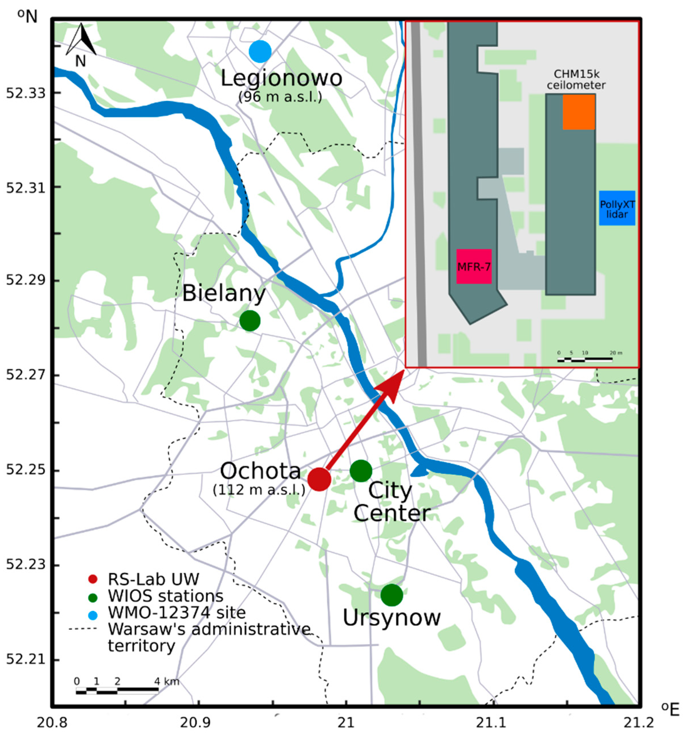
Within this study, two ground-based active remote sensors were utilized: The custom-designed ceilometer (CHM15k model, Lufft/JenOptik, Germany) and the multiwavelength-Raman-polarization lidar PollyXT (collaborative in-house development). Both instruments were operated at the Remote Sensing Laboratory (RS-Lab) of the Institute of Geophysics at the Faculty of Physics of the University of Warsaw, located in Warsaw city center (52.2109°N, 20.9826°E, 112 m a.s.l.). The RS-Lab is equipped with several instruments that were used in this study as auxiliary (locations indicated in Figure 1) or not at all (https://www.igf.fuw.edu.pl/en/instruments/, last access: 11 December 2019). The RS-Lab regularly provides data to several networks: The Polish Aerosol Research Network (PolandAOD-NET, http://www.polandaod.pl, last access: 11 December 2019), the EARLINET (https://www.earlinet.org, last access: 11 December 2019), and the worldwide lidar network Polly-NET (http://polly.rsd.tropos.de, last access: 11 December 2019).

The CHM15k ceilometer was continuously operated in Warsaw from 1 January 2008 to 31 October 2013. It was installed on the roof-platform of the RS-Lab (21 m a.g.l.). The data was acquired with a temporal resolution of 30 s and a spatial resolution of 15 m, with the maximum signal range of 15.36 km (corresponding to 1024 range-bins). The ceilometer comprises a diode-pumped Nd:YAG solid-state laser, which emits low-energy laser pulses (8 µJ), at a high frequency (5–7 kHz), at a wavelength of 1064 nm. The optical design is based on a refracting telescope; the lens has a 100 mm diameter. The lowermost level of the overlap between the emitted laser beam and the receiver lens is at approximately 180 m and the full overlap is completed at approximately 800 m. The CHM15k instrument at the RS-Lab has a custom field of view (FOV, i.e., 0.9 mrad), which results in an optimal overlap and signal-to-noise ratio (SNR) being achieved [29]. For comparison, the standard CHM15k has a narrower FOV (but issues with high overlap) and the CHM15kx has a wider FOV (but issues with background radiation), as discussed in detail by [32]. The automatic manufacturer overlap correction is applied to the ceilometer signals. The standard CHM15k can suffer from the fact that the amplitude of the overlap correction is temperature dependent, this being larger for higher temperatures [56]. The study of the overlap function and the instrumental constant dependence on the internal temperature changes was also done for the RS-Lab CHM15k. From 30 April to 2 May 2012, the ceilometer was installed at the St. Jacob the Apostle Parish located in the small, sparsely populated and spacious rural town of Głowno (51.9645°N, 19.7249°E) in the Central Polish Lowlands. Unique horizontal measurements were taken over the Mrożyczka Reservoir, and thus calculations were done within the range where no local traffic influence was possible. The results showed that for the RS-Lab version of the CHM15k, the temperature effects are negligible. The overlap function was determined from several horizontal measurements to assess the signal quality at ranges near the ceilometer. The closest range-bin for which the signal variability was significant (i.e., >3σ at daytime and >1σ at night) was at the range-bin 12, translating to 180 m. Since November 2013, the ceilometer measurements have been conducted at the SolarAOT Observatory in Strzyzow within the PolandAOD-NET activities. Further details on this particular version of the custom-designed ceilometer are described in [29] and the differences of various versions of the CHM15k and CHM15kx ceilometers are discussed in [32].

The PollyXT lidar was built in a scientific collaboration of the Institute of Geophysics at the Faculty of Physics of the University of Warsaw (IGFUW, Warsaw, Poland) and the Leibniz Institute of Tropospheric Research (TROPOS, Leipzig, Germany). It was installed at the RS-Lab in Warsaw in June 2013. After an extensive test phase, the lidar started operation on 1 July 2013 and has performed quasi-continuous observations ever since. The lidar emits high-energy laser pulses of 180 mJ at 1064 nm, 110 mJ at 532 nm, and 60 mJ at 355 nm, with a repetition rate of 20 Hz. The initial laser beam is expanded to a 45 mm diameter, providing a low beam divergence of 0.2 mrad. The signals are received by two reflecting telescopes: The narrow field of view (1 mrad) large-sized telescope (300 mm diameter) and the wide field of view (2.5 mrad) small-sized telescope (50 mm diameter). The later was installed in April 2016, with the aim of improving the lidar detection range at altitudes close to the ground (<1 km). The measurements are performed at 8-channels, using the large telescope, and at 4-channels, using the small telescope. The 8-channel detection unit (so-called 2α + 3β + 2δ + WV) enables the determination of the extinction coefficient profiles at 532 and 355 nm; the backscatter coefficient at 1064, 532, and 355 nm; the depolarization ratio at 532 and 355 nm; and the water vapor mixing ratio. The 4-channel detection unit (so-called 2α + 2β) is designated for obtaining the extinction and backscatter coefficient profiles at 532 and 355 nm. The signals are recorded up to 48 km (with a pretrigger length of 250 range-bins). The data of all channels is obtained with a standard 7.5 m vertical resolution in temporal steps of 30 s. The overlapping range of the laser beam and the large and the small telescopes is completed at roughly 400 and 120 m, respectively. No overlap correction was applied to the lidar data in this paper. The overlap function of lidar is monitored as the ratio of the signal collected with the small telescope to the signal collected at the large telescope, and thus for two elastic (355 and 532 nm) and two Raman (387 and 607 nm) channels. Additionally, we monitored the stability of the overlap with a camera, the laser pulse energy with a power meter, and the temperature inside the lidar cabinet. The inspection of the monitored parameters shows that typically, the temperature-dependent differences in the overlap are very low (<15 m) and the stability of the lidar signal is high (>98%), which is due to the use of an insulated cabinet equipped with an efficient heating–cooling system. More technical information on PollyXT-type lidars can be found in [57]. The aerosol optical properties retrieval schemes are introduced in [11,58,59]. The aerosol microphysical properties’ retrieval is described in [60] and the water vapor derivation methodology in [61].

Concerning the overlap region of the two sensors, the lowest possible height of ABLH that can be unambiguously detected with the ceilometer and lidar (large telescope) is at 195 m a.g.l. Note that the lidar range resolution is reduced to merge the ceilometer range resolution of 15 m, whereby the lidar initial range-bins 4th and 5th correspond to the ceilometer 1st range-bin.

Note that for both instruments described here, the signal-to-noise ratio depends on the solar background illumination and the presence of molecules and particles suspended in the atmosphere, whereby it decreases rapidly when the optical depth of the atmosphere declines. The SNR was calculated using the approach described in [62].

The auxiliary instrumentation of the RS-Lab that was used in this paper comprises the sensors installed at two roof platforms (Figure 1), i.e., the weather transmitter WXT510 (Vaisala), the disdrometer OTT (Parsivel), the passive multi-filter rotating shadowband radiometer on a solar tracker MFR-7 (Yankee Environmental Systems), and the sun photometer CE318 (CIMEL Electronique); the latter has been operated since 1 January 2018.

3. Methodology

3.1. Atmospheric Boundary Layer Heights from Lidar and Ceilometer

As already described in the introduction, several studies have demonstrated that the PollyXT lidars and CHM15k ceilometers are reliable in detecting atmospheric aerosol structure and evolution. The first automated ABLH retrieval for one year of the PollyXT lidar data was reported by [25]. The annual ABLH cycles derived from 4-year CHM15k ceilometer observations were reported by [29]. In the current paper, the ABLH datasets derived from these two instruments were obtained using an automated routine and utilized to derive the decadal coverage of the ABLH variability over Warsaw.

The auxiliary instrumentation was used for identifying the fog/smog and precipitation, as well as for distinguishing clear-sky from cloudy days.

The fog/smog and precipitation conditions were identified using of the following information: The RS-Lab roof platform measurements of the metrological data with the WXT510 (Vaisala) weather transmitter and the OTT disdrometer, the aerosol optical depth (AOD) derived from the MFR-7 and CE318 sun photometer, as well as the particulate matter, PM_2.5 and PM₁₀, concentrations measured by the air quality monitoring WIOS stations (Figure 1). The WIOS data are publicly available via the Archive of the Chief Inspectorate for Environmental Protection of Poland (http://powietrze.gios.gov.pl/pjp/archives, last access: 11 December 2019).

The clearness index of the sky can be quantified with the use of the instantaneous extraterrestrial solar fluxes reaching Earth’s surface [63], which are a good indicator for distinguishing clear from cloudy days at daytime. At the RS-Lab roof platform, the MFR-7 radiometer measures the global and diffuse fluxes and the pyranometer the hemispheric solar radiation flux density. The fluxes are obtained only in daytime, and thus another method is needed to estimate the sky clearness at nighttime. Therefore, for both day and night observations, the state-of-the-art cloud screening procedure of EARLINET is applied [64]. This procedure is used by the so-called Single Calculus Chain (SCC) software developments (https://scc-documentation.readthedocs.io, last access: 16 December 2019). Note that in this paper, the clear-sky definition includes the cloudless scenarios, as well as the scenarios for which Cirrus clouds occur above 8 km over the measurement site.

The specific aim was to derive the diurnal cycles of the ABLH, defined as starting at night, with the nocturnal boundary layer (NL), characterized by stable air with sporadic turbulence, followed (after sunrise) by a development of the well-mixed layer (WML) during the day, and after sunset, the residual layer (RL) in place of the mixed layer, and/or the stable boundary layer near the ground [1,2,3]. The boundary layer heights derived from the lidar and ceilometer data are related to the aerosol load present in the lowermost atmosphere, and therefore they do not precisely correspond to the atmospheric boundary layer height as defined therein. In comparison with the idealized definitions, the lidar and ceilometer ABLHs are derived based on an apparent aerosol load change, which occurs between the atmospheric boundary layer and the free troposphere. However, even if this relation is not simple, in this paper, it was assumed that they are proportional. The ABLH derived around sunrise and sunset was defined as the transition layer (TL). As the WML, TL, RL, and NL are related to certain times of the day, which depends on the season; their definitions are given in

Table 1. The definitions of the time duration for the boundary layer per season used in this study. The given times were assessed as corresponding to the listed periods in different seasons and do not represent the mean values. Times are given in UTC.

	Spring (MAM) Autumn (SON)	Summer (JJA)	Winter (DJF)
Daytime	05:00–17:00	04:00–19:00	06:00–15:00
Nighttime	19:00–04:00	20:00–03:00	16:00–06:00
Well-mixed layer (WML)	12:00–16:00	12:00–17:00	12:00–14:00
Transition layer (TL) sunrise	05:00–11:00	03:00–11:00	06:00–11:00
Transition layer (TL) sunset	17:00–19:00	16:00–20:00	15:00–16:00
Nocturnal and residual layer (NL, RL)	20:00–04:00	21:00–02:00	17:00–05:00

.

From the individual diurnal cycle data, the monthly mean diurnal cycles and the annual cycles of the ABLH, the seasonal mean ABLHs, and the annual mean NL, WML, and RL heights, as well as the daytime and nighttime ABLH frequency distribution, were derived. The time duration of daytime and nighttime per season used in this study are specified in Table 1. For comparison, the exact sunrise and sunset times are available via https://www.timeanddate.com/sun/poland/warsaw. Warsaw is located in the Central European Summer Time zone, i.e., CEST = UTC/GMT + 2 h. The daylight-saving time starts on 31 March with 1 hour forward and ends on 27 October with 1 hour back. The local time is divided to LT = UTC + 2 h (so-called local summertime) or, LT = UTC + 1 h (so-called local wintertime).

More information can be found at https://www.timeanddate.com/worldclock/poland/warsaw (last access: 11 December 2019). Note that all analyses were performed in local time, but in this paper, the values are given in UTC.

The elastically backscattered 1064 nm lidar and ceilometer signals were used for the boundary layer detection. The range resolution of the two instruments was merged to ceilometer resolution (15 m). Thus, the re-binning was applied before the data processing. The 4th and 5th range-bins of the lidar (block average) corresponding to 33.75 m a.g.l. was merged to the 1st range-bin of the ceilometer (on the roof platform) corresponding to 36 m a.g.l. The resulting difference was regarded as negligible.

The lidar and ceilometer signals were collected with a 30 s resolution but the ABLH detection was performed on the 10 min averaged range-corrected backscatter signals. Then, the sliding average in time was applied, thus one 10 min average signal was provided every 30 s. Three different algorithms were used on these signals to estimate the ABLH. In the gradient method (hereafter GDT), the first derivative of the signal logarithm (with height) is used and the strongest negative gradient marks the ABLH. The second method is based on investigating a standard deviation of the signals (hereafter STD). The standard deviation of the averaged signals (after the sliding average) is calculated over the 10 min window, and then the altitude at which the standard deviation is maximal marks the ABLH. The wavelet covariance transform method (hereafter WCT) comprises analysis of the vertical signal gradient and fast temporal changes in the signal time series, as a function of the height. On the one hand, the advantage of the WCT method is that it is less affected by the signal-to-noise ratio than the two other methods [25,41]. On the other hand, the main challenge of this method is to find an appropriate value of the dilation, a. In this paper, the dilation defined as 4 times the range resolution of 15 m was used, based on a sensitivity study conducted to optimize the choice of dilation. Smaller dilation values resulted in numerous local minima and prevented unambiguous detection of ABLH. Thus, the height window of 60 m was used for the time window of 10 min (for both instruments).

In order to reduce the impact of the overlap-affected range of the remote sensing measurements [65] and the middle-level clouds [53], the lower and the upper limit for the derived ABLH was defined. Within the blind region of the incomplete overlap range of each instrument, the received signal is extremely weak and dominated by noise, thus it is difficult to obtain a valid ABLH, except for particular conditions, such as very low clouds, fog, or smog (even then, the accuracy of the retrieval is low). Above the blind region, when the laser beam begins to enter the telescope’s field of view, the signal increases and the SNR improves. In the range of the completed overlap, the SNR is entirely driven by the scattering and absorption by molecules and particles suspended in the atmosphere. Thus, both instruments need a defined lowest level height (concerning the blind region of the incomplete overlap) to maintain high-quality calculations [62].

The cloud bottom heights (CBHs) derived within the 3-km altitude were regarded as marking the top of the boundary layer. The CBH was detected by the strongest positive change in the range-corrected backscatter signal of the lidar or ceilometer measurement. Generally, clouds influence short-wave and long-wave radiation, as well as latent and sensible heat flux, thus consequently, the boundary layer diurnal cycle. They can form either at the top of the daytime mixed boundary layer or at the base of the stable (usually nocturnal) boundary layer. Their occurrence is closely connected to thermodynamics within the boundary layer. Low-level clouds (cloud bottom heights < 2 km) are a frequent phenomenon in the boundary layer, especially cumulus and stratocumulus that often occur at the top of the boundary layer (a so-called boundary layer cloud). Therefore, the upper limit of the ABLH retrieval was set to 3 km. This is in accordance with the mixing layer heights reported for other continental sites as being below this altitude [17,25,26,29,66,67,68]. Note that, in general a ceilometer signal is less powerful compared to that of lidar, and therefore the excellent ability of ceilometers to detect aerosols is practically limited up to approximately a 3 km height [62,65,69]. For the cases when the algorithm chooses the cloud as the top of ABL, when such a cloud is at the altitude of 3 to 6 km (i.e., middle-level clouds), it is not used as marking the ABLH, as it is considered to be detached from the boundary layer [1,2,3].

3.2. Atmospheric Boundary Layer Heights from Rawinsondes

Balloon soundings are frequently done with the use of radiosondes that measure atmospheric pressure, temperature, and humidity. When the radiosonde position is tracked to also provide the wind speed and direction it is called a rawinsonde. Rawinsondes launches at the World Meteorological Organization site closest to Warsaw were used. The WMO-12374 site in a small town Legionowo (52.40°N, 20.96°E, 96 m a.s.l.) is located 25 km north of the RS-Lab. Note that Warsaw and Legionowo are characterized by a flat orography, with a maximum elevation difference below 40 m a.g.l. between the two measurement sites (an elevation map of the 50 km² area is available at https://en-us.topographic-map.com/maps/tlmm/Warsaw, last access: 11 December 2019).

The RS92 rawinsondes (Vaisala, Finland) are launched twice a day at 00:00 and 12:00 UTC. They provide vertical profiles of, amongst others, the atmospheric pressure, temperature, dew point temperature, relative humidity, and wind speed. These parameters were used in our study for different retrievals. The ABLH was identified in the rawinsonde profiles using two methods. The first one was based on identifying the height of a sharp change in the temperature (or dew point temperature) and the relative humidity profiles on the skew-T-log-p diagram used frequently for radiosondes [70]. The second one was the bulk Richardson (bulk-Ri) method [71], which is known to be favorable for ABLH retrieval in both stable and convective conditions [51], whereby this method requires rawinsondes. The bulk-Ri method uses the ratio of the turbulence associated with buoyancy to that associated with mechanical shear, and the ABLH is defined as the lowest height at which Ri matches the critical value of 0.25 [71].

Rawinsondes’ data were obtained from the Upper Air Data website of the University of Wyoming (http://weather.uwyo.edu/upperair/sounding.html, last access: 11 December 2019).

The diagrams of rawinsondes for the discussed measurement period of 2008 to 2018 are depicted as quick-looks at the PolandAOD-NET Website (http://www.Polandaod.pl, last access: 16 December 2019).

4. Results of Boundary Layer Height Retrieval Comparison

The ABLH values derived from lidar and ceilometer signals were compared against the ABLHs derived independently from the rawinsondes meteorological profiles. The direct lidar–ceilometer comparison was performed as well. This analysis was done for the 4 months when the ceilometer and lidar performed simultaneous observations from 1 July to 31 October 2013. The observations conducted under clear-sky and cloudy weather were analyzed while those collected in fog/smog and precipitation were not used.

4.1. ABLH Comparisons for Lidar, Ceilometer, and Rawinsondes Data

Within the time window of 1 July to 31 October 2013, all lidar and ceilometer measurements in Warsaw that were coincident with the rawinsondes’ launches at 00:00 and 12:00 UTC in Legionowo were compared. Due to the limited availability of the coincident data (mainly due to lidar), only 84 profiles were available for comparison. As for the rawinsonde evaluated with the skew-T-log-p method, five profiles with no significant inversion in the temperature or the dew point temperature profile were screened. The inversion threshold was defined as the difference in the value of the two adjacent temperature points exhibiting a sharp gradient of at least 3 °C. Lidar and ceilometer profiles for which the ABLH was >3 km in altitude (three cases) were screened [70,72]. The data points where the ABLHs difference between the rawinsonde lidar or rawinsonde ceilometer was >2 km (four cases) were screened, as in those cases each instrument clearly measured a different air mass [60,61,69].

The ABLHs derived from active remote sensors using the GDT, STD, and WCT methods, separated to clear-sky and cloudy conditions, for both pairs of instruments (lidar rawinsonde and ceilometer rawinsonde) are shown in corresponding scatter plots in Figure 2 (for brevity, only results for the bulk-Ri method are shown). For all plots, a linear fit to 72 data points was made. In general, the fitted lines indicate a better correspondence of ceilometer than lidar to the rawinsonde. Note that the Pearson correlation coefficients in this paper were calculated to assess the linear relationship between the two variables (ABLH values) derived with the different methods. When the significance level was p ≤ 0.05, then the correlation coefficient was considered statistically significant. All correlations reported in this paper were found to be statistically significant, unless explicitly stated otherwise. The correlation coefficients are denoted as R² and the corresponding standard deviation as SD.

In

Table 2. The correlation coefficient (R²) and the standard deviation (SD) of the ABLHs derived from lidar and ceilometer by using the GDT, STD, and WCT methods versus the ABLHs derived from rawinsonde by using the skew-T-log-p and the bulk-Ri methods. Results obtained during clear-sky and cloudy conditions from July to October 2013.

July to October 2013	Lidar			Ceilometer
	GDT	STD	WCT	GDT	STD	WCT
Bulk Richardson method
All measurements	R2 = 0.69	R2 = 0.68	R2 = 0.70	R2 = 0.78	R2 = 0.70	R2 = 0.80
N = 72	SD = 0.50 km	SD = 0.51 km	SD = 0.48 km	SD = 0.38 km	SD = 0.43 km	SD = 0.36 km
Clear-sky conditions	R2 = 0.70	R2 = 0.72	R2 = 0.74	R2 = 0.88	R2 = 0.78	R2 = 0.90
N = 34	SD = 0.61 km	SD = 0.46 km	SD = 0.42 km	SD = 0.30 km	SD = 0.45 km	SD = 0.29 km
Cloudy conditions	R2 = 0.66	R2 = 0.55	R2 = 0.60	R2 = 0.73	R2 = 0.59	R2 = 0.75
N = 38	SD = 0.56 km	SD = 0.53 km	SD = 0.54 km	SD = 0.47 km	SD = 0.53 km	SD = 0.43 km
Skew-T-log-p method
All measurements	R2 = 0.62	R2 = 0.59	R2 = 0.63	R2 = 0.75	R2 = 0.64	R2 = 0.76
N = 72	SD = 0.60 km	SD = 0.61 km	SD = 0.59 km	SD = 0.44 km	SD = 0.52 km	SD = 0.43 km
Clear-sky conditions	R2 = 0.64	R2 = 0.61	R2 = 0.65	R2 = 0.82	R2 = 0.72	R2 = 0.83
N = 34	SD = 0.55 km	SD = 0.57 km	SD = 0.53 km	SD = 0.36 km	SD = 0.48 km	SD = 0.36 km
Cloudy conditions	R2 = 0.62	R2 = 0.52	R2 = 0.56	R2 = 0.64	R2 = 0.49	R2 = 0.68
N = 38	SD = 0.62 km	SD = 0.58 km	SD = 0.62 km	SD = 0.49 km	SD = 0.55 km	SD = 0.47 km

, the results regarding the lidar and ceilometer ABLHs comparisons with the two rawinsonde retrieval methods are listed. In Figure 3, the correlation plot of ABLHs calculated using the skew-T-log-p method versus the bulk-Ri method for daytime and nighttime rawinsonde launches are plotted.

The scatter plot of the lidar-rawinsondes ABLHs is given in Figure 2, top row. Regardless of the applied retrieval method, the correlation coefficients were found to be positive and relatively high, although accompanied by a significant standard deviation. The differences in the correlation coefficients were negligible within the obtained range of the standard deviations. The best agreement of the lidar-derived ABLHs was obtained for the WCT method (R² of 0.70 and SD of 480 m), then for the GDT method (0.69 and 500 m), and the STD method (0.68 and 510 m), when compared to the rawinsonde.

The comparison results for the ceilometer-rawinsonde ABLHs are given in Figure 2, bottom row. The positive correlation coefficients obtained for ceilometer versus rawinsonde were somewhat higher than those derived for lidar versus rawinsondes, being the highest for the WCT (R² of 0.80 with SD of 360 m), then the GDT method (0.78 and 380 m), and the STD method (0.71 and 430 m). An underestimation of the ceilometer ABLHs (regardless of the derivation method and altitude range), concerning the rawinsonde ABLHs, was clearly discernible.

The ABLHs shown in Figure 3 for direct comparison of the skew-T-log-p method and the bulk-Ri method have an R² of 0.9 and SD of 0.32 km. Note that the daytime and nighttime rawinsondes are plotted separately. For many data points, the skew-T-log-p method retrievals are overestimated, which (as expected) favors the bulk-Ri method, as the latter considers both buoyancy-produced and mechanically produced turbulence [51]. One can see that in the samples of daytime (related to WML; N = 39) and nighttime (NL, N = 33) measurements over Legionowo, there are some ABLH values derived within the range 1.5–2.5 km at nighttime. This gives confidence that a few such high ABLH values obtained for NL from lidar/ceilometer are not an artifact.

Advected residual or lofted aerosol can sometimes be observed at nighttime in Warsaw and its vicinity, and it can lead to ABLH > 2 km. This agrees with observations under heat wave conditions reported in [11], where semi-persistent growth of ABLH values to extreme levels is discussed as being due to an injection of long-range transported pollution from Germany into the urban boundary layer over Warsaw. Several high ABLHs at nighttime are also reported for statistical analyses of the boundary layer optical properties by [52], where one of the possible reasons discussed is aerosol bursts [73]. As shown in Figure 3, ABLHs derived in Legionowo confirm the possible existence of such high NL in the vicinity of Warsaw city. Therefore, the values are in relation to the true boundary layer top variability.

Comparison studies for the collocated rawinsonde-lidar ABLHs revealed high correlation coefficients of 0.91 for stable and 0.96 for unstable environments [21]. For the collocated rawinsonde-ceilometer AHLHs, the correlation coefficients of 0.9 in convective conditions and 0.8 for stable conditions were reported [34]. The ABLH correlation coefficients of 0.85, 0.82, and 0.89 were reported for using, respectively, the gradient method, cluster method, and wavelet method applied to ceilometer data, as compared to rawinsonde-derived ABLHs [70]. Therefore, this kind of comparison was regarded as an appropriate approach to verify the accuracy of the ABLHs derived from the lidar and ceilometer. However, in the current study, the difference in the location of the rawinsonde and the location of the lidar and ceilometer resulted in somewhat lower correlation coefficients concerning the values reported in the literature. The low number of samples and the method applied for rawinsonde ABLH retrievals can play a role in such a comparative study [17,44]. This cannot be excluded also in our case, which is visible in Table 2, whereby the performance of one of the methods is indeed better.

The lidar-rawinsonde and ceilometer-rawinsonde ABLHs for clear-sky and cloudy conditions for the period from July to October 2013 are listed in Table 2. For both lidar and ceilometer, the best results in terms of the highest correlation coefficient and the lowest standard deviation were obtained in clear-sky conditions (WCT method) and the worst in cloudy conditions (STD method). Comparisons of the rawinsonde bulk-Ri method retrievals with the lidar/ceilometer GDT, STD, and WCT retrievals shows that (regardless of the weather conditions) the standard deviation is higher for the rawinsonde versus lidar (420–540 m) than for the rawinsonde versus ceilometer (290–430 m), whereby the highest standard deviations were obtained for the STD method.

The correlation coefficients were in the range 0.55–0.74 for the lidar rawinsonde and 0.59–0.90 for the ceilometer rawinsonde. As for comparisons of the skew-T-log-p with the lidar/ceilometer retrievals, they show consistent results with the bulk-Ri comparisons, with somewhat lower R² and SD. Based on the values given in Table 2, the WCT method performed the best, except for one case (the GDT for lidar in cloudy conditions). As for the analyses of the differences between the clear days and the cloudy days shown in Table 2, it must be mentioned that although they are present, they are not statistically significant.

The discrepancies found between the ABLHs derived from the three different instruments must be at least partly attributed to the differences in the measurement technique (the active remote sensing versus the in-situ sounding) as well as to the retrieval algorithms and their physical definition (the tracking of sharp changes in the aerosol load versus the marking of the top of the mixing process, with respect to the thermodynamic principle). The differences are expected also due to the atmospheric conditions, so when complex aerosol layers or boundary layer clouds appear within 3 km, different results between the rawinsonde and lidar/ceilometer ABLH retrieval can be expected [21,70]. Therefore, the higher correlation coefficients are expected to be obtained for the typical clear-sky-biased analyses [34,37,39]. Thus, in the case of occurrence of very local phenomena, such as fog or smog at one of the sites, data points should not be used for comparative analyses. The differences attributed to the distance (25 km), the elevation altitudes (112 versus 96 m a.s.l., and the near-surface conditions (city center versus semi-rural) at the two sites can be considered, especially in the lowermost atmosphere. The elevation altitude differences mentioned here are not related to retrieval uncertainties but the physical features in the atmosphere above each measurement site.

The impact of the distance, local surroundings, and the near-surface conditions was reported as not significant for the relative humidity profiles’ comparison at the two sites in Warsaw and Legionowo [61]. For these cities, more of a concern was the large-scale circulation [11,59] and the air-mass inflow with a related height-dependent tropospheric wind direction change at each site [60,61]. Therefore, for certain meteorological conditions, higher correlations can be expected, e.g., for the air-mass transport within less than 1 h along the north–south transect between the two cities [60].

The comparison study of the mixing height (calculated using the gradient method combined with the wind speed threshold method) between Wien Hohe Warte (suburban) and Obersiebenbrunn (rural) located at a distance of roughly 30 km, with an elevation difference of above 70 m between the two sites, revealed that local conditions could give rise to occasional large differences in the mixing height [74]. The frequency distribution analysis of the ABLH differences among Pairs (urban metropolitan), Palaiseau (suburban), and Trainou (rural), located at a distance of 20 km from each other, with even more significant differences in elevation (28 m to 159 m), revealed the urban ABLH was higher than the rural ABLH during daytime and higher that of the suburban during nighttime [75]. In our case, no clear conclusion was drawn on the ABLH difference between the two sites in Warsaw and Legionowo, as related to urban versus rural effects.

4.2. Comparison of ABLH Derived by Lidar and Ceilometer under Different Conditions

Further comparison of the ABLHs derived from lidar and ceilometer measurements under certain conditions, i.e., day versus nighttime and clear-sky versus boundary layer clouds, were performed. The results of these direct comparisons obtained with the three methods (GDT, STD, and WCT) showed consistent results, and therefore, only the results of WCT method comparison are shown in Figure 4 for brevity.

The WCT method was found to have the highest correlation coefficient with the lowest standard deviation for all conditions. Only for the cloudy conditions did the GDT method (not shown) perform slightly better. In Figure 4, top, the comparison in daytime conditions (999 data points) indicated a higher performance (R² of 0.95 and SD of 180 m) than that for the nighttime conditions (823 data points, 0.91 and 220 m, respectively). In Figure 4, bottom, the comparison of the clear-sky conditions (defined as lacking any clouds except Cirrus; 972 data points) showed a better performance, with an R² of 0.95 and SD of 190 m, than the cloudy conditions (boundary layer low clouds; 812 data points, 0.91 and 200 m, respectively).

Note that the comparisons of the rawinsondes-lidar and the rawinsondes-ceilometer ABLHs shown in Figure 2 and listed in Table 2 had significantly higher standard deviations (two to three times) and lower correlation coefficients than the direct comparisons of the lidar-ceilometer ABLHs shown in Figure 4.

5. Scaling Threshold-Based Method for Consistent Lidar and Ceilometer ABLH Retrieval

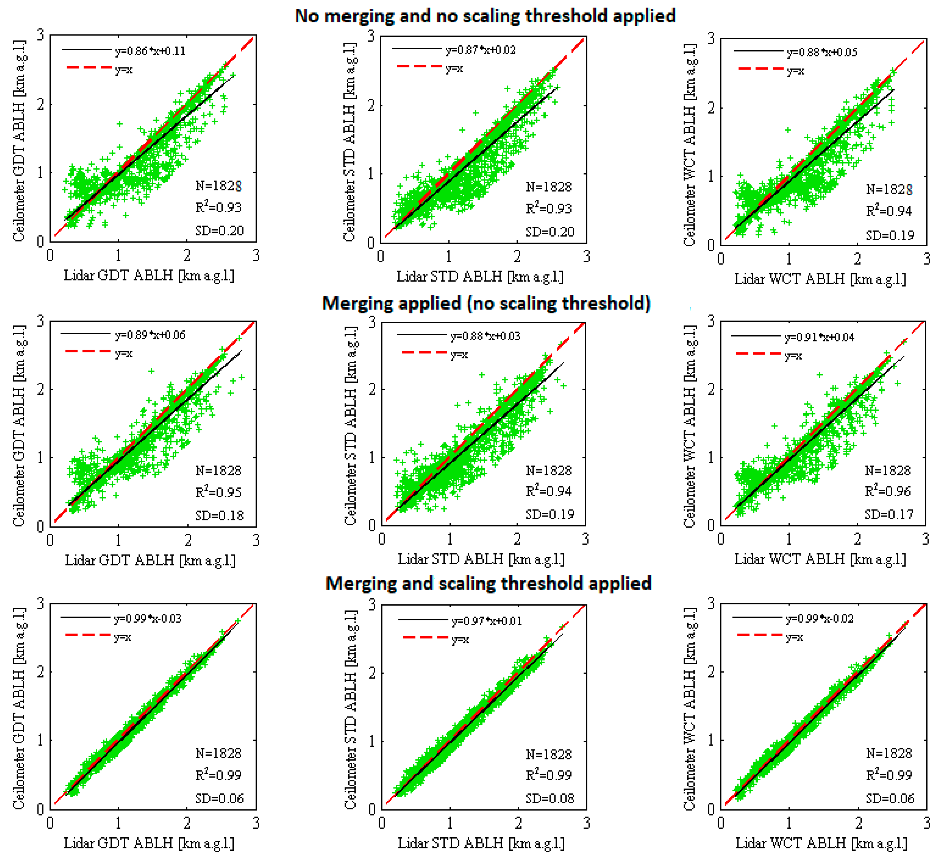
The direct comparison of the ABLHs derived from the collocated lidar and ceilometer measurements using the three methods (GDT, STD, and WCT) is shown in Figure 5. From July to October 2013, the data sample of 1828 measurements (each data point represents the 10 min average) was compared. In Figure 5, top subfigures, the lidar and ceilometer data are not merged (i.e., they were obtained for initial resolutions of 7.5 m for lidar and 15 m for ceilometer, and the difference in each instrument elevation height was not considered). The correlation coefficients obtained for each of the three methods are high (0.93 < R² < 0.94) with the standard deviation in a range that corresponds to the initial bias (300 m) of the lidar-ceilometer measurements (0.19 < SD < 0.2 km). Generally, below the altitude of 0.7 km, the lidar-derived ABLHs are slightly lower in comparison to the ceilometer-derived values while above the altitude of 1 km, the opposite tendency is observed (this is also evident in Figure 4). In Figure 5, middle subfigures, one can see that lidar-to-ceilometer signal re-binning and merging (as in Section 3.1) slightly improved the data correlation (0.94 < R² < 0.96) and decreased the standard deviation (0.17–0.19 km), resulting in reduced bias (200 m).

In order to further reduce the bias in the lidar-ceilometer ABLH retrievals, the threshold-based scaling method was developed and applied to the merged data. In this paper, the choice to scale the lidar-to-ceilometer ABLHs was made for two reasons. Firstly, there are much more low-power ceilometers over Europe than complex high-power lidars, and therefore the ceilometers can be regarded as reference instruments for ABLH retrieval. Secondly, it was considered that the results of the comparisons of the lidar-rawindsonde and the ceilometer-rawindsonde ABLH values (discussed in Section 4.1) showed more consistent results for the latter.

The working principle of the threshold-based scaling algorithm is given below.

Let us denote SD as the standard deviation obtained for the direct comparison of the ceilometer-derived ABLH (denoted CH) and the merged lidar-derived ABLH (denoted LH) collected during the collocated side-by-side measurements. Then, the scaled LH_new can be obtained as in Equations (1) and (2):

$$L{H}_{new} = \{\begin{array}{c}LH,0\le Y1<2SD\\ LH-1.5SD,2SD\le Y1<3SD\\ LH-2.5SD,3SD\le Y1<4SD\\ LH-3.5SD,Y1\ge 4SD\end{array},$$

(1)

where Y1 = (LH − CH).

$$L{H}_{new} = \{\begin{array}{c}LH,0\le Y2<2SD\\ LH+1.5SD,2SD\le Y2<3SD\\ LH+2.5SD,3SD\le Y2<4SD\\ LH+3.5SD,Y2\ge 4SD\end{array},$$

(2)

where Y2 = (CH − LH).

The scaling Equations (1) and (2) are not directly based on any physical process. Still, indirectly, they have a physical basis, which is exposed in the standard deviation of the initially derived ABLHs. Two instruments are available, each sensing the atmosphere with the identical principle but using a different technological solution for the light source and the detection system.

Hence, discrepancies can be expected in the derived ABLH, which are due to differences in the initial sensitivity to atmospheric aerosol and molecules sensed by the ceilometer and/or the lidar (due to the different signal intensities). Consequently, the proposed scaling method assumes that those differences are visible in the standard deviation. Note that this approach cannot be treated as the data correcting procedure but instead as the scaling approach to homogenize the datasets obtained by the two instruments. Also, this has nothing to do with any judgment of which instrument is better or worse.

In Figure 6, bottom subfigures, the improvement of the comparison results due to an application of the proposed scaling scheme is depicted by lowering the bias significantly, i.e., to only 60 m for the GDT and WCT methods, and only slightly higher at 80 m for the STD method. The correlation coefficients are very high (0.99) for all the tested ABLH retrieval methods.

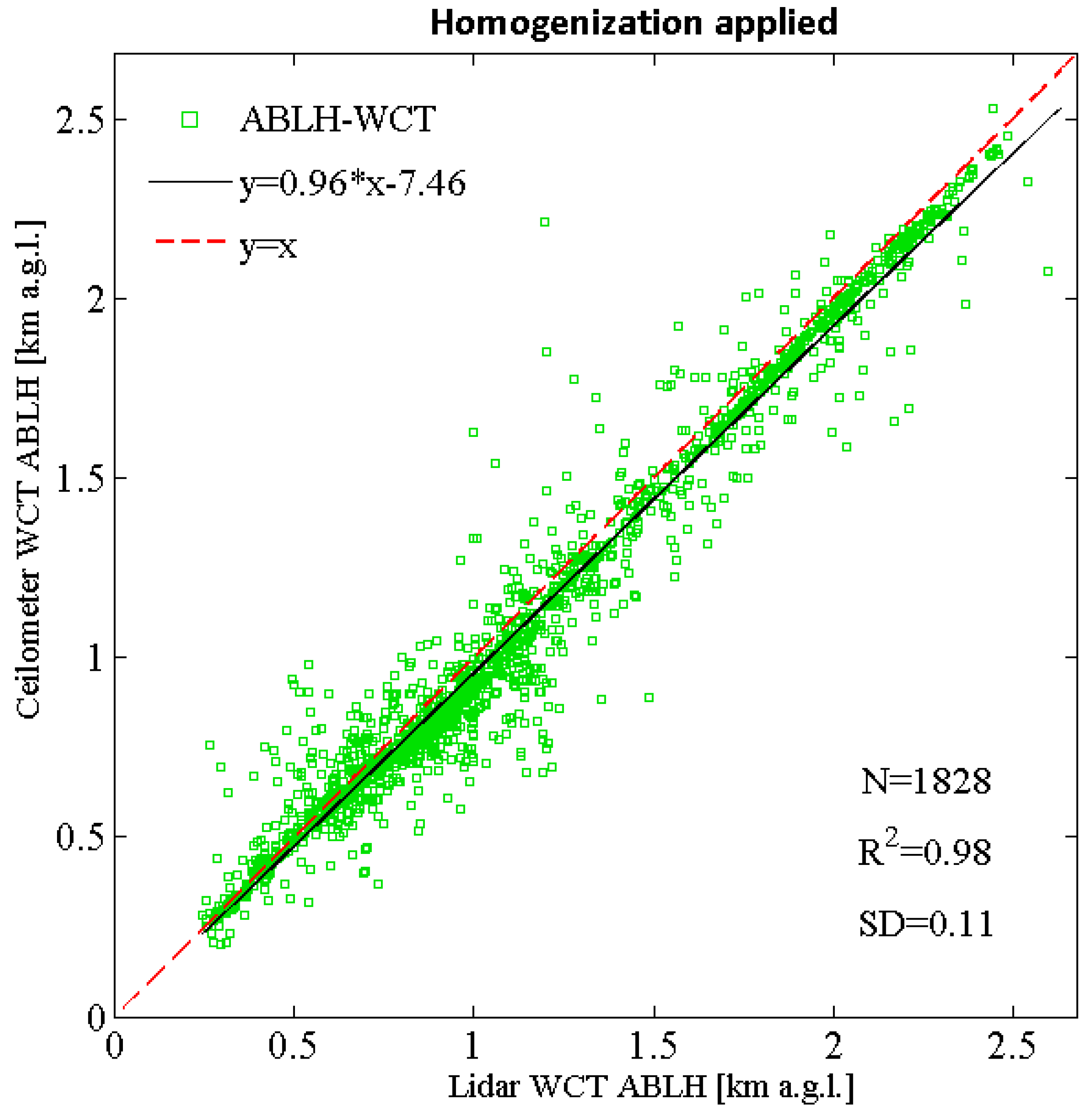
Note that the Equations (1) and (2) can be applied only for the days when the collocated lidar and ceilometer measurements are available. However, from 1 November 2013, the measurements in Warsaw were conducted only with the PollyXT lidar. When only lidar measurements are available, the calculation of the standard deviation of lidar-ceilometer ABLHs is not possible, and hence, the universal method is needed to solve this issue. As a solution, the standard deviation of the lidar-derived ABLH was examined to provide a possible indication on the inadequacies of the retrieval. The standard deviation of the lidar-derived ABLHs (denoted SD_L) was obtained within every 10 min average and used as an independent threshold. Then, the lidar-derived ABLH (denoted LH) was scaled to the new value (LH_new) to homogenize the datasets, as given in Equation (3):

$$L{H}_{new} =\{\begin{array}{c}LH,LH\le 0.7 \mathrm{km}\wedge S{D}_L<0.10 \mathrm{km}\\ LH+1.5S{D}_L,LH\le 0.7 \mathrm{km}\wedge S{D}_L>0.10 \mathrm{km}\\ \\ LH,0.7 \mathrm{km}<LH\le 1.5 \mathrm{km}\wedge S{D}_L<0.15 \mathrm{km}\\ LH-1.5S{D}_L,0.7 \mathrm{km}<LH\le 1.5 \mathrm{km}\wedge S{D}_L>0.15 \mathrm{km}\\ \\ LH,1.5 \mathrm{km}<LH\le 3.0 \mathrm{km}\wedge S{D}_L<0.20 \mathrm{km}\\ LH-3.5S{D}_L,1.5 \mathrm{km}<LH\le 3.0 \mathrm{km}\wedge S{D}_L>0.20 \mathrm{km}\end{array}$$

(3)

In Figure 6, the ceilometer-derived ABLHs are used to test the lidar-derived ABLHs obtained by applying the homogenization algorithm as in Equation (3). The resulting correlation coefficient of the two instruments is an R² of 0.98, and an SD of 0.11 km was obtained. Similarly, high numbers were also obtained for the clear-sky versus cloudy conditions and the daytime (well mixed) versus nighttime (stable) (not shown for brevity). This demonstrates that the proposed method is reliable and can provide coherent results for both datasets. Therefore, it was applied to all lidar-derived ABLHs from 1 November 2013 to 31 December 2018.

Overall, the correlation of ABLHs obtained from the lidar and ceilometer measurements (Figure 4 and Figure 5) are high (R² > 0.91, with SD < 0.22 km) for all performed comparison tests. Therefore, after applying the homogenization, a good continuity of the observations is expected during the whole period of interest (2008–2018). The WCT method applied on the merged signals for the scaled datasets (Figure 5, bottom subfigures, and Figure 6) was identified as the best option for conducting further analyses of the decadal datasets, combining the lidar and ceilometer observations in Warsaw.

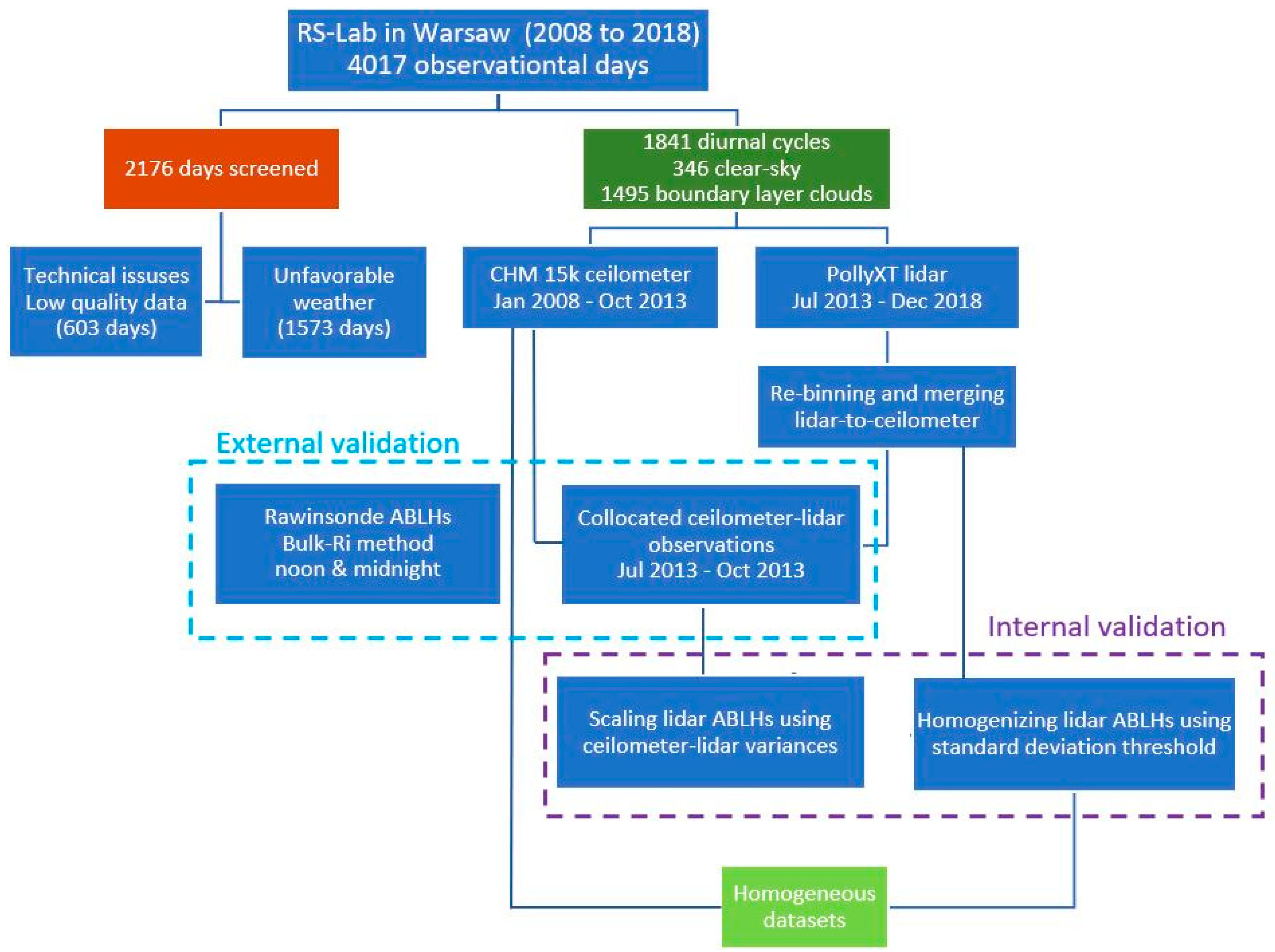
The homogenization algorithm workflow is given in Figure 7.

6. Statistical Analyses of a Decade of ABLH Measurements in Warsaw

A decade of long-term observations of CHM15k ceilometer and PollyXT lidar performed in Warsaw from 2008 to 2018 were used for the statistical analyses. The ceilometer measurements from 1 January 2008 to 31 October 2013 and the lidar measurements from 1 November 2013 until 31 December 2018 were homogenized and combined.

A total number of 1841 daily evolution measurements were obtained, whereby the valid observation day was defined as providing data for at least 12 h on that day (with a minimum of 6 h per day and per night). The observation day was regarded as a clear sky if no cloud occurred within at least 12 h (except Cirrus > 8 km). The separation methodology for the clear-sky and the cloudy days is detailed in Section 4.

For further analyses, the following are defined as providing representative values:

The diurnal cycle: More than 12 h/day of measurements, with a minimum of 6 h per day and per night;

The annual cycle: More than six monthly mean values per year; and

The monthly mean: At least 3 days, each with more than 12 h/day of measurements, with a minimum of 6 h per day and per night;

The seasonal mean: At least 10 days, each with more than 12 h/day of measurements, with a minimum of 6 h per day and per night, within the 3-month-long season in each year; and

The yearly mean: At least 3 days, each with more than 12 h/day of measurements, with a minimum of 6 h per day and per night, for at least 8 months in each year.

Within the subset of the 1841 daily evolution observations, the daytime/nighttime and the cloudy/clear-sky coverage do not significantly influence the data sample. There is no bias towards any of those conditions due to the well-defined subsample focused on capturing the diurnal cycle.

The number of valid observational days for each year under the analyses is listed in

Table 3. The number of lidar/ceilometer-derived diurnal cycles of the atmospheric boundary layer over Warsaw, for the years 2008 to 2018. The number of the available clear-sky cycles is given in brackets. The percentage of clear-sky data to the total number of observations is indicated for each year and each month. Note that before 31 October 2013, the ceilometer data were used, and after that date, the lidar data were used (denoted with *).

	Jan	Feb	Mar	Apr	May	Jun	Jul	Aug	Sep	Oct	Nov	Dec	Total	%
2008	8(1)	8(0)	10(1)	8(2)	9(2)	7(3)	4(2)	9(3)	9(1)	12(2)	9(2)	31(6)	124(25)	20
2009	29(7)	6(0)	15(2)	18(11)	8(1)	17(0)	18(0)	9(3)	5(1)	10(1)	9(2)	7(0)	151(28)	19
2010	15(4)	7(0)	21(2)	20(3)	28(0)	24(5)	28(9)	14(1)	7(1)	16(8)	9(1)	6(2)	195(36)	18
2011	7(0)	13(5)	31(9)	30(7)	29(4)	29(3)	24(2)	9(1)	30(7)	31(8)	30(8)	31(0)	294(54)	18
2012	31(4)	29(5)	31(7)	27(3)	23(4)	21(0)	10(4)	16(1)	16(3)	0	0	11(0)	215(31)	14
2013	31(1)	28(0)	31(9)	30(3)	31(3)	30(3)	31(4)	31(5)	30(4)	18(3)	* 9(0)	0	300(35)	12
2014	0	0	0	4(1)	12(2)	7(1)	12(2)	13(0)	0	0	0	2(0)	50(6)	12
2015	0	0	12(4)	7(2)	0	0	8(0)	20(19)	2(1)	0	0	5(0)	53(26)	49
2016	0	5(0)	10(0)	6(0)	8(0)	21(3)	22(1)	28(6)	24(13)	10(0)	3(2)	11(1)	148(26)	18
2017	15(2)	0	3(0)	0	12(3)	29(3)	20(1)	6(0)	17(2)	21(3)	0	0	123(14)	12
2018	0	18(3)	17(4)	23(6)	12(7)	21(6)	14(6)	19(9)	11(6)	23(10)	20(6)	10(2)	188(65)	35
Total	136(19)	114(13)	181(38)	173(38)	172(26)	206(27)	191(31)	174(48)	151(39)	141(35)	89(21)	113(11)	1841(346)	19
%	14	11	21	22	15	13	16	28	26	25	24	10	19

, where next to the total number of observational days, a subset of 346 observational days regarded as being taken under clear-sky conditions is indicated. Note that a clear sky does not mean pollution-free conditions. For reference, in Warsaw, the PollyXT lidar-derived aerosol optical depth at 532 nm AOD_ABL(532) of 0.11 ± 0.06 was reported as a mean background value within the boundary layer, whereby the lowermost values as low as 0.03 were measured under extremely clean urban conditions after precipitation [52]. In the case of the long-range transport over the site, the columnar measurements with the MFR-7 radiometer at 550 nm can easily increase by an order of magnitude or more (AOD_CL(550) even up to 0.7 reported by [60]), with a mean AOD_CL(550) of 0.26 reported by [76].

As for the monthly representativeness within the total number of days, the highest number of observations was achieved for June and July (>190 days, each) and the lowest in November (<90 days). However, for the clear-sky data subset, the highest number of observations were conducted in August (48 days) and the lowest in December and February (<15 days, each). As for the yearly representativeness for the total number of days, the highest number of observations was for the years 2011 and 2013 (circa 300 days, each) and the lowest for the years 2014 and 2015 (circa 50 days, each). Within the clear-sky data subset, the year 2018 had the highest number of observations (65 days). The clear-sky occurrence within the total sample was highest in the year 2015 (49%) and in the month of August (28%, whereby the majority of these measurements were taken in 2015).

The missing data comprise in total 2176 days (1 January 2008 to 31 December 2018).

Due to purely technical issues, 542 days of lidar data and 61 days of ceilometer data were missing. In October and November 2012, there was a ceilometer computer failure. From December 2013 until March 2014 and from September until November 2014, the lidar laser head failure inhibited observations. In the years 2015 and 2017, there were several breakdowns of the lidar laser cooling system. Additionally, in the years 2014 and 2015, a new research facility was built next to the lidar, disabling any observations during the tower crane stock operation.

The missing days are also attributed to unfavorable weather conditions, as affected by the ground precipitation and/or the fog/smog conditions (refer to Section 4). Ceilometer measurements are performed continuously but ABLH cannot be derived in the aforementioned conditions. Consequently, there were 1270 valid days from 1 January 2008 to 31 October 2013. For precipitation of snow or rain, the continuous lidar measurements stop automatically and restart after the event passed, which resulted in 571 valid days (from 1 November 2013 to 31 December 2018).

The analyzed data sample contained all days listed in Table 3, including the overcast weather days (here, boundary layer clouds <3 km) and the clear-sky days (here, cloudless or with Cirrus >8 km), i.e., not only the aerosol signatures but also the boundary layer clouds in the lidar and ceilometer signals were used as a marker to track the ABLHs.

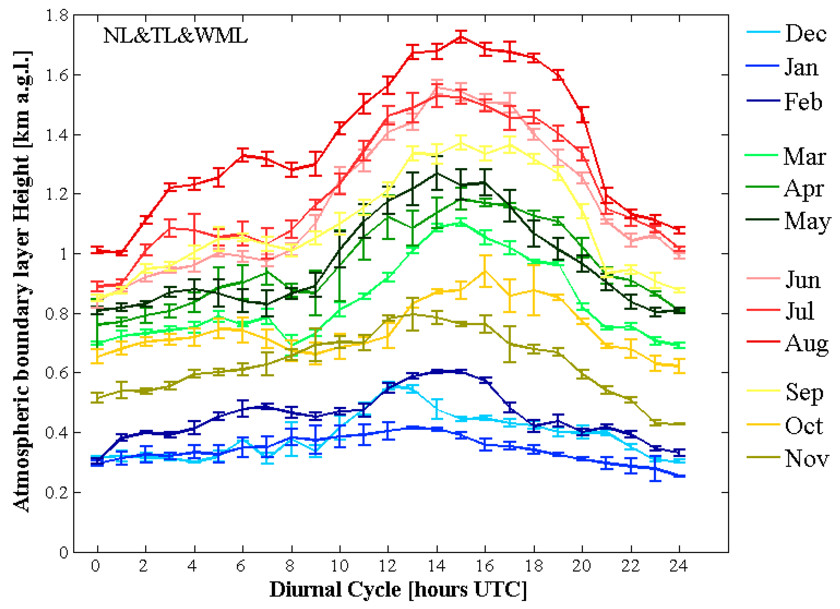
6.1. Monthly Variability of the Average Diurnal Cycles of the Boundary Layer Height

The monthly average diurnal cycles of ABLH were derived for a subset of the clear-sky diurnal cycle data listed in brackets in Table 3. They were calculated separately for the ABLH values obtained as the NL, TL, and WML versus the RL, TL, and WML (definition in Table 1) to assess the differences related to the nocturnal and the residual boundary layer. As expected, the diurnal cycles that included the nocturnal layer information, shown in Figure 8, were more pronounced than the diurnal cycles including information on the residual layer (the latter not shown for brevity). The ABLH maximum values in each cycle for 12 months were mainly distributed from 12:00 until 15:00 UTC, except for the winter months. The significantly higher nocturnal boundary layer in August than December can be attributed to the solar position and zenith angle, which leads to an earlier sunrise and a late sunset in the summer months. Thus, it affects the solar radiation reaching the surface, and hence, the surface temperature, causing a higher boundary layer in summer than in winter. In Warsaw, nighttime in summer lasts about 7 h (or less) and in winter about 14 h (or more), so that in summer, one cannot expect a strong cooling effect at night. Therefore, the difference of 500 to 700 m in the ABLH derived at night in summer and winter is plausible.

The monthly average diurnal cycles indicated strong seasonal changes. The most spectacular was the abrupt change of the winter boundary layer cycle shape and height (Figure 8, in blue), which maintained a very low diurnal variability in December, January, and February. A well-pronounced diurnal cycle of the following spring months is depicted (in green). This sharp winter-to-spring cycle change was related to a well-pronounced pre-spring season (discussed below).

The diurnal cycles obtained for spring and summer indicated a smooth and mild month-to-month transition to higher ABLH values, with an increase of the heights during both the day and nighttime. The diurnal cycle for August (Figure 8, in red) was found to be the highest; it stands out from the others in terms of the ABLH values but not the shape. The August diurnal cycle remained practically unaffected by the uneven data sampling—the highest probe for August 2015 (48/19 cases). Excluding the August 2015 data from the diurnal cycle of August (not shown for brevity) revealed only a slightly flattened shape (30 to 90 m lower ABLH values between 12:00 and 20:00 UTC).

The autumn diurnal cycle of September (Figure 8, in beige) resembled the summer cycles of June and July (Figure 8, in pink and red), which indicates a prolongation of the summer season at the cost of autumn. The similarity of the September cycle to the summer cycles is naturally related to the meteorological conditions being more like those in summer. The prolongation of summer in Poland that is manifested in the derived diurnal mean cycles of 2008 to 2018 was reported in other studies (e.g., [77]). The remaining autumn cycles (Figure 8, in yellow) were significantly lower, not only from the September cycle, but generally from all spring and summer cycles. This indicates a somewhat smooth transition to the winter season. Still, the October and November diurnal cycles have distinctly different shapes from all winter cycles.

The much higher spring cycles than the winter cycles and the well-separated height in the autumn cycles from the winter cycles indicate a very short and well-defined winter season. The January cycle has a flat shape. Taking into account the equal representatives of the data for the hour of day (the majority of samples obtained for ceilometer observations in 2008 to 2013), this can be explained by the urban heat island effect.

The urban heat island (UHI) means that the temperature within the urban area is significantly warmer than in the surrounding rural areas [76]. The effect is due to both human activities in the city (traffic, combustion, etc.) and the differences between the land surfaces in the city and the rural areas [78]. At night, the absence of solar heating (no strong atmospheric convection) normally leads to the stable boundary layer [1,2,3]. During UHI conditions, the inversion traps the urban air near the surface and keeps it warm from the urban surfaces. This results in warmer nighttime air temperatures that prevent a strong decrease of the urban boundary layer height after sunset [79]. The mean yearly intensity of the UHI index (difference of the minimum daily temperature for the urban area to the value of the minimum daily temperature for the suburb area) reaches over 2 °C in the city center over Warsaw. The very center of the city is warmer in the night by 2.5 °C compared to the outskirts [78]. The UHI is most effective and intensive in wintertime, at night or before dawn [78]. The wintertime diurnal cycles may also be affected by biases due to an occurrence of the nocturnal layers below the detection range of the ceilometer or lidar (195 m), although this is expected to have a minor effect on the retrievals in comparison with the heat island effect.

In general, the diurnal cycles showed an increase during the transition from the spring months (0.7–1.2 km) to reach their highest values in the summer months (0.9–1.7 km). Thereafter, in autumn, a decline of the mean monthly ABLHs was observed (0.6–1.3 km). The lowest mean values (≤0.6 km) occurred, as expected, in the winter months. This is, in general, in agreement with the average ABLH summer and winter values of, respectively, 1.5 and 0.7 km reported previously for Warsaw [29,52].

According to the Koeppen–Geiger climate classification system (maps available at http://koeppen-geiger.vu-wien.ac.at), the climate over Poland has changed. In 1951 to 1975, western Poland was under the Cfb climate (defined as warm temperate humid with warm summer) and eastern Poland was under the Dwd climate (defined as boreal extremely continental with dry winter). In the following decade, the Cfb climate was already over the whole of Poland [80]. Traditionally, the climatic and astronomical seasons are not identically defined for Poland, as there are two additional pre-seasons regarded as being present in Poland’s climate: The pre-winter, with significant cooling in November, and the pre-spring, with significant warming at the turn of February and March [77]. In the obtained monthly mean diurnal cycles, the pre-spring season was evident (exceptionally high March cycle; Figure 8, in light green). The autumn diurnal cycle of November was not very low, as expected as representing the pre-winter season (Figure 8, in dark yellow). The change of the climate seasonality of Poland [80] is in accordance with the ABLH cycles resembling the very warm spring [77], as well as the prolonged summer into the month of September.

6.2. Annual Variability of the Monthly and Seasonal Mean Boundary Layer Height

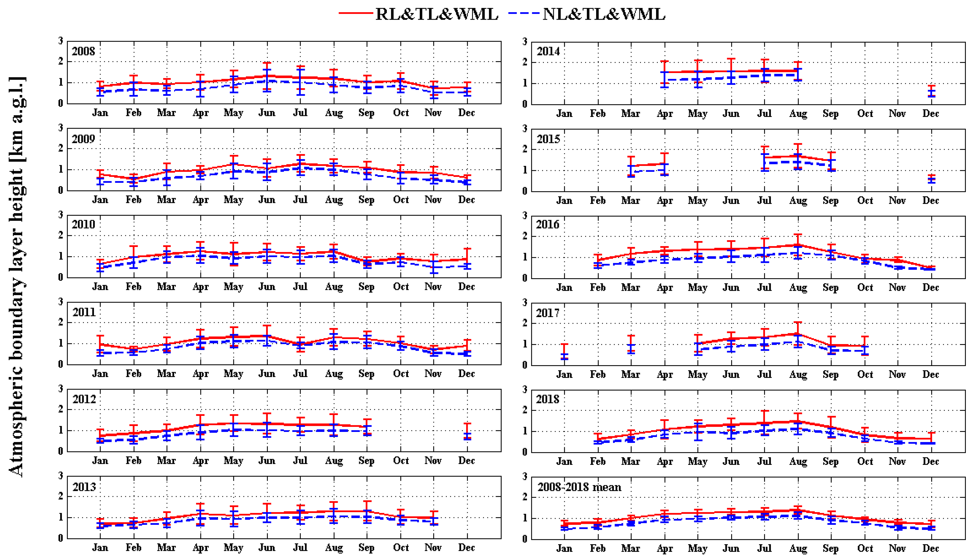
The monthly mean ABLH values with standard deviations were calculated from the 1841 daily evolution cycles obtained in all-weather conditions. Note that the obtained temporal variations may be affected by data availability (Table 3). The annual variability of the monthly mean ABLH values from 2008 to 2018 was plotted in Figure 9, separated into the RL, TL, and WML average (in red) and the NL, TL, and WML average (in blue). Because the residual layers can be valuable for the interpretation of pollution concentrations observed within the ABL [55,59], such a separation can be useful for future studies. As expected, the heights of the NL, TL, and WML were lower, but the trend of both was similar. The monthly annual changes from 2008 to 2011 were observed for all months, whereas after 2011, for some months the mean values could not be obtained. In general, the monthly mean ABLHs showed a slight increase from the spring months (MAM) to the summer months (JJA), where the mean ABLH increased to its highest values, with the mean exceeding 1 km. The lowest mean ABLH values appeared mainly during the winter months (DJF), with mean values of less than 1 km for all years. For the autumn months (SON), a similarity with either the winter or spring months was captured. From 2008 to 2013, the fluctuations of ABLHs generally remain around 1 km. In 2014 and 2015, high monthly mean ABLHs (>1.5 km) were derived, which can be partly attributed to the most missing data in these two years (a total of about 50 days per year).

The year-to-year monthly mean ABLHs were the lowest for the winter of 2016 and 2018, and the highest for the springs and summers of 2014, 2015, and 2016. This should be at least partly attributed to the decadal activity of the ENSO, resulting in global atmospheric heating (El Niño) or cooling (La Niña). The monthly mean ABLHs are in accordance with the moderate-to-strong El Niño in 2014–2016 and the moderate La Niña in 2010–2012, both reported by the NOAA Oceanic Niño Index (available via http://origin.cpc.ncep.noaa.gov/products/analysis_monitoring/ensostuff/ONI_v5.php, last access: 11 December 2019). The strong El Niño can result in highly increased temperatures and droughts in Europe [81,82]. At the same time, the resulting prolonged increase of the surface temperature due to droughts and heat waves can cause a higher boundary layer [8,9,10,11].

These effects can be seen on the scale of the annual cycle (Figure 9). The extreme summer heat wave was observed over Europe during July 2015 and resembled exceptionally high values for the two following months [82,83,84]. A European heat wave event was also reported for September 2016 [11]. The surface air temperature monthly means with anomalies (relative to the monthly average calculated for the period 1981–2010) are provided from September 2015 until the present month by the ERA-Interim ECMWF Copernicus Climate Change Service (maps available via https://climate.copernicus.eu/resources/data-analysis/average-surface-air-temperature-analysis, last access: 11 December 2019). The monthly mean ABLHs depicted in Figure 9 are in accordance with the surface air temperature monthly anomalies, and also the observed variability of the monthly mean ABLHs are related to the average surface air monthly temperature, reported therein.

In

Table 4. The seasonal mean ABLH values obtained from the PollyXT lidar and the CHM15k ceilometer data using the wavelet covariance transform (WCT) method for observations conducted in all-weather conditions over Warsaw, within the period from 2008 to 2018. Mean values for seasons with less than 10 measurement cycles are indicated in italics, being regarded as statistically not representative. Merging and homogenization were applied to lidar data from November 2013 to December 2018.

	Spring (MAM) Mean ± std [km]	Summer (JJA) Mean ± std [km]	Autumn (SON) Mean ± std [km]	Winter (DJF) Mean ± std [km]
2008	1.02 ± 0.58	1.24 ± 0.72	0.96 ± 0.61	0.81 ± 0.50
2009	1.00 ± 0.56	1.16 ± 0.64	0.96 ± 0.56	0.72 ± 0.43
2010	1.15 ± 0.69	1.17 ± 0.60	0.83 ± 0.50	0.75 ± 0.59
2011	1.16 ± 0.65	1.18 ± 0.68	0.98 ± 0.58	0.85 ± 0.49
2012	1.18 ± 0.63	1.28 ± 0.69	1.17 ± 0.58	0.83 ± 0.58
2013	1.06 ± 0.64	1.24 ± 0.64	1.11 ± 0.57	0.70 ± 0.41
2014	1.54 ± 0.57	1.58 ± 0.60	× (0)	× (0.65)
2015	1.24 ± 0.48	1.61 ± 0.51	× (1.30)	× (0.61)
2016	1.29 ± 0.59	1.46 ± 0.60	1.09 ± 0.49	0.67 ± 0.34
2017	1.01 ± 0.43	1.35 ± 0.57	0.92 ± 0.41	0.65 ± 0.36
2018	1.09 ± 0.41	1.40 ± 0.53	0.85 ± 0.45	0.63 ± 0.25
Total	1.16 ± 0.16	1.34 ± 0.15	0.99 ± 0.11	0.73 ± 0.08

, the variability of the seasonal mean ABLH values in each year, (winter months (DJF), spring (MAM), summer (JJA), and autumn (SON) for the years of 2008 to 2018 is given. In autumn and winter of 2014 and 2015, the values indicated in brackets cannot be regarded as representative of the seasonal mean (defined as at least 10 days within the 3-month-long season of each year, with at least 6 h at daytime and 6 h at night). Still, these values are given to provide rough information but not as a seasonal mean. The decadal seasonal mean ABLH reached its largest values in the summertime, with an altitude of 1.34 km, and the lowest values in the wintertime of 0.73 km. The mean spring and autumn ABLHs were 1.16 and 0.99 km, respectively.

The seasonal mean ABLHs, listed in Table 4, indicate for most of the years that for spring and summer the values were above 1.1 km, for autumn below 1.1 km, and during winter below 0.8 km. However, after 2014, the mean height in the spring and the summer seasons was notably higher (200–300 m) than those of the previous years while for the winter season, it was further decreased (of about 200 m). For the years 2008–2013 and 2017–2018, the differences in the seasonal mean ABLH values were relatively small and remained within 400 m, but for 2014–2016, those differences were about twice larger, which should not be solely attributed to the absence of data in 2014 and 2015. The 10-year mean seasonal ABLH was 1.16 ± 0.16 km for spring, 1.34 ± 0.15 km for summer, 0.99 ± 0.11 km for autumn, and 0.73 ± 0.08 km for winter.

If any sampling biases were to critically affect the year-to-year variation of all mean ABLHs in the four seasons for the years 2014–2018 (derived with lidar only), they would be expected to reveal higher values than those of 2008–2012 (derived from ceilometer only), as a systematic error. This is not the case, as, e.g., the results for the winters of 2013–2018 and springs and autumns of 2017–2018 are lower than those derived from 2008 to 2012. As for the decadal mean seasonal variability of ABLH, they are least affected by biases and these values can be used as a reference.

6.3. Variability of Yearly Mean Well-Mixed, Nocturnal, and Residual Boundary Layer Height

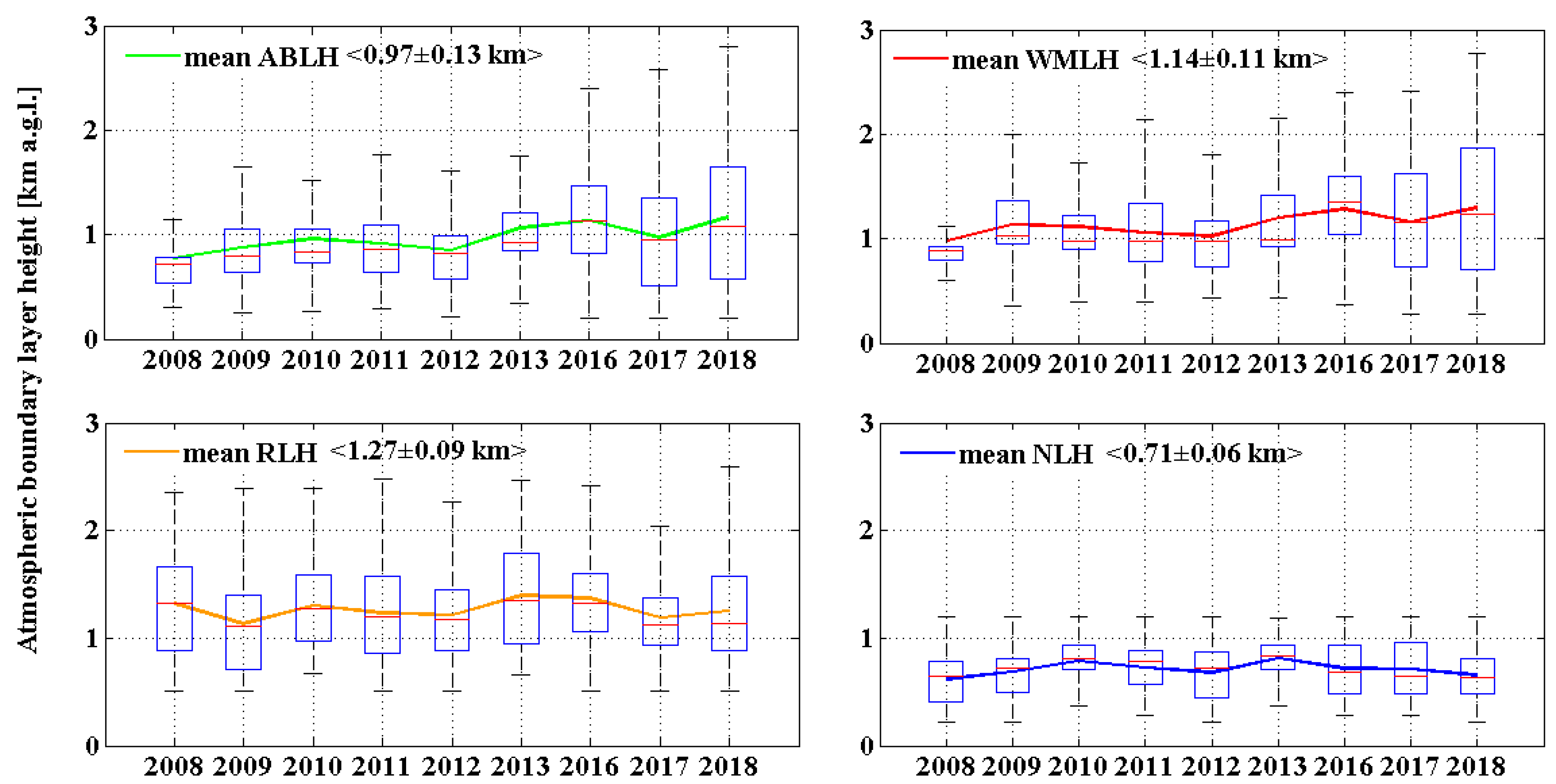
The box and whisker plots depicted in Figure 10 summarize the variability in the annual mean ABLH values derived for the subset of the clear-sky data (346 days). In this figure, the solid lines indicate the annual mean ABLH obtained for each year, except for the years 2014 and 2015, for which calculation of the annual mean was not possible (too low data availability in autumn and winter months; Table 3). The annual mean ABLHs (Figure 10, in green) were the highest in 2016 and 2018. Overall, the annual mean ABLHs were between 0.8 and 1.3 km.

The annual mean WML, NL, and RL in Figure 10 show that the mean annual WML values have strong similarities with the mean annual ABLHs, with the peaks in 2016 and 2018. The mean annual NL and RL values followed different trends with no distinct peaks; the NL below 0.83 km and the RL between 1.13 and 1.39 km. Lower residual layer heights, being in the range 0.7–1.4 km, were reported for Paris, France and in the range 0.5–0.9 km for Moscow, Russia [85]. Over Houston, Texas, the nocturnal boundary layer height was reported at 0.25 km throughout the year while the convective boundary layer heights were at 1.1 km in winter and 2 km in summer [55]. Such differences are not unexpected and can be attributed to the diverse climatic conditions at these sites. Two of them have a temperate climate (1980–2016), i.e., Houston (Cfa) and Paris (Cfb). The two others have a continental climate (1980–2016), i.e., Warsaw (Dfb) and Moscow (Dfc) [80]. As for the derivation of the nocturnal boundary layer in Warsaw, the lower detection limit at 195 m could have led to a slight overestimation of the derived values. However, even for scanning lidars, where the overlap is claimed to play a negligible role due to the measurement geometry, heights of the boundary layer between 0.5 and 2.4 km were reported for August to October over Slovenia [86], considered a continental climate of the Dfb type, such as Warsaw [80].

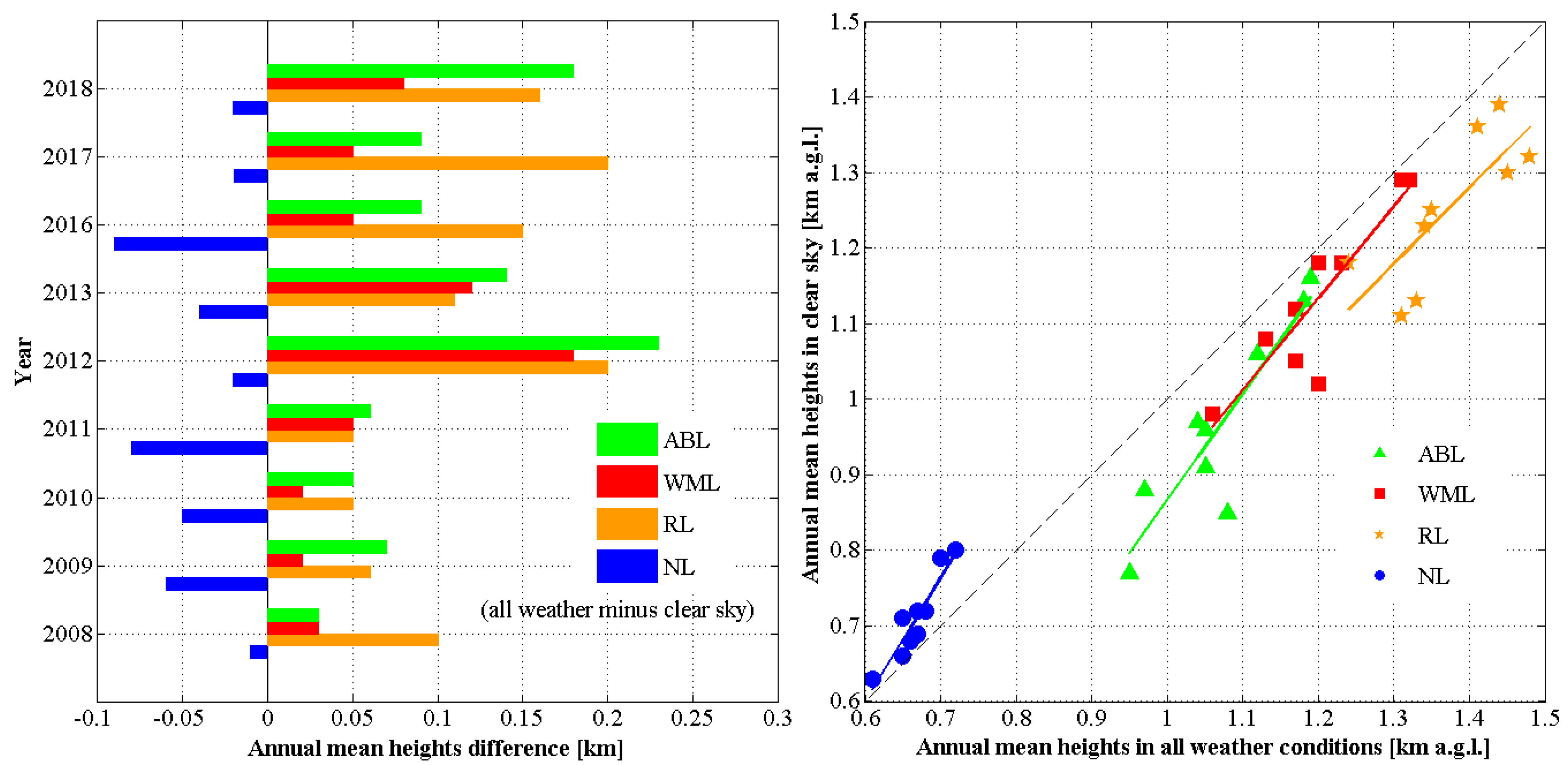
The mean yearly ABLH, WML, RL, and NL values were obtained for the total number of available data (1841 diurnal cycles) as well as for the subset of clear-sky data (346 diurnal cycles). This was done to assess expected differences between those two samples, whereby the temporal separation of the data was taken into account. The bias of the ABLH retrieval performed in the clear-sky and boundary layer clouds is related to clouds forming directly above the boundary layer itself (e.g., in the entrainment zone, <3 km [1,2,3]). The other types of clouds, e.g., generated by the mesoscale frontal weather systems, were not considered (they have been screened, as, in the majority of situations, they are detached from the boundary layer). Therefore, the difference of the annual mean ABLH derived for the all-weather conditions and the clear-sky conditions represents this bias. In Figure 11, right subfigure, the bias is below 230 m for the ceilometer (2008–2012) and 70 m for the lidar (2016–2018). For the annual mean values of the WML, RL, and NL, the bias is below 250 m for both instruments. Measurements with each instrument indicate different cloud effects, which can be partly attributed to the difference in their design and partly to various atmospheric conditions. The signal-to-noise ratio is lower for the ceilometer than lidar due to the lower laser power, resulting also in a shorter range of the ceilometer signals [38,62,69]. Therefore, lidar is more sensitive for the aerosol and cloud detection. On the other hand, the differences seen for the cloudy conditions in Figure 11, also have to do with the captured annual variations in the atmospheric conditions for the all-weather data depicted in Figure 9.

In general, with an increase of the annual mean ABLH, increased heights of the WML, RL, and NL were observed (Figure 11, left subfigure). The heights of the ABL, WML, and RL were higher for the all-weather conditions than on the clear-sky days. Conversely, the height of the NL under the all-weather conditions was found to be lower compared to its height in the clear-sky days (Figure 11, right subfigure). Both, an increase in the cloud cover at night and an urban heat island under clear-sky conditions can lead to a deeper ABLH at night. For the data sample collected and analyzed in this paper, the second process seems to be more efficient in Warsaw.

The ABLH under the UHI is the result of processes driven not only by the local surface conditions but also by the regional atmospheric structures [87]. In the literature, there are some idealized realizations of boundary layers, such as, e.g., in [1,2,3]. Reality is more complicated due to differences in the heat sources, heat capacities, and surface roughness, e.g., the classic evolution of a daytime convective boundary layer distribution as affected by advection of dry air and gravity waves was reported by [88]. In the current paper, not all those regimes were studied.

Several studies reported in the literature are limited to the clear-sky daytime conditions and provide only the maximum ABLH. For instance, for an urban continental site in Leipzig, Germany, the afternoon ABLHs corresponding to the well-mixed layer height were reported, with a maximum value at approximately 1.4 km in spring, 1.8 km in summer, 1.2 km in autumn, and 0.8 km in winter, as derived from single-year observations [25]. The maximum ABLHs in the current study were found even beyond 2 km in Warsaw, Poland. The mean ABLHs in Warsaw, calculated for the different seasons and years, are reported as being in the range of circa 250 m lower than the maximum values reported for Leipzig [25]. The annual cycle of convective boundary layer heights in summer and winter reported above the Swiss Plateau [44] had values far from those derived for Warsaw and Leipzig. Over Neuchâtel, Switzerland, the nighttime residual heights detected with lidar were reported as changing from 0.5 to 1.5 km [21]. In Barcelona, Spain, the well-mixed boundary layer was reported between 0.3 and 1.45 km in summer and between 0.39 and 1.42 km in winter, showing almost no seasonal difference, unlike in Warsaw [37]. The discrepancies of the values reported within the current study and the mentioned publications are attributed to the differences in the localization of cities/regions (coastal, plateau, inland). Also, the distinct climatological conditions add to these differences.

It has been reported that the aerosol optical properties derived within the boundary layer (divided to the different temporal regimes: WML, TL, NL, and RL) show significant differences in Warsaw, especially for the diurnal variation [52]. Thus, high-quality retrieval of the ALBH at daytime and nighttime is crucial. Note that the analysis of Figure 11 relies on cloud characteristics (cloud cover, cloud base height, cloud type), therefore its interpretation is not straightforward.

The dependence of the temperature on cloud cover is strong in the middle latitudes [89]. During the daytime, an increase in cloud cover can restrict the incoming solar radiation, and thus, decrease surface temperatures. However, at night, an increase in the cloud cover is expected to reduce the long-wave cooling (i.e., warmer surface temperatures), and thus lead to a deeper ABLH at night (e.g., in [14]). The cloud cover and type influence the boundary layer characteristics; the mixed layer height may vary distinctly depending on the frequency and cloud types present [53]. Moreover, the global temperature rise, reinforced in urbanized areas by the anthropogenic heat flux, leads to an intensified convection process and increased precipitation (especially torrential rain), causing thermal and hydrological hazards in large conurbations. The areas currently exposed to thermal and urban flood hazards in Warsaw were identified and assessed in the recent work of [83].

6.4. Frequency Distribution of Daytime and Nighttime Boundary Layer Height

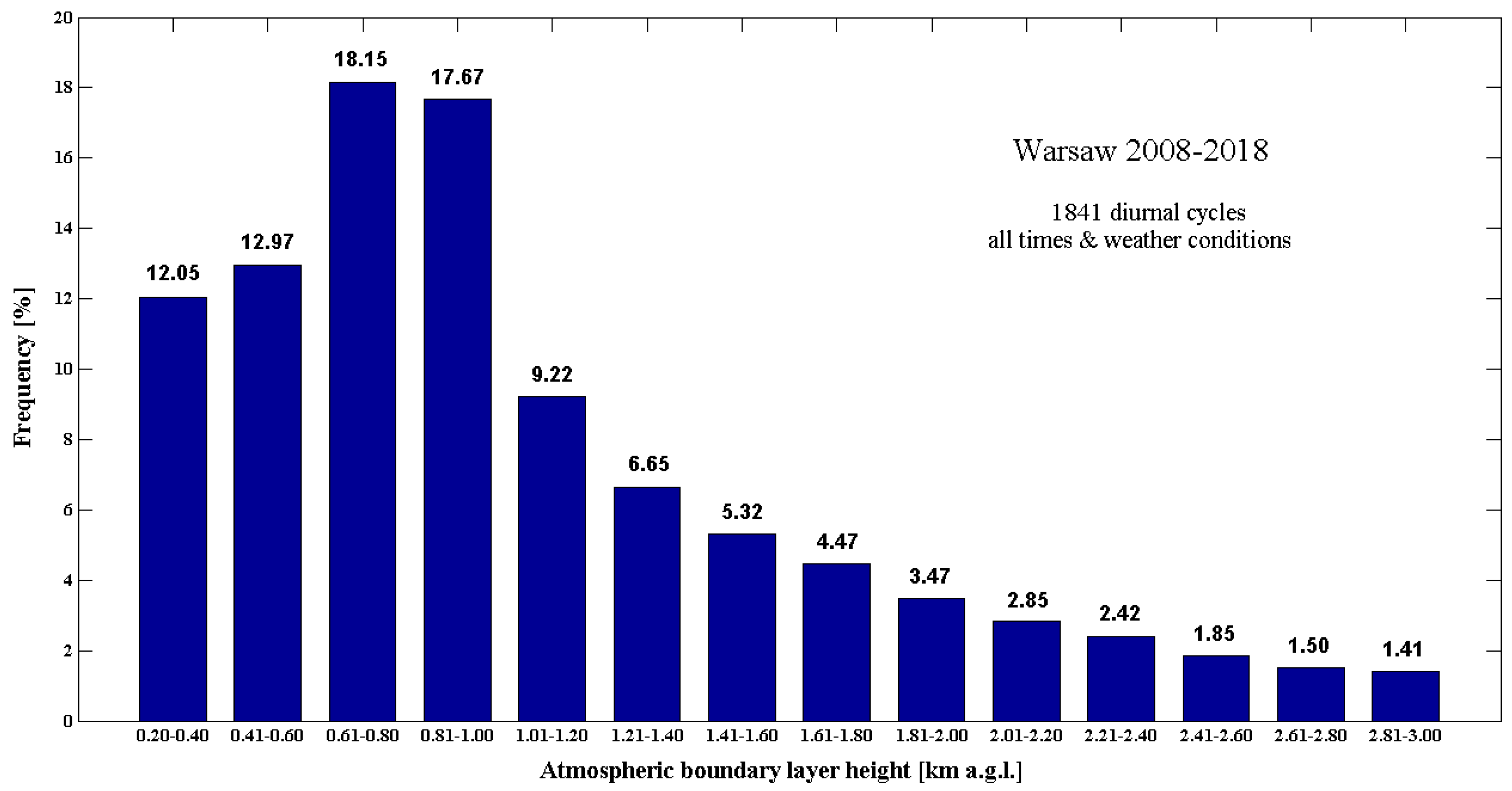
In order to indicate on the total distribution of ABLH within 2008–2018 over Warsaw, the histogram of the frequency distribution of the ABLH derived for the 1841 diurnal cycles is depicted in Figure 12. All hours were used, hence there is no bias for any particular time of day.

The asymmetric positive skew distribution with the right tail significantly longer and with the mean value higher than the median was obtained. The ABLH values up to 1 km had a frequency of more than 60% of the entire data sample. The ABLH distribution was dominated with the values between 0.6 and 1 km (the class 0.6–0.8 km was the most frequent, with the percentage of 18.15%, followed by the class 0.8–1 km, with a frequency of 17.67%). Then, the values between 0.2 and 0.6 km were significantly frequent (class 0.4–0.6 km (12.07%), followed by the class 0.2–0.4 km (12.05%).

For higher altitudes (>1 km), as the ABLH increased, their occurrence gradually decreased. Rarely, the ABLH values reached altitudes of 2.4 to 3 km, which accounts for only 4.76% of the whole data sample. The obtained frequency distribution can be used as a reference for comparison with other measurement sites, e.g., as in [74], whereby a distinction can be made between, e.g., the daytime and nighttime distributions.

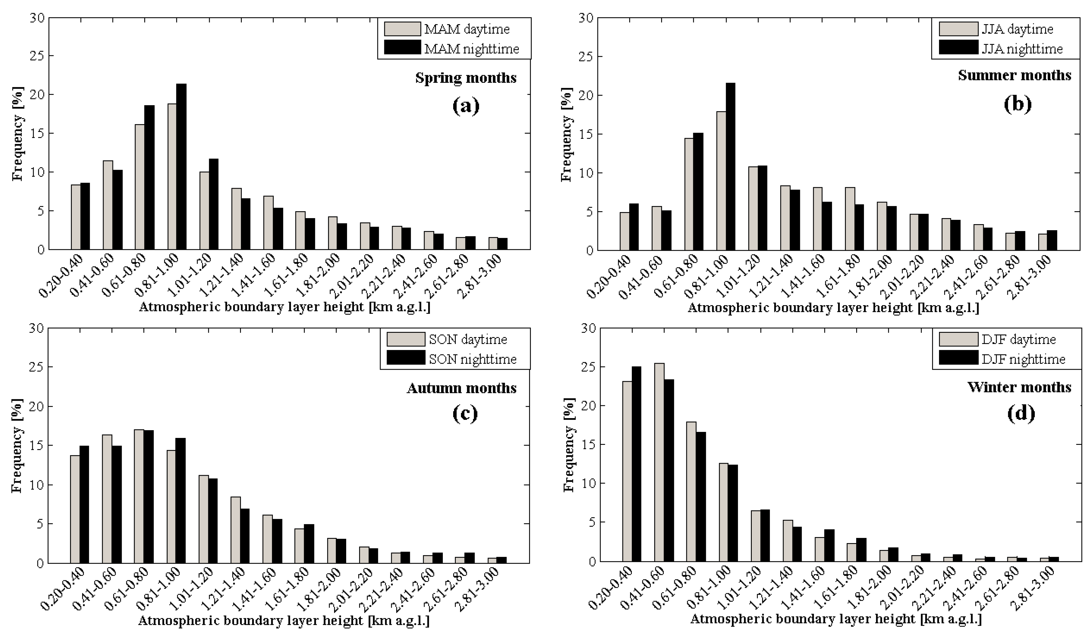
Additionally, a detailed investigation of the ABLH frequency distribution was performed with respect to the time of day and for the different seasons of the year. The frequency distribution histograms are plotted in Figure 13, where the daytime frequencies are given in grey and nighttime in black.

In spring and summer (Figure 13a,b), the ABLHs were most often within the range of 0.6 to 1 km; this being a distinct maximum of the occurrence frequency of 30% to 40%. In general, at the ranges up to 1.2 km, the ABLH occurrence at nighttime was practically always slightly higher than at daytime (expect for winter); above this height, an opposite trend occurred. For winter and autumn, no such trends are observed. In the summer months (Figure 13b), a visibly higher frequency of ABLHs over 1.4 km was observed, as compared to the other seasons. This is consistent with the fact that in summer, more solar radiation is expected to be absorbed by both land and atmosphere, which is then attributed to a stronger variation of the heat flux, turbulence, and more active energy exchange. Consequently, this leads to a lofted ABLH during the summer months. On the contrary, most of the ABLH values during the winter season (Figure 13d) occurred within the range between 0.2 and 0.6 km (~50%, at both, day and night). In winter, the occurrence of ABLH above 1.8 km is negligible (<5%). During the autumn months (Figure 13c), the distribution of the ABLH values within 0.2 and 1 km was well balanced, with frequencies between 14% to 16% (in total ~60%), at both, day and night.

Notably, a few ABLHs above 2.8 km were found in all four seasons, regardless of during the daytime or nighttime. A reasonable explanation for such observations at daytime may be stronger turbulent mixing and exchange processes between the surface and the free troposphere, which contribute to a relatively high ABLH between noon and the late afternoon (e.g., [52,75]). As for an ABLH above 2.8 km during the night, it may be attributed to at least to two reasons. Either there were aerosols remaining after sunset, which developed a residual layer when the temperatures declined during the course of the night (e.g., an extremely high boundary layer (up to 3 km), driven by a severe heat wave conditions, discussed in detail in [11]). Or the tested boundary layer retrieval methods (GDT, STD, and WCT) were, to some extent, influenced by the atmospheric stratification (particularly in complex advection-pronounced conditions), as these algorithms always find the largest signal change. These factors, each alone or in interplay, may have led to a higher ABLH during the nighttime. The ABLH values found above 2.8 km in autumn and winter are considered as limitations of the applied methodology. Note that no passing clouds appeared for the ABLHs found at the range 2.8–3 km.

As expected for an urban continental site in Central–East Europe, a strong seasonal variability of the ABLH distribution (in height and shape) was observed. The spring distribution (Figure 13a) clearly dominated the total distribution (Figure 12). The ABLH distribution peak and shape varied strongly with the seasons. The peak of ABLHs between 0.6 and 1 km was observed in spring, then it became sharper (0.8–1 km) in summer, just to flatten in autumn as an equal spread between 0.2 and 1 km, and finally to peak in winter at 0.2 to 0.6 km. The study of the boundary layer height over Europe, derived based on the bulk-Ri number from the rawinsondes, revealed that 50% of all ABLH values at daytime are generally <1 km and at nighttime <0.5 km [51]. The seasonal patterns for the daytime and nighttime can significantly differ; daytime heights larger in summer than in winter, but the nighttime heights larger in winter, were reported by [45]. These variability trends obtained over Europe are similar to the results for Warsaw. The differences are therefore due to the physical basis for instruments’/algorithms’ working principles as well as the specific weather or air quality-related episodes.

7. Conclusions

Measurements conducted at the same wavelength (1064 nm) using the CHM15k ceilometer (2008 to 2013) and the PollyXT lidar (2013 to 2018) were homogenized, combined, and deployed to determine the atmospheric boundary layer characteristics. The height, structure, and evolution of ABLH were obtained for 1841 observations of diurnal cycles over the city center of Warsaw, Poland. For comparative study, 4 months of collocated ceilometer and lidar measurements (July–October 2013) were chosen. For this period, the ABLH was determined also from the WMO rawinsondes launched at noon and midnight in Legionowo (25 km, North).

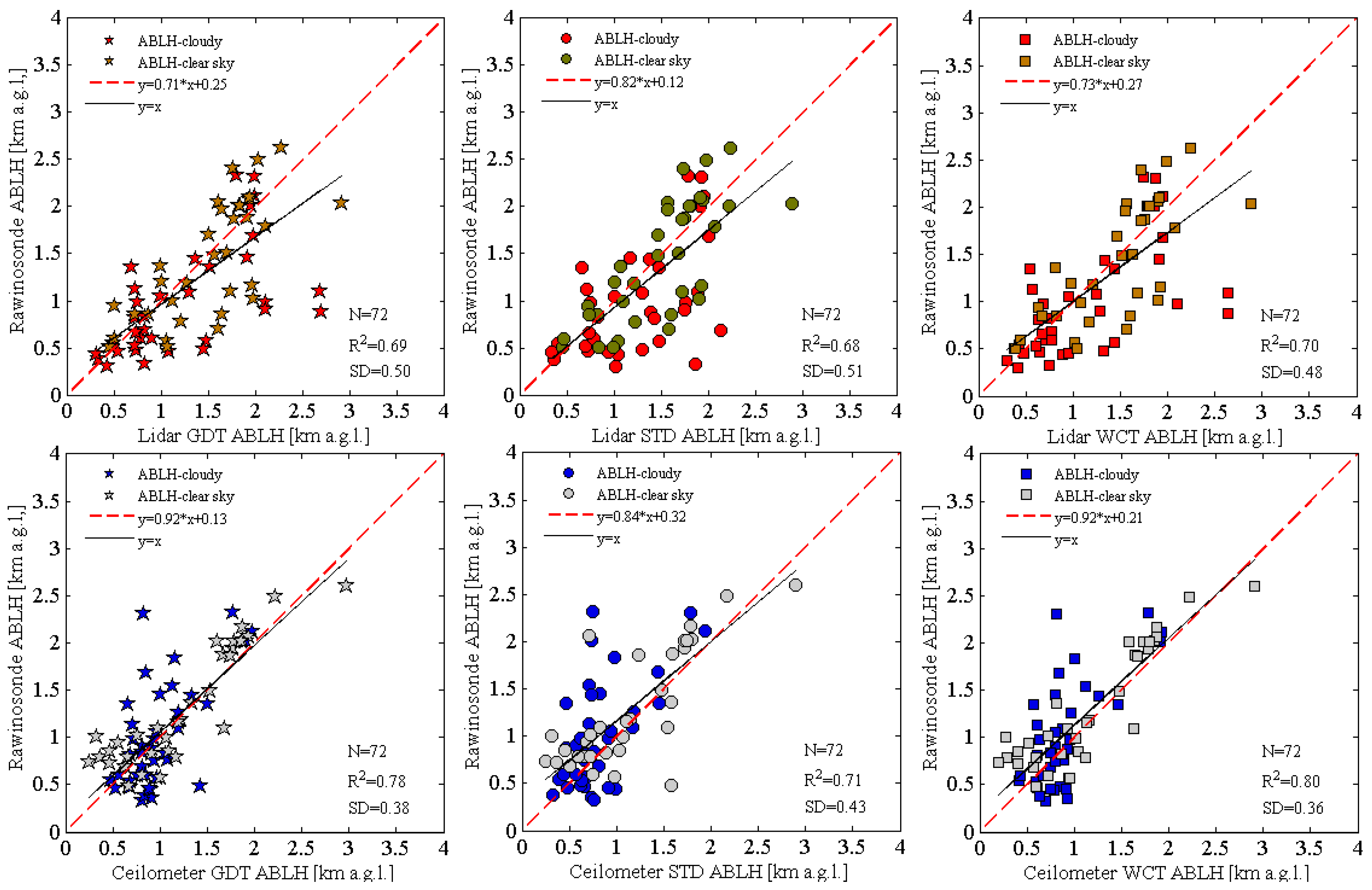
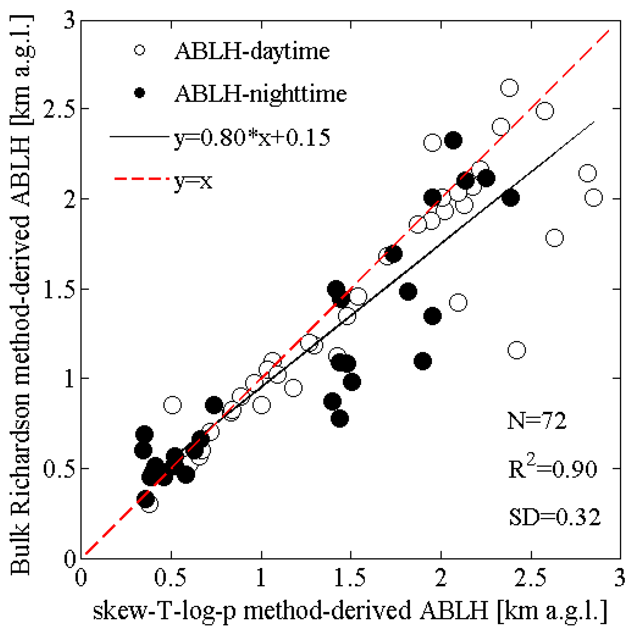
The bulk Richardson (bulk-Ri) method was found more favorable than the skew-T-log-P for ABLH detection from rawinsondes. The lidar and ceilometer ABLHs in Warsaw, obtained with the gradient method (GDT), standard deviation method (STD), and wavelet covariance transform method (WCT), exhibited relatively high correlations (R² of 0.68–0.80 with SD of 360–510 m), in comparison with the rawinsondes ABLHs obtained by using the bulk-Ri method. The WCT results indicated an ability to detect ABLHs more accurately than the GDT and the STD methods. The ceilometer-derived ABLHs were assessed as more reliable (more similar to the rawinsondes’ retrievals).

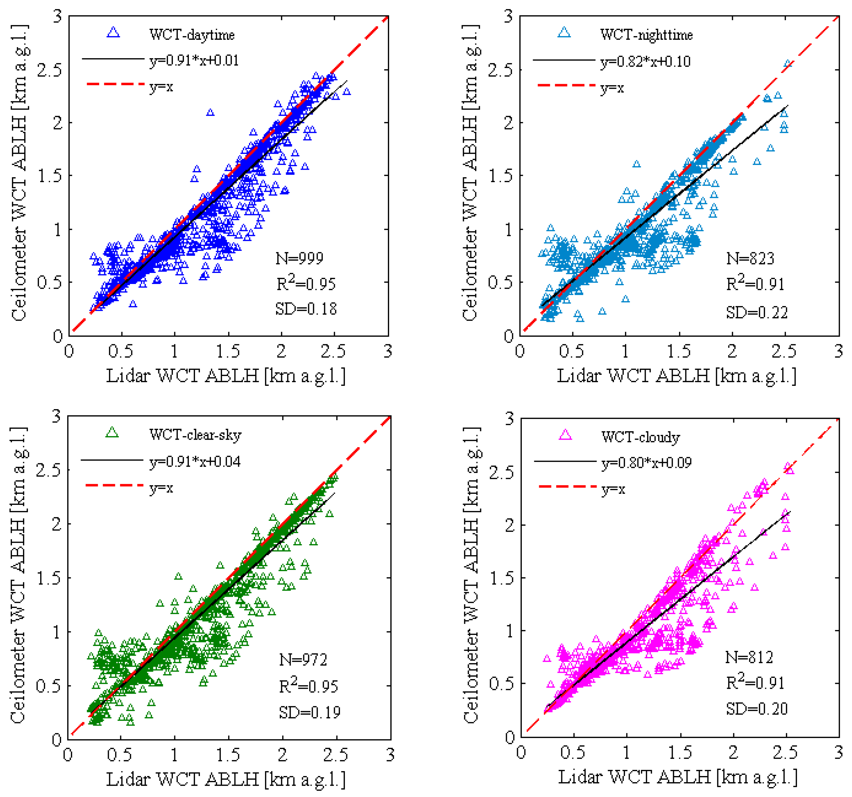
The lidar–ceilometer direct comparisons revealed significantly higher correlations (R² of 0.93–0.94 with SD of 190–200 m). The algorithms developed for homogenization of the ceilometer and lidar datasets reduced this bias to only 110 m. The WCT method performed well at day and nighttime in different conditions. The bias of ABLH retrieval in the clear-sky to the cloudy-conditions was <230 m for ceilometer and <70 m for lidar. Currently, this bias cannot be corrected.

The statistical analysis of the long-term datasets (2008–2018, 1841 diurnal cycles) revealed that the annual cycles of the monthly mean ABLHs (calculated for all days; clear sky and with boundary layer clouds) in Warsaw ranged from approximately 0.6 to 1.8 km, throughout the years. The lowest monthly mean ABLHs were derived for the winters of 2016 and 2018, and the highest for the springs and summers of 2014, 2015, and 2016.

The average monthly diurnal cycles of ABLH derived for clear-sky data showed pronounced changes: (i) A gradual transition from spring months (0.7–1.2 km) to summer months (0.9–1.7 km) with maximum values in August; (ii) the cycle for September (autumn) strongly resembled the cycles of June and July, indicating prolongation of the summer season; (iii) a decline of mean monthly ABLHs in mid-autumn (0.6–0.9 km) and a smooth transition to winter; (iv) the lowest mean values (below 0.6 km) in the winter months with spectacular flattening of the January cycle shape; and v) the abrupt change between the winter and spring season due to the regional climate change.

The annual mean ABLH in clear-sky conditions over Warsaw was obtained for the years from 2008 to 2018, except for 2014 and 2015 (significant absence of measurements in autumn and winter months). The annual mean ABLHs were maintained between 0.77 and 1.16 km, whereby the annual mean well-mixed boundary height ranged from 0.98 to 1.29 km, the annual mean residual layer from 1.13 to 1.39 km, and the annual mean nocturnal layer from 0.62 to 0.81 km. The seasonal mean ABLH was 1.16 ± 0.16 km in spring, 1.34 ± 0.15 km in summer, 0.99 ± 0.11 km in autumn, and 0.73 ± 0.08 km in winter.

The frequency distribution revealed ABLHs occurring below 1 km as constituting more than 60% of the total data. A strong seasonal variability of the ABLH distribution was observed (the spring distribution clearly dominated the total distribution). ABLHs between 0.6 and 1 km were most frequent during spring and summer (>35% and >30% of all data, respectively). In autumn, the distribution flattened (60% of data equally spread between 0.2 and 1 km). In winter, the distribution peak was between 0.2 and 0.8 km (~70% of data) to fall quasi-exponentially above 0.8 km.

The nighttime and daytime ABLH distribution revealed significant differences; heights reaching beyond 1.2 km were more often observed at daytime in all seasons (except winter). An opposite trend was observed below 1.2 km. Regardless of the time of day, the ABLHs above 1.2 km are more frequent in summer than during the other seasons while the ABLHs below 0.6 km account for the main part of the observations during the winter and autumn months. Due to the occurrence of residual lofted aerosols, the ABLHs exceeding 2.8 km were observed sporadically regardless of the season (<5% summer, <1% winter).

Recently, available methods for the ABLH retrieval from the lidar and ceilometer observations were summarized in a review paper [18], which concludes that although many techniques have been proposed in the literature, it is still impossible to recommend a technique that is suitable in all atmospheric scenarios. In the current paper, an approach of scaling the lidar-derived ABLH to homogenize them with the ceilometer-derived ABLH was proposed and was applied with success, providing comparable products from both instruments.

References

1. Sorbjan, Z. Structure of the Atmospheric Boundary Layer; Prentice Hall: Englewood Cliffs, NJ, USA, 1989. [Google Scholar]
2. Garratt, J.R. The Atmospheric Boundary Layer; Cambridge University Press: Cambridge, UK, 1992. [Google Scholar]
3. Stull, R.B. An Introduction to Boundary Layer Meteorology; Springer Science & Business Media: Berlin, Germany, 2012; Volume 13. [Google Scholar]
4. Climate Prediction Center/NCEP, ENSO: Recent Evolution, Current Status and Predictions. 16 December 2019. Available online: https://www.cpc.noaa.gov/products/analysis_monitoring/lanina/enso_evolutionstatus-fcsts-web.pdf (accessed on 11 December 2019).
5. Sungsu, P.; Clara, D.; Michael, A.A. Estimation of the Surface Heat Flux Response to Sea Surface Temperature Anomalies over the Global Oceans. J. Clim. 2005, 18, 4582–4599. [Google Scholar]
6. Park, S.; Alexander, M.A.; Deser, C. The Impact of Cloud Radiative Feedback, Remote ENSO Forcing, and Entrainment on the Persistence of North Pacific Sea Surface Temperature Anomalies. J. Clim. 2006, 19, 6243–6261. [Google Scholar] [CrossRef] [Green Version]
7. Stuecker, M.F.; Jin, F.-F.; Timmermann, A.; McGregor, S. Combination mode dynamics of the anomalous northwest Pacific anticyclone. J. Clim. 2015, 28, 1093–1111. [Google Scholar] [CrossRef]
8. Loughran, T.F.; Pitman, A.J.; Perkins-Kirkpatrick, S.E. The El Niño–Southern Oscillation’s effect on summer heatwave development mechanisms in Australia. J. Clim. 2019, 52, 6279–6300. [Google Scholar] [CrossRef]
9. Carneiro, R.G.; Fisch, G. Observational analysis of the daily cycle of the planetary boundary layer in the central amazon during a typical year and under the influence of the ENSO (GoAmazon project 2014/5). Atmos. Chem. Phys. Discuss. 2019. in review. [Google Scholar]
10. Gerbig, C.; Körner, S.; Lin, J. Vertical mixing in atmospheric tracer transport models: Error characterization and propagation. Atmos. Chem. Phys. 2008, 8, 591–602. [Google Scholar] [CrossRef] [Green Version]
11. Stachlewska, I.S.; Zawadzka, O.; Engelmann, R. Effect of Heat Wave Conditions on Aerosol Optical Properties Derived from Satellite and Ground-Based Remote Sensing over Poland. Remote Sens. 2017, 9, 1199. [Google Scholar] [CrossRef] [Green Version]
12. Geiß, A.; Wiegner, M.; Bonn, B.; Schäfer, K.; Forkel, R.; von Schneidemesser, E.; Münkel, C.; Chan, K.L.; Nothard, R. Mixing layer height as an indicator for urban air quality? Atmos. Meas. Tech. 2017, 10, 2969–2988. [Google Scholar] [CrossRef] [Green Version]
13. Barlage, M.; Miao, S.; Chen, F. Impact of physics parameterizations on high-resolution weather prediction over two Chinese megacities. J. Geophys. Res. 2016, 121, 4487–4498. [Google Scholar] [CrossRef] [Green Version]
14. Davy, R.; Esau, I. Differences in the efficacy of climate forcings explained by variations in atmospheric boundary layer depth. Nat. Commun. 2016, 7, 11690. [Google Scholar] [CrossRef] [PubMed]
15. Esau, I.; Zilitinkevich, S. On the role of the planetary boundary layer depth in the climate system. Adv. Sci. Res. 2010, 4, 63–69. [Google Scholar] [CrossRef]
16. Qu, Y.; Han, Y.; Wu, Y.; Gao, P.; Wang, T. Study of PBLH and Its Correlation with Particulate Matter from One-Year Observation over Nanjing, Southeast China. Remote Sens. 2017, 9, 668. [Google Scholar] [CrossRef] [Green Version]
17. Seibert, P.; Beyrich, F.; Gryning, S.-E.; Joffre, S.; Rasmussen, A.; Tercier, P. Review and intercomparison of operational methods for the determination of the mixing height. Atmos. Environ. 2000, 34, 1001–1027. [Google Scholar] [CrossRef]
18. Dang, R.; Yang, Y.; Hu, X.; Wang, Z.; Zhang, S. A Review of Techniques for Diagnosing the Atmospheric Boundary Layer Height (ABLH) Using Aerosol Lidar Data. Remote Sens. 2019, 11, 1590. [Google Scholar] [CrossRef] [Green Version]
19. Lokoshchenko, M.A. Long-Term Sodar Observations in Moscow and a New Approach to Potential Mixing Determination by Rawinsondes Data. J. Atmos. Ocean. Technol. 2002, 19, 1151–1162. [Google Scholar] [CrossRef]
20. O’Connor, E.J.; Illingworth, A.J.; Brooks, I.M.; Westbrook, C.D.; Hogan, R.J.; Davies, F.; Brooks, B.J. A method for estimating the turbulent kinetic energy dissipation rate from a vertically pointing Doppler lidar, and independent evaluation from balloon-borne in situ measurements. J. Atmos. Ocean. Tech. 2010, 27, 1652–1664. [Google Scholar] [CrossRef] [Green Version]
21. Martucci, G.; Matthey, R.; Mitev, V.; Richner, H. Comparison between backscatter lidar and rawinsondes measurements of the diurnal and nocturnal stratification in the lower troposphere. J. Atmos. Ocean. Tech. 2007, 24, 1231–1244. [Google Scholar] [CrossRef] [Green Version]
22. Senff, C.; Bösenberg, J.; Peters, G.; Schaberl, T. Remote sensing of turbulent ozone fluxes and the ozone budget in the convective boundary layer with DIAL and Radar-RASS: A case study. Beitr. Phys. Atmos. 1996, 69, 161–176. [Google Scholar]
23. Emeis, S.; Münkel, C.; Vogt, S.; Müller, W.J.; Schäfer, K. Atmospheric boundary-layer structure from simultaneous SODAR, RASS, and ceilometer measurements. Atmos. Environ. 2004, 38, 273–286. [Google Scholar] [CrossRef]
24. Schween, J.; Hirsikko, A.; Löhnert, U.; Crewell, S. Mixing-layer height retrieval with ceilometer and Doppler lidar: From case studies to long-term assessment. Atmos. Meas. Tech. 2014, 7, 3685–3704. [Google Scholar] [CrossRef] [Green Version]
25. Baars, H.; Ansmann, A.; Engelmann, R.; Althausen, D. Continuous monitoring of the boundary-layer top with lidar. Atmos. Chem. Phys. 2008, 8, 7281–7296. [Google Scholar] [CrossRef] [Green Version]
26. Haeffelin, M.; Angelini, F.; Morille, Y.; Martucci, G.; Frey, S.; Gobbi, G.; Lolli, S.; O’Dowd, C.; Sauvage, L.; Xueref-Rémy, I. Evaluation of mixing-height retrievals from automatic profiling lidars and ceilometers in view of future integrated networks in Europe. Bound. Layer Meteorol. 2012, 143, 49–75. [Google Scholar] [CrossRef]
27. Nakoudi, K.; Giannakaki, E.; Dandou, A.; Tombrou, M.; Komppula, M. Planetary boundary layer height by means of lidar and numerical simulations over New Delhi, India. Atmos. Meas. Tech. 2019, 12, 2595–2610. [Google Scholar] [CrossRef] [Green Version]
28. Eresmaa, N.; Karppinen, A.; Joffre, S.; Räsänen, J.; Talvitie, H. Mixing height determination by ceilometer. Atmos. Chem. Phys. 2006, 6, 1485–1493. [Google Scholar] [CrossRef] [Green Version]
29. Stachlewska, I.; Piądłowski, M.; Migacz, S.; Szkop, A.; Zielińska, A.; Swaczyna, P. Ceilometer observations of the boundary layer over Warsaw, Poland. Acta Geophys. 2012, 60, 1386–1412. [Google Scholar] [CrossRef]
30. Wiegner, M.; Geiß, A. Aerosol profiling with the JenOptik Ceilometer CHM15kx. Atmos. Meas. Tech. 2012, 5, 1953. [Google Scholar] [CrossRef] [Green Version]
31. Dang, R.; Yang, Y.; Li, H.; Hu, X.-M.; Wang, Z.; Huang, Z.; Zhou, T.; Zhang, T. Atmosphere Boundary Layer Height (ABLH) Determination under Multiple-Layer Conditions Using Micro-Pulse Lidar. Remote Sens. 2019, 11, 263. [Google Scholar] [CrossRef] [Green Version]
32. Wiegner, M.; Madonna, F.; Binietoglou, I.; Forkel, R.; Gasteiger, J.; Geiß, A.; Pappalardo, G.; Schäfer, K.; Thomas, W. What is the benefit of ceilometers for aerosol remote sensing? An answer from EARLINET. Atmos. Meas. Tech. 2014, 7, 1979–1997. [Google Scholar] [CrossRef] [Green Version]
33. Martucci, G.; Milroy, C.; O’Dowd, C.D. Detection of cloud-base height using JenOptik CHM15k and Vaisala CL31 ceilometers. J. Atmos. Ocean. Tech. 2010, 27, 305–318. [Google Scholar] [CrossRef]
34. Münkel, C.; Eresmaa, N.; Räsänen, J.; Karppinen, A. Retrieval of mixing height and dust concentration with lidar ceilometer. Bound. Layer Meteorol. 2007, 124, 117–128. [Google Scholar] [CrossRef]
35. Flamant, C.; Pelon, J.; Flamant, P.H.; Durand, P. Lidar determination of the entrainment zone thickness at the top of the unstable marine atmospheric boundary layer. Bound. Layer Meteorol. 1997, 83, 247–284. [Google Scholar] [CrossRef]
36. Menut, L.; Flamant, C.; Pelon, J.; Flamant, P.H. Urban boundary-layer height determination from lidar measurements over the Paris area. Appl. Opt. 1999, 38, 945–954. [Google Scholar] [CrossRef]
37. Sicard, M.; Pérez, C.; Rocadenbosch, F.; Baldasano, J.; García-Vizcaino, D. Mixed-layer depth determination in the Barcelona coastal area from regular lidar measurements: Methods, results and limitations. Bound. Layer Meteorol. 2006, 119, 135–157. [Google Scholar] [CrossRef] [Green Version]
38. Sokół, P.; Stachlewska, I.S.; Ungureanu, I.; Stefan, S. Evaluation of the Boundary Layer Morning Transition Using the CL-31 Ceilometer Signals. Acta Geophys. 2014, 62, 367–380. [Google Scholar] [CrossRef]
39. Lammert, A.; Bösenberg, J. Determination of the convective boundary-layer height with laser remote sensing. Bound. Layer Meteorol. 2006, 119, 159–170. [Google Scholar] [CrossRef]
40. Steyn, D.G.; Baldi, M.; Hoff, R. The detection of mixed layer depth and entrainment zone thickness from lidar backscatter profiles. J. Atmos. Ocean. Tech. 1999, 16, 953–959. [Google Scholar] [CrossRef]
41. Brooks, I.M. Finding boundary layer top: Application of a wavelet covariance transform to lidar backscatter profiles. J. Atmos. Ocean. Tech. 2003, 20, 1092–1105. [Google Scholar] [CrossRef] [Green Version]
42. Morille, Y.; Haeffelin, M.; Drobinski, P.; Pelon, J. STRAT. an automated algorithm to retrieve the vertical structure of the atmosphere from single-channel lidar data. J. Atmos. Ocean. Tech. 2007, 24, 761–775. [Google Scholar] [CrossRef] [Green Version]
43. Di Giuseppe, F.; Riccio, A.; Caporaso, L.; Bonafé, G.; Gobbi, G.P.; Angelini, F. Automatic detection of atmospheric boundary layer height using ceilometer backscatter data assisted by a boundary layer model. Q. J. R. Meteorol. Soc. 2012, 138, 649–663. [Google Scholar] [CrossRef]
44. Collaud, C.M.; Praz, C.; Haefele, A.; Ruffieux, D.; Kaufmann, P.; Calpini, B. Determination and climatology of the planetary boundary layer height above the Swiss Plateau by in situ and remote sensing measurements as well as by the COSMO-2 model. Atmos. Chem. Phys. 2014, 14, 13205–13221. [Google Scholar] [CrossRef] [Green Version]
45. Poltera, Y.; Martucci, G.; Coen, M.C.; Hervo, M.; Emmenegger, L.; Henne, S.; Brunner, D.; Haefele, A. PathfinderTURB: An automatic boundary layer algorithm. Development, validation and application to study the impact on in situ measurements at the Jungfraujoch. Atmos. Chem. Phys. 2017, 17, 10051. [Google Scholar] [CrossRef] [Green Version]
46. Martucci, G.; Matthey, R.; Mitev, V.; Richner, H. Frequency of boundary-layer-top fluctuations in convective and stable conditions using laser remote sensing. Bound. Layer Meteorol. 2010, 135, 313–331. [Google Scholar] [CrossRef]
47. Eresmaa, N.; Härkönen, J.; Joffre, S.M.; Schultz, D.M.; Karppinen, A.; Kukkonen, J. A three-step method for estimating the mixing height using ceilometer data from the Helsinki testbed. J. Appl. Meteorol. Climatol. 2012, 51, 2172–2187. [Google Scholar] [CrossRef] [Green Version]
48. Kotthaus, S.; O’Connor, E.; Münkel, C.; Charlton-Perez, C.; Haeffelin, M.; Gabey, A.M.; Grimmond, C.S.B. Recommendations for processing atmospheric attenuated backscatter profiles from Vaisala CL31 ceilometers. Atmos. Meas. Tech. 2016, 9, 3769–3791. [Google Scholar] [CrossRef] [Green Version]
49. Kotthaus, S.; Halios, C.H.; Barlow, J.F.; Grimmond, C. Volume for pollution dispersion: London’s atmospheric boundary layer during ClearfLo observed with two ground-based lidar types. Atmos. Environ. 2018, 190, 401–414. [Google Scholar] [CrossRef] [Green Version]
50. Chiriaco, M.; Dupont, J.-C.; Bastin, S.; Badosa, J.; Lopez, J.; Haeffelin, M.; Chepfer, H.; Guzman, R. ReOBS a new approach to synthesize long-term multi-variable dataset and application to the SIRTA supersite. Earth Syst. Sci. Data 2018, 10, 919–940. [Google Scholar] [CrossRef] [Green Version]
51. Seidel, D.J.; Zhang, Y.; Beljaars, A.; Golaz, J.C.; Jacobson, A.R.; Medeiros, B. Climatology of the planetary boundary layer over the continental United States and Europe. J. Geophys. Res. 2012, 117. [Google Scholar] [CrossRef]
52. Wang, D.; Szczepanik, D.; Stachlewska, I.S. Interrelations between surface, boundary layer, and columnar aerosol properties over a continental urban site. Atmos. Chem. Phys. 2019, 19, 13097–13128. [Google Scholar] [CrossRef] [Green Version]
53. Kotthaus, S.; Grimmond, C.S.B. Atmospheric boundary-layer characteristics from ceilometer measurements. Part 1: A new method to track mixed layer height and classify clouds. Q. J. R. Meteorol. Soc. 2018, 144, 1525–1538. [Google Scholar] [CrossRef] [Green Version]
54. Kotthaus, S.; Grimmond, C.S.B. Atmospheric boundary layer characteristics from ceilometer measurements. Part 2: Application to London’s urban boundary. Q. J. R. Meteorol. Soc. 2018, 144, 1511–1524. [Google Scholar] [CrossRef] [Green Version]
55. Haman, C.L.; Lefer, B.; Morris, G.A. Seasonal variability in the diurnal evolution of the boundary layer in a near-coastal urban environment. J. Atmos. Ocean. Tech. 2012, 29, 697–710. [Google Scholar] [CrossRef]
56. Hervo, M.; Poltera, Y.; Haefele, A. An empirical method to correct for temperature-dependent variations in the overlap function of CHM15k ceilometers. Atmos. Meas. Tech. 2016, 9, 2947–2959. [Google Scholar] [CrossRef] [Green Version]
57. Engelmann, R.; Kanitz, T.; Baars, H.; Heese, B.; Althausen, D.; Skupin, A.; Wandinger, U.; Komppula, M.; Stachlewska, I.S.; Amiridis, V.; et al. The automated multiwavelength Raman polarization and water-vapor lidar PollyXT: The next generation. Atmos. Meas. Tech. 2016, 9, 1767–1784. [Google Scholar] [CrossRef] [Green Version]
58. Baars, H.; Kanitz, T.; Engelmann, R.; Althausen, D.; Heese, B.; Komppula, M.; Preißler, J.; Tesche, M.; Ansmann, A.; Wandinger, U.; et al. An overview of the first decade of PollyNET: An emerging network of automated Raman-polarization lidars for continuous aerosol profiling. Atmos. Chem. Phys. 2016, 16, 5111–5137. [Google Scholar] [CrossRef] [Green Version]
59. Stachlewska, I.S.; Samson, M.; Zawadzka, O.; Harenda, K.M.; Janicka, L.; Poczta, P.; Szczepanik, D.; Heese, B.; Wang, D.; Borek, K.; et al. Modification of Local Urban Aerosol Properties by Long-Range Transport of Biomass Burning Aerosol. Remote Sens. 2018, 10, 412. [Google Scholar] [CrossRef] [Green Version]
60. Janicka, L.; Stachlewska, I.S.; Veselovskii, I.; Baars, H. Temporal variations in optical and microphysical properties of mineral dust and biomass burning aerosol derived from daytime Raman lidar observations over Warsaw, Poland. Atmos. Environ. 2017, 169, 162–174. [Google Scholar] [CrossRef]
61. Stachlewska, I.S.; Costa-Surós, M.; Althausen, D. Raman lidar water vapor profiling over Warsaw, Poland. Atmos. Res. 2017, 194, 258–267. [Google Scholar] [CrossRef]
62. Heese, B.; Flentje, H.; Althausen, D.; Ansmann, A.; Frey, S. Ceilometer lidar comparison: Backscatter coefficient retrieval and signal-to-noise ratio determination. Atmos. Meas. Tech. 2010, 3, 1763–1770. [Google Scholar] [CrossRef] [Green Version]
63. Whiteman, C.D.; Allwine, K.J. Extraterrestrial solar radiation on inclined surfaces. Environ. Softw. 1986, 1, 164–169. [Google Scholar] [CrossRef]
64. Binietoglou, I.; Giuseppe, D.; Baars, H.; Belegante, L.; Marinou, E. A methodology for cloud masking uncalibrated lidar signals. EPJ Web Conf. 2018, 176, 05048. [Google Scholar] [CrossRef]
65. Pal, S. Monitoring Depth of Shallow Atmospheric Boundary Layer to Complement LiDAR Measurements Affected by Partial Overlap. Remote Sens. 2014, 6, 8468–8493. [Google Scholar] [CrossRef] [Green Version]
66. Matthias, V.; Balis, D.; Bösenberg, J.; Eixmann, R.; Iarlori, M.; Komguem, L.; Mattis, I.; Papayannis, A.; Pappalardo, G.; Perrone, M.R.; et al. Vertical aerosol distribution over Europe: Statistical analysis of Raman lidar data from 10 European Aerosol Research Lidar Network (EARLINET) stations. J. Geophys. Res. 2004, 109, D18201. [Google Scholar] [CrossRef]
67. Zhang, Y.; Seidel, D.J.; Zhang, S. Trends in planetary boundary layer height over Europe. J. Clim. 2013, 26, 10071–10076. [Google Scholar] [CrossRef]
68. Piringer, M.; Joffre, S.; Baklanov, A.; Christen, A.; Deserti, M.; De Ridder, K.; Emeis, S.; Mestayer, P.; Tombrou, M.; Middleton, D. The surface energy balance and the mixing height in urban areas—activities and recommendations of Cost-Action 715. Bound. Layer Meteorol. 2007, 124, 3–24. [Google Scholar] [CrossRef]
69. Tsaknakis, G.; Papayannis, A.; Kokkalis, P.; Amiridis, V.; Kambezidis, H.D.; Mamouri, R.E.; Georgoussis, G.; Avdikos, G. Inter-comparison of lidar and ceilometer retrievals for aerosol and planetary boundary layer profiling over Athens, Greece. Atmos. Meas. Tech. 2011, 4, 1261–1273. [Google Scholar] [CrossRef] [Green Version]
70. Caicedo, V.; Rappenglück, B.; Lefer, B.; Morris, G.; Toledo, D.; Delgado, R. Comparison of aerosol lidar retrieval methods for boundary layer height detection using ceilometer aerosol backscatter data. Atmos. Meas. Tech. 2017, 10, 1609. [Google Scholar] [CrossRef] [Green Version]
71. Vogelezang, D.H.P.; Holtslag, A.A.M. Evaluation and model impacts of alternative boundary–layer height formulations. Bound. Layer Meteorol. 1996, 81, 245–269. [Google Scholar] [CrossRef]
72. Dong, X.; Kennedy, A. A 19-month record of marine aerosol–cloud–radiation properties derived from DOE ARM mobile facility deployment at the Azores. Part I: Cloud fraction and single-layered MBL cloud properties. J. Clim. 2014, 27, 3665–3682. [Google Scholar] [CrossRef] [Green Version]
73. Béghein, C.; Allery, C.; Wacławczyk, C.; Pozorski, J. Application of POD-based dynamical systems to dispersion and deposition of particles in turbulent channel flow. Int. J. Multiphase Flow. 2014, 58, 97–113. [Google Scholar] [CrossRef]
74. Lotteraner, C.; Piringer, M. Mixing-Height Time Series from Operational Ceilometer Aerosol-Layer Heights. Bound. Layer Meteorol. 2016, 161, 265–287. [Google Scholar] [CrossRef] [Green Version]
75. Pal, S.; Xueref-Remy, I.; Ammoura, L.; Chazette, P.; Gibert, F.; Royer, P.; Dieudonn, E.; Dupont, J.-C.; Haeffelin, M.; Lac, C.; et al. Spatio-temporal variability of the atmospheric boundary layer depth over the Paris agglomeration: An assessment of the impact of the urban heat island intensity. Atmos. Environ. 2012, 63, 261–275. [Google Scholar] [CrossRef]
76. Czerwińska, A.E.; Krzyścin, J.W.; Jarosławski, J.; Posyniak, M. Effects of urban agglomeration on surface-UV doses: A comparison of Brewer measurements in Warsaw and Belsk, Poland, for the period 2013–2015. Atmos. Chem. Phys. 2016, 16, 13641–13651. [Google Scholar] [CrossRef] [Green Version]
77. Kożuchowski, K.; Degirmendżić, J.; Fortuniak, K.; Wibig, J. Trends to changes in seasonal aspects of the climate in Poland. Geogr. Pol. 2000, 73, 7–24. [Google Scholar]
78. Błażejczyk, K.; Kuchcik, M.; Dudek, W.; Kręcisz, B.; Błażejczyk, A.; Milewski, P.; Szmyd, J.; Pałczyński, C. Urban Heat Island and Bioclimatic Comfort in Warsaw. In Counteracting Urban Heat Island Effects in a Global Climate Change Scenario; Musco, F., Ed.; Springer: Cham, Switzerland, 2016; pp. 305–321. [Google Scholar]
79. Oke, T.R. The heat island of the urban boundary layer: Characteristics, causes and effects. Nat. Adv. Sci. Inst. Ser. 1995, 277, 81–107. [Google Scholar]
80. Rubel, F.; Kottek, M. Observed and projected climate shifts 1901-2100 depicted by world maps of the Köppen-Geiger climate classification. Meteorol. Z. 2010, 19, 135–141. [Google Scholar] [CrossRef] [Green Version]
81. Brönnimann, S. The impact of El Nino–Southern Oscillation on European climate. Rev. Geophys. 2007, 45, RG3003. [Google Scholar] [CrossRef] [Green Version]
82. Scaife, A.A. Impact of ENSO on European Climate. In Proceedings of the ECMWF Seminar on Predictability in the European and Atlantic regions, Reading, UK, 6–9 September 2010; pp. 83–91. [Google Scholar]
83. Żmudzka, E.; Kulesza, K.; Lenartowicz, M.; Leziak, K.; Magnuszewski, A. Assessment of modern hydro-meteorological hazards in a big city–identification for Warsaw. Meteorol. Appl. 2019, 26, 500–510. [Google Scholar] [CrossRef] [Green Version]
84. Zhai, P.; Yu, R.; Guo, Y.; Li, O.; Ren, X.; Wang, Y.; Xu, W.; Liu, Y.; Ding, Y. The strong El Niño of 2015/16 and its dominant impacts on global and China’s climate. J. Meteorol. Res. 2016, 30, 283–297. [Google Scholar] [CrossRef]
85. Dieudonné, E.; Chazette, P.; Marnas, F.; Totems, J.; Shang, X. Raman Lidar Observations of Aerosol Optical Properties in 11 Cities from France to Siberia. Remote Sens. 2017, 9, 978. [Google Scholar] [CrossRef] [Green Version]
86. Gao, F.; Stanič, S.; Bergant, K.; Li, Y.; Li, S.; Hua, D.; Wang, L. Application of the Ultraviolet Scanning Elastic Backscatter LiDAR for the Investigation of Aerosol Variability. Remote Sens. 2015, 7, 6320–6335. [Google Scholar] [CrossRef] [Green Version]
87. Barlow, J.F.; Halios, C.H.; Lane, S.E.; Wood, C.R. Observations of urban boundary layer structure during a strong urban heat island event. Environ. Fluid Mech. 2014, 15, 1–26. [Google Scholar] [CrossRef] [Green Version]
88. Bennett, L.J.; Weckwerth, T.; Blyth, A.M.; Geerts, B.; Miao, Q.; Richardson, Y. Observations of the evolution of the nocturnal and convective boundary layers and the structure of open-celled convection on 14 June 2002. Mon. Weather Rev. 2010, 138, 2589–2607. [Google Scholar] [CrossRef] [Green Version]
89. Tang, Q.; Leng, G. Damped summer warming accompanied with cloud cover increase over Eurasia from 1982 to 2009. Environ. Res. Lett. 2012, 7, 014004. [Google Scholar] [CrossRef]
Figure 1. Location of the Remote Sensing Laboratory (RS-Lab) at the Ochota Campus of the University of Warsaw in the city center (in red), the World Meteorological Organization site (WMO-12374) in the small town Legionowo (in blue), and the Chief Inspectorate for Environmental Protection of Poland (WIOS) PM2.5 and PM10 monitoring stations (in green). The locations of the PollyXT lidar, the CHM15k ceilometer, and the MFR-7 shadowband radiometer at the RS-Lab at ground-based station and two roof-platforms are indicated (map provided by Olga Zawadzka-Mańko).
Remotesensing 12 00340 g001
Figure 2. Correlation plots of the atmospheric boundary layer height (ABLH) derived from rawinsondes (bulk Richardson method) at 00:00 and 12:00 UTC in Legionowo versus those derived using the gradient method GDT (left, stars), standard deviation method STD (middle, circles), and wavelet covariance transform WCT (right, squares) algorithms applied to the PollyXT lidar (top) and the CHM15k ceilometer (bottom) in Warsaw. The period of July to October 2013 is covered. In brown/gray, the ABLHs derived in clear-sky conditions and in red/blue for boundary layer cloud conditions.
Remotesensing 12 00340 g002
Figure 3. Correlation plots of ABLHs calculated using the skew-T-log-p method and the bulk Richardson method from rawinsonde at 00:00 and 12:00 UTC in Legionowo within the period of July to October 2013 for N = 72 data points coinciding with the data points depicted in Figure 2.
Remotesensing 12 00340 g003
Figure 4. Correlation plots of the ABLHs derived from the PollyXT lidar and the CHM15k ceilometer using the wavelet covariance transform (WCT) algorithm for the collocated measurements from July to October 2013 in Warsaw. In blue, measurements at daytime; and in light blue, at night. In green, measurements in clear sky; and in pink, for boundary layer clouds. Each data point represents the 10 min average.
Remotesensing 12 00340 g004
Figure 5. Correlation plots of ABLH obtained from the PollyXT lidar and the CHM15k ceilometer observations in Warsaw derived using the gradient method GDT (left), standard deviation method STD (middle), and wavelet covariance transform WCT (right) algorithms, within the period of July to October 2013 (each data point represents the 10 min average). Top: comparisons for initial resolution datasets; Middle: comparison after lidar-to-ceilometer signal merging (range resolution and height of the first range-bin); Bottom: comparison after lidar-to-ceilometer signal merging and scaling of the lidar ABLHs with the thresholds defined in Equations (1) and (2).
Remotesensing 12 00340 g005
Figure 6. Correlation plots of ABLH derived from the PollyXT lidar and the CHM15k ceilometer collocated observations in Warsaw from July to October 2013. Each data point represents the 10 min average. The WCT algorithm was applied for the ABLH retrieval. The lidar-derived ABLHs’ homogenization was done using the thresholds defined in Equation (3).
Remotesensing 12 00340 g006
Figure 7. The ABLH data evaluation workflow allowing for the derivation of homogenized datasets from the PollyXT lidar and the CHM15k ceilometer observations in Warsaw.
Remotesensing 12 00340 g007
Figure 8. The average monthly diurnal cycles of the boundary layer height obtained from a subset of 346 clear-sky 24 h/day observations of the nocturnal layer (NL), transition layer (TL), and well- mixed layer (WML), in the years 2008–2018 in the city center of Warsaw, Poland. The ABLHs were obtained from the PollyXT lidar and CHM15k ceilometer signals using the wavelet covariance transform method (WCT). Merging and homogenization were applied to lidar data from November 2013 to December 2018. The months of each season are indicated in green for spring, in red for summer, in yellow for autumn, and in blue for winter. Temporal definitions of each season are given in Table 1.
Remotesensing 12 00340 g008
Figure 9. The monthly mean variability of the ABLHs obtained by using the wavelet covariance transform (WCT) method for the PollyXT lidar and the CHM15k ceilometer observations in cloudy and clear-sky conditions over Warsaw, within the period of 2008 to 2018. Merging and homogenization were applied to the lidar data from November 2013 to December 2018.
Remotesensing 12 00340 g009
Figure 10. Box plot showing the annual mean ABLH values (solid lines) calculated using the WCT method applied to the PollyXT lidar and the CHM15k ceilometer signals. Calculations in clear-sky conditions over Warsaw from 2008 to 2018. The boxes show the median, 25th, and 75th percentiles. In green, the annual mean ABLH for all derived atmospheric boundary layer (ABL, i.e., the mean of RL or NL, TL, and WML); in red, for the well-mixed layer height (WMLH); in blue, for the nocturnal layer height (NLH); in orange, for the residual layer height (RLH). The lack of data for 2014 and 2015 is due to their underrepresentation for the annual mean. Merging and homogenization were applied to the lidar data from November 2013 to December 2018.
Remotesensing 12 00340 g010
Figure 11. The difference of the annual mean boundary layer heights obtained in all-weather and clear-sky conditions (left subfigure). The comparisons of the mean annual boundary layer heights in both conditions (right subfigure). Notation: the atmospheric boundary layer (ABL), the well-mixed layer (WML), the nocturnal layer (NL), and the residual layer (RL). Data derived by the CHM15k ceilometer and the PollyXT lidar over Warsaw within the period of 2008 to 2018. A lack of data points due to the underrepresentation of the annual mean for 2014 and 2015. Merging and homogenization were applied to lidar data from November 2013 to December 2018.
Remotesensing 12 00340 g011
Figure 12. Frequency distribution of ABLH calculated from the PollyXT lidar and the CHM15k ceilometer observations in Warsaw from 2008 to 2018. The ABLH values are separated into classes of 200 m. The merging and the homogenization were applied to lidar data from November 2013 to December 2018.
Remotesensing 12 00340 g012
Figure 13. Frequency distribution of ABLHs calculated from the PollyXT lidar and the CHM15k ceilometer observations in Warsaw, for the period from 2008 to 2018, as separated into spring (a), summer (b), autumn (c), and winter (d) seasons, as well as daytime (in grey) and nighttime (in black). The ABLH values are separated into classes of 200 m. Merging and homogenization were applied to lidar data from November 2013 to December 2018.
Remotesensing 12 00340 g013