Article

Mapping Freshwater Chlorophyll-a Concentrations at a Regional Scale Integrating Multi-Sensor Satellite Observations with Google Earth Engine

1
Department of Geography & Anthropology, Louisiana State University, Baton Rouge, LA 70803, USA
2
College of Marine Science, University of South Florida, St. Petersburg, FL 33701, USA
3
Department of Geography, University of Alabama, Tuscaloosa, AL 35487, USA
4
Department of Geography and GIScience, University of Cincinnati, Cincinnati, OH 45221, USA
5
U.S. Army Corps of Engineers, ERDC, JALBTCX, Kiln, MS 39556, USA
6
U.S. Army Corps of Engineers, Great Lakes and Ohio River Division, Cincinnati, OH 45202, USA
7
U.S. Army Corps of Engineers, Louisville District, Water Quality, Louisville, KY 40202, USA
8
Department of Geography, University of Tennessee, Knoxville, TN 37996, USA
*
Author to whom correspondence should be addressed.
Remote Sens. 2020, 12(20), 3278; https://0-doi-org.brum.beds.ac.uk/10.3390/rs12203278
Submission received: 31 July 2020 / Revised: 27 September 2020 / Accepted: 7 October 2020 / Published: 9 October 2020

Abstract

:
Monitoring harmful algal blooms (HABs) in freshwater over regional scales has been implemented through mapping chlorophyll-a (Chl-a) concentrations using multi-sensor satellite remote sensing data. Cloud-free satellite measurements and a sufficient number of matched-up ground samples are critical for constructing a predictive model for Chl-a concentration. This paper presents a methodological framework for automatically pairing surface reflectance values from multi-sensor satellite observations with ground water quality samples in time and space to form match-up points, using the Google Earth Engine cloud computing platform. A support vector machine model was then trained using the match-up points, and the prediction accuracy of the model was evaluated and compared with traditional image processing results. This research demonstrates that the integration of multi-sensor satellite observations through Google Earth Engine enables accurate and fast Chl-a prediction at a large regional scale over multiple years. The challenges and limitations of using and calibrating multi-sensor satellite image data and current and potential solutions are discussed.

1. Introduction

The occurrence of harmful algal blooms (HABs) has increased in U.S. freshwater ecosystems in recent years [1,2,3,4]. Many cyanobacteria species can produce toxins that affect the nerve system, liver, and skin and cause harmful impacts on humans and animals using them for drinking water or recreation [5,6,7]. HABs can also damage freshwater ecosystems, such as polluting beaches, causing taste and odor problems for drinking waters, lowering the ambient light required for submerged aquatic vegetation, and depleting oxygen levels and hence killing fishes [8]. HABs have become one of the major water quality issues for inland waters in some states [9]. The cost of water treatment has been an economic burden in recent decades [1]. Despite the significant negative impacts of HABs on ecosystems, the economy, and public health, they are not monitored and assessed on a regular basis due to the high cost and the sparsity of ground water quality sampling data [1]. Remote sensing has been increasingly used for monitoring and mapping HABs in aquatic systems, as it is capable of collecting synoptic data over multiple spatial and temporal scales [10,11,12,13,14,15,16,17,18,19].
It has been demonstrated that satellite and airborne optical remote sensing can estimate concentrations of, and changes in, parameters such as chlorophyll-a (Chl-a), phycocyanin, and turbidity, which are common indicators used to estimate the presence and intensity of HABs [9,20,21,22,23]. In recent years, remote sensing has been adopted as a complementary approach to monitoring inland water quality in many applications [1,24,25,26,27,28,29,30,31]. Although airborne hyperspectral images (e.g., AVIRIS (Airborne Visible-Infrared Imaging Spectrometer), CASI (Compact Airborne Spectrographic Imager)) are generally considered more effective in detecting and mapping water quality at local scales [31,32], their applications are still limited due to the cost, data availability, and processing difficulty due to high dimensionality [33]. For long-term monitoring of HABs at a state or multiple state scales in the U.S., it is advantageous to use images collected by multiple satellite sensors to increase temporal resolution and mitigate cloud cover. Two types of satellite sensors have been used for water quality mapping. The relatively coarse spatial resolution sensors capable of monitoring ocean color, like MERIS (MEdium Resolution Imaging Spectrometer) and MODIS (Moderate Resolution Imaging Spectroradiometer), have the spectral bands needed for detecting HABs in oceans or large lakes. However, their large instantaneous fields of view are not suitable for water quality mapping in small inland water bodies due to the large footprints (300~500 m). In contrast, the finer spatial resolutions (10~60 m) of Landsat, Sentinel-2, and ASTER (Advanced Spaceborne Thermal Emission and Reflection Radiometer) multispectral images enable them to resolve small freshwater lakes and rivers more than a few hundred meters wide. Therefore, the application of multispectral Landsat, ASTER, and Sentinel-2 images has been preferred for freshwater lake mapping projects [24,25,26,27,34,35,36,37].
Several satellites have collected and will continue to collect high resolution (10~30m) multispectral images over the Earth’s surface. The United State Geological Survey (USGS), National Aeronautics and Space Administration (NASA), Japan Ministry of International Trade and Industry (MITI), and European Space Agency (ESA) have worked with Google Inc. to make these satellite data available online through the Google Earth Engine (GEE) cloud platform. The data repository of GEE has already incorporated several fine resolution satellite image data assets that have global spatial coverage and span several decades of time since 1984. These include the entire datasets collected by Landsat 4/5/7/8, Sentinel 1/2, and ASTER. The GEE updates its repository on a daily basis with around 6000 new image scenes from current active satellite sensors, making it a near real-time image repository. The cloud storage of satellite image data makes it possible to avoid the time-consuming upload/download procedure. The GEE has an intrinsically parallel computation capability that divides massive tasks into small ones and utilizes many processors to process them individually and in parallel, hence dramatically speeding up the intensive computation required for large-scale mapping applications. The satellite images in the GEE repository are preprocessed to a variety of processing levels and products, such as surface reflectance, top of atmospheric reflectance (TOA), and vegetation indices such as Normalized Difference Vegetation Index (NDVI) and Enhanced Vegetation Index (EVI). Google Earth Engine (GEE) is a comprehensive web portal that integrates multi-source satellite image data, high-performance cloud-based computing, and open-source software and algorithms [38,39]. Recently, GEE has enabled a number of long-term large-scale inland water investigations. These include inland surface water dynamics [40,41], analysis of sediments in crater lakes [42] and rivers [43], quantification of colored dissolved organic matter (CDOM) and dissolved organic matter (DOC) in Arctic rivers [44], retrieval of river water Chl-a and turbidity [45], monitoring of HABs in lakes [46], and risk estimation of HABs [47], etc.
Despite the potential of the public GEE data repository for water quality mapping over multiple scales, many technical challenges remain. The possible inconsistency between different sensors in their spectral bandwidth specifications, spatial resolutions, and atmospheric correction algorithms may cause difficulty in the integration of Chl-a mapping in freshwater lakes. Thus, it is essential to (1) evaluate whether the public data in the Google Earth Engine data repository have sufficient information to support regional water quality mapping, (2) examine and optimize the spatial and temporal windows/criteria used to search and identify the match-up points between ground water quality samples and corresponding satellite observations to ensure both the quantity and quality of the selected match-up points for the prediction model calibration, and (3) assess if such match-up points improve the predictive model as compared with the traditional approach consisting of data download to a workstation with linear processing and mosaicking before the water quality image maps are uploaded to servers. In this research, we used GEE to automatically search matching image pixels in space and time across multiple sensors for the water quality samples. For the match-up points from different satellite sensors, satellite observations were calibrated and normalized across sensors. A support vector machine (SVM) machine learning model was then calibrated and validated with the match-up points that were automatically identified within the GEE image data repository before its prediction power was evaluated by comparison with in situ samples analyzed in the laboratory.

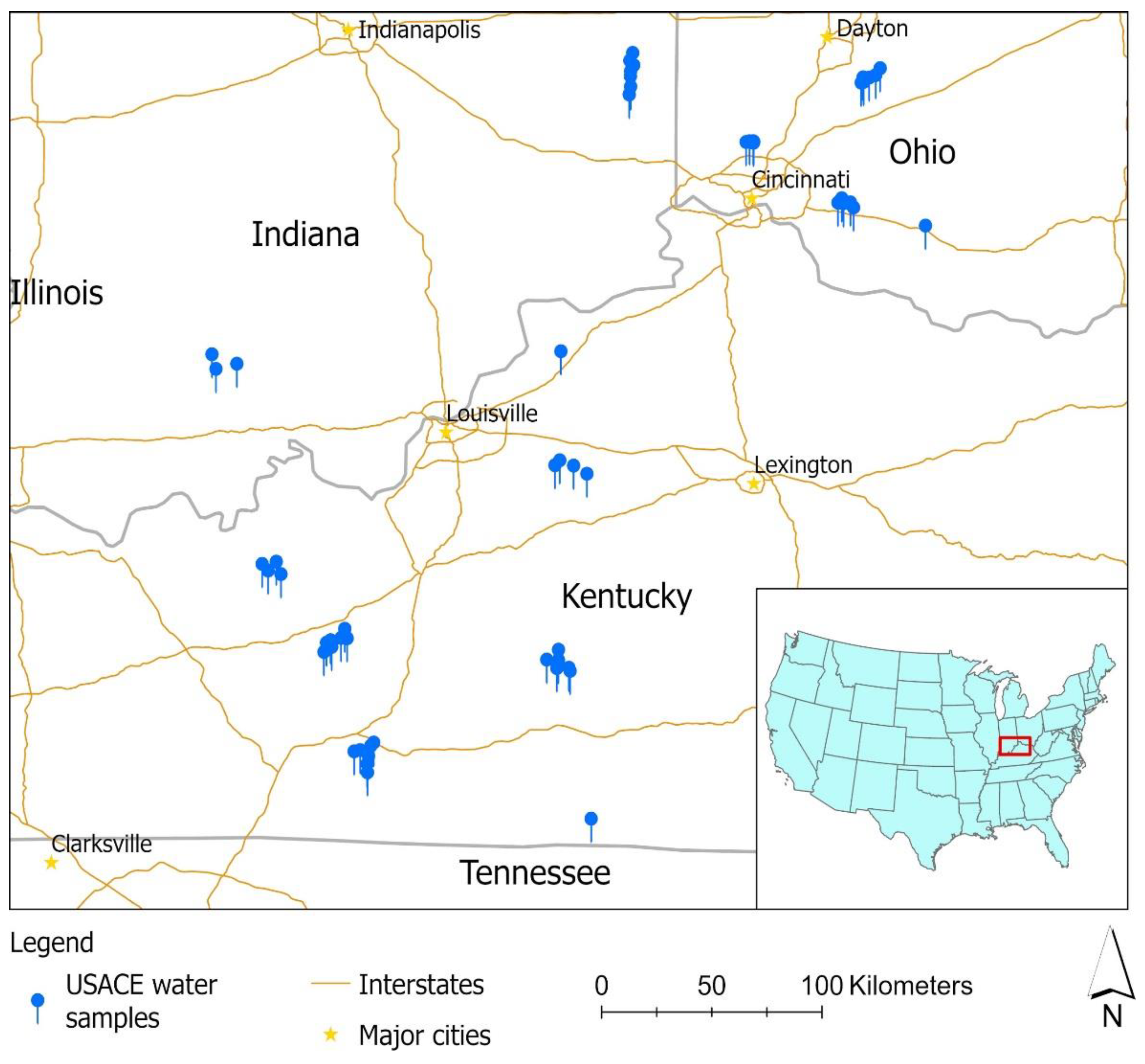
2. Study Area and Data

Figure 1 shows the extent of the study area and the locations of water quality samples obtained by the U.S. Army Corps of Engineers (USACE) Louisville District Water Quality Team [48]. In situ water quality data have been consistently collected for 12 USACE lakes in the tri-state region, including 5 in Kentucky (Barren River Lake, Green River Lake, Nolin River Lake, Rough River Lake, and Taylorsville Lake), 4 in Indiana (Brookville Lake, Cagles Mill Lake, Monroe Lake, and Patoka Lake), and 3 in Ohio (Caesar Creek Lake, West Fork Lake, and Harsha Lake) (https://www.lrl.usace.army.mil/Missions/CivilWorks/Water-Information/Water-Quality/). USACE water quality data provide in situ measurements of surface water temperature (°C), dissolved oxygen (milligrams per liter), pH, turbidity (nephelometric turbidity units (NTU)), Secchi depth (meter), and surface chlorophyll concentration (micrograms per liter). This water quality dataset covers the time period between May 2013 and November 2017. Chl-a concentration measurements are used in the present study for the development and validation of the SVM predictive models.
The USACE water quality data were collected in the months of May, June, July, August, September, and October. The Chl-a concentrations varied from 1.3 to 63.1 μg/L, with an average value of 9.9 μg/L and a standard deviation of 7.8 μg/L. There are seasonal changes in the mean values of the Chl-a samples, indicating the role of climate and some other seasonal factors such as agriculture activities in shaping Chl-a concentrations in these lakes. The average Chl-a values (μg/L) gradually increase from May (7.7) to June (8.2), July (8.4), August (9.1), and reach the peak in September (11.7). It then drops in October (8.4) to a similar level as in June and July.

3. Methods

3.1. Multi-Source Data Inquiry Implemented on Google Earth Engine

This study focused on multispectral satellite datasets available in GEE that correspond to the USACE water quality dataset for the Louisville region, including Landsat 7 and 8 and Sentinel-2A and 2B (Table 1). For remote sensing applications, the synchronization between ground sampling and satellite overpasses is important to ensure that the ground sample data and satellite images are from the same water quality status. At the developing stage of algal blooms, the water spectral characteristics could change within several days or even hours. Ideally, the water quality sampling can be planned in advance to take place on a cloud-free day coincident with satellite overpass. However, in reality, many water quality samples do not exactly match cloud-free satellite observations in time due to survey logistics constraints and the uncertainty of weather conditions. The use of multi-sensor images from a large number of satellites orbiting Earth greatly increases the opportunity to find cloud-free satellite observations for a given ground water quality sample survey.
The GEE satellite data repository and computing algorithms make it possible to automatically locate cloud-free image pixels that match the water quality samples in location and time. The search and inquiry script was written in Python based on the “geemap” package that wraps the GEE algorithms (https://github.com/giswqs/geemap). To ensure a sufficient number of match-up points for model development between the ground samples and satellites, a time window is allowed in the temporal matching. Namely, if no corresponding image pixels can be found on the same day of ground water quality data acquisition, the temporally closest image among those images within a time window of the water quality sampling date (i.e., 2 days) is acquired. Table 1 shows the availability of the major GEE satellite image assets and their bands corresponding to Landsat TM. A Python script was written to automatically search in the data archives with given date and coordinates (Figure S1). We examined cloud-free image vs. sample location/time searches using 2-day and 10-day time windows. A 2-day temporal window resulted in 38 match-up points with Landsat 8 images (05/2013–09/2017), 23 match-up points with Landsat 7 (05/2013–09/2017), 26 match-up points with Sentinel-2A (08/2016–09/2017), and 1 match-up point with Sentinel-2B (09/27/2017). No match-up points were found with Landsat-5 images for the time period in which water samples were acquired. Optical satellite images are often affected by clouds and hazes. A simple haze and cloud detection algorithm described in the next section was used to identify image pixels contaminated by clouds and hazes. After excluding these contaminated pixels (Figure 2), 56 match-up points were obtained for calibrating and evaluating the predictive model. If the temporal search window is expanded from 2 days to 10 days as in [48], all 97 USACE water samples have matching cloud-free image pixels. However, there is concern that the low synchronization between match-up points may not be adequate to support the model construction since water quality conditions can change significantly within 10 days. The use of the multi-sensor satellite image sources in GEE repository increases the number of match-up points for model development, but it is important to understand to what extent the inconsistency between different satellite sources affects the accuracy of the predictive model.

3.2. Cloud Masking and Haze Detection

Cloudy pixels were initially masked using the data quality assessment (QA) layer of each satellite data product to ensure that only cloud-free surface reflectance values were used to form match-up points. For example, Sentinel-2 surface reflectance Tier-1 product on GEE has a data layer “QA60” indicating the cloud condition. Those pixels that are indicated to be part of a cloud or cloud shadow are replaced with “NoData’’ or null. The cloud mask worked for most cloud conditions. However, it cannot detect haze caused by dust and air pollution or thin clouds. As illustrated in Figure 2, the haze did not block ground reflectance measurements of the satellite sensor but still contaminated the ground reflectance by adding path radiance from the haze to all bands. The haze effect is particularly detrimental for water quality mapping because of the low-albedo nature of water pixels. Therefore, a haze detection algorithm should be used to remove the pixels with serious haze contamination. Most haze/cloud detection algorithms, such as the Normalized Difference Vegetation Index (NDVI), Normalized Difference Snow Index (NDSI), Whiteness, and B4/B5 ratio [49], were developed for land features, and they are not suitable to detect the haze over water pixels. Our extensive experiments show that the blue band is most sensitive to the haze contamination and it is most likely to be contaminated if surface reflectance in the blue band is greater than 0.15. Therefore, we used a simple histogram slicing algorithm for haze detection and assigned a haze score of 0 for pixels with Rblue ≤ 0.15 and a haze score of 1.0 for pixels with Rblue > 0.15, where Rblue is the surface reflectance at the blue band.

3.3. GEE Surface Reflectance Data Validation

Removal of atmospheric interference is vital for water quality mapping because the majority of the total upwelling radiance over a water body received by the satellites originates from the atmospheric scattering [50,51]. The surface reflectance products in the GEE data repository were processed using different atmospheric correction algorithms. The Landsat 8 OLI images were corrected using the Land Surface Reflectance Code (LaSRC), which is a heritage of the MODIS and Landsat TM and ETM+ products [52]. To ensure the quality of satellite data, we compared the GEE OLI surface reflectance product against water surface reflectance collected by the ASD (Analytical Spectral Devices, Inc.) spectroradiometer in the field.
In total, 56 water samples on 21 September 2015 and 20 water samples on 9 October 2016 were collected with an ASD spectroradiometer in the wavelength range 350–1025 nm at 1 nm spectral resolution when Landsat 8 passed over Harsha Lake and Caesar Creek Lake in Ohio [46]. At each water sampling site, 40 spectral reflectance readings were collected by the ASD spectroradiometer and then processed to generate one representative reference spectrum. To evaluate the GEE Landsat 8 surface reflectance data, in situ ASD reference spectra collected at water sampling points were integrated to the five Landsat 8 bands (B1-B5) as ground references free of atmospheric influence, based on the Landsat 8 Spectral Response Functions (https://landsat.gsfc.nasa.gov/preliminary-spectral-response-of-the-operational-land-imager-in-band-band-average-relative-spectral-response/). Bands 6 and 7 of Landsat 8 images were not included because their wavelengths exceeded the ASD spectral range. The average RMS% (relative root mean square) was used as the criterion for quality assessment:
A v e r a g e   R M S %   = 100 i n ( R i ( A S D ) R i ( i m a g e ) ) 2 i n R i ( i m a g e ) 2
where Ri (ASD) is the in situ ASD reference reflectance for band i and Ri (image) is the reflectance in band i of the Landsat surface reflectance image.

3.4. Cross-Sensor Calibration between MSI and OLI over Water Bodies

In order to establish a cross-sensor calibration of at-surface reflectance for Sentinel-2 MSI and Landsat 8 OLI multispectral imagers, we examined their differences and then developed an empirical model to normalize them. The multispectral optical image products from Sentinel-2 MSI and Landsat 8 OLI were processed using different atmospheric correction algorithms. It was reported that the Sentinel-2 MSI level-2 surface reflectance product did not work well with the water quality data due to the algorithm used for atmospheric correction [48]. The Landsat 8 OLI images in GEE were corrected using the Land Surface Reflectance Code (LaSRC), which is a heritage of the MODIS and Landsat TM and ETM+ products [52]. In contrast, Sentinel-2 products used the Sentinel 2 Correction (Sen2Cor) algorithm. As shown in Figure 3, Landsat 7 ETM+ and Landsat 8 OLI images are statistically comparable and similar over water quality sample sites but are quite different from Sentinel-2 MSI surface reflectance values (Figure 3). As marked in Figure 3, the mean value of Landsat 8 OLI is 0.284, while the mean value of Sentinel-2 MSI is 0.969. The differences can be attributed to different band radiometric characteristics (0.48 vs. 0.49 um), spatial resolutions (30 vs. 10 m), and atmospheric correction algorithms (LaSRC vs. Sen2Cor). Therefore, direct use of the two surface reflectance products from Landsat and Sentinel-2 sensors without cross-sensor calibration may bias the predictive models.
To deal with the cross-sensor difference between these two products, the United States National Aeronautics and Space Administration (NASA) simulated the two instruments from hyperspectral data collected by the Hyperion instrument over 500 individual sites around the world and fitted linear equations to adjust the surface reflectance of each Sentinel-2 band to match the corresponding Landsat-8 band. NASA has released a consistently combined product for Landsat 8 and Sentinel-2 imagery [53,54]. Barsi et al. [55] used pseudo-invariant calibration sites (PICS) to calibrate an empirical equation to reconcile the cross-sensor differences between Sentinel-2 MSI top-of-atmosphere reflectance with Landsat 8 OLI. With a similar approach, we used a linear regression model to remove the systematic bias between Sentinel-2 MSI and Landsat 8 OLI images.
From the multi-sensor inquiry on GEE, overlapping Sentinel-2 MSI images and Landsat images (either OLI or ETM+) at 16 water sample sites were identified and used as radiometric tie points. After removal of one outlier from these radiometric tie points, a linear regression equation was fitted for each surface reflectance band (Figure 4). All regression equations were statistically significant, with coefficients of determination (R2) above 0.45. Bands 4 and 6 have slightly lower R2 values compared to other bands. Band 7 has the highest R2 value. Using these linear equations, the Sentinel-2 MSI surface reflectance values were converted and normalized to Landsat reflectance values and merged with other Landsat OLI or ETM+ samples for training the predictive model.

3.5. Machine Learning Model for Chl-a Mapping

Previously, various empirical models have been tested to map Chl-a concentrations [17,24,34,56,57]. Tebbs et al. [24] developed a linear regression model for mapping Chl-a in Lake Bogoria, Kenya, based on time-series Landsat ETM+ images and monthly in situ measurements of Chl-a for the period from November 2003 to February 2005. They found that the performance of their model was sensitive to the selection of bands or band ratio combinations. In general, blue to green spectral bands are better for estimating Chl-a concentrations in clear (oligotrophic) water conditions [16,58], while red and near-infrared bands are preferable in high-biomass and turbid coastal and inland waters [19,58,59]. The major criticism for the empirical regression models is that the assumption of a linear relationship between spectral reflectance and Chl-a may not hold for waters with a complicated optical condition, particularly for inland and coastal waters with relatively high biomass (Chl-a > 20 μg/L) [7].
Machine learning algorithms (e.g., support vector machines, neural networks, decision trees) have been increasingly used in mapping Chl-a in the past two decades, due to their robustness to image noise and lack of strong assumptions about data samples (e.g., normal distribution) [60,61,62,63,64,65,66]. Among machine learning algorithms, the support vector machine (SVM) method has its merit in requiring fewer samples because its learning power is determined by the data samples at cluster borders to define the “hyperplane” [67]. It has been demonstrated that the SVM has better performance than other machine learning models under small-sample scenarios [64,68]. In this case study, the 2-day search window resulted in a relatively small sample set consisting of 56 match-up points. Therefore, the SVM algorithm was selected as the predictive model because of its superior performance in a small-sample condition [68], which represents a major challenge for most water quality mapping projects.
The SVM regression model was set with a radial basis function (RBF) kernel using the R “e1071” package. All of the variables were standardized to avoid any bias caused by unit differences. The model parameters, cost and gamma, were fine-tuned using a genetic algorithm (GA) by setting the number of populations to be 50 and the number of generations to be 100. The crossover probability was set to 0.8, and the mutation probability was set to 0.1. The prediction accuracy of the fine-tuned SVM model was assessed using an independent validation dataset. The match-up points were randomly split into training and validation sets with 75% and 25% of all samples. The SVM model trained with the training set was assessed by the validation set. The root mean squared error (RMSE) and the mean absolute percentage error (MAPE) defined below were used to evaluate the model performance under different data scenarios.
R M S E = i = 1 n ( y i y i ^ ) 2 n
M A P E   = 100 % n i = 1 n | y i y i ^ y i |
where y i is the observed value and y i ^ is the predicted value. The model is calibrated by minimizing the RMSE of the training data. The minimization might overfit the model; that is, even though the RMSE of the training data is small, that of the validation data remains large. Therefore, both RMSEs of the training data and the validation data are reported.

3.6. Scenario Tests of the Multi-Sensor Approach with Different Search Windows

Xu et al. [69] used a much larger temporal window to form match-up points for constructing empirical models for predicting Chl-a concentration. For 97 water samples, Landsat 8 OLI images were manually searched to identify images closest in time to the samples. Even though radiometric calibration and atmospheric correction were carefully applied, the RMSE of the prediction model (6.17 μg/L) is higher than the result in this research. Xu et al. [69] only used one satellite sensor (Sentinel-2 MSI) to form match-up points for model construction. Because the search was constrained to a single sensor, the water samples and the paired satellite reflectance measurements may not capture the same water conditions.
Using multi-sensor data can shorten the temporal gap between satellite overpass and ground sampling. However, the sensor configurations and spectral responses of different sensors might introduce uncertainty to the data as well. Therefore, it is important to check which way might bring more uncertainty—adding more sensors or allowing for larger time gaps. To answer this question, we compared the model prediction performance under five different data scenarios (S#) composed by different sensor and search window combinations (Table 2):
S1: Use 97 match-up points that are formed by searching the readily available multi-sensor (OLI, ETM+, and MSI) surface reflectance products in GEE with a 10-day window to identify the paired image pixels for ground water samples.
S2: Use the 56 match-up points that are formed by only searching the OLI surface reflectance products in GEE with a 10-day window.
S3: Use the 56 match-up points that are formed by searching the multi-sensor (OLI, ETM+, and MSI) surface reflectance products in GEE with a 2-day window.
S4: Use the 32 match-up points that are formed by searching the OLI surface reflectance products in GEE with a time window between 2 days and 10 days from the corresponding ground sample dates.
S5: Use the 32 match-up points that are formed by searching the multi-sensor (OLI, ETM+, and MSI) surface reflectance products in GEE with a time window between 2 days and 10 days from the corresponding ground sample dates.
Among these data scenarios, S1 is the baseline scenario because it uses cross-sensor data and a comparable time window with Xu et al. [69]. The comparisons between S2 and S3 and between S4 and S5 scenarios show the effect of sensor differences on the performance of the prediction model, and the comparisons between S2 and S4 and between S3 and S5 show the effect of larger time gaps (> 2 days but up to 10 days) for pairing match-up points on the model performance. These scenario studies are helpful to answer the research questions of the paper.

4. Results

4.1. Surface Reflectance Validation

The datasets on GEE were provided as a bulk. Therefore, there might be some uncertainty in the data products, which could affect the model prediction of Chl-a. The uncertainty of some images used in this research was measured by using the field data collected from a spectrometer. The averaged RMS% was computed for each spectral band from field sampling points (Table 3). Among the 20 sampling sites across the lake, half of them have a turbidity value close to 0 NTU and, at those sites, GEE Landsat 8 reflectance data generated extremely large average RMS% values at bands 1–5, which were 84.17%, 70.07%, 56.85%, 52.97%, and 61.23%, respectively. If excluding these sites, the GEE Landsat 8 reflectance at the remaining sites matches well with the in situ ASD reflectance measurements at bands 1–4, with average RMS% less than 25%, as shown in Table 3. This indicates that the GEE Landsat 8 reflectance data could be problematic for the water quality monitoring of very clear waters. Harmful algal blooms frequently occur on Harsha Lake. GEE Landsat 8 reflectance at sampling sites of Harsha Lake yielded average RMS% less than 30% at bands 2–4. In both cases, the quality of GEE Landsat 8 reflectance data (bands 1–4) is acceptable. In particular, reflectance at bands 2–4 is often more accurate than reflectance at band 1, and band 5 reflectance is the least accurate, indicated by the very large average RMS% (greater than 60%).
Atmospheric correction over the water surface is particularly more difficult than other land cover types because of the low signal-to-noise ratio of satellite images over water bodies. The validation of the OLI surface reflectance product using ASD surface reflectance indicates that the quality of Landsat 8 OLI surface reflectance data from GEE is sufficient for modeling Chl-a. These results show the necessity of normalizing Sentinel-2 MSI to Landsat 7 ETM+ and Landsat 8 OLI surface reflectance using the cross-sensor calibration.

4.2. SVM Model Performance under Different Data Scenarios

The SVM model parameters and accuracy reports under the five data scenarios discussed in the Methods section (Table 2) are listed in Table 4 below. The following facts can be observed from the table.
First, the SVM model accuracy under scenario S1 is better than that reported in [69]. For the match-up point formation, scenario S1 uses the same length of temporal search window (10 days) as in [64]. S1 uses the GEE image assets to find the paired image pixels, instead of conducting user-specified atmospheric corrections as in [64]. In addition, S1 used multiple sensors for finding the best match-up points. This result indicates that the direct use of GEE image assets can skip atmospheric correction-related image preprocessing tasks and make it much more convenient to establish the prediction model for multi-site and multi-date Chl-a mapping. The multi-sensor approach reduces the time gaps between the ground samples and satellite overpassing and therefore improves the data quality for training the predictive models. At the same time, the use of an SVM machine learning model may have contributed to the prediction accuracy improvement. It is worth noting that S1 has the lowest MAPE value, indicating that even if it does not produce the smallest RMSE, it has the best accuracy relative to the magnitude and variance of Chl-a. Especially, the RMSEs of the training and validation datasets are similar in S1, which suggests that the model was not overfitted.
Second, S3 has lower RMSE and MAPE than S2. These two scenarios have the same number of samples. S3 used the multi-sensor search, while S2 only searched OLI images. This indicates that the reduction in temporal gaps between ground samples and satellite observations for the paired match-up points by using the multi-sensor approach improved the predictive model performance.
Third, the overfitting problem is present in S2-S5, but not in S1. The overfitting problem is indicated by the significantly larger RMSE value for the validation than that for the training set (Table 4). The overfitting problem may be caused by the small number of match-up points in S2–S5 (less than 60), although our use of the GA algorithm in assisting SVM parameter calibration mitigates the overfitting. It is worth noting the water samples used in this research were collected before Sentinel-2 satellites were launched in March 2017. It is expected that the chance of pairing future ground samples with satellite data could be greatly improved by the constellation of Sentinel-2 satellites.
Lastly, in S1, all ground water samples are paired with cloud-free multi-sensor satellite observations within the 10-day window, and 97 match-up points are formed for the model development. Although the quality of match-up points could be compromised by the larger temporal time window, the model prediction accuracy in S1 is still the best among the data scenarios. This result suggests that it is a valid option to use a large temporal window (e.g., 10 days) to ensure a sufficient number of match-up points (e.g., > 80) for the prediction model development when the match-up rate of the ground samples is low, at the same time using multi-sensor data to minimize the time gaps. In short, S1 provides enough training and evaluation match-ups for our SVM/GA algorithm to effectively map Chl-a concentrations at a regional scale with reasonable accuracy in this study.

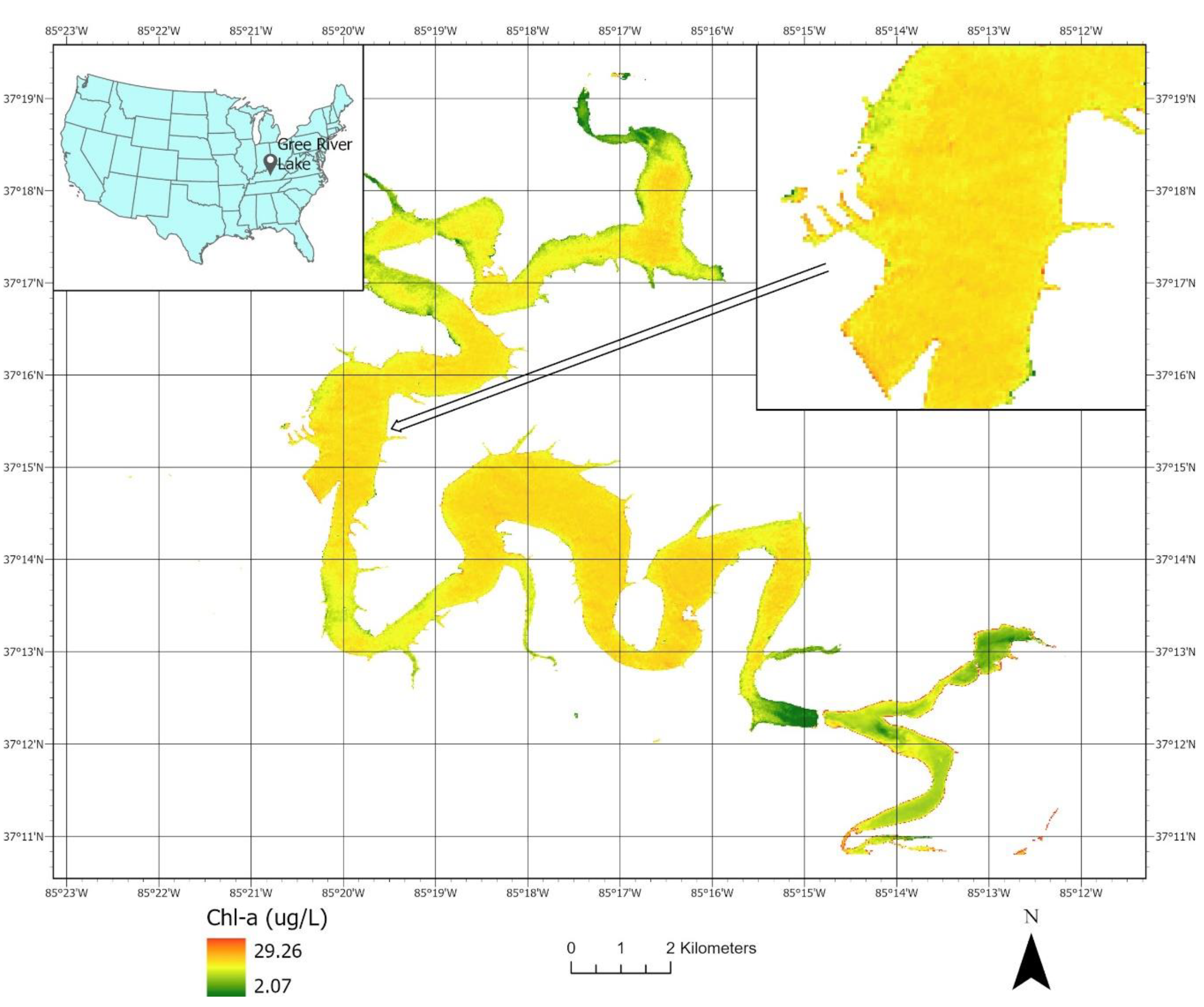
4.3. Predicting Chl-a in an Unsampled Lake within the Study Area

The SVM model was trained using the sample data to predict Chl-a concentration in the study area with the images obtained from the GEE image repositories. One of the unsampled lakes, Green River Lake in Kentucky, is displayed in Figure 5 to show the predicted Chl-a concentration from a Sentinel-2A image acquired on 28 August 2016. The map shows a spatially coherent distribution of Chl-a concentration in the lake. Such spatial coherence is expected and follows the First Law of Geography [70] regarding the quality of spatial data.

5. Discussion

5.1. Comparison with Other Studies

Recent research by Zhang et al. [71] applied an SVM model with an RBF kernel on Landsat 8 OLI images to estimate the chlorophyll-a concentrations of multiple lakes in China. Their 90 match-up samples were formed using Landsat OLI images acquired on two cloud-free days, respectively, in December 2017 and in March 2018, over five lakes. Water samples acquired on the exact same days of two Landsat OLI overpasses were used to form their match-up points, and six spectral bands were used in the model construction. They reported an RMSE of 22.636 μg/L. Although we have a similar number of samples and the similar SVM with an RBF kernel to theirs, the RMSE of our SVM model (4.424 μg/L) is considerably smaller than theirs. The high absolute RMSE in Zhang et al. can be attributed to the “extremely high” Chl-a concentration (over 200 μg/L) in some lakes of their study area. In a water quality assessment project in the U.S., Xu et al. [69] manually corrected Landsat 8 OLI images for calibrating empirical models with the same set of water samples as in our study, and they reported a comparable RMSE of 6.17 μg/L. Therefore, our model evaluation shows that the quality of GEE public data assets is sufficient for mapping freshwater Chl-a in a large geographical region. In other words, the readily available surface reflectance products in the GEE repository can be used for large-scale water quality mapping applications, and users do not have to go through the complicated atmospheric correction of raw image products on their own. The direct use of GEE satellite data products for water quality applications not only saves a lot of image processing time associated with atmospheric correction but also makes the model predictions reproducible and comparable and makes effective and routine water quality monitoring feasible and affordable. Cross-sensor calibration is still necessary, but it does not add much complexity if the linear regression in Section 3.4 is used.

5.2. Chl-a Sample Data Variability with Various Time Intervals

We conducted some tests of the change in Chl-a samples with different time windows using the sites sampled on multiple dates in the same year. The sampling time intervals include 1, 2, 3, 28, 30, 39, 40, 48, 49, 55, 58, or 67 days based on the USACE reference data. The average change in Chl-a (μg/L) and percentage of change are displayed in Table 5.
The sampling interval up to three days had little impact (less than 10%) on the sample values. However, when the interval was too long (30 days), the percent difference could be as large as 42.3%. Unfortunately, our samples did not have the 10-day interval measurement, and therefore the data could not show the impact of the 10-day interval on the Chl-a samples. The data scenario S1 used the 10-day window to search the multi-sensor datasets, and the accuracy was the highest among all scenarios. This indicates that a 10-day window is a valid option if the number of samples is too low.

6. Summary and Conclusions

Google Earth Engine (GEE) provides data repositories and scripting tools for users to conduct cloud-based image processing and inquiry. Mapping Chl-a in freshwater lakes often faces the challenge of a small number of samples that can be paired with satellite images. This research demonstrates a workable solution to maximize match-up points by searching cloud-free and haze-free image pixels from the GEE data repositories using online scripts. The support vector machine (SVM) model trained using the match-up points, consisting of ground water quality samples paired with GEE image pixels returned from the inquiries, can predict Chl-a concentration with reasonable accuracy. The major findings are summarized below:
  • Google Earth Engine greatly facilitates the pairing of satellite surface reflectance image pixels with corresponding field water quality samples to form match-up points for predictive model development. The cloud-based inquiry supported by GEE makes it much more efficient to use Landsat 7 ETM+ for land resource mapping. In our case, we found 22 match-up points by pairing Landsat 7 ETM+ pixels with the water quality samples, which was around one-third of the 56 match-up points used for training the SVM model.
  • The RMSE of Chl-a of the SVM model trained by the data obtained from single-source (OLI only) imagery was 4.42 μg/L (compared with 6.17 μg/L in a previous project report using the same sample data). It is evident that the GEE image product is reliable for water quality mapping.
  • A smaller temporal search window (two-day window) for pairing field water samples with the multi-sensor satellite images in GEE data repositories improves the model prediction accuracy, but the improvement is not significant and reduces the number of match-up training and validation sample/image pixel pairs, which introduces model overfitting.
  • The use of multi-sensor image data from GEE improves the data match-up between ground samples and satellite images and therefore improves the model prediction accuracy.
  • For mapping water quality parameters over a multistate region, the number of match-up points needs to be large enough to avoid the model overfitting bias. In our case, the number of match-up points from three states and 12 lakes should be in the order of 90 to avoid overfitting. Models with less than 60 match-up points may suffer from the overfitting problem.
Overall, GEE with reflectance normalization between satellites and sufficient water quality sample data in combination with our new SVM/GA model results in an effective, affordable, and feasible satellite water quality monitoring system for inland waters at regional scales. This research can serve as a case study and example for future water quality mapping using GEE. It is worth noting that although Landsat 5 TM surface reflectance was not included in the experiments of this research, it remains comparable with Landsat 7 ETM+, Landsat 8 OLI, and Sentinel-2A and B. A slight modification of the Python codes developed in this research will allow similar queries to be performed on Landsat 5 TM datasets.

Supplementary Materials

The following are available online at https://0-www-mdpi-com.brum.beds.ac.uk/2072-4292/12/20/3278/s1, Figure S1: Python script for automatic search.

Author Contributions

Conceptualization, L.W., H.L., and Q.W.; methodology, L.W.; software, L.W. and Q.W.; validation, L.W. and M.X.; formal analysis, L.W. and M.X.; investigation, L.W. and M.X.; resources, L.W., Q.W., and M.X.; data curation, L.W. and M.X.; writing—original draft preparation, L.W.; writing—review and editing, L.W., H.L., M.X., Q.W., R.B., M.R., E.E., J.Y., and Y.L.; visualization, L.W.; supervision, L.W.; project administration, L.W., H.L., and R.B.; funding acquisition, L.W. All authors have read and agreed to the published version of the manuscript.

Funding

This research received no external funding.

Acknowledgments

This research received no external funding. The work was supported by the scholarships of HSS Manship Summer Research Fellowship and LSU Libraries Open Access Author Fund of Louisiana State University. The authors thank the editor and the anonymous reviewers for their constructive comments that have helped improve the content and presentation of this paper.

Conflicts of Interest

The authors declare no conflict of interest.

References

  1. Lunetta, R.S.; Schaeffer, B.A.; Stumpf, R.P.; Keith, D.; Jacobs, S.A.; Murphy, M.S. Evaluation of cyanobacteria cell count detection derived from MERIS imagery across the eastern USA. Remote Sens. Environ. 2015, 157, 24–34. [Google Scholar] [CrossRef]
  2. Trevino-Garrison, I.; DeMent, J.; Ahmed, F.S.; Haines-Lieber, P.; Langer, T.; Ménager, H.; Neff, J.; Van der Merwe, D.; Carney, E. Human Illnesses and Animal Deaths Associated with Freshwater Harmful Algal Blooms—Kansas. Toxins 2015, 7, 353–366. [Google Scholar] [CrossRef] [PubMed] [Green Version]
  3. Burford, M.A.; Carey, C.C.; Hamilton, D.P.; Huisman, J.; Paerl, H.W.; Wood, S.A.; Wulff, A. Perspective: Advancing the research agenda for improving understanding of cyanobacteria in a future of global change. Harmful Algae 2020, 91, 101601. [Google Scholar] [CrossRef] [PubMed]
  4. Ho, J.C.; Michalak, A.M. Exploring temperature and precipitation impacts on harmful algal blooms across continental U.S. lakes. Limnol. Oceanogr. 2020, 65, 992–1009. [Google Scholar] [CrossRef] [Green Version]
  5. Matthews, M.W.; Bernard, S.; Winter, K. Remote sensing of cyanobacteria-dominant algal blooms and water quality parameters in Zeekoevlei, a small hypertrophic lake, using MERIS. Remote Sens. Environ. 2010, 114, 2070–2087. [Google Scholar] [CrossRef]
  6. De Figueiredo, D.R.; Azeiteiro, U.M.; Esteves, S.M.; Gonçalves, F.J.M.; Pereira, M.J. Microcystin-producing blooms--a serious global public health issue. Ecotoxicol. Environ. Saf. 2004, 59, 151–163. [Google Scholar] [CrossRef]
  7. Matthews, M.W.; Bernard, S.; Robertson, L. An algorithm for detecting trophic status (chlorophyll-a), cyanobacterial-dominance, surface scums and floating vegetation in inland and coastal waters. Remote Sens. Environ. 2012, 124, 637–652. [Google Scholar] [CrossRef]
  8. Backer, L.C. Cyanobacterial Harmful Algal Blooms (CyanoHABs): Developing a Public Health Response. Lake Reserv. Manag. 2002, 18, 20–31. [Google Scholar] [CrossRef]
  9. Francy, D.S.; Graham, J.L.; Stelzer, E.A.; Ecker, C.D.; Brady, A.M.G.; Struffolino, P.; Loftin, K.A. Water Quality, Cyanobacteria, and Environmental Factors and Their Relations to Microcystin Concentrations for Use in Predictive Models at Ohio Lake Erie and Inland Lake Recreational Sites, 2013–14; Scientific Investigations Report 2015-5120; U.S. Geological Survey: Columbus, OH, USA, 2015. [CrossRef] [Green Version]
  10. Mishra, D.R.; Ogashawara, I.; Gitelson, A.A. Bio-Optical Modeling and Remote Sensing of Inland Waters; Elsevier: Amsterdam, The Netherlands, 2017; ISBN 9780128046548. [Google Scholar] [CrossRef]
  11. Hong, Z.; Li, X.; Han, Y.; Zhang, Y.; Wang, J.; Zhou, R.; Hu, K. Automatic sub-pixel coastline extraction based on spectral mixture analysis using EO-1 Hyperion data. Front. Earth Sci. 2019, 13, 478–494. [Google Scholar] [CrossRef]
  12. Agha, R.; Cirés, S.; Wörmer, L.; Domínguez, J.A.; Quesada, A. Multi-scale strategies for the monitoring of freshwater cyanobacteria: Reducing the sources of uncertainty. Water Res. 2012, 46, 3043–3053. [Google Scholar] [CrossRef]
  13. Wynne, T.T.; Stumpf, R.P.; Tomlinson, M.C.; Warner, R.A.; Tester, P.A.; Dyble, J.; Fahnenstiel, G.L. Relating spectral shape to cyanobacterial blooms in the Laurentian Great Lakes. Int. J. Remote Sens. 2008, 29, 3665–3672. [Google Scholar] [CrossRef]
  14. Matthews, M.W.; Odermatt, D. Improved algorithm for routine monitoring of cyanobacteria and eutrophication in inland and near-coastal waters. Remote Sens. Environ. 2015, 156, 374–382. [Google Scholar] [CrossRef]
  15. Kutser, T.; Hedley, J.; Giardino, C.; Roelfsema, C.; Brando, V.E. Remote sensing of shallow waters—A 50 year retrospective and future directions. Remote Sens. Environ. 2020, 240, 111619. [Google Scholar] [CrossRef]
  16. Kutser, T. Passive optical remote sensing of cyanobacteria and other intense phytoplankton blooms in coastal and inland waters. Int. J. Remote Sens. 2009, 30, 4401–4425. [Google Scholar] [CrossRef]
  17. Mishra, S.; Mishra, D.R. A novel remote sensing algorithm to quantify phycocyanin in cyanobacterial algal blooms. Environ. Res. Lett. 2014, 9, 114003. [Google Scholar] [CrossRef]
  18. Duan, H.; Ma, R.; Hu, C. Evaluation of remote sensing algorithms for cyanobacterial pigment retrievals during spring bloom formation in several lakes of East China. Remote Sens. Environ. 2012, 126, 126–135. [Google Scholar] [CrossRef]
  19. Jupp, D.L.B.; Kirk, J.T.O.; Harris, G.P. Detection, identification and mapping of cyanobacteria—Using remote sensing to measure the optical quality of turbid inland waters. Mar. Freshw. Res. 1994, 45, 801–828. [Google Scholar] [CrossRef]
  20. Sòria-Perpinyà, X.; Vicente, E.; Urrego, P.; Pereira-Sandoval, M.; Ruíz-Verdú, A.; Delegido, J.; Soria, J.M.; Moreno, J. Remote sensing of cyanobacterial blooms in a hypertrophic lagoon (Albufera of València, Eastern Iberian Peninsula) using multitemporal Sentinel-2 images. Sci. Total Environ. 2020, 698, 134305. [Google Scholar] [CrossRef]
  21. Mchau, G.J.; Makule, E.; Machunda, R.; Gong, Y.Y.; Kimanya, M. Phycocyanin as a proxy for algal blooms in surface waters: Case study of Ukerewe Island, Tanzania. Water Pract. Technol. 2019, 14, 229–239. [Google Scholar] [CrossRef]
  22. Wei, G.; Tang, D.; Wang, S. Distribution of chlorophyll and harmful algal blooms (HABs): A review on space based studies in the coastal environments of Chinese marginal seas. Adv. Space Res. 2008, 41, 12–19. [Google Scholar] [CrossRef]
  23. Caballero, I.; Fernández, R.; Escalante, O.M.; Mamán, L.; Navarro, G. New capabilities of Sentinel-2A/B satellites combined with in situ data for monitoring small harmful algal blooms in complex coastal waters. Sci. Rep. 2020, 10, 8743. [Google Scholar] [CrossRef] [PubMed]
  24. Tebbs, E.J.; Remedios, J.J.; Harper, D.M. Remote sensing of chlorophyll-a as a measure of cyanobacterial biomass in Lake Bogoria, a hypertrophic, saline–alkaline, flamingo lake, using Landsat ETM+. Remote Sens. Environ. 2013, 135, 92–106. [Google Scholar] [CrossRef]
  25. Han, L.; Jordan, K.J. Estimating and mapping chlorophyll-a concentration in Pensacola Bay, Florida using Landsat ETM data. Int. J. Remote Sens. 2005, 26, 5245–5254. [Google Scholar] [CrossRef]
  26. Borup, M.B.; Brett Borup, M.; Narteh, V.N.A. Mapping and Modeling Chlorophyll-a Concentration in Utah Lake Using Landsat 7 ETM Imagery. Proc. Water Environ. Fed. 2013, 2013, 1251–1257. [Google Scholar] [CrossRef]
  27. Oyama, Y.; Matsushita, B.; Fukushima, T. Distinguishing surface cyanobacterial blooms and aquatic macrophytes using Landsat/TM and ETM shortwave infrared bands. Remote Sens. Environ. 2015, 157, 35–47. [Google Scholar] [CrossRef]
  28. Taufik, M.; Wiliyanto, N. Chlorophyll-a Spread Analysis Using Meris And Aqua Modis Satellite Imagery (Case Study: Coastal Waters of Banyuwangi). Geoid 2016, 11, 198. [Google Scholar] [CrossRef]
  29. Ali, K.A.; Ortiz, J.D. Multivariate approach for chlorophyll-a and suspended matter retrievals in Case II type waters using hyperspectral data. Hydrol. Sci. J. 2016, 61, 200–213. [Google Scholar] [CrossRef]
  30. Zolfaghari, K.; Duguay, C. Estimation of Water Quality Parameters in Lake Erie from MERIS Using Linear Mixed Effect Models. Remote Sens. 2016, 8, 473. [Google Scholar] [CrossRef] [Green Version]
  31. Kudela, R.M.; Palacios, S.L.; Austerberry, D.C.; Accorsi, E.K.; Guild, L.S.; Torres-Perez, J. Application of hyperspectral remote sensing to cyanobacterial blooms in inland waters. Remote Sens. Environ. 2015, 167, 196–205. [Google Scholar] [CrossRef] [Green Version]
  32. Hunter, P.D.; Tyler, A.N.; Carvalho, L.; Codd, G.A.; Maberly, S.C. Hyperspectral remote sensing of cyanobacterial pigments as indicators for cell populations and toxins in eutrophic lakes. Remote Sens. Environ. 2010, 114, 2705–2718. [Google Scholar] [CrossRef] [Green Version]
  33. Rivera-Caicedo, J.P.; Verrelst, J.; Muñoz-Marí, J.; Camps-Valls, G.; Moreno, J. Hyperspectral dimensionality reduction for biophysical variable statistical retrieval. ISPRS J. Photogramm. Remote Sens. 2017, 132, 88–101. [Google Scholar] [CrossRef]
  34. Vincent, R.K.; Qin, X.; McKay, R.M.L.; Miner, J.; Czajkowski, K.; Savino, J.; Bridgeman, T. Phycocyanin detection from LANDSAT TM data for mapping cyanobacterial blooms in Lake Erie. Remote Sens. Environ. 2004, 89, 381–392. [Google Scholar] [CrossRef]
  35. Ma, R.; Dai, J. Investigation of chlorophyll-a and total suspended matter concentrations using Landsat ETM and field spectral measurement in Taihu Lake, China. Int. J. Remote Sens. 2005, 26, 2779–2795. [Google Scholar] [CrossRef]
  36. Modiegi, M.; Rampedi, I.T.; Tesfamichael, S.G. Comparison of multi-source satellite data for quantifying water quality parameters in a mining environment. J. Hydrol. 2020, 591, 125322. [Google Scholar] [CrossRef]
  37. Mushtaq, F.; Nee Lala, M.G. Remote estimation of water quality parameters of Himalayan lake (Kashmir) using Landsat 8 OLI imagery. Geocarto Int. 2017, 32, 274–285. [Google Scholar] [CrossRef]
  38. Gorelick, N.; Hancher, M.; Dixon, M.; Ilyushchenko, S.; Thau, D.; Moore, R. Google Earth Engine: Planetary-scale geospatial analysis for everyone. Remote Sens. Environ. 2017, 202, 18–27. [Google Scholar] [CrossRef]
  39. Kumar, L.; Mutanga, O. Google Earth Engine Applications Since Inception: Usage, Trends, and Potential. Remote Sens. 2018, 10, 1509. [Google Scholar] [CrossRef] [Green Version]
  40. Wang, C.; Jia, M.; Chen, N.; Wang, W. Long-Term Surface Water Dynamics Analysis Based on Landsat Imagery and the Google Earth Engine Platform: A Case Study in the Middle Yangtze River Basin. Remote Sens. 2018, 10, 1635. [Google Scholar] [CrossRef] [Green Version]
  41. Gujrati, A.; Jha, V.B. Surface water dynamics of inland water bodies of india using google earth engine. ISPRS Ann. Photogramm. Remote Sens. Spat. Inf. Sci. 2018, 4, 467–472. [Google Scholar] [CrossRef] [Green Version]
  42. Murphy, S.; Wright, R.; Rouwet, D. Color and temperature of the crater lakes at Kelimutu volcano through time. Bull. Volcanol. 2018, 80. [Google Scholar] [CrossRef]
  43. Markert, K.; Schmidt, C.; Griffin, R.; Flores, A.; Poortinga, A.; Saah, D.; Muench, R.; Clinton, N.; Chishtie, F.; Kityuttachai, K.; et al. Historical and Operational Monitoring of Surface Sediments in the Lower Mekong Basin Using Landsat and Google Earth Engine Cloud Computing. Remote Sens. 2018, 10, 909. [Google Scholar] [CrossRef] [Green Version]
  44. Griffin, C.G.; McClelland, J.W.; Frey, K.E.; Fiske, G.; Holmes, R.M. Quantifying CDOM and DOC in major Arctic rivers during ice-free conditions using Landsat TM and ETM data. Remote Sens. Environ. 2018, 209, 395–409. [Google Scholar] [CrossRef]
  45. Kuhn, C.; de Matos Valerio, A.; Ward, N.; Loken, L.; Sawakuchi, H.O.; Kampel, M.; Richey, J.; Stadler, P.; Crawford, J.; Striegl, R.; et al. Performance of Landsat-8 and Sentinel-2 surface reflectance products for river remote sensing retrievals of chlorophyll-a and turbidity. Remote Sens. Environ. 2019, 224, 104–118. [Google Scholar] [CrossRef] [Green Version]
  46. Jia, T.; Zhang, X.; Dong, R. Long-Term Spatial and Temporal Monitoring of Cyanobacteria Blooms Using MODIS on Google Earth Engine: A Case Study in Taihu Lake. Remote Sens. 2019, 11, 2269. [Google Scholar] [CrossRef] [Green Version]
  47. Weber, S.J.; Mishra, D.R.; Wilde, S.B.; Kramer, E. Risks for cyanobacterial harmful algal blooms due to land management and climate interactions. Sci. Total Environ. 2020, 703, 134608. [Google Scholar] [CrossRef]
  48. Xu, M.; Liu, H.; Beck, R.; Lekki, J.; Yang, B.; Shu, S.; Liu, Y.; Benko, T.; Anderson, R.; Tokars, R.; et al. Regionally and Locally Adaptive Models for Retrieving Chlorophyll-a Concentration in Inland Waters From Remotely Sensed Multispectral and Hyperspectral Imagery. IEEE Trans. Geosci. Remote Sens. 2019, 57, 4758–4774. [Google Scholar] [CrossRef]
  49. Zhu, Z.; Woodcock, C.E. Object-based cloud and cloud shadow detection in Landsat imagery. Remote Sens. Environ. 2012, 118, 83–94. [Google Scholar] [CrossRef]
  50. Bernstein, L.S.; Jin, X.; Gregor, B.; Adler-Golden, S.M. Quick atmospheric correction code: Algorithm description and recent upgrades. Organ. Ethic. 2012, 51, 111719. [Google Scholar] [CrossRef]
  51. Gao, B.-C.; Montes, M.J.; Davis, C.O.; Goetz, A.F.H. Atmospheric correction algorithms for hyperspectral remote sensing data of land and ocean. Remote Sens. Environ. 2009, 113, S17–S24. [Google Scholar] [CrossRef]
  52. Vermote, E.; Justice, C.; Claverie, M.; Franch, B. Preliminary analysis of the performance of the Landsat 8/OLI land surface reflectance product. Remote Sens. Environ. 2016, 185, 46–56. [Google Scholar] [CrossRef]
  53. Claverie, M.; Ju, J.; Masek, J.G.; Dungan, J.L.; Vermote, E.F.; Roger, J.-C.; Skakun, S.V.; Justice, C. The Harmonized Landsat and Sentinel-2 surface reflectance data set. Remote Sens. Environ. 2018, 219, 145–161. [Google Scholar] [CrossRef]
  54. Flood, N. Comparing Sentinel-2A and Landsat 7 and 8 Using Surface Reflectance over Australia. Remote Sens. 2017, 9, 659. [Google Scholar] [CrossRef] [Green Version]
  55. Barsi, J.A.; Alhammoud, B.; Czapla-Myers, J.; Gascon, F.; Haque, M.O.; Kaewmanee, M.; Leigh, L.; Markham, B.L. Sentinel-2A MSI and Landsat-8 OLI radiometric cross comparison over desert sites. Eur. J. Remote Sens. 2018, 51, 822–837. [Google Scholar] [CrossRef]
  56. Schalles, J.F.; Yacobi, Y.Z. Remote detection and seasonal patterns of phycocyanin, carotenoid and chlorophyll pigments in eutrophic waters. Ergebnisse Der Limnologie 2000, 55, 153–168. [Google Scholar]
  57. Randolph, K.; Wilson, J.; Tedesco, L.; Li, L.; Pascual, D.L.; Soyeux, E. Hyperspectral remote sensing of cyanobacteria in turbid productive water using optically active pigments, chlorophyll a and phycocyanin. Remote Sens. Environ. 2008, 112, 4009–4019. [Google Scholar] [CrossRef]
  58. Moses, W.J.; Gitelson, A.A.; Berdnikov, S.; Povazhnyy, V. Corrections to “Satellite Estimation of Chlorophyll-a Concentration Using the Red and NIR Bands of MERIS—The Azov Sea Case Study”. IEEE Geosci. Remote Sens. Lett. 2009, 6, 876. [Google Scholar] [CrossRef]
  59. Darecki, M.; Stramski, D. An evaluation of MODIS and SeaWiFS bio-optical algorithms in the Baltic Sea. Remote Sens. Environ. 2004, 89, 326–350. [Google Scholar] [CrossRef]
  60. Atkins, J.P.; Burdon, D.; Allen, J.H. An application of contingent valuation and decision tree analysis to water quality improvements. Mar. Pollut. Bull. 2007, 55, 591–602. [Google Scholar] [CrossRef]
  61. Schiller, H.; Doerffer, R. Neural network for emulation of an inverse model operational derivation of Case II water properties from MERIS data. Int. J. Remote Sens. 1999, 20, 1735–1746. [Google Scholar] [CrossRef]
  62. Huang, W.G.; Lou, X.L. AVHRR detection of red tides with neural networks. Int. J. Remote Sens. 2003, 24, 1991–1996. [Google Scholar] [CrossRef]
  63. Chen, Q.; Mynett, A.E. Predicting Phaeocystis globosa bloom in Dutch coastal waters by decision trees and nonlinear piecewise regression. Ecol. Modell. 2004, 176, 277–290. [Google Scholar] [CrossRef]
  64. Xie, Z.; Lou, I.; Ung, W.K.; Mok, K.M. Freshwater Algal Bloom Prediction by Support Vector Machine in Macau Storage Reservoirs. Math. Probl. Eng. 2012, 2012. [Google Scholar] [CrossRef]
  65. Lee, S.; Lee, D. Four Major South Korea’s Rivers Using Deep Learning Models. Int. J. Environ. Res. Public Health 2018, 15, 1322. [Google Scholar] [CrossRef] [PubMed] [Green Version]
  66. Kumar, A.C.; Bhandarkar, S.M. A deep learning paradigm for detection of harmful algal blooms. In Proceedings of the 2017 IEEE Winter Conference on Applications of Computer Vision (WACV), Santa Rosa, CA, USA, 24–31 March 2017; pp. 743–751. [Google Scholar]
  67. Cortes, C.; Vapnik, V. Support-vector networks. Mach. Learn. 1995, 20, 273–297. [Google Scholar] [CrossRef]
  68. Wang, L.; Liu, H.; Su, H.; Wang, J. Bathymetry retrieval from optical images with spatially distributed support vector machines. GIScience Remote Sens. 2019, 56, 323–337. [Google Scholar] [CrossRef]
  69. Xu, M.; Liu, H.; Beck, R.A.; Reif, M.; Young, J.L. Regional Analysis of Lake and Reservoir Water Quality with Multispectral Satellite Remote Sensing Images; ERDC: Vicksburg, MS, USA, 2019. [Google Scholar]
  70. Tobler, W. On the First Law of Geography: A Reply. Ann. Assoc. Am. Geogr. 2004, 94, 304–310. [Google Scholar] [CrossRef]
  71. Zhang, T.; Huang, M.; Wang, Z. Estimation of chlorophyll-a Concentration of lakes based on SVM algorithm and Landsat 8 OLI images. Environ. Sci. Pollut. Res. Int. 2020, 27, 14977–14990. [Google Scholar] [CrossRef]
Figure 1. Study area: blue pins are the water samples collected by the USACE Louisville District Water Quality Team from May 2013 to November 2017.
Remotesensing 12 03278 g001
Figure 2. A good quality image pixel of Landsat 8 OLI (left) on 05/01/2013 and a poor quality Landsat 7 ETM+ (right) on 05/02/2013 with haze contamination matched with the ground samples at the Jericho Lake, Kentucky. The lower panels show the spectral profiles of the pixels marked in the two images.
Remotesensing 12 03278 g002
Figure 3. Frequency distributions of surface reflectance over water quality samples from (a) Sentinel-2 MSI, (b) Landsat 8 OLI, and (c) Landsat 7 ETM+.
Remotesensing 12 03278 g003
Figure 4. Band calibration between Sentinel-2 MSI (x-axis) and Landsat 8 OLI (y-axis) surface reflectance: (a) Band 1; (b) Band 2; (c) Band 3; (d) Band 4; (e) Band 5; (f) Band 7. (Note: the x axis and the y axis of the charts mark the reflectance values multiplied by 10,000). For consistency, the band names refer to the Thematic Mapper bands.
Remotesensing 12 03278 g004
Figure 5. Predicted Chl-a concentration of the Green River Lake, Kentucky with a Sentinel-2 (Scene ID: L1C_T16SFG_A009904_20170515T163103) overpass on 28 August 2016.
Remotesensing 12 03278 g005
Table 1. List of major multispectral satellite data assets on GEE and their band signations compatible with Thematic Mapper (TM).
Satellite
Sensor
Surface Reflectance
Product Availability
Optical Bands
Landsat 5 TMMarch 1984–May 2012TM1, TM2, TM3, TM4, TM5, TM7
Landsat 7 ETM+January 1999–PresentB1(TM1), B2(TM2), B3(TM3), B4(TM4), B5(TM5), B7(TM7)
Landsat 8 OLIApril 2013–PresentB2(TM1), B3(TM2), B4(TM3), B5(TM4), B6(TM5), B7(TM7)
Sentinel-2 MSIMarch 2017–PresentB2(TM1), B3(TM2), B4(TM3), B8A((TM4), B11(TM5), B12(TM7)
Terra ASTERMarch 2000–Present
(Top-Of-Atmosphere
radiance only)
B1(TM2), B2(TM3), B3N(TM4), B6(TM5)
Table 2. Testing scenarios with different search time windows and multi-sensor configurations.
Data ScenariosTime Window (Days)Sensor(s)Number of Samples
S110OLI, ETM+, and MSI97
S210OLI only56
S32OLI, ETM+, and MSI56
S42–10OLI only32
S52–10OLI, ETM+, and MSI32
Table 3. Average RMS% of the GEE Landsat 8 reflectance data in comparison with ASD samples.
Average RMS%B1B2B3B4B5
Caesar Creek Lake22.78%19.98%23.11%15.26%64.82%
Harsha Lake35.15%26.75%27.30%27.73%68.44%
Table 4. Parameters and accuracies of the SVM models under the five data scenarios.
Data ScenariosSVM Parameters
from GA Calibration
RMSE Training
Data (μg/L)
RMSE Validation
Data (μg/L)
MAPE
Validation Data
S1cost = 5.589
gamma = 0.045
7.5044.42434.17%
S2cost = 9.928
gamma = 1.348
0.7755.80757.42%
S3 cost = 8.979
gamma = 1.995
0.7784.98548.53%
S4cost = 3.521
gamma = 0.445
1.3653.56244.98%
S5cost = 9.790
gamma = 0.277
1.0144.03551.19%
Table 5. Chl-a change in different time windows.
Time Window (Days)Chl-a Change (μg/L)Chl-a Change (%)
31.112.2%
303.642.3%
405.1122.8%
504.340.2%
>504.046.2%

