Retrieval of Sea Surface Wind Speed from Spaceborne SAR over the Arctic Marginal Ice Zone with a Neural Network


1
Key Laboratory of Digital Earth Science, Aerospace Information Research Institute, Chinese Academy of Sciences, Beijing 100094, China
2
GuangXi Vocational College of Safety Engineering, NanNing 530100, China
3
University of Chinese Academy of Sciences, Beijing 100049, China
*
Author to whom correspondence should be addressed.
Remote Sens. 2020, 12(20), 3291; https://0-doi-org.brum.beds.ac.uk/10.3390/rs12203291
Submission received: 8 August 2020
/
Revised: 26 September 2020
/
Accepted: 2 October 2020
/
Published: 10 October 2020
(This article belongs to the Special Issue Synthetic Aperture Radar Observations of Marine Coastal Environments)
Abstract
:In this paper, we presented a method for retrieving sea surface wind speed (SSWS) from Sentinel-1 synthetic aperture radar (SAR) horizontal-horizontal (HH) polarization data in extra-wide (EW) swath mode, which have been extensively acquired over the Arctic for polar monitoring. In contrast to the conventional algorithm, i.e., using a geophysical model function (GMF) to retrieve SSWS by spaceborne SAR, we introduced an alternative retrieval method based on a GMF-guided neural network. The SAR normalized radar cross section, incidence angle, and wind direction are used as the inputs of a back propagation (BP) neural network, and the output is the SSWS. The network is developed based on 11,431 HH-polarized EW images acquired in the marginal ice zone (MIZ) of the Arctic from 2015 to 2018 and their collocated scatterometer wind measurements. Verification of the neural network based on the testing dataset yields a bias of 0.23 m/s and a root mean square error (RMSE) of 1.25 m/s compared to the scatterometer wind data for wind speeds less than approximately 30 m/s. Further comparison of the SAR retrieved SSWS with independent buoy measurements shows a bias and RMSE of 0.12 m/s and 1.42 m/s, respectively. We also analyzed the uncertainty of the retrieval when reanalysis model wind direction data are used as inputs to the neural network. By combining the detected sea ice cover information based on SAR data, sea ice and marine-meteorological parameters can be derived simultaneously by spaceborne SAR at a high spatial resolution in the Arctic.

1. Introduction
The retrieval of sea surface wind by spaceborne synthetic aperture radar (SAR) has been studied for a few decades. The most common retrieval method adopts a geophysical model function (GMF), which was originally designed for a microwave scatterometer to retrieve sea surface wind fields. A GMF generally has the following format:
The above GMF empirically relates the normalized radar cross section (NRCS, ) with the wind speed at a 10 m reference height , azimuthal wind direction and incidence angle θ through various linear or nonlinear functions of , and . p is a constant. Different GMFs for C-band radar (often called CMOD) data with vertical-vertical (VV) polarization have been proposed and are widely exploited to acquire sea surface wind fields at a high spatial resolution, e.g., from the CMOD4, CMOD5, and CMOD5.N to the currently used CMOD7 [1,2,3,4,5] and CMOD_IFR2 [6]. On the other hand, as spaceborne SAR can also operate in horizontal-horizontal (HH) polarization, the so-called polarization ratio (PR) can be used to transform the HH-polarized NRCS into the VV-polarized NRCS; then the GMFs developed for VV-polarized data can be applied to retrieve the sea surface wind fields. However, the dependence of PR is not only on incidence angles [7,8,9], but also on wind conditions [8,10]. In addition to using the PR models, one can develop independent GMFs dedicated for HH-polarized spaceborne SAR data, e.g., as proposed in [11] for the Radarsat data and in [12] for Environmental Satellite (ENVISAT)/advanced synthetic aperture radar (ASAR) data in HH polarization. Developing independent GMF should be an optimized method to retrieve wind fields with spaceborne SAR data in HH polarization, as the PR may depend on various factors through nonlinear relations.
When spaceborne SAR satellites operating at different microwave frequencies from C-band are in orbit, the functions in (1) must be refined to make them suitable for retrieving sea surface wind fields, e.g., the LMOD [13] for the L-band Advanced Land Observing Satellite (ALOS)/Phased Array L-band synthetic aperture radar (PALSAR) and the XMOD [14] for the X-band TerraSAR-X and TanDEM-X. Although the format of (1) is compact, the functions , , and are complicated; they often consist of sub-functions and generally, more than 30 coefficients need to be determined. Moreover, to the best of our knowledge, the formats of these functions are empirically fitted to a large amount of tuning data.
Sentinel-1A (S1A) and Sentinel-1B (S1B) were launched in 2014 and 2016, respectively. These twin satellites have extensively acquired the extra-wide (EW) swath data with a polarization combination of HH and horizontal-vertical (HV) for sea ice monitoring in the Arctic. Of particular note is the marginal ice zone (MIZ), generally defined as the transition area between sea ice and open water, where the sea ice concentration is between 15% and 80%. With the rapid decline of sea ice in the Arctic, its seasonal MIZ is widening [15], which leads to significant interactions between sea ice and ocean dynamics. Therefore, to support scientific research, resource utilization, and navigation safety, we intend to derive sea surface winds at a high spatial resolution from these EW data acquired in the Arctic, in combination with sea ice information.
We preliminarily analyzed combinations of CMOD5.N with different PR models for retrieving sea surface wind speed (denoted SSWS hereafter) by using S1 HH-polarized data [16]. The retrievals were compared with in situ buoy data and scatterometer wind data. As most of the S1 acquisitions over buoys are in VV polarization (which features the best response to the sea surface), only 130 scenes of the S1 data in HH polarization were acquired from October 2014 to December 2018 over the National Data Buoy Center (NDBC) buoys. Table 1 summarizes the comparisons using different PR modes with CMOD5.N, as well as using the CMODH [12].
Machine learning algorithms have demonstrated great potential for the mining of information from ocean remote sensing data (e.g., as reviewed in [17]), and they generally have a strong capability of fitting the nonlinear curves, e.g., the one represented by (1). As described above, tuning the GMFs for spaceborne SAR data is challenging because multiple non-linear functions and sub-functions need to be empirically or statistically determined. With the acquisitions of a large amount of S1 data, it would be interesting to investigate the retrievals of marine-meteorological parameters by spaceborne SAR data based on machine learning algorithms. Therefore, in this paper, we present a method for retrieving SSWS from S1 EW data in HH polarization based on a neural network.
Following the introduction, the datasets used are listed in Section 2. Section 3 describes the method of constructing a back propagation (BP) neural network to retrieve SSWS from S1 data in HH polarization. We verified the trained BP neural network by comparing the retrievals with the ASCAT data. Then, we further validated the retrievals by comparing them with in situ buoy measurements and measurements from the Chinese icebreaker XueLong in the Arctic. These comparisons are presented in Section 4. The discussion and summary are given in the last two sections.
2. Datasets
2.1. S1 Data Acquired in the Arctic
The majority of the S1 data acquired over the Arctic are in the EW and interferometric wide (IW) swath modes. EW mode data have been extensively acquired throughout the Arctic (approximately 2500 images per month), since the S1A and S1B have formed the constellation in 2016. The EW mode data acquired in the Arctic are generally in the polarization combination of HH and HV. In this study, the EW mode data in HH polarization are used for retrieval of sea surface wind, as HH-polarized data have a more sensitive response to the sea surface than HV-polarized data. EW mode data have a swath width of approximately 400 km and the incidence angles vary between 18.9° and 47.0° from the near range to far range. The pixel size of EW data is 40 m × 40 m in both the azimuth and range directions.
2.2. ASCAT Wind Data
ASCAT is a spaceborne C-band (5.255 GHz) scatterometer that was launched on the European Organization for the Exploitation of Meteorological Satellites (EUMETSAT) MetOp-A satellite in October 2006. Another ASCAT instrument became operational on MetOp-B upon being launched in September 2012. ASCAT uses a vertically polarized antenna, whose primary objective is to obtain wind vectors over the global ocean.
Daily EUMETSAT ASCAT-A/B sea surface wind data under all weather conditions with a spatial resolution of 0.25° × 0.25° were collected in this study. These data were spatially and temporally collocated with the S1 data acquired in the MIZ of the Arctic, which is described in detail in the next section.
2.3. In Situ Data
In the present study, 289 S1 images acquired in EW and IW modes in HH polarization from October 2014 to October 2019 were collected and matched with data from 41 NDBC buoys. As S1 data in VV polarization are generally acquired over buoys, considerably fewer S1 data in HH polarization are available over NDBC buoys. The detailed information of the used NDBC buoys is listed in the Table 2.
The ten-minute sea wind measurements of the buoys are used in the following analysis. As the anemometers mounted on the buoys are at different heights above sea surface, the measured wind speed data are converted to that at a 10 m reference height above the sea surface, which is described in detail in the next section.
In particular, we also collected in situ measurements of ocean winds acquired by the icebreaker XueLong in the Arctic to validate the retrieved S1 SSWS. The anemometer mounted on XueLong is at a height of 20 m above the sea surface.
3. Methodology
3.1. Collocation of S1 Data with ASCAT Data
The EW data were subjected to radiometric calibration and the removal of thermal noise according to the S1 user manual [18], referring to the Appendix A for details.
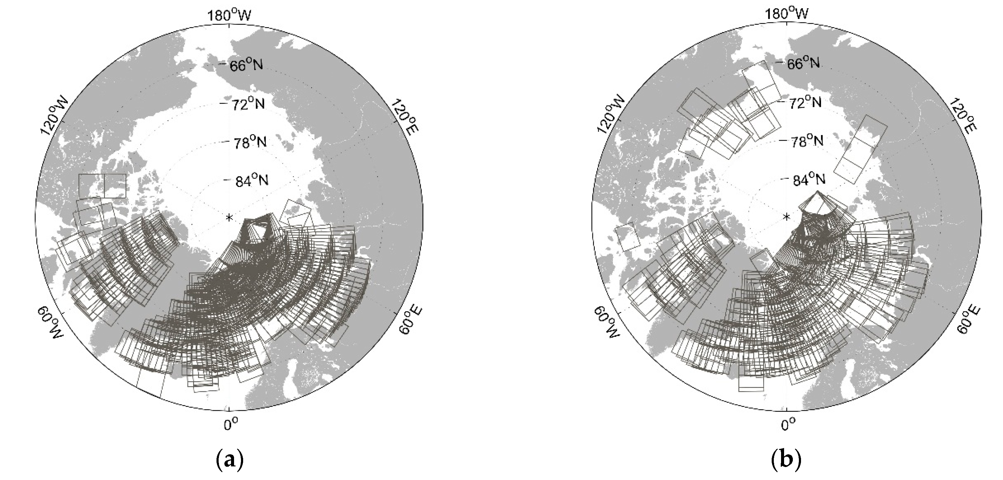
The S1 EW data in the Arctic MIZ from 2015 to 2018 were spatially and temporally collocated with ASCAT wind data with a spatial distance of less than 25 km and a temporal window of less than 60 min, respectively, which yields a total of 11,431 scenes of S1 EW images. Among the collocations, 8452 and 2979 SAR images were acquired by S1A and S1B, respectively. The spatial distributions of these collocated S1 images are shown in Figure 1. Evidently, the majority of the collocations are in the Atlantic sector of the Arctic.
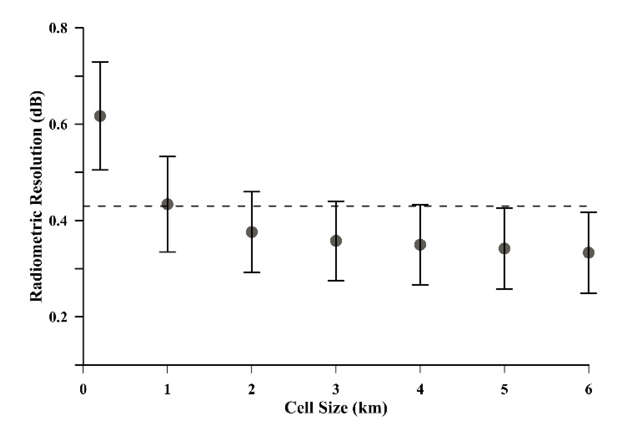
The inevitable existence of speckle noise in SAR images makes it impossible to retrieve sea surface wind fields at the primary pixel resolution. Therefore, the general procedure to reduce speckle noise in the SAR data is to spatially average the intensities of numbers of pixels to obtain a “cell”. Then, these cells, which represent the mean intensity of pixels, are used for retrieval of SSWS. Generally, the larger the cell size is, the better its radiometric resolution (denoted by , as defined in (2)), which is used to describe speckle noise [19].
where is the equivalent number of looks, given as follows:
where is the intensities of pixels in a cell, and and are the variance and mean of , respectively [20].
We sampled the 11,431 S1 EW images to different cells with sizes ranging from 200 m to 6 km, and the corresponding derived radiometric resolution (using (2)) is shown in Figure 2. The diagram suggests that the radiometric resolution decreases as the cell size increases. The decreasing magnitude trend is particularly evident for cell sizes smaller than 2 km. For example, given a cell size of 1 × 1 km, the mean radiometric resolution is 0.43 dB, which is equal to the absolute calibration accuracy of the S1 data of 0.43 dB [21] (marked by the dashed line in Figure 2). However, by taking account into the standard deviation (0.10 dB) of these data, the corresponding radiometric resolution varies between 0.53 and 0.33 dB. For comparison, the mean radiometric resolution of the data with a cell size of 2 × 2 km is 0.37 dB (and the standard deviation is 0.08 dB), which is lower than the absolute calibration accuracy of the S1 data. For cell sizes larger than 2 × 2 km, the decreasing trend of the radiometric resolution remains gentle. For instance, the radiometric resolution changes only from 0.36 to 0.33 dB, corresponding to the cell sizes changing from 3 × 3 km to 6 × 6 km. We expect to retrieve the sea surface wind field from SAR data at a high spatial resolution (i.e., using a small cell size for the retrievals). Therefore, to balance the trade−off between the radiometric resolution and spatial resolution of the retrieved SSWS, we chose a cell size of 2 × 2 km for the retrievals.
As some S1 EW data contain a mixture of sea ice and open water, the ice−covered sub−images are filtered out using the ice mapping system (IMS) reanalysis data [22]. We checked these data in another sea ice detection study based on S1 EW data [23], and they generally show consistency with the visual inspection of sea ice cover.
Further, open water sub−images are screened out using a homogeneity factor (described in the Appendix A), which has been widely applied for screening SAR data [24,25,26] containing features that make the sea surface inhomogeneous, e.g., targets, dark patterns (oil, upwelling, etc.), as well as sea ice. These two preprocessing steps ensure that the remaining SAR sub−images are suitable for the retrieval of SSWS.
Note that the determined S1 cell size (i.e., the sub−image size) is 2 × 2 km, while the ASCAT wind cell size is of 0.25° × 0.25°. Therefore, all the S1 sub−images collocated within an ASCAT wind cell were further averaged to obtain the mean NRCS.
Finally, after the processes described above, the 11,431 S1 images yield a total of 1,740,509 data pairs collocated with ASCAT wind data.
3.2. Collocation of S1 Data with in situ Data
As the in−situ wind data obtained by buoys and XueLong were used to validate the S1 retrieved SSWS, only the S1 acquisitions covering the locations of the NDBC buoys and the icebreaker were selected to minimize the uncertainty in the spatial collocation between the S1 data and in situ measurements. On the other hand, the ten−minute sea wind measurements were used. Therefore, the temporal interval between the in−situ measurements and S1 acquisitions should have a limited impact on the validation.
Each S1 sub−image with a size of 2 × 2 km where the buoy or XueLong located was extracted to conduct retrievals of SSWS and compare with the in−situ measurements. Accordingly, the 289 S1 images acquired in EW and IW modes in HH polarization from October 2014 to October 2019 were collocated with the 41 NDBC buoy data, yielding a total of 305 data pairs (indicating one S1 image that may have been matched up with more than one buoy).
All the measurements of wind speed () by anemometers mounted on buoys or on the icebreaker at different heights () above the sea surface were adjusted to the wind speed () at a 10 m reference height () using (4), assuming neutral wind conditions [27], for a comparison with the SAR retrievals:
where is the roughness length with a value of m.
Following the introduced methods for preparing the collocated datasets, the development of a GMF−guided BP neural network to retrieve SSWS by the S1 EW data is described in the following subsection.
3.3. Establishing and Training the BP Neural Network
The well−studied GMF presented in (1) suggests that the retrieval of the sea surface wind field from the radar NRCS follows a nonlinear relationship. Although the BP neural network, a traditional machine learning algorithm, was proposed a few decades ago [28], it forms the basis of modern neural networks in machine learning and is good at fitting such nonlinear curves.
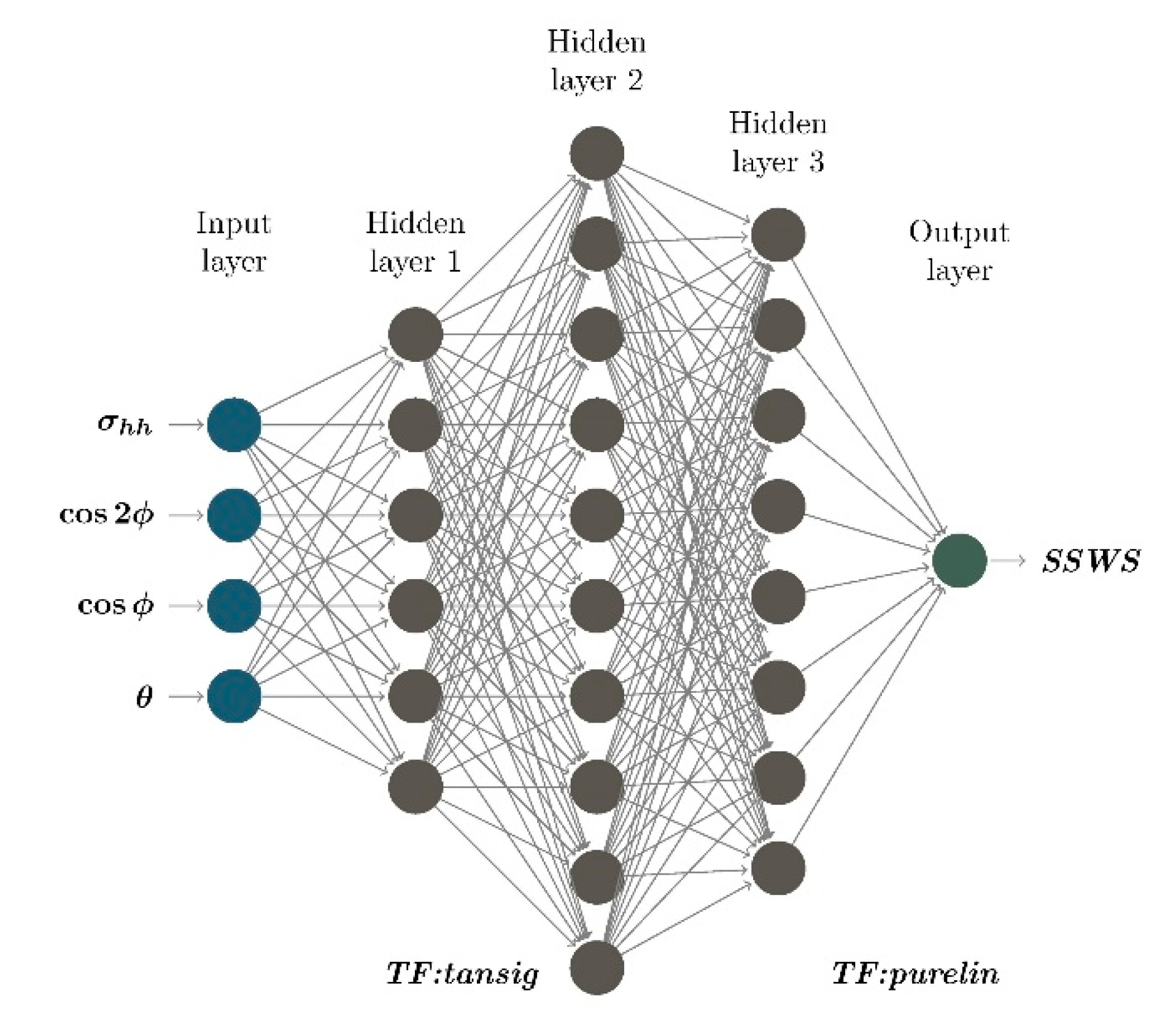
The designed BP network consists of an input layer, an output layer and three hidden layers, as illustrated in Figure 3. The numbers of nodes in the three hidden layers are 6, 10, and 8, respectively. Each neuron connects with all the neurons in the next layer, but there is no connection between neurons within the same layer.
Based on the expression of the general GMF (referring to (1)), there are four nodes in the input layer of the BP neural network: . is the averaged radar backscatter of the S1 sub−images, is the local incidence angle and is the azimuthal wind direction, i.e., the angle between the collocated ASCAT wind direction and S1 radar look direction.
The output layer node of the network has only one value of SSWS. The transfer function (abbreviated ‘TF’ in Figure 3) of the hidden layer is “tansig” (tangent S−type transfer function), which can converge quickly. The output layer transfer function is “purelin” (linear transfer function), which can make the network output arbitrary values. The training function is “traindx” (momentum BP algorithm with a variable learning rate), which has the fastest convergence speed for a medium−scale BP network. The learning function of the network is “learngdm” (gradient descent momentum learning function), which is used to calculate the change rate of weights and thresholds. The performance function of the network is the mean square error (MSE), which is a fast way to measure the “average error”.
Because of the difference among the magnitudes of values, either the network will not converge or the convergence speed will be very slow. Therefore, before training the network, the input values of and the output value of SSWS of the model are normalized according to the following equation:
where represents the input or output data, and are the maximum and minimum values, respectively, of the input or output data, and is the normalized input or output. After normalizing the data, we can train the network using the designed neural network model. Notably, the retrieved needs to be anti−normalized after training.
Figure 4 presents histograms of collocated ASCAT wind speeds and wind directions. The distribution of collocated wind directions is generally regular over 360 degrees, indicating that they can cover various conditions (from crosswind to upwind conditions, which yield the lowest and highest radar backscatter of sea surface, respectively). However, the distribution of wind speed is close to the Rayleigh distribution, in which high wind speeds (e.g., those higher than 15 m/s) are greatly reduced. Note that cases of wind speeds higher than approximately 22 m/s do exist in the collocated dataset, but they are barely visible in the histogram shown in Figure 4a as they account for a very small proportion of the whole dataset. Such an unbalanced training dataset can have a significant impact on the performance of the BP network. The training of a BP network ends according to whether the overall MSE between the outputs and the true values is less than a set threshold. Therefore, the use of training data that are limited at high wind speeds means that such data are taken into account less by the BP network when it tries to fit a nonlinear relationship among and based on a dataset whose majority are between 2 m/s and 15 m/s.
We used a somewhat “tricky” method to solve this problem. We first randomly chose 80% of the data with wind speeds lower than 4 m/s, 40% of the data with wind speeds between 4 m/s and 15 m/s, and 80% of the data with wind speeds higher than 15 m/s, which yielded a “pool” of training dataset (822,949 data pairs), denoted . As the distribution of collocated wind speeds is highly irregular, the proportions of data with different wind speeds for the training dataset were chosen to balance the different wind speeds. Then, we arbitrarily adjusted these data by duplicating cases of high wind speeds and discarding cases of low to moderate wind speeds, whose histogram roughly fits a normal distribution, as shown by the dark gray bars in Figure 4a. This resulted in another training dataset (762,350 data pairs), denoted .
The training of the neural network was terminated when it met the requirements of MSE (less than 0.001) or when training was performed for 50,000 iterations.
4. Results and Analysis
In this section, we first verify the trained network using both the training and the testing datasets. Comparisons of the S1 retrieved SSWS with the in−situ buoy data and the measurements from the icebreaker XueLong during its Arctic surveys in the summer season of 2017–2019 are also conducted.
4.1. Verification of the Training BP Network for SSWS Retrieval
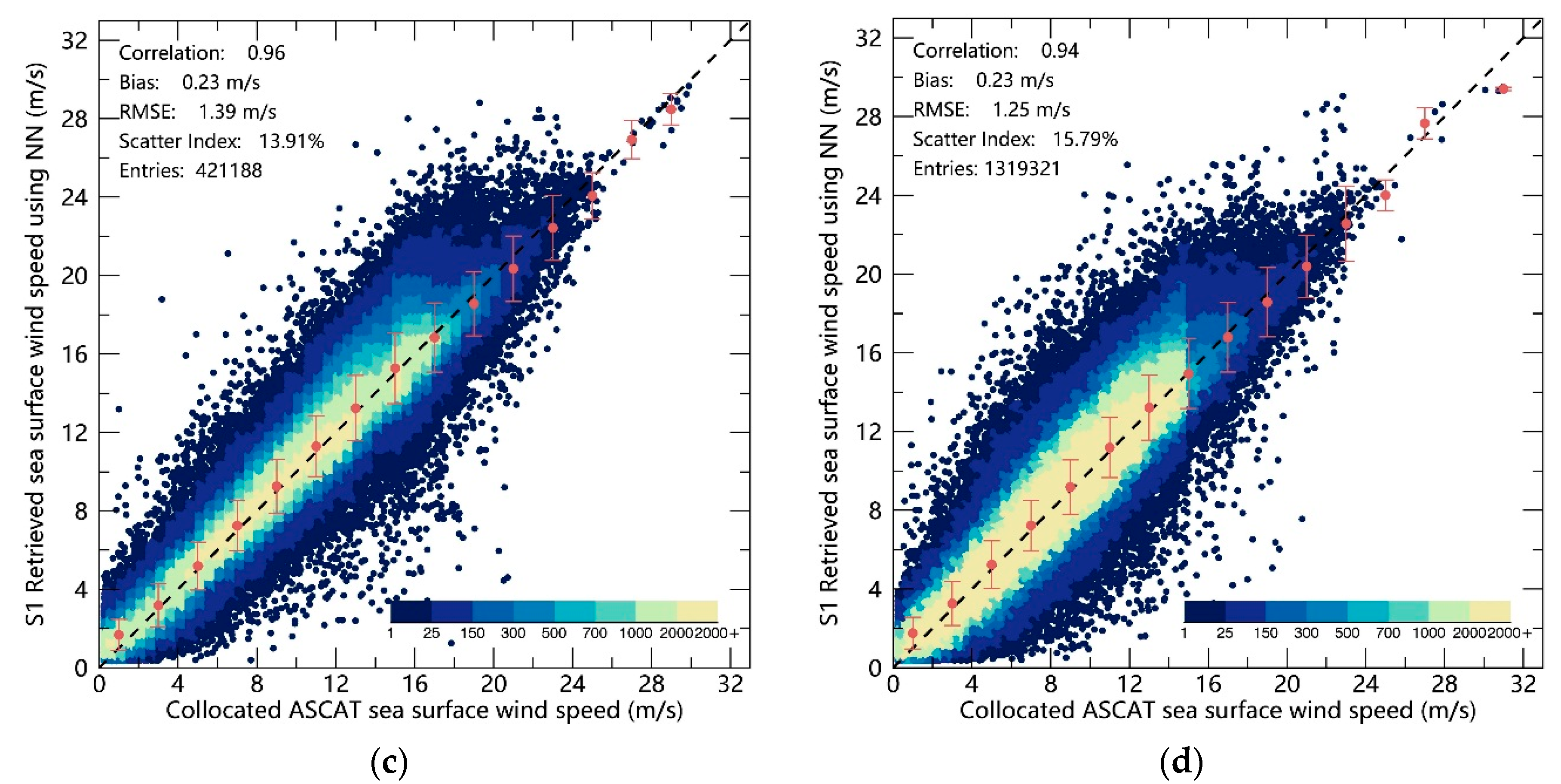
Figure 5 shows the comparisons between the retrieved SSWS and the collocated ASCAT wind speed based on the training and testing datasets.
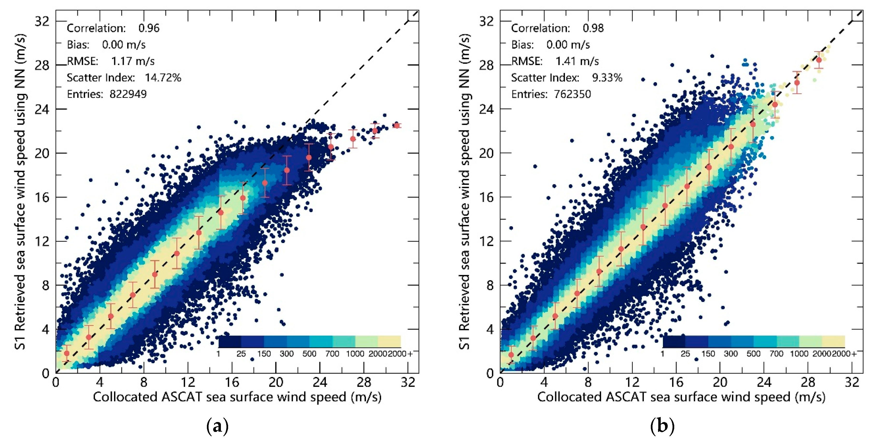
Figure 5a: Verification of the training result of the trial using the directly to train the neural network. The training yields a zero bias. However, the saturation of the S1 retrieved SSWS at approximately 24 m/s is distinctive. Unfortunately, the saturation problem cannot be solved even if all the high wind cases in the collocated data pairs were used to train the neural network.
Figure 5b: Verification of the training result of another trial using to train the neural network. Although the root mean square error (RMSE) increases slightly from 1.17 m/s to 1.45 m/s, the S.I. reduces significantly from 14.72% to 9.33%, comparing Figure 5a with 5b. More importantly, the bias shows very limited dependence on SSWS (referring to the overlaid error bars), and the saturation phenomenon does not appear, at least up to the highest SSWS of the collocated data pairs, approximately 32 m/s. This result suggests that the duplication of high wind cases functions in the BP neural network.
Figure 5c: Verification of the training result using to train the neural network, while excluding the duplicated high wind cases of the from the verification. The most distinct change when comparing (c) to (b) is that the bias increases from zero to 0.23 m/s. This is not surprising, as one can see that the amount of data pairs in (c) is only approximately 55% of that in (b), while the training of the neural network seeks an overall minimum bias.
Figure 5d: Verification of the training result achieved in (b) by using the testing data. The testing data consists of two parts. The first part is the remaining of full collocated dataset after selecting the original training dataset , i.e., 20% of the data with wind speeds lower than 4 m/s, 60% of the data with wind speeds between 4 m/s and 15 m/s, and 20% of the data with wind speeds higher than 15 m/s. The second part comprises the collocated data that belong to but are not within . Note that the remaining data that are not used for training the neural network are not regularly distributed in terms of their wind speed ranges; therefore, the data density in (d) does not change continuously. Comparing the verification results using the testing data and training data (Figure 5b), the bias increases to 0.23 m/s, which indicates that the overall SAR retrievals are higher than the ASCAT wind speeds, whereas the RMSE reduces slightly from 1.41 m/s to 1.25 m/s. On the other hand, the verification using the testing dataset shows that the bias in different wind speed ranges remains stable and the saturation is not observed.
Consequently, the trained neural network (i.e., the corresponding verification presented in Figure 5b) is used to retrieve SSWS from the S1 HH−polarized data, and the retrievals are further validated by comparing them with in situ measurements.
4.2. Comparison of the S1−Retrieved SSWS with in situ Measurements
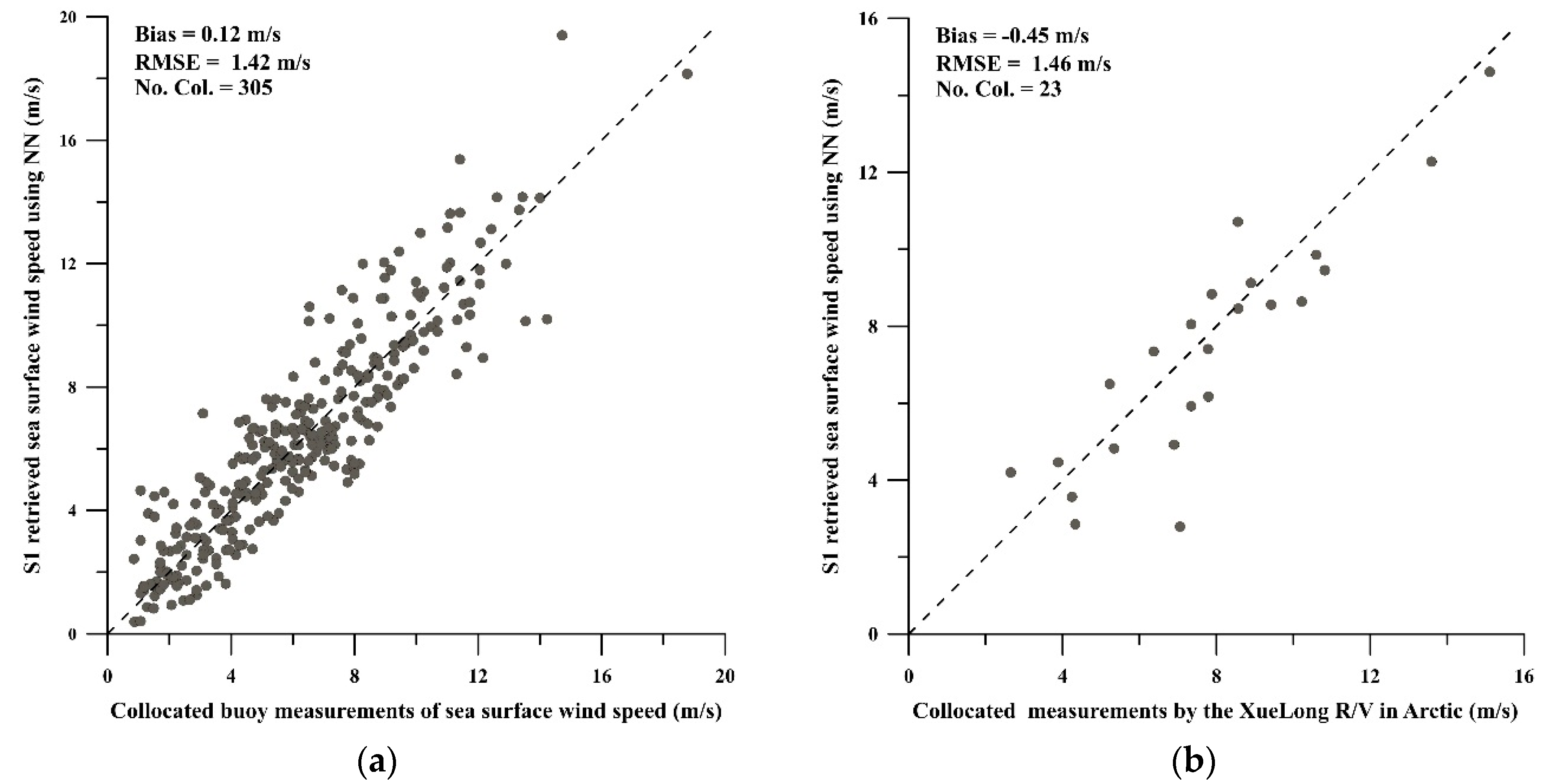
The diagram shown in Figure 6a presents the comparison of the S1−retrieved SSWS based on the BP neural network described above with the NDBC buoy measurements.
The comparison with the buoy measurements has a bias of 0.12 m/s and an RMSE of 1.42 m/s. A recent study [29] shows that the retrieval of SSWS by S1 HH−polarized data using the CMODH algorithm [12] resulted in a bias of 0.49 m/s and an RMSE of 2.05 m/s compared with NDBC buoy measurements. This suggests that the proposed machine learning−type retrieval method can yield accurate estimates of SSWS while avoiding the complicated tuning of coefficients in the CMOD functions.
Furthermore, we compared the SSWS retrieved from S1 HH−polarized data with the in situ measurements conducted by the XueLong icebreaker during its three (2017, 2018, and 2019) surveys in the Arctic, as shown in Figure 6b. Although only 23 data pairs were collocated, these valuable data are worth of examining. The bias of −0.45 m/s is slightly high, while the RMSE of 1.46 m/s is close to the result achieved in the comparison with the NDBC buoy data.
4.3. Uncertainty in the SSWS Retrieval Using the External ERA−5 Wind Direction Data
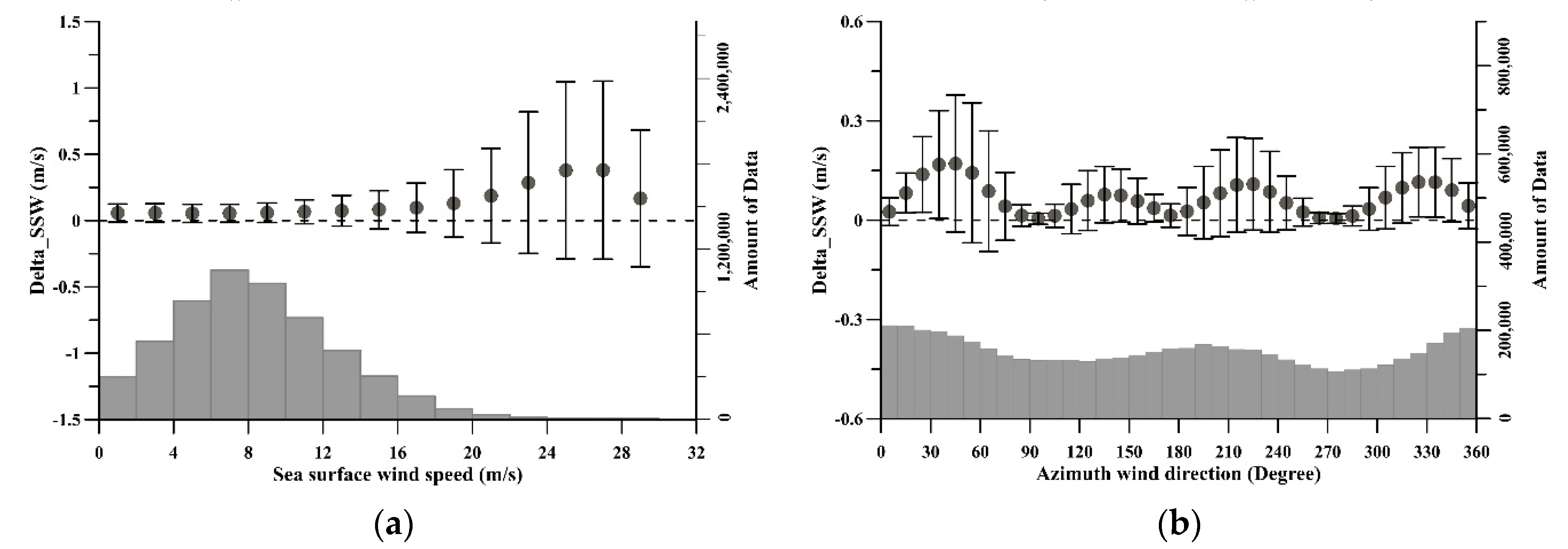
In the previous subsection, the S1 data and collocated ASACT wind direction data were employed to construct the BP network to retrieve SSWS. However, Figure 1 indicates that the collocation of S1 with ASCAT in the Arctic results in temporally and spatially irregular distributions. To apply the trained the BP network to all the acquired S1 data and for the operational retrievals in the Arctic MIZ, we will utilize reanalysis model sea surface wind direction data as an external input (i.e., to obtain and , as illustrated in Figure 3) to the neural network. Because the numerical model is uniform at both spatial and temporal scales, we can expect that each acquired S1 image can be collocated with the model results to obtain the external wind direction. However, the reanalysis wind data may have biases, which can induce uncertainty in the retrieval. The sea surface wind direction data from the reanalysis model are calculated based on the and components of the wind field. It is characterized that the ERA−5 has a zonal wind bias of approximately −0.10 m/s and meridional bias of approximately 0.25 m/s in the high latitude region of 70°N [30]. As the detailed values of the biases are not listed in 30, both numbers are approximately based on Figure 3 and Figure 4 in that work. We used the ERA−5 wind direction data (with a grid size of 0.25° and available by each hour) as the input to the trained BP network, and the retrieval was applied to the 11,431 S1 EW images. The results are denoted . By adding the zonal ( component) and meridional ( component) wind bias of the ERA5 data to the original dataset and applying the same retrieval procedure, we obtained the . The variations in with sea surface wind speed and azimuthal wind direction are shown in Figure 7a,b, respectively.
The parameter shows an overall increasing trend with wind speed. For an SSWS lower than approximately 19 m/s, the increasing trend is almost imperceptible, and the mean is smaller than 0.20 m/s with a maximum standard deviation of 0.25 m/s. When the SSWS is higher than approximately 20 m/s, the trend increases rapidly, and the largest mean reaches 0.38 m/s at a wind speed of 27 m/s. The reason for the decreased (in terms of both mean and standard deviation values) for a wind speed of 29 m/s is not clear. The number of collocated data in this bin is 4185, which is comparable to that in neighbor bins, e.g., there are 6359 and 6727 data pairs in the bins of 25 m/s and 27 m/s, respectively. The variation in along with the azimuthal wind direction (Figure 7b) shows a periodic fluctuation comprising a combination of sine and cosine functions of the azimuthal wind angle. Under various wind direction conditions, the is generally lower than 0.15 m/s.
4.4. Discrepancy in the SSWS Retrievals from S1A and S1B Data
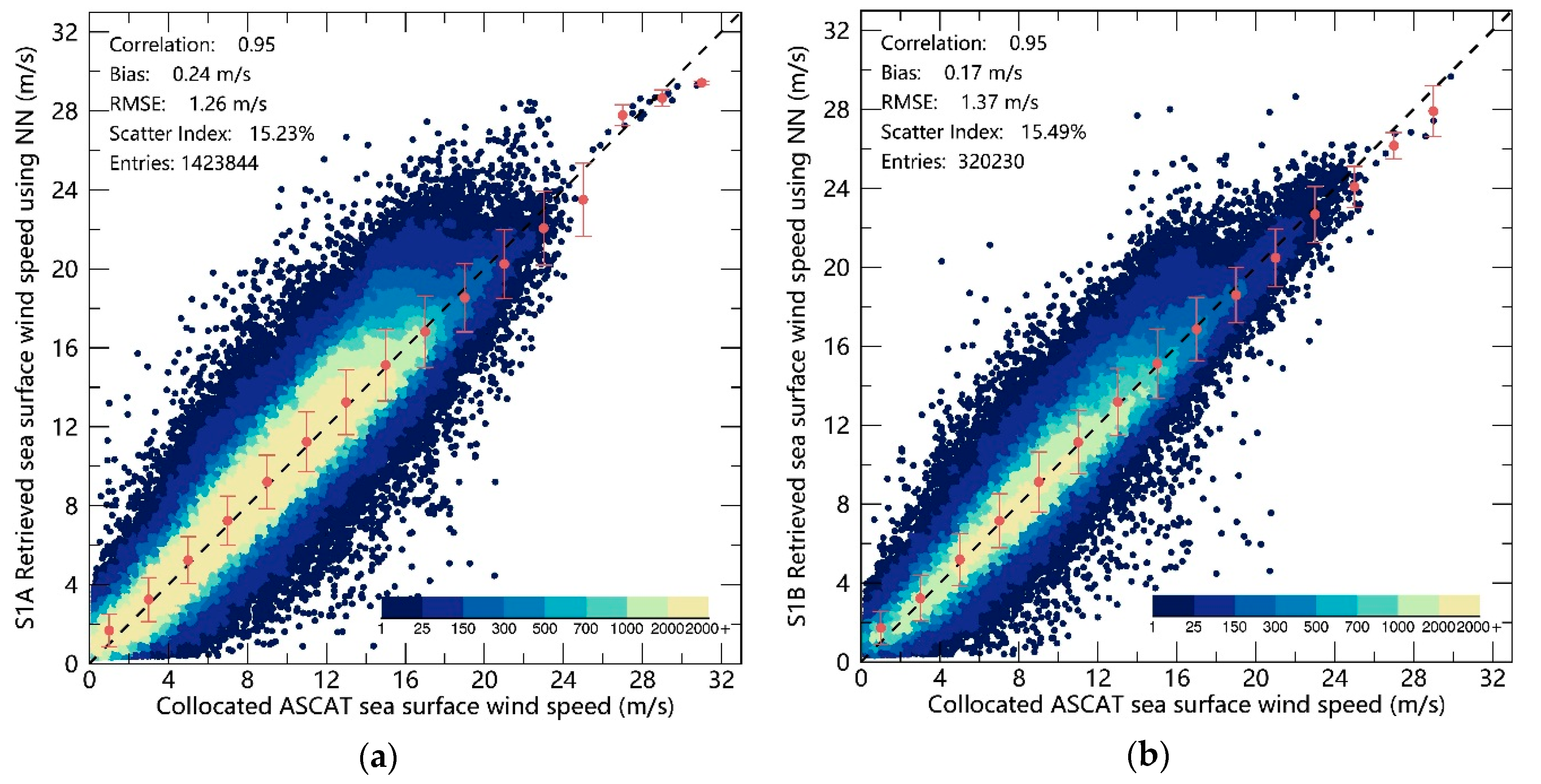
The twin satellites S1A and S1B are equipped with identical sensors, but their radiometric calibration accuracies have discrepancies. Both sensors’ radiometric calibrations have been verified independently. Based on point target measurements, a previous study in [21] showed that the overall absolute radiometric calibration accuracy of S1A co−polarization data for the stripmap (SM), IW, and EW modes is of 0.43 dB (1). Another study on the independent verification of S1B calibration [31] suggested that the absolute radiometric calibration accuracy of the S1B co−polarization data in EW mode (based on the second and third beams of the five swath beams) is 0.30 dB. These findings imply that the two sensors do have a discrepancy in their radiometric calibration, although the difference is only approximately 0.13 dB.
Figure 8 shows comparisons of the S1A and S1B retrieved with the collocated ASCAT wind speed. We did not discriminate between the training and testing data in these comparisons. The number of the S1A collocated data pairs with the ASCAT data is approximately four times that of S1B collocations. In fact, the discrepancy between the SSWS retrievals by the two sensors is almost negligible. The correlation and S.I. of the two comparisons are identical. The bias suggests that the S1B retrieved SSWS is closer to the ASCAT SSWS than that from the S1A (0.17 m/s versus 0.24 m/s), while the RMSE values of 1.37 m/s versus 1.26 m/s suggest that the S1A retrievals have slightly better agreement with the ASCAT data than the S1B retrievals.
5. Discussion
The BP neural network constitutes the basis of some machine learning models and is a good candidate for fitting nonlinear relations, making it suitable for deriving some geophysical parameters from satellite data. With respect to retrieving by spaceborne SAR data using a neural network, there are generally three sources of uncertainties.
First, there is uncertainty about which inputs are used. For instance, in a previous study [24], for inputs, the authors used SAR radar backscatter alone and both SAR backscatter and the collocated scatterometer wind direction. The retrieval results were significantly improved when the wind direction data were used as an input to the neural network (though the expression for inputting the wind direction remains unclear). Owing to long−term investigations on the retrieval of sea surface wind fields by scatterometer and SAR, various GMFs have been proposed, and the empirical relationship between radar backscatter and sea surface wind fields is clear. Therefore, we employed four parameters, namely, , , , and as inputs to the network. In our experiments, it was found that the training of the BP neural network rapidly reaches convergency, which can be partially attributed to using appropriate input parameters.
Second, determining the structure of the neural network is a challenge. Although it is well known that the BP neural network has three layers, designing the number of hidden layers and neurons is difficult. By necessity, we tested various combinations (e.g., the number of hidden layers was increased from two to three, and then to four) until the retrieval results (output) showed the best agreement with the collocated ASCAT wind speed which was based on two statistical parameters, the bias and RMSE. We eventually determined the current structure of the BP neural network for retrieving from S1 HH−polarized data. Nevertheless, designing the neural network to achieve the desired goals is challenging.
Finally, the distribution of SSWS is naturally unbalanced. Unfortunately, this problem cannot be fully resolved by simply expanding the training dataset. In fact, our more than 1.7 million collocated data pairs are sufficient to represent various sea surface wind conditions (e.g., as shown in Figure 4) and we also tried various combinations of data in different wind speed ranges to constitute the training dataset. Once there is a large enough number of training data, the neural network performance stabilizes, and the results generally remain unchanged even when more training data are added to the network (which may also induce overfitting). Compared with the proportion of low to moderate wind speed cases within the entire dataset, high wind speed cases (SSWS larger than 15 m/s) are rare. Hence, these rare cases are often neglected by the neural network as “noise”, as the training process is terminated based on the overall minimum MSE. As a result, the S1−retrieved SSWS is lower than the collocated ASCAT wind speeds for wind speeds higher than approximately 15 m/s. Moreover, the underestimation trend becomes more distinct with increasing wind speed, as presented in Figure 5a. It is known that sea surface wind field retrieval from SAR co−polarization data using a GMF may underestimate high wind speeds, e.g., in [32]. By duplicating the high wind cases in the training dataset, we arbitrarily enhanced their weights in the neural network. The retrieval results based on both the training and testing datasets suggest that this approach can partially solve the problem of underestimating sea surface wind retrievals by SAR co−polarization data.
Although the twin satellites S1A and S1B have some discrepancies in their radiometric calibration, our analysis by comparing their respective results of retrieved SSWS suggests the discrepancies between their retrievals are negligible. Since the release of S1 Instrument Processing Facility (IPF) version 2.90 (available from March 2018; referring to https://qc.sentinel1.eo.esa.int/ipf/), the noise vectors in both the range and azimuth directions have been provided in the EW mode data. Prior to the IPF version 2.90, only the noise vectors in the range direction were available in the EW data. This improvement in the noise estimation may lead to a more accurate calibration of the EW mode data. However, we did not treat the EW mode data acquired before and after March 2018 separately in the development of the neural network. We found that this improvement (providing noise vectors in the azimuth direction) in the noise estimation has a significant effect on the cross−polarization data in EW mode [33], e.g., by reducing the scalloping effect in the azimuth direction. Nevertheless, with the acquisitions of more S1 EW data, one may separate the two sensors’ data to develop their respective neural networks and compare the weights and biases of each neuron to ascertain the discrepancies in their SSWS retrievals.
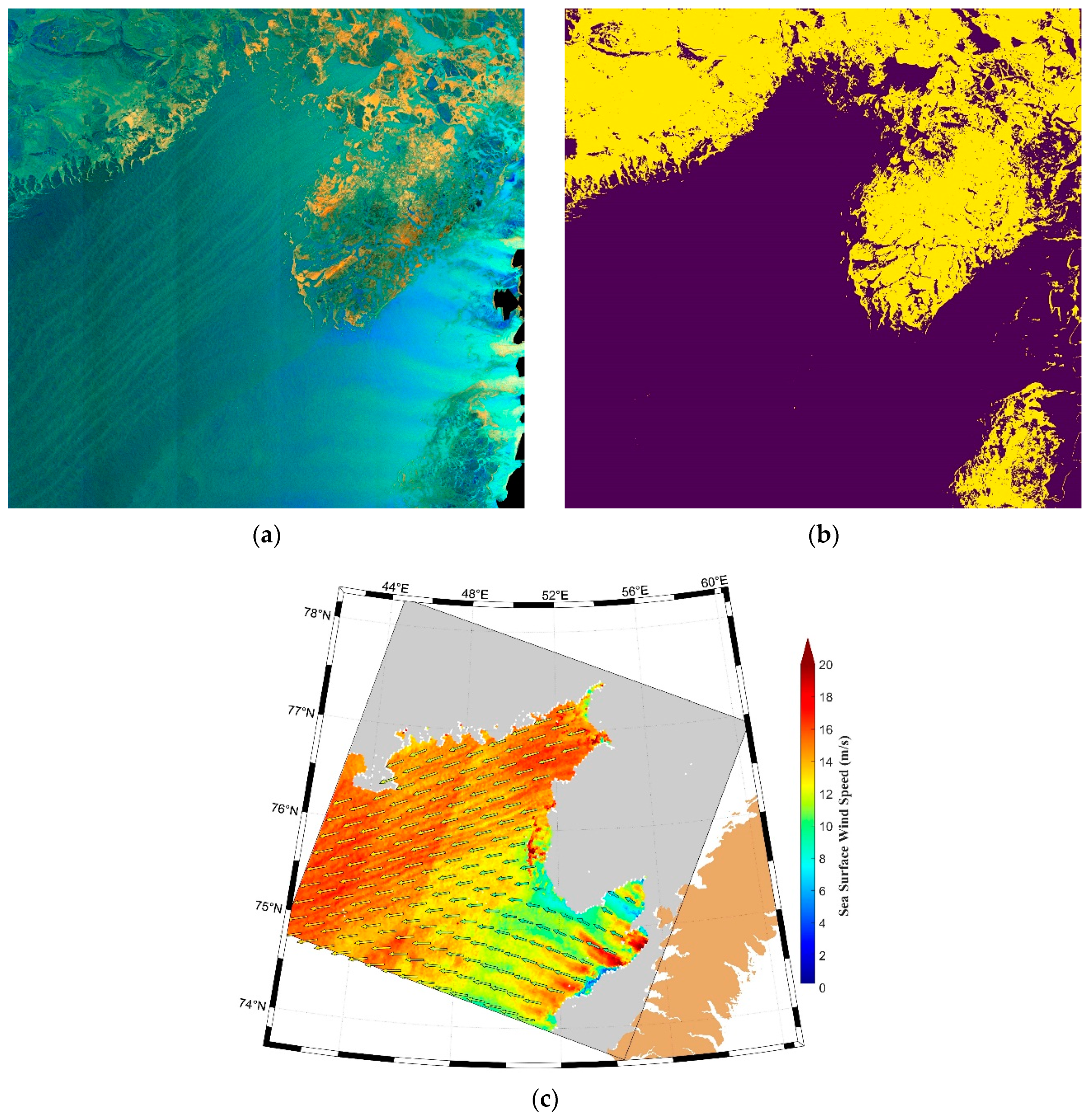
Thus far, we have used the IMS data to mask the sea ice cover. Notably, that the IMS data are daily available, which is based on multi−sensor observations within one day, while SAR observations represent snapshots. Therefore, the sea ice cover observed by spaceborne SAR deviates from the IMS data, because sea ice drifts. Figure 9 shows such a case. The S1 EW mode data were acquired in April 2018 over the Barents Sea. Figure 9a shows its false−color composite image based on three channels of HV (red), the difference between HH and HV (green) and the ratio of HH and HV (blue). Note that HV−polarized data of the EW mode over sea ice and open water areas are significantly disturbed by noise, and they should be denoised [33]. Based on the information in these three channels, we developed a deep−learning method (U−net) for discriminating sea ice cover and open water regions, as shown in Figure 9b, in which yellow represents sea ice cover with a spatial resolution of 200 m. While the algorithm is being tested and adjusted for a large dataset of the S1 dataset acquired in the Arctic to achieve accurate sea ice cover results, we currently used the IMS data to mask sea ice cover and conduct retrieval based on the developed BP neural network, as shown in Figure 9c, in which the gray tone represents the sea ice cover from the IMS data. Comparing (c) with (b), one can observe that the IMS sea ice cover is larger than the SAR observation, which is reasonable because sea ice drifts, and this discrepancy is particularly distinct in the MIZ. If open water areas are marked as sea ice cover, then we lose some sea surface wind information, as these areas are not used for retrievals. For areas that are sea ice cover as observed by SAR but they are not masked by the IMS (either due to the uncertainty of the IMS data or due to drift of sea ice over time), the subsequent processing step involving a homogeneity test after sea ice masking can further discard these areas and avoid biased retrievals.
6. Conclusion
With the rapid retreat of sea ice in the Arctic, the MIZ is drawing more attention, as the interaction between sea ice and ocean dynamics is significant and may have feedback affecting seasonal sea ice retreat in the Arctic. Therefore, sea surface wind data at high spatial resolution are highly desirable because of the lack of currently available ice and ocean remote sensing information from space for polar regions.
In this study, we presented a method for retrieving SSWS from S1 EW data in HH polarization based on a BP neural network. Unlike the data acquired over other sea areas where most EW mode data are a combination of VV and vertical−horizontal (VH) polarizations, the EW data acquired in the Arctic are a combination of HH and HV polarizations for intensive monitoring of sea ice.
Based on the rather well−developed GMFs for retrieving sea surface wind fields by spaceborne SAR data, we determined four parameters, i.e., the radar backscatter , the azimuthal sea surface wind direction in terms of and , and the incidence angle , to use as inputs to the neural network. The structure of the neural network was determined based on various trials. We duplicated the high wind cases in the training dataset to increase their influence on the network performance, which partially resolved the problems of underestimating for wind speeds above approximately 16 m/s. A comparison of the retrieved using the testing dataset (1,319,321 data pairs) with the collocated ASCAT wind speed yielded a bias of 0.23 m/s and an RMSE of 1.25 m/s. Although the overall bias suggests an overestimation over the ASCAT wind speeds, a stepwise comparison (indicated by the error bars in Figure 5d) suggests that the bias has a limited dependence on the wind speeds. Moreover, the saturation phenomenon of SSWS retrievals generally found in SAR co−polarization data using GMFs is not distinct in the retrievals (up to of approximately 30 m/s) using the BP neural network.
We further compared the S1−derived SSWS with the independent NDBC buoy measurements, in which a bias of 0.12 m/s and an RMSE of 1.42 m/s were obtained. Although the data pairs of S1 collocated with the measurements from the XueLong icebreaker acquired during the Arctic surveys are limited, their comparison revealed a similar RMSE value to that of the comparison with the NDBC buoy measurements.
Our next step is to produce a sea surface wind field product in the Arctic based on the S1 data acquired since its launch; accordingly, we have to use a reanalysis model wind direction data (which has uniform outputs in both space and time) as input to the developed BP neural network. Therefore, we preliminarily analyzed the effect of the bias of the ERA−5 reanalysis wind model on the retrieval of the S1 SSWS. Up to 19 m/s of SSWS, the induced absolute error of the retrieval is less than 0.25 m/s. With increasing wind speed, the increasing trend of the absolute error is obvious and can reach 0.38 m/s for an SSWS of 27 m/s. Interestingly, the induced absolute error exhibits a periodic variation in azimuthal wind direction, roughly follows a combination of sine and cosine functions.
While a denoising method for S1 EW data in HV polarization has recently been developed [33], both the HH and HV polarization information from the EW data acquired in the Arctic will be included in the BP neural network, which might facilitate better retrieval of high wind cases [32,34]. Along with developing a robust method for discriminating sea ice and open water from S1 EW data, we will combine this method with sea surface wind retrievals to obtain synergistic information on sea ice and ocean dynamic parameters in the MIZ of the Arctic.
Owing to the large volume of S1 data acquired over the globe, quantitative retrievals of dynamic parameters in the air–sea interface based on machine learning algorithms are drawing more attention. The present study demonstrates that the most common BP neural network can yield accurate retrievals of SSWS and can even somehow partially resolve the problem of underestimating high wind speeds which are often encountered when the conventional GMF methods are used. The information stored in the BP neural network is a set of numerical weights and connects among neurons in different layers. However, these weights and connections do not provide direct clues as to how the task (i.e., retrieval of SSWS using the S1 data) is performed or what the relationship is between inputs and outputs.
One issue that remains unresolved is that the proposed method still needs external wind direction data as inputs. We are in the era of big SAR data. Thus, deep learning might be one way to solve this issue, which has limited the retrievals of sea surface wind fields by spaceborne SAR for a few decades.
Author Contributions
Conceptualization, X.-M.L.; methodology, X.-M.L.; formal analysis, X.-M.L., T.Q., and K.W.; data curation, K.W.; writing—original draft preparation, X.-M.L.; writing—review and editing, X.-M.L.; supervision, X.-M.L.; project administration, X.-M.L.; funding acquisition, Y.L. All authors have read and agreed to the published version of the manuscript.
Funding
This work was supported in part by the National Key Research and Development Project (2018YFC1407100) China.
Acknowledgments
The S1 SAR data are downloaded from the Copernicus data hub (https://scihub.copernicus.eu/), and the ASCAT data are accessed from EUMETSAT. Use of the reference data of ERA−5 (https://cds.climate.copernicus.eu/cdsapp#!/home), IMS data (https://www.natice.noaa.gov/ims/) and GSHHG data (https://www.soest.hawaii.edu/pwessel/gshhg/) is also acknowledged.
Conflicts of Interest
The authors declare no conflict of interest.
Appendix A
In the following, the processing steps for retrieving SSWS from the S1 EW data using the developed BP neural network are provided. The MATLAB functions used are written in bold and italic.
Step 1: Reading the S1 data and conducting radiometric calibration
The digital number (DN) values () of the S1 data are read from the Geotiff data and the calibration vector (), noise vector (), latitude matrix (), longitude matrix (), incidence angle matrix (), and look angle () are read from the annotation files (.XML).
The S1 data are radiometrically calibrated using the following equation:
At the same time, the matrices of , , and are interpolated to grids, where each grid has a size of 2 km by 2 km.
Step 2: Masking and homogeneity test
We use coastline data from the Global Self−consistent, Hierarchical, High−resolution Geography Database (GSHHG) coastal line data [35] to mask the land area in the S1 images. Then, the IMS data are used to mask the sea ice cover. As mentioned in the main text, there are discrepancies in the sea ice cover between SAR observations and IMS data. On the other hand, there may exist other features that disturb the sea surface and make the data unsuitable for SSWS retrieval. So, we use the homogeneity factor [25] to exclude these grids from retrievals. The homogeneity factor is defined as:
And
We further divide each SAR sub−image (2 km × 2 km) into 2×2 sub−grids to calculate the homogeneity factor, i.e., in (A3). The image power spectrum of each sub−grid is estimated by a fast Fourier transform (FFT). The S1 sub−images with a homogeneity factor ≤1.05 are used for the retrieval. However, as this threshold is determined based on empirical experience (visual inspections), we have found that some retrievals are acceptable when their homogeneity factors are between 1.05 and 1.50. Therefore, the SSWS retrievals from the sub−images which have the homogeneity factor in this range ([1.05, 1.5]) are defined as “suspecting” results in the NetCDF product.
Step 3: Matching the S1 data with the ERA−5 reanalysis wind model data
Following the preprocessing in the above two steps, each S1 sub−image is temporally and spatially matched with the ERA−5 reanalysis wind data.
As the ERA−5 reanalysis wind model data is available each hour, the temporal difference between the S1 observation and the model is no larger than 30 min. With respect to spatial collocation, the and components of the ERA−5 wind data at the four (model) grids nearest to the S1 subimage are bilinearly interpolated to the location of the sub−image. Based on the and components, one can derive wind direction and the consequent azimuthal wind direction by taking into account the SAR looking angle.
After matching the S1 observations with the ERA−5 reanalysis wind data, each S1 sub−image has four inputs available, i.e., , , and for the trained BP neural network, which compose an array in MATLAB:
Step 4: Retrieval of SSWS using the BP neural network
We applied the MATLAB function mapminmax to scale the input to the range :
Then, we applied the MATLAB function sim to retrieve the SSWS:
The output of the neural network is a normalized retrieved SSWS and needs to be anti−normalized to obtain the true wind speed. We set the and max values of normalizing the sea surface wind speed to be 0 and 30. Note that setting of the maximum value of 30 m/s to normalize SSWS does not limit the retrievals cannot be over 30 m/s as the network can output values of larger than 1.0.
The weights and biases of the trained BP neural network are stored in the matrix , which are provided in the MATLAB code as supplementary to the preprint version of the manuscript: https://www.preprints.org/manuscript/202005.0300/v1.
References
- Stoffelen, A.; Anderson, D. Scatterometer data interpretation: Estimation and validation of the transfer function CMOD4. J. Geophys. Res. 1997, 102, 5767–5780. [Google Scholar] [CrossRef]
- Hersbach, H.; Stoffelen, A.; de Haan, S. An improved C-band scatterometer ocean geophysical model function: CMOD5. J. Geophys. Res. 2007, 112, C03006. [Google Scholar] [CrossRef]
- Hersbach, H. Comparison of C-Band Scatterometer CMOD5.N Equivalent Neutral Winds with ECMWF. J. Atmos. Ocean. Technol. 2010, 27, 721–736. [Google Scholar] [CrossRef]
- Elyouncha, A.; Neyt, X.; Stoffelen, A.; Verspeek, J. Assessment of the corrected CMOD6 GMF using scatterometer data. In Remote Sensing of the Ocean, Sea Ice, Coastal Waters, and Large Water Regions; International Society for Optics and Photonics: Toulouse, France, 2015; Volume 9638. [Google Scholar]
- Stoffelen, A.; Verspeek, J.A.; Vogelzang, J.; Verhoef, A. The CMOD7 geophysical model function for ASCAT and ERS wind retrievals. IEEE J. Sel. Top. Appl. Earth Observ. Remote Sens. 2017, 10, 2123–2134. [Google Scholar] [CrossRef]
- Quilfen, Y.; Chapron, B.; Elfouhaily, T.; Katsaros, K.; Tournadre, J. Observation of tropical cyclones by high-resolution scatterometry. J. Geophys. Res. 1998, 103, 7767–7786. [Google Scholar] [CrossRef]
- Elfouhaily, T.; Thompson, D.R.; Freund, D.E.; Vandemark, D.; Chapron, B. A new biastatic model for electromagnetic scattering from perfectly conducting random surfaces: Numerical evaluation and comparison with SPM. Waves Random Media 2001, 11, 33–43. [Google Scholar] [CrossRef] [Green Version]
- Mouche, A.A.; Hauser, D.; Daloze, J.F.; Guerin, C. Dual-polarization measurements at C-band over the ocean: Results from airborne radar observations and comparison with ENVISAT ASAR data. IEEE Trans. Geosci. Remote Sens. 2005, 43, 753–769. [Google Scholar] [CrossRef]
- Liu, G.H.; Yang, X.F.; Li, X.F.; Zhang, B.; Pichel, W.; Li, Z.W.; Zhou, X. A systematic comparison of the effect of polarization ratio models on sea surface wind retrieval from C-band synthetic aperture radar. IEEE J. Sel. Top. Appl. Earth Observ. Remote Sens. 2013, 6, 1100–1108. [Google Scholar] [CrossRef]
- Zhang, B.; Perrie, W.; He, Y.J. Wind speed retrieval from RADARSAT-2 quad-polarization images using a new polarization ratio model. J. Geophys. Res. 2011, 116, C08008. [Google Scholar] [CrossRef]
- Monaldo, F.M.; Thompson, D.R.; Pichel, W.G.; Clemente-Colon, P. A systematic comparison of QuikSCAT and SAR ocean surface wind speeds. IEEE Trans. Geosci. Remote Sens. 2004, 42, 283–291. [Google Scholar] [CrossRef]
- Zhang, B.; Mouchee, M.; Lu, Y.; Perriee, W.; Zhang, G.S.; Wang, H. A geophysical model function for wind speed retrieval from C-band HH-polarized synthetic aperture radar. IEEE Geosci. Remote Sens. Lett. 2019, 16, 1521–1525. [Google Scholar] [CrossRef]
- Isoguchi, M.; Shimada, M. An L-band ocean geophysical model function derived from PALSAR. IEEE Trans. Geosci. Remote Sens. 2009, 47, 1925–1936. [Google Scholar] [CrossRef]
- Li, X.-M.; Lehner, S. Algorithm for sea surface wind retrieval from TerraSAR-X and TanDEM-X data. IEEE Trans. Geosci. Remote Sens. 2014, 52, 2928–2939. [Google Scholar] [CrossRef] [Green Version]
- Strong, C.; Rigor, I.G. Arctic marginal ice zone trending wider in summer and narrower in winter. Geophys. Res. Lett. 2013, 40, 4864–4868. [Google Scholar] [CrossRef]
- Qin, T.T.; Li, X.-M.; Jia, T.; Feng, Q. Retrieval of ocean surface wind speed using Sentinel-1 HH polarization data. In Proceedings of the 2019 SAR in Big Data Era (BIGSARDATA), Beijing, China, 5–6 August 2019; pp. 1–4. [Google Scholar]
- Li, X.F.; Liu, B.; Zheng, G.; Ren, Y.B.; Zhang, S.S.; Liu, Y.G.; Gao, L.; Liu, Y.H.; Zhang, B.; Wang, F. Deep learning-based information mining from ocean remote sensing imagery. Nati. Sci. Rev. 2020. [Google Scholar] [CrossRef]
- ESA (European Space Agency), “Sentinel-1 product specification,” 2016. Available online: https://sentinel.esa.int/web/sentinel/document-library/content/-/article/sentinel-1-product-specification (accessed on 5 October 2020).
- Olivier, P.; Vidal-Madjar, D. Empirical estimation of the ERS-1 SAR radiometric resolution. Int. J. Remote Sens. 1994, 15, 1109–1114. [Google Scholar] [CrossRef]
- Moreira, A. Improved multi-look techniques applied to SAR and SCANSAR imagery. IEEE Trans. Geosci. Remote Sens. 1991, 29, 529–534. [Google Scholar] [CrossRef]
- Schwerdt, M.; Schmidt, K.; Ramon, N.T.; Alfonzo, G.C.; Doring, B.G.; Zink, M.; Prats-Iraola, P. Independent verification of the Sentinel-1A system calibration. IEEE J. Sel. Top. Appl. Earth Observ. Remote Sens. 2016, 9, 994–1007. [Google Scholar] [CrossRef] [Green Version]
- Helfrich, S.R.; McNamara, D.; Ramsay, B.H.; Baldwin, T.; Kasheta, T. Enhancements to and forthcoming developments in the Interactive Multisensor Snow and Ice Mapping System (IMS). Hydrol. Process. 2007, 21, 1576–1586. [Google Scholar] [CrossRef]
- Li, X.-M.; Sun, Y.; Zhang, Q. Extraction of sea ice cover by Sentinel-1 SAR based on SVM with unsupervised generation of training data. IEEE Trans. Geosci. Remote Sens. 2020. [Google Scholar] [CrossRef]
- Horstmann, J.; Schiller, H.; Schulz-Stellenfleth, J.; Lehner, S. Global wind speed retrieval from SAR. IEEE Trans. Geosci. Remote Sens. 2003, 41, 2277–2286. [Google Scholar] [CrossRef] [Green Version]
- Schulz-Stellenfleth, J.; Lehner, S. Measurement of 2-D sea surface elevation fields using complex synthetic aperture radar data. IEEE Trans. Geosci. Remote Sens. 2004, 42, 1149–1160. [Google Scholar] [CrossRef]
- Li, X.-M.; Lehner, S.; Bruns, T. Ocean wave integral parameter measurements using Envisat ASAR wave mode data. IEEE Trans. Geosci. Remote Sens. 2011, 49, 155–174. [Google Scholar] [CrossRef] [Green Version]
- Peixoto, J.P.; Oort, A.H. Physics of Climate; American Institute of Physics; AIP-Press: College Park, MD, USA, 1992; Volume 45. [Google Scholar] [CrossRef]
- Rumelhart, D.; Hinton, G.; Williams, R. Learning representations by back-propagating errors. Nature 1986, 323, 533–536. [Google Scholar] [CrossRef]
- Lu, Y.R.; Zhang, B.; Perrie, W.; Mouche, A.; Zhang, G.S. CMODH validation for C-band synthetic aperture radar HH polarization wind retrieval over the ocean. IEEE Geosci. Remote Sens. Lett. 2020, 99, 1–5. [Google Scholar] [CrossRef]
- Rivas, M.B.; Stoffelen, A.D. Characterizing ERA-Interim and ERA-5 surface wind biases using ASCAT. Ocean Sci. 2019, 15, 831–852. [Google Scholar] [CrossRef] [Green Version]
- Schwerdt, M.; Schmidt, K.; Ramon, N.T.; Klenk, P.; Yague-Martinez, N.; Prats-Iraola, P.; Zink, M.; Geudtner, D. Independent system calibration of Sentinel-1B. Remote Sens. 2017, 9, 511. [Google Scholar] [CrossRef] [Green Version]
- Vachon, P.W.; Wolfe, J. C-band Cross-Polarization Wind Speed Retrieval. IEEE Geosci. Remote Sens. Lett. 2011, 8, 456–459. [Google Scholar] [CrossRef]
- Sun, Y.; Li, X.-M. Denoising Sentinel-1 extra-wide mode cross-polarization images over sea ice. IEEE Trans. Geosci. Remote Sens. 2020. [Google Scholar] [CrossRef]
- Gao, Y.; Guan, C.; Sun, J.; Xie, L. A wind speed retrieval model for Sentinel-1A EW mode cross-polarization images. Remote Sens. 2019, 11, 153. [Google Scholar] [CrossRef] [Green Version]
- Wessel, P.; Smith, W.H.F. A global self-consistent, hierarchical, high-resolution shoreline database. J. Geophys. Res. 1996, 101, 8741–8743. [Google Scholar] [CrossRef] [Green Version]
Figure 1.
Spatial distributions of the S1A (a) and S1B (b) EW images collocated with the ASCAT measurements from 2015 to 2018.
Figure 1.
Spatial distributions of the S1A (a) and S1B (b) EW images collocated with the ASCAT measurements from 2015 to 2018.

Figure 2.
Radiometric resolution calculated using different cell sizes of the S1 EW data in HH polarization. The dashed line refers to the absolute calibration accuracy (0.43 dB) of S1 data.
Figure 2.
Radiometric resolution calculated using different cell sizes of the S1 EW data in HH polarization. The dashed line refers to the absolute calibration accuracy (0.43 dB) of S1 data.

Figure 3.
Structure of the BP neural network developed to retrieve SSWS from the S1 data.

Figure 4.
Histograms of the S1 SAR collocated ASCAT sea surface wind speed (a) and wind direction (b). The dark gray bars represent the distribution of the data (i.e., described in the main text) used to train the BP neural network.
Figure 4.
Histograms of the S1 SAR collocated ASCAT sea surface wind speed (a) and wind direction (b). The dark gray bars represent the distribution of the data (i.e., described in the main text) used to train the BP neural network.

Figure 5.
Comparison between the S1−retrieved SSWS with the collocated ASCAT data using different training datasets (a)–(c) and the testing dataset (d). Refer to the main text for detailed explanations.
Figure 5.
Comparison between the S1−retrieved SSWS with the collocated ASCAT data using different training datasets (a)–(c) and the testing dataset (d). Refer to the main text for detailed explanations.


Figure 6.
Comparisons of the S1−retrieved SSWS using the developed BP neural network with the NDBC buoy measurements (a) and with the in situ measurements acquired by the XueLong icebreaker during its Arctic surveys (b).
Figure 6.
Comparisons of the S1−retrieved SSWS using the developed BP neural network with the NDBC buoy measurements (a) and with the in situ measurements acquired by the XueLong icebreaker during its Arctic surveys (b).

Figure 7.
Variations in along with ERA−5 reanalysis sea surface wind speed (a) and azimuthal wind direction (b).
Figure 7.
Variations in along with ERA−5 reanalysis sea surface wind speed (a) and azimuthal wind direction (b).

Figure 8.
Comparisons between the retrieved SSWS and the collocated ASCAT wind speed based on the S1A (a) and S1B (b) data.
Figure 8.
Comparisons between the retrieved SSWS and the collocated ASCAT wind speed based on the S1A (a) and S1B (b) data.

Figure 9.
A case of S1 EW data acquired over the Barents Sea to demonstrate the combination of sea ice cover detection and SSWS retrieval. (a) is a false−color composite image based on the HV and HH−polarized images (refer to the main text for details). (b) shows the discrimination of sea ice cover (yellow) and open water (purple) based on the EW data, and (c) is the sea surface wind map of the case, where the gray tone represents the sea ice cover from the IMS data (note its discrepancy with the result in (b)). The color of the background is the retrieved SSWS using the developed BP neural network. The ERA−5 reanalysis wind field (colored arrows) in synoptic time is superimposed on the plot for comparison. The ERA−5 wind direction data are used as input to the BP neural network. The image ID of this case is S1A_EW_GRDM_1SDH_20180404T034739_20180404T034839_021312_024AC5_A80C.


Table 1.
Results of our previous analysis of the retrievals of SSWS by using S1 data in HH polarization compared with NDBC buoy data and Advanced Scatterometer (ASCAT) data using different methods.
Table 1.
Results of our previous analysis of the retrievals of SSWS by using S1 data in HH polarization compared with NDBC buoy data and Advanced Scatterometer (ASCAT) data using different methods.
| Methods | Bias (m/s) | RMSE (m/s) | Scatter Index (S.I.) (%) | |
|---|---|---|---|---|
| Compared with Buoy (130 S1 images from October 2014 to December 2018) | PR in [8] + CMOD5.N | 0.13 | 1.63 | 23.42 |
| PR in [10] + CMOD5.N | −0.33 | 1.50 | 21.09 | |
| CMODH | −0.31 | 1.48 | 20.89 | |
| Compared with ASCAT (2277 S1 images from June to December 2018 in the Arctic MIZ) | PR in [8] + CMOD5.N | 0.41 | 1.70 | 18.85 |
| PR in [10] + CMOD5.N | −0.09 | 1.40 | 16.26 | |
| CMODH | −0.35 | 1.39 | 15.82 |
Table 2.
List of the NSBC buoys used to validate the S1 retrieved SSWS.
| Station | Latitude (°) | Longitude (°) | Height (m) | Station | Latitude (°) | Longitude (°) | Height (m) |
|---|---|---|---|---|---|---|---|
| 46022 | 40.720 N | −124.531 W | 4 | 46047 | 32.398 N | −119.498 W | 5 |
| 46014 | 39.233 N | −123.967 W | 4 | 46029 | 46.143 N | −124.485 W | 5 |
| 46013 | 38.238 N | −123.307 W | 4 | 46041 | 47.353 N | −124.742 W | 5 |
| 46015 | 42.779 N | −124.874 W | 4 | 51003 | 19.289 N | −160.569 W | 5 |
| 46050 | 44.677 N | −124.515 W | 4 | 51000 | 23.535 N | −153.781 W | 5 |
| 46092 | 36.751 N | −122.029 W | 4 | 44258 | 44.500 N | −63.400 W | 5 |
| 46025 | 33.749 N | −119.053 W | 4 | 45138 | 49.540 N | −65.710 W | 5 |
| 51004 | 17.602 N | −152.395 W | 4 | SMKF1 | 24.628 N | −81.109 W | 6.1 |
| 32303 | 5.000 N | −95.000 W | 4 | VCAF1 | 24.711 N | −81.107 W | 6.5 |
| 43301 | 8.000 N | −95.000 W | 4 | NPSF1 | 26.132 N | −81.807 W | 6.5 |
| 51002 | 17.037 N | −157.696 W | 4 | MTBF1 | 27.661 N | −82.594 W | 6.7 |
| 46035 | 57.026 N | −177.738 W | 5 | LONF1 | 24.844 N | −80.864 W | 7 |
| 46027 | 41.852 N | −124.382 W | 5 | VCVA2 | 57.125 N | −170.285 W | 8.5 |
| 46089 | 45.925 N | −125.771 W | 5 | CDRF1 | 29.136 N | −83.029 W | 10 |
| 46011 | 34.956 N | −121.019 W | 5 | VENF1 | 27.072 N | −82.453 W | 11.6 |
| 46028 | 35.712 N | −121.858 W | 5 | SANF1 | 24.456 N | −81.877 W | 14.6 |
| 46042 | 36.785 N | −122.398 W | 5 | MLRF1 | 25.012 N | −80.376 W | 15.8 |
| 46069 | 33.674 N | −120.212 W | 5 | PLSF1 | 24.693 N | −82.773 W | 17.7 |
| 46086 | 32.491 N | −118.035 W | 5 |
© 2020 by the authors. Licensee MDPI, Basel, Switzerland. This article is an open access article distributed under the terms and conditions of the Creative Commons Attribution (CC BY) license (http://creativecommons.org/licenses/by/4.0/).
Share and Cite
MDPI and ACS Style
Li, X.-M.; Qin, T.; Wu, K. Retrieval of Sea Surface Wind Speed from Spaceborne SAR over the Arctic Marginal Ice Zone with a Neural Network. Remote Sens. 2020, 12, 3291. https://0-doi-org.brum.beds.ac.uk/10.3390/rs12203291
AMA Style
Li X-M, Qin T, Wu K. Retrieval of Sea Surface Wind Speed from Spaceborne SAR over the Arctic Marginal Ice Zone with a Neural Network. Remote Sensing. 2020; 12(20):3291. https://0-doi-org.brum.beds.ac.uk/10.3390/rs12203291
Chicago/Turabian StyleLi, Xiao-Ming, Tingting Qin, and Ke Wu. 2020. "Retrieval of Sea Surface Wind Speed from Spaceborne SAR over the Arctic Marginal Ice Zone with a Neural Network" Remote Sensing 12, no. 20: 3291. https://0-doi-org.brum.beds.ac.uk/10.3390/rs12203291
Note that from the first issue of 2016, this journal uses article numbers instead of page numbers. See further details here.