VddNet: Vine Disease Detection Network Based on Multispectral Images and Depth Map


1
INSA-CVL, University of Orléans, PRISME, EA 4229, F18022 Bourges, France
2
INSA-CVL, University of Orléans, PRISME, EA 4229, F45072 Orléans, France
*
Author to whom correspondence should be addressed.
Remote Sens. 2020, 12(20), 3305; https://0-doi-org.brum.beds.ac.uk/10.3390/rs12203305
Submission received: 15 September 2020
/
Revised: 5 October 2020
/
Accepted: 6 October 2020
/
Published: 11 October 2020
(This article belongs to the Special Issue Advanced Deep Learning Strategies for the Analysis of Remote Sensing Images)
Abstract
:Vine pathologies generate several economic and environmental problems, causing serious difficulties for the viticultural activity. The early detection of vine disease can significantly improve the control of vine diseases and avoid spread of virus or fungi. Currently, remote sensing and artificial intelligence technologies are emerging in the field of precision agriculture. They offer interesting potential for crop disease management. However, despite the advances in these technologies, particularly deep learning technologies, many problems still present considerable challenges, such as semantic segmentation of images for disease mapping. In this paper, we present a new deep learning architecture called Vine Disease Detection Network (VddNet). It is based on three parallel auto-encoders integrating different information (i.e., visible, infrared and depth). Then, the decoder reconstructs and retrieves the features, and assigns a class to each output pixel. An orthophotos registration method is also proposed to align the three types of images and enable the processing by VddNet. The proposed architecture is assessed by comparing it with the most known architectures: SegNet, U-Net, DeepLabv3+ and PSPNet. The deep learning architectures were trained on multispectral data from an unmanned aerial vehicle (UAV) and depth map information extracted from 3D processing. The results of the proposed architecture show that the VddNet architecture achieves higher scores than the baseline methods. Moreover, this study demonstrates that the proposed method has many advantages compared to methods that directly use the UAV images.
1. Introduction
In agricultural fields, the main causes of losing quality and yield of harvest are virus, bacteria, fungi and pest [1]. To prevent these harmful pathogens, farmers generally treat the global crop to prevent different diseases. However, using a large amount of chemicals has a negative impact on human health and ecosystems. This constitutes a significant problem to be solved; precision agriculture presents an interesting alternative.
In recent decades, the precision agriculture [2,3] has introduced many new farming methods to improve and optimize crop yields, constituting a research field in continuous evolution. New sensing technologies and algorithms have enabled the development of several applications such as water stress detection [4], vigour evaluation [5], estimation of evaporate-transpiration and harvest coefficient [6], weed localization [7,8], and disease detection [9,10].
Disease detection in vine is an important topic in precision agriculture [11,12,13,14,15,16,17,18,19,20,21,22]. The aim is to detect and treat the infected area at the right place and the right time, and with the right dose of phytosanitary products. At the early stage, it is easier to control diseases with small amounts of chemical products. Indeed, intervention before infection spreads offers many advantages, such as preservation of vine, grap production and environment, and reducing the economics losses. To achieve this goal, frequent monitoring of the parcel is necessary. Remote sensing (RS) methods are among the most widely used for that purpose and essential in the precision agriculture. RS images can be obtained at leaf- or parcel-scale. At the leaf level, images are acquired using a photo sensor, either held by a person [23] or mounted on a mobile robot [24]. At the parcel level, satellite was the standard RS imaging system [25,26]. Recently, drones or UAVs have gained popularity due to their low cost, high-resolution images, flexibility, customization and easy data access [27]. In addition, unlike satellite imaging, UAV does not have the cloud problem, which has helped to solve many remote sensing problems.
Parcels monitoring generally requires orthophotos building from geo-referenced visible and infrared UAV images. However, two separated sensors generate a spatial shift between images of the two sensors. This problem also occurred after building the orthophotos. It has been established that it is more interesting to combine the information from the two sensors to increase the efficiency of disease detection. Therefore, image registration is required.
The existent algorithms of registration rely on an approach based on either the area or feature methods. The most commonly used in the precision agriculture are feature-based methods, which are based on matching features between images [28]. In this study, we adopted the feature-based approach to align orthophotos of the visible and infrared ranges. Then, the two are combined for the disease detection procedure, where the problem consists of assigning a class-label to each pixel. For that purpose, the deep learning approach is currently the most preferred approach for solving this type of problem.
Deep learning methods [29] have achieved a high level of performance in many applications, in which different network architectures have been proposed. For instance, R-CNN [30], Siamese [31], ResNet [32], SegNet [33] are architectures used for object detection, tracking, classification and segmentation, respectively, which operate in most cases in visible ranges. However, in certain situations, the input data are not only visible images but can be combined with multispectral or hyperspectral images [34], and even depth information [35]. In these contexts, the architectures can undergo modification for improving the methods [36]. Thus, in some studies [37,38,39,40], depth information is used as input data. These data generally provide precious information about scene or environment.
Depth or height information is extracted from the 3D reconstruction or photogrammetry processing. In UAV remote sensing imagery, the photogrammetry processing can to build a digital surface model (DSM) before creating the orthophoto. The DSM model can provide much information about the parcel, such as the land variation and objects on its surface. Certain research works have shown the ability to extract vinerows by generating a depth map from the DSM model [41,42,43]. These solutions have been proposed to solve the vinerows misextraction resulting from the NDVI vegetation index. Indeed, in some situations, the NDVI method cannot be used to extract vinerows when the parcel has a green grassy soil. The advantage of the depth map is its ability to separate areas above-ground from the ground, even if the color is the same for all zones. To date, there has been no work on the vine disease detection that combines depth and multispectral information with a deep learning approach.
This paper presents a new system for vine disease detection using multispectral UAV images. It combines a highly accurate orthophotos registration method, a depth map extraction method and a deep learning network adapted to the vine disease detection data.
The article is organized as follows. Section 2 presents a review of related works. Section 3 describes the materials and methods used in this study. Section 4 details the experiments. Section 5 discusses the performances and limitations of the proposed method. Finally, Section 6 concludes the paper and introduces ideas to improve the method.
2. Related Work
Plant disease detection is an important issue in precision agriculture. Much research has been carried out and a large survey has been realised by Mahlein (2016) [44], Kaur et al. (2018) [45], Saleem et al. (2019) [46], Sandhu et al. (2019) [47] and Loey et al. (2020) [48]. Schor et al. (2016) [49] presented a robotic system for detecting powdery mildew and wilt virus in tomato crops. The system is based on an RGB sensor mounted on a robotic arm. Image processing and analysis were developed using the principal component analysis and the coefficient of variation algorithms. Sharif et al. (2018) [50] developed a hybrid method for disease detection and identification in citrus plants. It consists of lesion detection on the citrus fruits and leaves, followed by a classification of the citrus diseases. Ferentinos (2018) [51] and Argüeso et al. (2020) [52] built a CNN model to perform plant diagnosis and disease detection using images of plant leaves. Jothiaruna et al. (2019) [53] proposed a segmentation method for disease detection at the leaf scale using a color features and region-growing method. Pantazi et al. (2019) [54] presented an automated approach for crop disease identification on images of various leaves. The approach consists of using a local binary patterns algorithm for extracting features and performing classification into disease classes. Abdulridha et al. (2019) [55] proposed a remote sensing technique for the early detection of avocado diseases. Hu et al. (2020) [56] combined an internet of things (IoT) system with deep learning to create a solution for automatically detecting various crop diseases and communicating the diagnostic results to farmers.
Disease detection in vineyards has been increasingly studied in recent years [11,12,13,14,15,16,17,18,19,20,21,22]. Some works are realised at the leaf scale, and others at the crop scale. MacDonald et al. (2016) [11] used a Geographic Information System (GIS) software and multispectral images for detecting the leafroll-associated virus in vine. Junges et al. (2018) [12] investigated vine leaves affected by the esca in hyperspectral ranges and di Gennaro et al. (2016) [13] worked at the crop level (UAV images). Both studies concluded that the reflectance of healthy and diseased leaves is different. Albetis et al. (2017) [14] studied the Flavescence dorée detection in UAV images. The results obtained showed that the vine disease detection using aerial images is feasible. The second study of Albetis et al. (2019) [15] examined of the UAV multispectral imagery potential in the detection of symptomatic and asymptomatic vines. Al-Saddik has conducted three studies on vine disease detection using hyperspectral images at the leaf scale. The aim of the first one (Al-Saddik et al. 2017) [16] was to develop spectral disease indices able to detect and identify the Flavescence dorée on grape leaves. The second one (Al-Saddik et al. 2018) [17] was performed to differentiate yellowing leaves from leaves diseased by esca through classification. The third one (Al-saddik et al., 2019) [18] consisted of determining the best wavelengths for the detection of the Flavescence dorée disease. Rançon et al. (2019) [19] conducted a similar study for detecting esca disease. Image sensors were embedded on a mobile robot. The robot moved along the vinerows to acquire images. To detect esca disease, two methods were used: the scale Invariant Feature Transform (SIFT) algorithm and the MobileNet architecture. The authors concluded that the MobileNet architecture provided a better score than the SIFT algorithm. In the framework of previous works, we have realized three studies on vine disease detection using UAV images. The first one (Kerkech et al. 2018) [20] was devoted to esca disease detection in the visible range using the LeNet5 architecture combined with some color spaces and vegetation indices. In the second study (Kerkech et al. 2019) [21], we used near-infrared images and visible images. Disease detection was considered as a semantic segmentation problem performed by the SegNet architecture. Two parallel SegNets were applied for each imaging modality and the results obtained were merged to generate a disease map. In (Kerkech et al. 2020) [22], a correction process using a depth map was added to the output of the previous method. Post-processing with these depth information demonstrated the advantage of this approach in reducing detection errors.
3. Materials and Methods
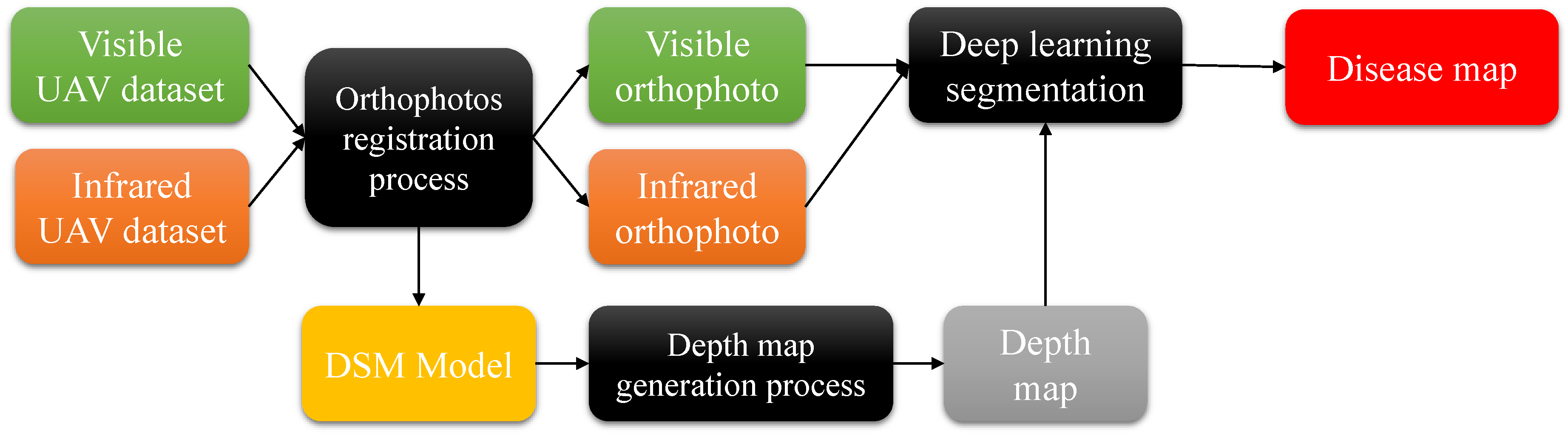
This section presents the materials and each component of the vine disease detection system. Figure 1 provides an overview of the methods. It includes the following steps: data acquisition, orthophotos registration, depth map building and orthophotos segmentation (disease map generation). The next sections detail these different steps.
3.1. Data Acquisition
Multispectral images are acquired using a quadricopter UAV that embeds a MAPIR Survey2 camera and a Global Navigation Satellite System (GNSS) module. This camera integrates two sensors in the visible and infrared ranges with a resolution of 16 megapixels (4608 × 3456 pixels). The visible sensor captures the red, green, and blue (RGB) channels and the infrared sensor captures the red, green, and near-infrared (R-G-NIR) channels. The wavelength of the near-infrared channel is 850 nm. The accuracy of the GNSS module is approximately 1 m.
The acquisition protocol consists of a drone flying over vines at an altitude of 25 m and at an average speed of 10 km/h. During flights, the sensors acquire an image every 2 s. Each image has a 70% overlap with the previous and the next ones. Each point of the vineyard has six different viewpoints (can be observed on six different images). The flight system is managed by a GNSS module. The flight plans include topographic monitoring aimed at guaranteeing a constant distance from the sol. Images are recorded with their GNSS position. Flights are performed at the zenith to avoid shadows, and with moderate weather conditions (light wind and no rain) to avoid UAV flight problems.
3.2. Orthophotos Registration
The multispectral acquisition protocol using two sensors causes a shift between visible and infrared images. Hence, a shift in multispectral images automatically implies a shift in orthophotos. Usually, the orthophotos registration is performed manually using the QGIS software. The manual method is time-consuming, requires a high focus to select many key points between visible and infrared orthophotos, and the result is not very accurate. To overcome this problem, a new method for automatic and accurate orthophotos registration is proposed.
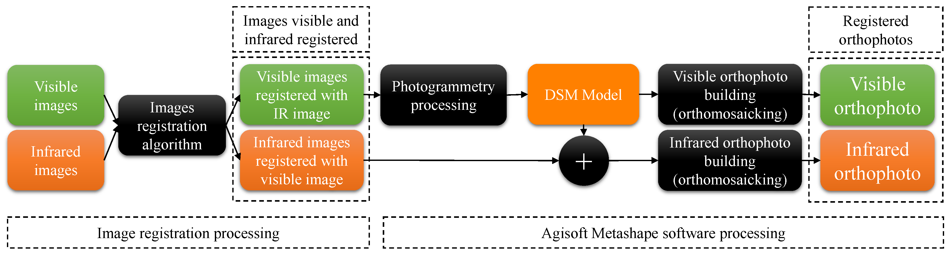
The proposed orthophotos registration method is illustrated in Figure 2 and is divided into two steps. The first one concerns the UAV multispectral images registration and the second permits the building of registered multispectral orthophotos. In this study, the first step uses the optimized multispectral images registration method proposed in [21]. Based on the Accelerated-KAZE (AKAZE) algorithm, the registration method uses feature-matching between visible and infrared images to match key points extracted from the two images and compute the homographic matrix for geometric correction. In order to increase accuracy, the method uses an iterative process to reduce the Root Mean Squared Error (RMSE) of the registration. The second step consists of using the Agisoft Metashape software to build and obtain the registered visible and infrared orthophotos. The Metashape software is based on the Structure from motion (SfM) algorithm for the photogrammetry processing. Building orthophotos requires the UAV images and the digital surface model (DSM). To obtain this DSM model, the software must go through a photogrammetry processing and perform the following steps: alignment of the images to build a sparse point cloud, then a dense point cloud, and finally the DSM. The orthophotos building is carried out by the option “build orthomosaic” process in the software. To build the visible orthophotos, it is necessary to use the visible UAV images and the DSM model, while, to build a registered infrared orthophoto, it is necessary to use the registered infrared UAV images and the same DSM model of the visible orthophoto. The parameters used in the Metashape software are detailed in Table 1.
3.3. Depth Map
The DSM model previously built in the orthophotos registration process is used here to obtain the depth map. In fact, the DSM model represents the terrain surface variation and includes all objects found here (in this case, objects are vine trees). Therefore, some processings are required to determine only the vine height. To extract the depth map from the DSM, the method proposed in [41] is used. It consists of applying the following processings: the DSM is first filtered using a low-pass filter of size 20 × 20; this filter is chosen to smooth the image and keep only the terrain surface variations, also called the digital terrain model (DTM). The DTM is thereafter subtracted from the DSM to eliminate the terrain variations and retain only the vine height. Due to the weak contrast of the result, an enhancement processing was necessary. The contrast is enhanced here by using a histogram-based (histogram normalization) method. The obtained result is an image with a good difference in grey levels between vines and non-vines. Once the contrast is corrected, an automatic thresholding using the Otsu’s algorithm is applied to obtain a binary image representing the depth map.
3.4. Segmentation and Classification
The last stage of the vine disease detection system concerns the data classification. This step is performed using a deep learning architecture for segmentation. Deep learning has proven its performance in numerous research studies and in various domains. Many architectures have been developed, such as SegNet [33], U-Net [57], DeepLabv3+ [58], and PSPNet [59]. Each architecture can provide good results in a specific domain and be less efficient in others. These architectures are generally used for the segmentation of complex indoor/outdoor scenes, medical ultrasound images, or even in agriculture. One channel is generally used for greyscale medical imaging or three channels for visible RGB color images. Hence, they are not always adapted to a specific problem. Indeed, for this study, multispectral and depth map data offer additional information. This can improve the segmentation representation and the final disease map result. For this purpose, we have designed our deep learning architecture adapted to the vine disease detection problem, and we have compared it to the most well known deep learning architectures. In the following sections, we describe the proposed deep learning architecture and the training process.
3.4.1. VddNet Architecture
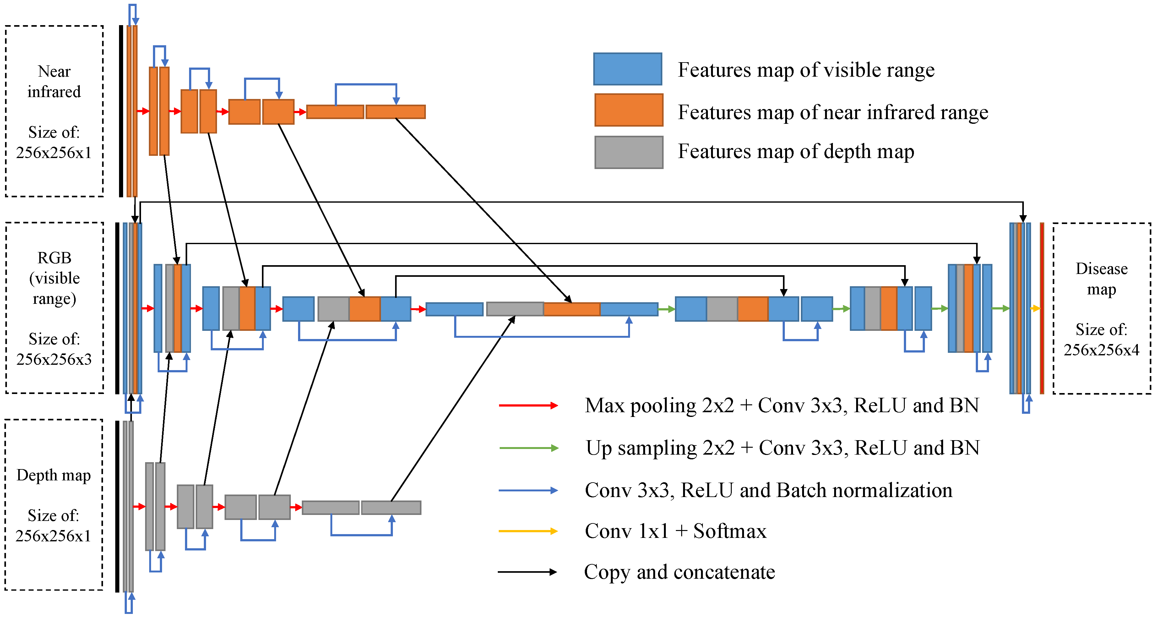
Vine Disease Detection Network (VddNet), Figure 3 is inspired by VGG-Net [60], SegNet [33], U-Net [57] and the parallel architectures proposed in [37,61,62,63]. VddNet is a parallel architecture based on the VGG encoder; it has three types of data as inputs: visible a RGB image, a near-infrared image and a depth map. VddNet is dedicated to segmentation, so the output has the same input, with a number of channels equal to the number of classes (4). It is designed with three parallel encoders and one decoder. Each encoder can typically be considered as a convolutional neural network without the fully connected layers. The convolutional operation is repeated twice using a 3 × 3 mask, a rectified linear unit (ReLU), a batch normalization and a subsampling using a max pooling function of 2 × 2 size and a stride of 2. The number of feature map channels is doubled at each subsampling step. The idea of VddNet is to encode each type of data separately and, at the same time, concatenate the near-infrared and the features map of the depth map with the visible features map before each subsampling. Hence, the central encoder preserves the features of the near-infrared and the depth map data merged with the visible features map, and concatenated at the same time. The decoder phase consists of upsampling and convolution with a 2 × 2 mask. It is then followed by two convolution layers with a 3 × 3 mask, a rectified linear unit, and a batch normalization. In contrast to the encoder phase, after each upsampling operation, the number of features map channels is halved. Using the features map concatenation technique of near-infrared and depth map, the decoder retrieves features lost during the merging and the subsample process. The decoder follows the same steps until it reaches the final layer, which is a convolution with a 1 × 1 mask and a softmax providing classes probabilities, at pixel-wise.
3.4.2. Training Dataset
In this study, one crop is used for model training and validation, and two crops for testing. To build the training dataset, four steps are required: data source selection, classes definition, data labelling, and data augmentation.
The first step is probably the most important one. Indeed, to allow a good learning, the data source for feeding models must represent the global data in terms of richness, diversity and classes. In this study, a particular area was chosen that contains a slight shadow area, brown ground (soil) and a vine partially affected by mildew.
Once the data source has been selected, it is necessary to define the different classes present in these data. For that purpose, each type of data (visible, near-infrared and depth map) is important in this step. In visible and near-infrared images, four classes can be distinguished. On the other hand, the depth map contains only two distinct classes, which are the vine canopy and the non-vine. Therefore, the choice of classes must match all data types. Shadow is the first class; it is any dark zone. It can be either on the vine or on the ground. This class was created to avoid confusion and misclassification on a non-visible pattern. Ground is the second class; from one parcel to another, ground is generally different. Indeed, the ground can have many colors: brown, green, grey, etc. To solve this color confusion, the ground is chosen as any pixels in the non-vine zone from the depth map data. Healthy vine is the third class; it is the green leaves of the vine. Usually, it is easy to classify these data, but when ground is also green, this leads to confusion between vine and ground in 2D images. To avoid that, the healthy class is defined as the green color in the visible spectrum and belonging to the vine canopy according to the depth map. The fourth and last class corresponds to diseased vine. Disease symptoms can present several colors in the visible range: yellow, brown, red, golden, etc. In the near-infrared, it is only possible to differentiate between healthy and diseased reflectances. In general, diseased leaves have a different reflectance than healthy leaves [17], but some confusion between disease and ground classes may occur when the two colors are similar. Ground must also be eliminated from the disease class using the depth map.
Data labelling was performed with the semi-automatic labelling method proposed in [21]. The method consists of using automatic labelling in a first step, followed by manual labelling in a second step. The first step is based on the deep learning LeNet-5 [64] architecture, where the classification is carried out using a 32 × 32 sliding window and a 2 × 2 stride. The result is equivalent to a coarse image segmentation which contains some misclassifications. To refine the segmentation, output results were manually corrected using the Paint.Net software. This task was conducted based on the ground truth (realized in the crop by a professional reporting occurred diseases), and observations in the orthophotos.
The last stage is the generation of a training dataset from the labelled data. In order to enrich the training dataset and avoid an overfitting of networks, data augmentation methods [65] are used in this study. A 256 × 256 pixels patches dataset is generated from the data source matrix and its corresponding labelled matrix. The data source consists of multimodal and depth map data and has a size of 4626 × 3904 × 5. Four data augmentation methods are used: translation, rotation, under and oversampling, and brightness variation. Translation was performed with an overlap of 50% using a sliding window in the horizontal and vertical displacements. The rotation angle was set at 30°, 60° and 90° Under- and oversampling were parametrized to obtain 80% and 120% of the original data size. Brightness variation is only applied to multispectral data. Pixel values are multiplied by the coefficients of 0.95 and 1.05, which introduce a brightness variation of ±5%. Each method brings an effect on the data (translation, rotation, etc.), allowing the networks to learn, respectively, transition, vinerows orientations, acquisition scale variation and weather conditions. At the end, the data augmentation generated 35.820 patches.
4. Experimentations and Results
This section presents the different experimental devices, as well as qualitative and quantitative results. The experiments are performed on Python 2.7 software, using the Keras 2.2.0 library for the development of deep learning architectures, and GDAL 3.0.3 for the orthophotos management. The Agisoft Metashape software version 1.6.2 is also used for photogrammetry processing. The codes were developed under the Linux Ubuntu 16.04 LTS 64-bits operating system and run on a hardware with an Intel Xeon 3.60 GHz × 8 processor, 32 GB RAM, and a NVidia GTX 1080 Ti graphics card with 11 GB of internal RAM. The cuDNN 7.0 library and the CUDA 9.0 Toolkit are used for deep learning processing on GPU.
4.1. Orthophotos Registration and Depth Map Building
To realize this study, multispectral and depth map orthophotos were required. Two parcels were selected and data were aquired at two different times to construct the orthophotos dataset. Each parcel had one or more of the following characteristics: with or without shadow, green or brown ground, healthy or partially diseased. Registered visible and infrared orthophotos were built from multispectral images using the optimized image registration algorithm [21] and the Agisoft Metashape software version 1.6.2. Orthophotos were saved in the geo-referenced file format “TIFF”. The parameters used in the Metashape software are listed in Table 1.
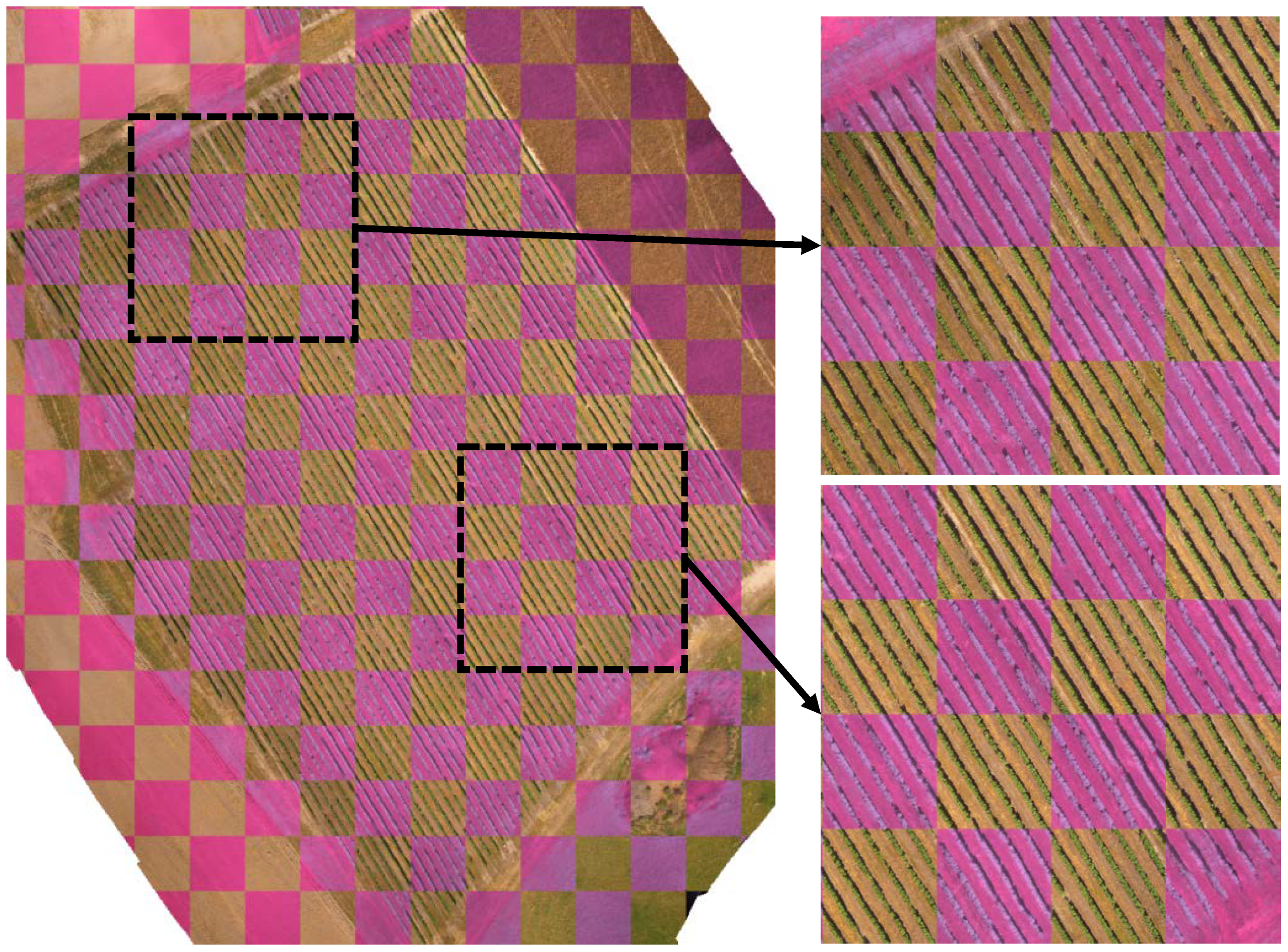
To evaluate the registration and depth map quality, we chose a chessboard test pattern. Figure 4 presents an example of visible and infrared orthophotos registration. As can be seen, the alignment between the two orthophotos is accurate. The registration of the depth map with the visible range also provides good results (Figure 6).
4.2. Training and Testing Architectures
In order to determine the best parameters for each deep learning architecture, four cross-optimizers with two loss functions were compared. Architectures were compiled using either the loss function “cross entropy” or “mean squared error”, and with one among the four optimizers: SGD [66], Adadelta [67], Adam [68], or Adamax [69]. Once the best parameters were defined for each architecture, a final fine-tuning was performed on the “learning rate” parameter to obtain the best results (to achieve a good model without overfitting). The best parameters found for each architecture are presented in Table 2.
For training the VddNet model, data from visible, near-infrared and depth maps were incorporated separately in the network inputs. For the other architectures, a multi-data matrix consists of five channels with a size of 256 × 256. The first three channels correspond to the visible spectrum, the 4th channel to the near-infrared data and the 5th channel to the depth map. Each multi-data matrix has a corresponding labelled matrix. Models training is an iterative process that is fixed at 30.000 epochs for each model. For each iteration, a batch of five multi-data matrices with their corresponding labelled matrices are randomly selected from the dataset and sent to feed the model. In order to check the convergence of the model, a test using validation data is performed each 10 iterations.
A qualitative study was conducted for determining the importance of depth map information. For this purpose, an experience was conducted by training the deep learning models with only multispectral data and with a combination of both (multispectral and depth maps). The comparison results are shown in Figures 7 and 8.
To test the deep learning models, test areas are segmented using a 256 × 256 sliding window (without overlap). For each position of the sliding window, the visible, near-infrared and depth maps are sent to the network inputs (respecting the data order for each architecture) in order to perform segmentation. The output of the networks is a matrix of size of 256 × 256 × 4. The results are saved after an application of the Argmax function. They are then stitched together to obtain the original size of the orthophoto tested data.
4.3. Segmentation Performance Measurements
Segmentation performance measurements are expressed in terms of recall, precision, F1-Score/Dice and accuracy (using Equations (1)–(5)) for each class (shadow, ground, healthy and diseased) at grapevine-scale. Grapevine-scale assessment was chosen because pixel-wise evaluation is not suitable for providing disease information. Moreover, imprecision of the ground truth, small surface of the disease and difference of deep learning segmentation results do not allow for a good evaluation of the different architectures, at pixel-wise. These measurements use a sliding window equivalent to the average size of a grapevine (in this study, approximatively 64 × 64 pixels). For each step of the sliding window, the class evaluated is the dominant class in the ground truth. The window is considered “true positive” if the dominant class is the same as the ground truth, otherwise it is a “false positive”. The confusion matrix is updated for each step. Finally, the score is given by
where TP, TN, FP and FN are the number of samples for “true positive”, “true negative”, “false positive” and “false negative”, respectively. Dice equation is defined by X (set of ground truth pixels) and Y (set of the classified pixels).
5. Discussion
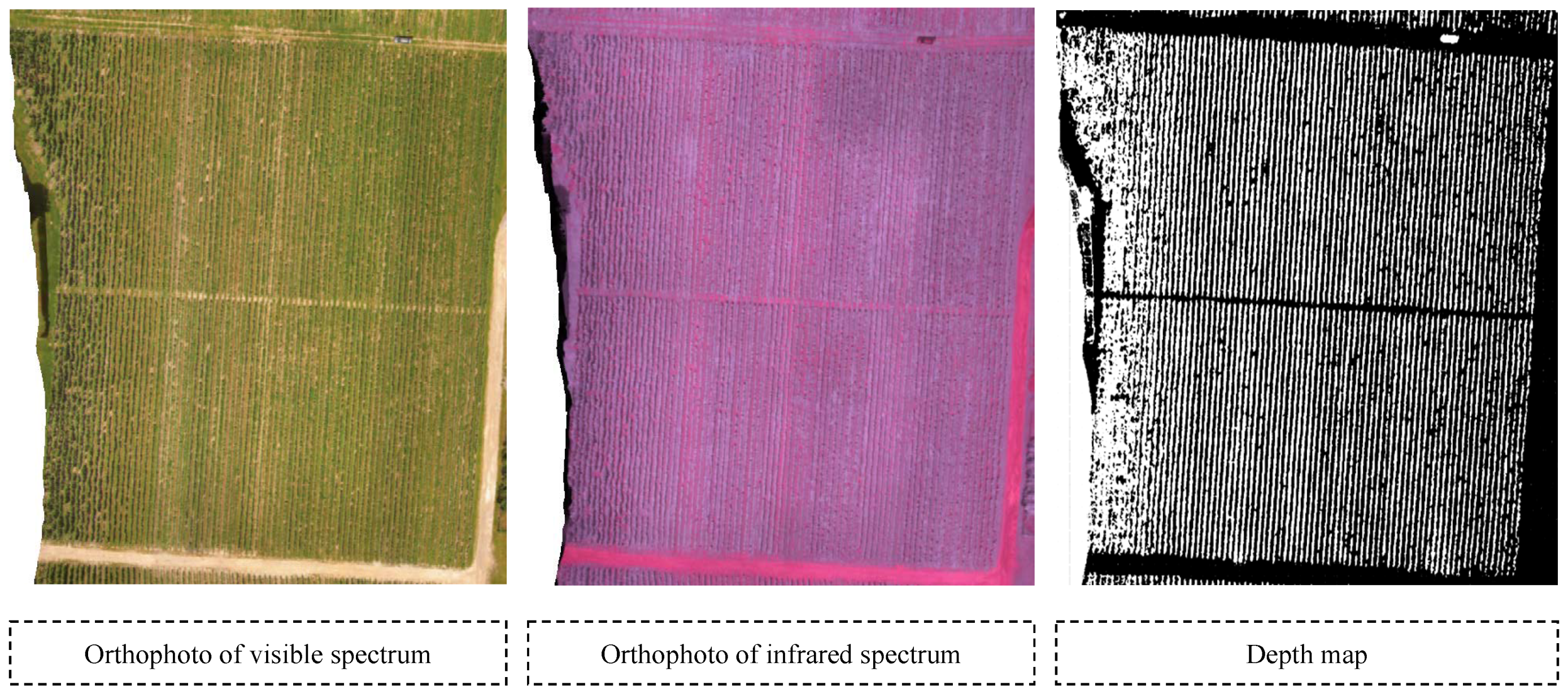
To validate the proposed vine disease detection system, it is necessary to evaluate and compare qualitative and quantitative results for each block of the whole system. For this purpose, several experiments were conducted at each step of the disease detection procedure. The first experience was carried out on the multimodal orthophotos registration. Figure 4 shows the obtained results. As can be seen, the continuity of the vinerows is highly accurate and the continuity is respected between the visible and infrared ranges. However, if image acquisition is incorrectly conducted, this results in many registration errors. To avoid these problems, two rules must be followed. The first one regards the overlapping between visible and infrared images acquired in the same position, which must be greater than 85%. The second rule is that the overlapping between each acquired image must be greater than 70%; this rule must be respected in both ranges. Non-compliance with the first rule affects the building of the registered infrared orthophoto. Indeed, this latter may present some black holes (this means that there are no data available to complete these holes). Non-compliance with the second rule affects the photogrammetry processing and the DSM model. This can lead to deformations in the orthophoto patterns (as can be seen on the left side of the visible and infrared orthophotos in Figure 5). In case the DSM model is impacted, the depth map automatically undergoes the same deformation (as can be seen in the depth map in Figure 5). The second quality evaluation is the building of the depth map (Figure 6). Despite the slight deformation in the left side of the parcel, the result of the depth map is consistent and well aligned with the visible orthophotos, and can be used in the segmentation process.
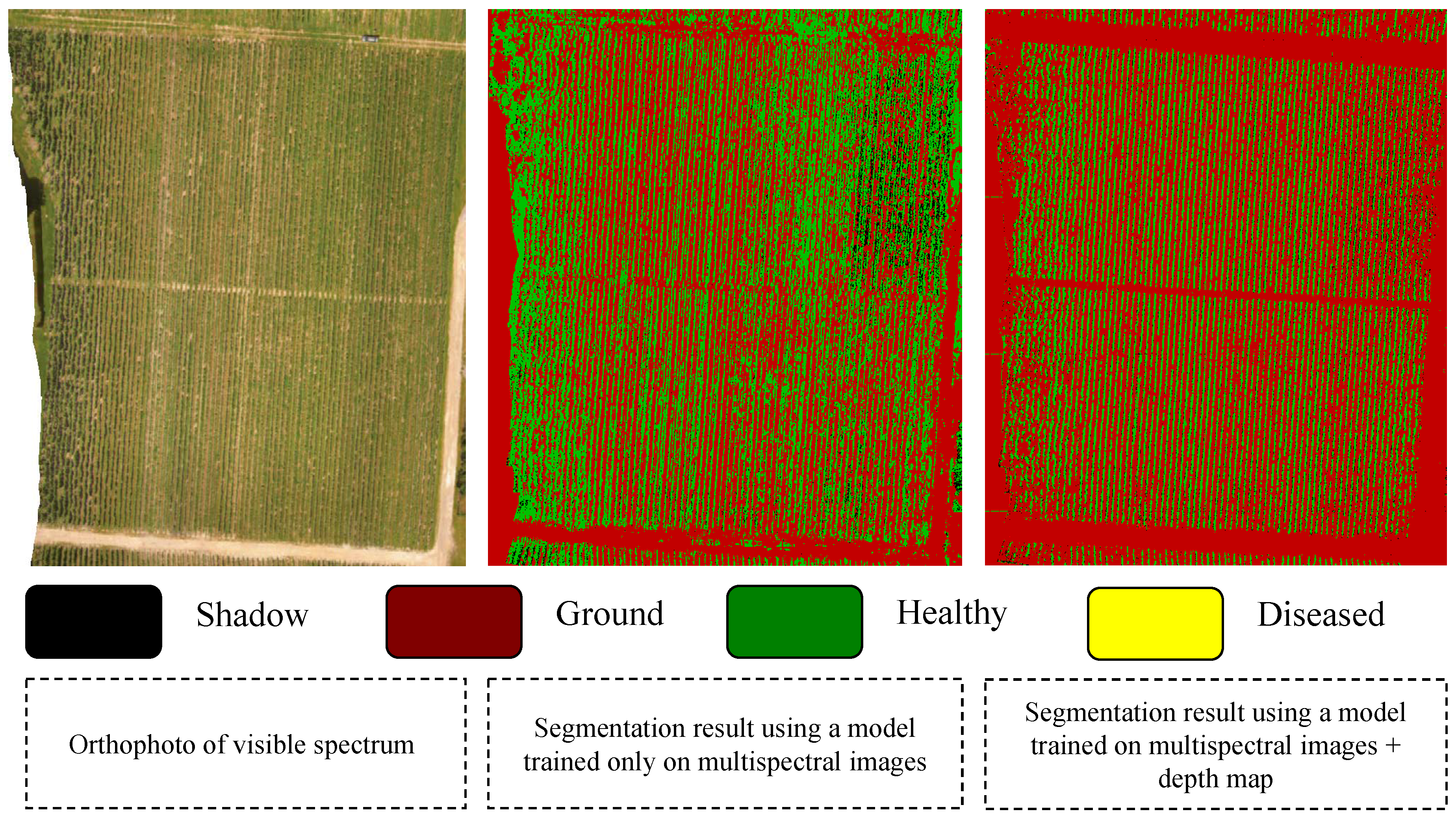
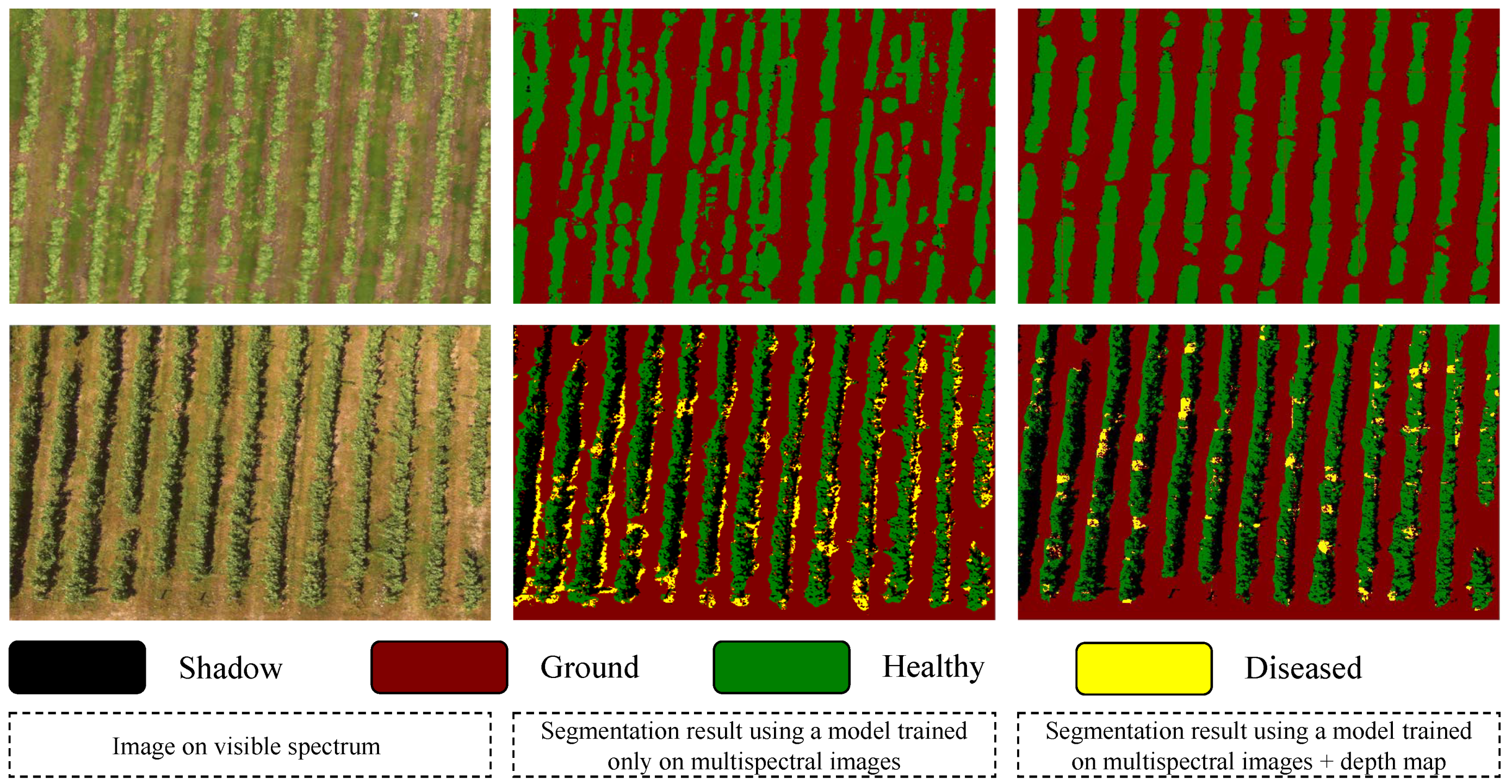
In order to assess the added value of depth map information, two training sessions were performed on the SegNet [33], U-Net [57], DeepLabv3+ [58] and PSPNet [59] networks. The first training session was conducted only on multispectral data, and the second one on multispectral data combined with depth map information. Figure 7 and Figure 8 illustrate the qualitative test results of the comparison between the two trainings. The left side of Figure 7 shows an example of a parcel with a green ground. The center of the figure presents the segmentation result of the SegNet model trained only on multispectral data. As can be seen, in some areas of the parcel, it is difficult to dissociate vinerows. The right side of the figure depicts the segmentation result of the SegNet model trained on multispectral data combined with depth map information. This result is better than the previous one and it can easily separate vinerows. This is due to additional depth map information that allows a better learning of the scene environment and distinction between classes. Figure 7 illustrates other examples realised under the same conditions as above. On the first row, we observe an area composed of green ground. The segmentation results using the first and second models are displayed in the centre and on the right side, respectively. We can notice in this example a huge confusion between ground and healthy vine classes. This is mainly due to the fact that the ground color is similar to the healthy vine one. This problem has been solved by adding depth map information in the second model, the result of which is shown on the right side. The second row of Figure 8 presents an example of a partially diseased area. The first segmentation result reveals the detection of the disease class on the ground. The brown color (original ground color) merged with a slight green color (grass color) on the ground confused the first model and led it to misclassifying the ground. This confusion does not exist in the second segmentation result (right side). From these results, it can be concluded that the second model learned that the diseased vine class could not be detected on “no-vine” when this one was trained on multispectral and depth map information. Based on these results, the following experiments were conducted using multispectral data and the depth map information.
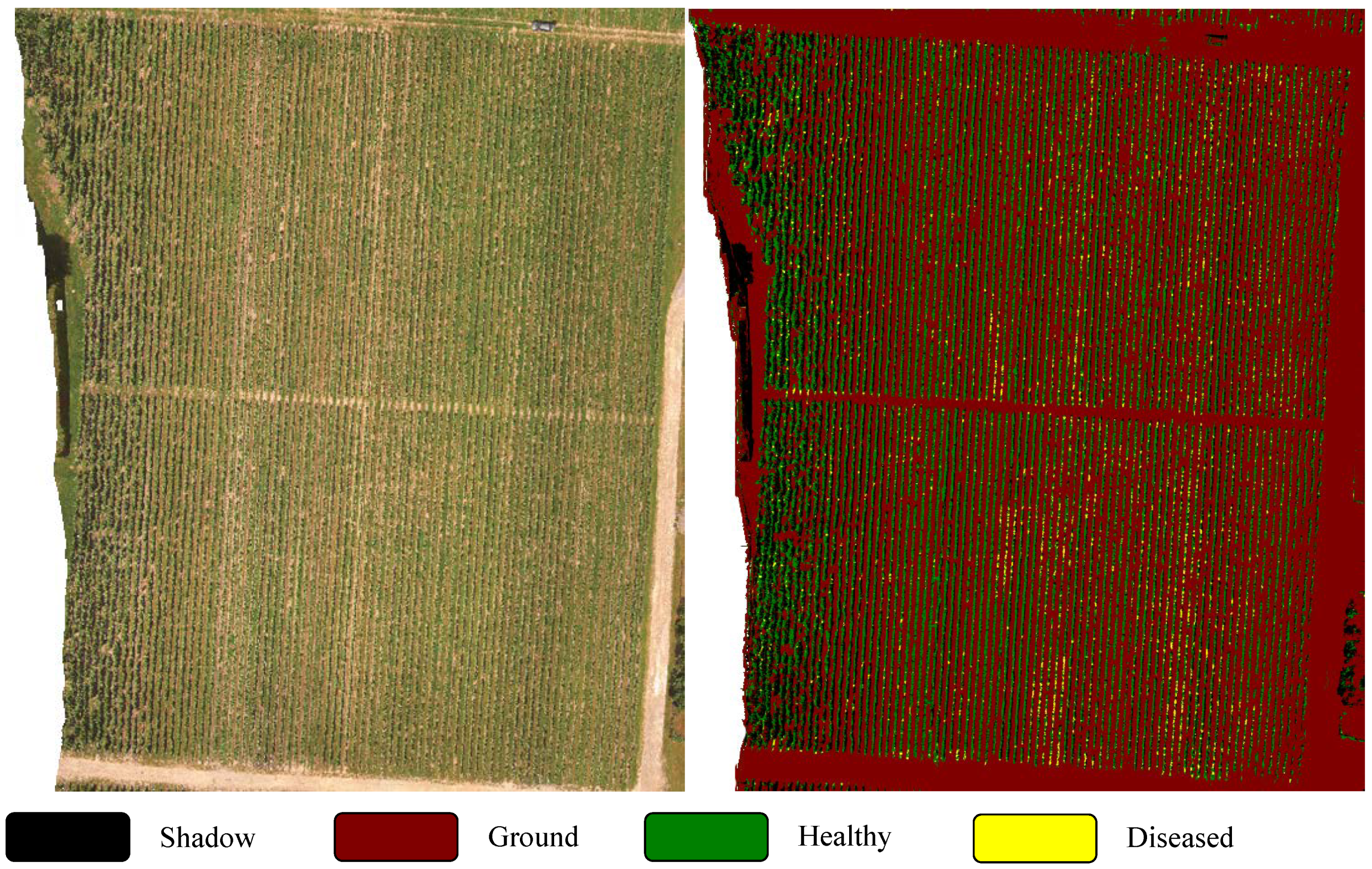
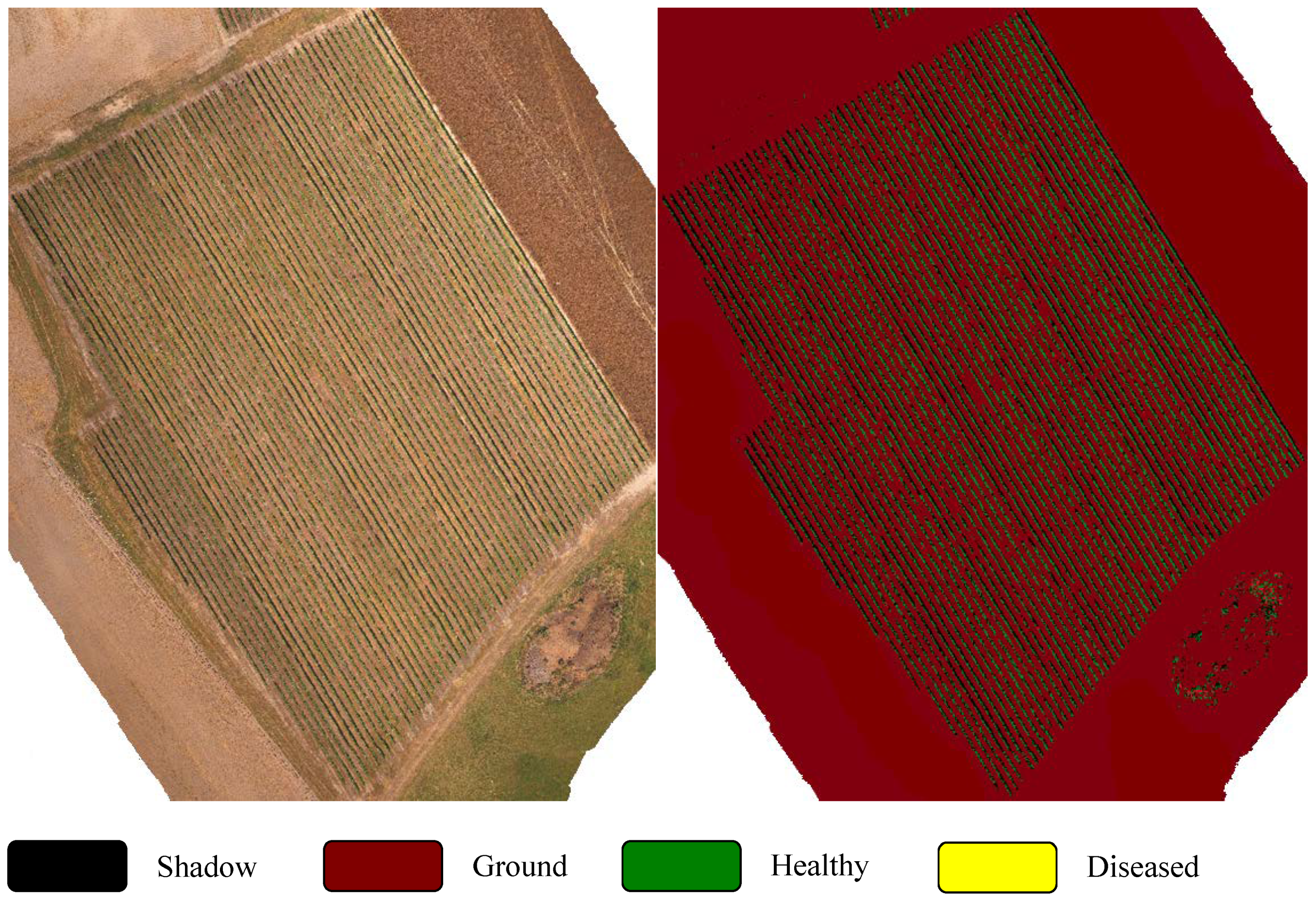
In order to validate the proposed architecture, a comparative study was conducted on the most well-known deep learning architectures, SegNet [33], U-Net [57], DeepLabv3+ [58] and PSPNet [59]. All architectures were trained and tested on the following classes: shadow, ground, healthy and diseased, with the same data (same training and test). Table 3 lists the segmentation results of the different architectures. The quantitative evaluations are based on the F1-score and the global accuracy. As can be seen, the shadow and ground classes have obtained an average scores of 94% and 95%, respectively, with all architectures. The high scores are due to the easy detection of these classes. The healthy class scored between 91% and 92% for VddNet, SegNet, U-Net and DeepLabv3+. However, PSPNet obtained the worst result of 73.96%, due to a strong confusion between the ground and healthy classes. PSPNet was unable to generate a good segmentation model although the training dataset was rich. The diseased vine class is the most important class in this study. VddNet obtained the best result for this class with a score of 92.59%, followed by SegNet with a score of 88.85%. The scores of the other architectures are 85.78%, 81.63% and 74.87% for U-Net, PSPNet and DeepLabv3+, respectively. VddNet achieved the best result because the feature extraction was performed separately. Indeed, in [21] it was proven that merging visible and infrared segmentations (with two separate trained models) provides a better detection than visible or infrared separately. The worst result of the diseased class was obtained with DeepLabv3+; this is due to a insensibility in the color variation. In fact, the diseased class can correspond to the yellow, brown or golden color and these colors are usually between the green color of healthy neighbour leaves. This situation led classifiers to be insensitive to this variation. The best global segmentation accuracy was achieved by VddNet, with an accuracy of 93.72%. This score can be observed on the qualitative results of Figure 9 and Figure 10. Figure 9 presents an orthophoto of a parcel (on the left side) partially contaminated with mildew. The right side shows the segmentation result by VddNet. It can be seen that it correctly detects the diseased areas. Figure 10 is an example of parcel without disease; here, VddNet also performs well in detecting true negatives.
6. Conclusions
The main goal of this study is to propose a new method that improves vine disease detection in UAV images. A new deep learning architecture for vine disease detection (VddNet), and automatic multispectral orthophotos registration have been proposed. UAV images in the visible and near-infrared spectra are the input data of the detection system for generating a disease map. UAV input images were aligned using an optimized multispectral registration algorithm. Aligned images were then used in the process of building registered orthophotos. During this process, a digital surface model (DSM) was generated to built a depth map. At the end, VddNet generated the disease map from visible, near-infrared and depth map data. The proposed method brought many benefits to the whole process. The automatic multispectral orthophotos registration provides high precision and fast processing compared to conventional procedures. A 3D processing enables the building of the depth map, which is relevant for the VddNet training and segmentation process. Depth map data reduce misclassification and confusion between close color classes. VddNet improves disease detection and global segmentation compared to the state-of-the-art architectures. Moreover, orthophotos are georeferenced with GNSS coordinates, making it easier to locate diseased vines for traitment. In future work, it would be interesting to acquire new multispectral channels to enhance disease detection and improve the VddNet architecture.
Author Contributions
M.K. and A.H. conceived and designed the method; M.K. implemented the method and performed the experiments; M.K., A.H. and R.C. discussed the results and revised the manuscript. All authors have read and agreed to the published version of the manuscript.
Funding
This research received no external funding.
Acknowledgments
This work is part of the VINODRONE project supported by the Region Centre-Val de Loire (France). We gratefully acknowledge Region Centre-Val de Loire for its support.
Conflicts of Interest
The authors declare no conflict of interest.
References
- Oerke, E.C. Crop losses to pests. J. Agric. Sci. 2006, 144, 31–43. [Google Scholar] [CrossRef]
- Patrício, D.I.; Rieder, R. Computer vision and artificial intelligence in precision agriculture for grain crops: A ystematic review. Comput. Electron. Agric. 2018, 153, 69–81. [Google Scholar] [CrossRef] [Green Version]
- Mogili, U.R.; Deepak, B.B. Review on Application of Drone Systems in Precision Agriculture. Procedia Comput. Sci. 2018, 133, 502–509. [Google Scholar] [CrossRef]
- Bellvert, J.; Zarco-Tejada, P.J.; Girona, J.; Fereres, E. Mapping crop water stress index in a ‘Pinot-noir’ vineyard: Comparing ground measurements with thermal remote sensing imagery from an unmanned aerial vehicle. Precis. Agric. 2014, 15, 361–376. [Google Scholar] [CrossRef]
- Mathews, A.J. Object-based spatiotemporal analysis of vine canopy vigor using an inexpensive unmanned aerial vehicle remote sensing system. J. Appl. Remote Sens. 2014, 8, 085199. [Google Scholar] [CrossRef]
- Vanino, S.; Pulighe, G.; Nino, P.; de Michele, C.; Bolognesi, S.F.; D’Urso, G. Estimation of evapotranspiration and crop coefficients of tendone vineyards using multi-sensor remote sensing data in a mediterranean environment. Remote Sens. 2015, 7, 14708–14730. [Google Scholar] [CrossRef] [Green Version]
- Bah, M.D.; Hafiane, A.; Canals, R. CRowNet: Deep Network for Crop Row Detection in UAV Images. IEEE Access 2020, 8, 5189–5200. [Google Scholar] [CrossRef]
- Dian Bah, M.; Hafiane, A.; Canals, R. Deep learning with unsupervised data labeling for weed detection in line crops in UAV images. Remote Sens. 2018, 10, 1690. [Google Scholar] [CrossRef] [Green Version]
- Tichkule, S.K.; Gawali, D.H. Plant diseases detection using image processing techniques. In Proceedings of the 2016 Online International Conference on Green Engineering and Technologies (IC-GET 2016), Coimbatore, India, 19 November 2016; pp. 1–6. [Google Scholar] [CrossRef]
- Pinto, L.S.; Ray, A.; Reddy, M.U.; Perumal, P.; Aishwarya, P. Crop disease classification using texture analysis. In Proceedings of the 2016 IEEE International Conference on Recent Trends in Electronics, Information and Communication Technology, RTEICT 2016—Proceedings, Bangalore, India, 20–21 May 2016; pp. 825–828. [Google Scholar] [CrossRef]
- MacDonald, S.L.; Staid, M.; Staid, M.; Cooper, M.L. Remote hyperspectral imaging of grapevine leafroll-associated virus 3 in cabernet sauvignon vineyards. Comput. Electron. Agric. 2016, 130, 109–117. [Google Scholar] [CrossRef] [Green Version]
- Junges, A.H.; Ducati, J.R.; Scalvi Lampugnani, C.; Almança, M.A.K. Detection of grapevine leaf stripe disease symptoms by hyperspectral sensor. Phytopathol. Mediterr. 2018, 57, 399–406. [Google Scholar] [CrossRef]
- di Gennaro, S.F.; Battiston, E.; di Marco, S.; Facini, O.; Matese, A.; Nocentini, M.; Palliotti, A.; Mugnai, L. Unmanned Aerial Vehicle (UAV)-based remote sensing to monitor grapevine leaf stripe disease within a vineyard affected by esca complex. Phytopathol. Mediterr. 2016, 55, 262–275. [Google Scholar] [CrossRef]
- Albetis, J.; Duthoit, S.; Guttler, F.; Jacquin, A.; Goulard, M.; Poilvé, H.; Féret, J.B.; Dedieu, G. Detection of Flavescence dorée grapevine disease using Unmanned Aerial Vehicle (UAV) multispectral imagery. Remote Sens. 2017, 9, 308. [Google Scholar] [CrossRef] [Green Version]
- Albetis, J.; Jacquin, A.; Goulard, M.; Poilvé, H.; Rousseau, J.; Clenet, H.; Dedieu, G.; Duthoit, S. On the potentiality of UAV multispectral imagery to detect Flavescence dorée and Grapevine Trunk Diseases. Remote Sens. 2019, 11, 23. [Google Scholar] [CrossRef] [Green Version]
- Al-Saddik, H.; Simon, J.; Brousse, O.; Cointault, F. Multispectral band selection for imaging sensor design for vineyard disease detection: Case of Flavescence Dorée. Adv. Anim. Biosci. 2017, 8, 150–155. [Google Scholar] [CrossRef] [Green Version]
- Al-Saddik, H.; Laybros, A.; Billiot, B.; Cointault, F. Using image texture and spectral reflectance analysis to detect Yellowness and Esca in grapevines at leaf-level. Remote Sens. 2018, 10, 618. [Google Scholar] [CrossRef] [Green Version]
- Al-saddik, H. Assessment of the optimal spectral bands for designing a sensor for vineyard disease detection: The case of ‘ Flavescence dorée ’. Precis. Agric. 2018. [Google Scholar] [CrossRef]
- Rançon, F.; Bombrun, L.; Keresztes, B.; Germain, C. Comparison of SIFT encoded and deep learning features for the classification and detection of esca disease in Bordeaux vineyards. Remote Sens. 2019, 11, 1. [Google Scholar] [CrossRef] [Green Version]
- Kerkech, M.; Hafiane, A.; Canals, R. Deep learning approach with colorimetric spaces and vegetation indices for vine diseases detection in UAV images. Comput. Electron. Agric. 2018, 155, 237–243. [Google Scholar] [CrossRef]
- Kerkech, M.; Hafiane, A.; Canals, R. Vine disease detection in UAV multispectral images using optimized image registration and deep learning segmentation approach. Comput. Electron. Agric. 2020, 174, 105446. [Google Scholar] [CrossRef]
- Kerkech, M.; Hafiane, A.; Canals, R.; Ros, F. Vine Disease Detection by Deep Learning Method Combined with 3D Depth Information; Lecture Notes in Computer Science; Springer International Publishing: Cham, Switzerland, 2020; Volume 12119, pp. 1–9. [Google Scholar] [CrossRef]
- Singh, V.; Misra, A.K. Detection of plant leaf diseases using image segmentation and soft computing techniques. Inf. Process. Agric. 2017, 4, 41–49. [Google Scholar] [CrossRef] [Green Version]
- Pilli, S.K.; Nallathambi, B.; George, S.J.; Diwanji, V. EAGROBOT - A robot for early crop disease detection using image processing. In Proceedings of the 2nd International Conference on Electronics and Communication Systems (ICECS 2015), Coimbatore, India, 26–27 February 2015; pp. 1684–1689. [Google Scholar] [CrossRef]
- Abbas, M.; Saleem, S.; Subhan, F.; Bais, A. Feature points-based image registration between satellite imagery and aerial images of agricultural land. Turk. J. Electr. Eng. Comput. Sci. 2020, 28, 1458–1473. [Google Scholar] [CrossRef]
- Ulabhaje, K. Survey on Image Fusion Techniques used in Remote Sensing. In Proceedings of the 2018 Second International Conference on Electronics, Communication and Aerospace Technology (ICECA), Coimbatore, India, 29–31 March 2018; pp. 1860–1863. [Google Scholar]
- Mukherjee, A.; Misra, S.; Raghuwanshi, N.S. A survey of unmanned aerial sensing solutions in precision agriculture. J. Netw. Comput. Appl. 2019, 148, 102461. [Google Scholar] [CrossRef]
- Xiong, Z.; Zhang, Y. A critical review of image registration methods. Int. J. Image Data Fusion 2010, 1, 137–158. [Google Scholar] [CrossRef]
- Unal, Z. Smart Farming Becomes even Smarter with Deep Learning—A Bibliographical Analysis. IEEE Access 2020, 8, 105587–105609. [Google Scholar] [CrossRef]
- Girshick, R.; Donahue, J.; Darrell, T.; Malik, J. Rich Feature Hierarchies for Accurate Object Detection and Semantic Segmentation. In Proceedings of the 2014 IEEE Conference on Computer Vision and Pattern Recognition, Columbus, OH, USA, 23–28 June 2014; Volume 1, pp. 580–587. [Google Scholar] [CrossRef] [Green Version]
- Bertinetto, L.; Valmadre, J.; Henriques, J.F.; Vedaldi, A.; Torr, P.H.S. Fully-Convolutional Siamese Networks for Object Tracking. In Lecture Notes in Computer Science (Including Subseries Lecture Notes in Artificial Intelligence and Lecture Notes in Bioinformatics); Elsevier B.V.: Amsterdam, The Netherlands, 2016; Volume 9914 LNCS, pp. 850–865. [Google Scholar] [CrossRef] [Green Version]
- He, K.; Zhang, X.; Ren, S.; Sun, J. Deep residual learning for image recognition. In Proceedings of the IEEE Computer Society Conference on Computer Vision and Pattern Recognition, Las Vegas, NV, USA, 27–30 June 2016; pp. 770–778. [Google Scholar] [CrossRef] [Green Version]
- Badrinarayanan, V.; Kendall, A.; Cipolla, R. SegNet: A Deep Convolutional Encoder-Decoder Architecture for Image Segmentation. IEEE Trans. Pattern Anal. Mach. Intell. 2017, 39, 2481–2495. [Google Scholar] [CrossRef]
- Polder, G.; Blok, P.M.; de Villiers, H.A.; van der Wolf, J.M.; Kamp, J. Potato virus Y detection in seed potatoes using deep learning on hyperspectral images. Front. Plant Sci. 2019, 10, 209. [Google Scholar] [CrossRef] [PubMed] [Green Version]
- Naseer, M.; Khan, S.; Porikli, F. Indoor Scene Understanding in 2.5/3D for Autonomous Agents: A Survey. IEEE Access 2019, 7, 1859–1887. [Google Scholar] [CrossRef]
- Sa, I.; Chen, Z.; Popovic, M.; Khanna, R.; Liebisch, F.; Nieto, J.; Siegwart, R. WeedNet: Dense Semantic Weed Classification Using Multispectral Images and MAV for Smart Farming. IEEE Robot. Autom. Lett. 2018, 3, 588–595. [Google Scholar] [CrossRef] [Green Version]
- Ren, X.; Du, S.; Zheng, Y. Parallel RCNN: A deep learning method for people detection using RGB-D images. In Proceedings of the 2017 10th International Congress on Image and Signal Processing, BioMedical Engineering and Informatics (CISP-BMEI 2017), Shanghai, China, 14–16 October 2017; pp. 1–6. [Google Scholar] [CrossRef]
- Gené-Mola, J.; Vilaplana, V.; Rosell-Polo, J.R.; Morros, J.R.; Ruiz-Hidalgo, J.; Gregorio, E. Multi-modal deep learning for Fuji apple detection using RGB-D cameras and their radiometric capabilities. Comput. Electron. Agric. 2019, 162, 689–698. [Google Scholar] [CrossRef]
- Bezen, R.; Edan, Y.; Halachmi, I. Computer vision system for measuring individual cow feed intake using RGB-D camera and deep learning algorithms. Comput. Electron. Agric. 2020, 172, 105345. [Google Scholar] [CrossRef]
- Aghi, D.; Mazzia, V.; Chiaberge, M. Local Motion Planner for Autonomous Navigation in Vineyards with a RGB-D Camera-Based Algorithm and Deep Learning Synergy. Machines 2020, 8, 27. [Google Scholar] [CrossRef]
- Burgos, S.; Mota, M.; Noll, D.; Cannelle, B. Use of very high-resolution airborne images to analyse 3D canopy architecture of a vineyard. Int. Arch. Photogramm. Remote Sens. Spat. Inf. Sci. ISPRS Arch. 2015, 40, 399–403. [Google Scholar] [CrossRef] [Green Version]
- Matese, A.; Di Gennaro, S.F.; Berton, A. Assessment of a canopy height model (CHM) in a vineyard using UAV-based multispectral imaging. Int. J. Remote Sens. 2017, 38, 2150–2160. [Google Scholar] [CrossRef]
- Weiss, M.; Baret, F. Using 3D Point Clouds Derived from UAV RGB Imagery to Describe Vineyard 3D Macro-Structure. Remote Sens. 2017, 9, 111. [Google Scholar] [CrossRef] [Green Version]
- Mahlein, A.K. Plant disease detection by imaging sensors—Parallels and specific demands for precision agriculture and plant phenotyping. Plant Dis. 2016, 100, 241–254. [Google Scholar] [CrossRef] [Green Version]
- Kaur, S.; Pandey, S.; Goel, S. Plants Disease Identification and Classification Through Leaf Images: A Survey. Arch. Comput. Methods Eng. 2019, 26, 507–530. [Google Scholar] [CrossRef]
- Saleem, M.H.; Potgieter, J.; Arif, K.M. Plant disease detection and classification by deep learning. Plants 2019, 8, 468. [Google Scholar] [CrossRef] [Green Version]
- Sandhu, G.K.; Kaur, R. Plant Disease Detection Techniques: A Review. In Proceedings of the 2019 International Conference on Automation, Computational and Technology Management (ICACTM 2019), London, UK, 24–26 April 2019; pp. 34–38. [Google Scholar] [CrossRef]
- Loey, M.; ElSawy, A.; Afify, M. Deep learning in plant diseases detection for agricultural crops: A survey. Int. J. Serv. Sci. Manag. Eng. Technol. 2020, 11, 41–58. [Google Scholar] [CrossRef]
- Schor, N.; Bechar, A.; Ignat, T.; Dombrovsky, A.; Elad, Y.; Berman, S. Robotic Disease Detection in Greenhouses: Combined Detection of Powdery Mildew and Tomato Spotted Wilt Virus. IEEE Robot. Autom. Lett. 2016, 1, 354–360. [Google Scholar] [CrossRef]
- Sharif, M.; Khan, M.A.; Iqbal, Z.; Azam, M.F.; Lali, M.I.U.; Javed, M.Y. Detection and classification of citrus diseases in agriculture based on optimized weighted segmentation and feature selection. Comput. Electron. Agric. 2018, 150, 220–234. [Google Scholar] [CrossRef]
- Ferentinos, K.P. Deep learning models for plant disease detection and diagnosis. Comput. Electron. Agric. 2018, 145, 311–318. [Google Scholar] [CrossRef]
- Argüeso, D.; Picon, A.; Irusta, U.; Medela, A.; San-Emeterio, M.G.; Bereciartua, A.; Alvarez-Gila, A. Few-Shot Learning approach for plant disease classification using images taken in the field. Comput. Electron. Agric. 2020, 175. [Google Scholar] [CrossRef]
- Jothiaruna, N.; Joseph Abraham Sundar, K.; Karthikeyan, B. A segmentation method for disease spot images incorporating chrominance in Comprehensive Color Feature and Region Growing. Comput. Electron. Agric. 2019, 165, 104934. [Google Scholar] [CrossRef]
- Pantazi, X.E.; Moshou, D.; Tamouridou, A.A. Automated leaf disease detection in different crop species through image features analysis and One Class Classifiers. Comput. Electron. Agric. 2019, 156, 96–104. [Google Scholar] [CrossRef]
- Abdulridha, J.; Ehsani, R.; Abd-Elrahman, A.; Ampatzidis, Y. A remote sensing technique for detecting laurel wilt disease in avocado in presence of other biotic and abiotic stresses. Comput. Electron. Agric. 2019, 156, 549–557. [Google Scholar] [CrossRef]
- Hu, W.j.; Fan, J.I.E.; Du, Y.X.; Li, B.S.; Xiong, N.N.; Bekkering, E. MDFC—ResNet: An Agricultural IoT System to Accurately Recognize Crop Diseases. IEEE Access 2020, 8, 115287–115298. [Google Scholar] [CrossRef]
- Ronneberger, O.; Fischer, P.; Brox, T. U-net: Convolutional networks for biomedical image segmentation. In Lecture Notes in Computer Science (Including Subseries Lecture Notes in Artificial Intelligence and Lecture Notes in Bioinformatics); Elsevier B.V.: Amsterdam, The Netherlands, 2015; Volume 9351, pp. 234–241. [Google Scholar] [CrossRef] [Green Version]
- Chen, L.C.; Zhu, Y.; Papandreou, G.; Schroff, F.; Adam, H. Encoder-Decoder with Atrous Separable Convolution for Semantic Image Segmentation. Pertanika J. Trop. Agric. Sci. 2018, 34, 137–143. [Google Scholar]
- Zhao, H.; Shi, J.; Qi, X.; Wang, X.; Jia, J. Pyramid scene parsing network. In Proceedings of the 30th IEEE Conference on Computer Vision and Pattern Recognition (CVPR 2017), Honolulu, HI, USA, 21–26 July 2017; Volume 2017, pp. 6230–6239. [Google Scholar] [CrossRef] [Green Version]
- Sermanet, P.; Eigen, D.; Zhang, X.; Mathieu, M.; Fergus, R.; LeCun, Y. Overfeat: Integrated recognition, localization and detection using convolutional networks. In Proceedings of the 2nd International Conference on Learning Representations (ICLR 2014), Conference Track Proceedings, Banff, AB, Canada, 14–16 April 2014. [Google Scholar]
- Liu, Y.; Chen, X.; Peng, H.; Wang, Z. Multi-focus image fusion with a deep convolutional neural network. Inf. Fusion 2017, 36, 191–207. [Google Scholar] [CrossRef]
- Adhikari, S.P.; Yang, H.; Kim, H. Learning Semantic Graphics Using Convolutional Encoder–Decoder Network for Autonomous Weeding in Paddy. Front. Plant Sci. 2019, 10, 1404. [Google Scholar] [CrossRef] [Green Version]
- Dunnhofer, M.; Antico, M.; Sasazawa, F.; Takeda, Y.; Camps, S.; Martinel, N.; Micheloni, C.; Carneiro, G.; Fontanarosa, D. Siam-U-Net: Encoder-decoder siamese network for knee cartilage tracking in ultrasound images. Med Image Anal. 2020, 60, 101631. [Google Scholar] [CrossRef]
- LeCun, Y.; Bottou, L.; Bengio, Y.; Haffner, P. Gradient-based learning applied to document recognition. Proc. IEEE 1998, 86, 2278–2323. [Google Scholar] [CrossRef] [Green Version]
- Dellana, R.; Roy, K. Data augmentation in CNN-based periocular authentication. In Proceedings of the 6th International Conference on Information Communication and Management (ICICM 2016), Hatfield, UK, 29–31 October 2016; pp. 141–145. [Google Scholar] [CrossRef]
- Hoffman, M.D.; Blei, D.M.; Wang, C.; Paisley, J. Stochastic variational inference. J. Mach. Learn. Res. 2013, 14, 1303–1347. [Google Scholar]
- Zeiler, M.D. ADADELTA: An Adaptive Learning Rate Method. arXiv 2012, arXiv:1212.5701. [Google Scholar]
- Kingma, D.P.; Ba, J.L. Adam: A method for stochastic optimization. In Proceedings of the 3rd International Conference on Learning Representations (ICLR 2015), Conference Track Proceedings, San Diego, CA, USA, 7–9 May 2015; pp. 1–15. [Google Scholar]
- Zeng, X.; Zhang, Z.; Wang, D. AdaMax Online Training for Speech Recognition. 2016, pp. 1–8. Available online: http://0-cslt-riit-tsinghua-edu-cn.brum.beds.ac.uk/mediawiki/images/d/df/Adamax_Online_Training_for_Speech_Recognition.pdf (accessed on 10 September 2020).
Figure 1.
The proposed vine disease detection system.

Figure 2.
The proposed orthophotos registration method.

Figure 3.
VddNet architecture.

Figure 4.
Qualitative results of orthophotos registration using a chessboard pattern.

Figure 5.
Qualitative results of orthophotos and depth map.

Figure 6.
Evaluation of the depth map alignment using a chessboard pattern.

Figure 7.
Difference between a SegNet model trained only on multispectral data and the same trained on multispectral data combined with depth map information. The presented example is on an orthophoto of a healthy parcel with a green ground.
Figure 7.
Difference between a SegNet model trained only on multispectral data and the same trained on multispectral data combined with depth map information. The presented example is on an orthophoto of a healthy parcel with a green ground.

Figure 8.
Difference between a SegNet model trained only on multispectral data and the same trained on multispectral data combined with depth map information. Two examples are presented here, the first row is an example on a healthy parcel with a green ground. The second one is an example on a partially diseased parcel with a brown ground.

Figure 9.
Qualitative result of VddNet on a parcel partially contaminated with mildew and with green ground. The visible orthophoto of the healthy parcel is in the left side, and its disease map in the right side.
Figure 9.
Qualitative result of VddNet on a parcel partially contaminated with mildew and with green ground. The visible orthophoto of the healthy parcel is in the left side, and its disease map in the right side.

Figure 10.
Qualitative result of VddNet on a healthy parcel with brown ground. The visible orthophoto of the healthy parcel is in the left side, and its disease map in the right side.
Figure 10.
Qualitative result of VddNet on a healthy parcel with brown ground. The visible orthophoto of the healthy parcel is in the left side, and its disease map in the right side.


Table 1.
The parameters used for the orthophotos building process in the Agisoft Metashape software.
Table 1.
The parameters used for the orthophotos building process in the Agisoft Metashape software.
| Sparse Point Cloud | |
| Accuracy: | High |
| Image pair selection: | Ground control |
| Constrain features by mask: | No |
| Maximum number of feature points: | 40,000 |
| Dense Point Cloud | |
| Quality: | High |
| Depth filtering: | Disabled |
| Digital Surface Model | |
| Type: | Geographic |
| Coordinate system: | WGS 84 (EPSG::4326) |
| Source data: | Dense cloud |
| Orthomosaic | |
| Surface: | DSM |
| Blending mode: | Mosaic |
Table 2.
The parameters used for the different deep learning architectures. LR means learning rate.
| Network | Base Model | Optimizer | Loss Function | LR | Learning Ate Decrease Parameters |
|---|---|---|---|---|---|
| SegNet | VGG-16 | Adadelta | Categorical cross entropy | 1.0 | rho = 0.95, epsilon = 1 × 10⁻⁷ |
| U-Net | VGG-11 | SGD | Categorical cross entropy | 0.1 | decay = 1 × 10⁻⁶, momentum = 0.9 |
| PSP-Net | ResNet-50 | Adam | Categorical cross entropy | 0.001 | beta1 = 0.9, beta2 = 0.999, epsilon = 1 × 10⁻⁷ |
| DeepLabv3+ | Xception | Adam | Categorical cross entropy | 0.001 | beta1 = 0.9, beta2 = 0.999, epsilon = 1 × 10⁻⁷ |
| VddNet | Parallel VGG-13 | SGD | Categorical cross entropy | 0.1 | decay = 1 × 10⁻⁶, momentum = 0.9 |
Table 3.
Quantitative results with measurement of recall (Rec.), precision (Pre.), F1-Score/Dice (F1/D.) and accuracy (Acc.) for the performances of VddNet, SegNet, U-Net, DeepLabv3+ and PSPNet networks, using multispectral and depth map data. Values are presented as a percentage.
Table 3.
Quantitative results with measurement of recall (Rec.), precision (Pre.), F1-Score/Dice (F1/D.) and accuracy (Acc.) for the performances of VddNet, SegNet, U-Net, DeepLabv3+ and PSPNet networks, using multispectral and depth map data. Values are presented as a percentage.
| Class name | Shadow | Ground | Healthy | Diseased | Total | ||||||||
|---|---|---|---|---|---|---|---|---|---|---|---|---|---|
| Measure | Rec. | Pre. | F1/D. | Rec. | Pre. | F1/D. | Rec. | Pre. | F1/D. | Rec. | Pre. | F1/D. | Acc. |
| VddNet | 94.88 | 94.89 | 94.88 | 94.84 | 95.11 | 94.97 | 87.96 | 94.84 | 91.27 | 90.13 | 95.19 | 92.59 | 93.72 |
| SegNet | 94.97 | 94.60 | 94.79 | 95.16 | 94.99 | 95.07 | 90.14 | 94.81 | 92.42 | 83.45 | 95.00 | 88.85 | 92.75 |
| U-Net | 95.09 | 94.70 | 94.90 | 94.99 | 95.07 | 95.03 | 89.09 | 94.74 | 91.83 | 78.27 | 94.90 | 85.78 | 90.69 |
| DeepLabV3+ | 94.90 | 94.68 | 94.79 | 95.21 | 94.90 | 95.06 | 88.78 | 95.16 | 91.86 | 61.78 | 94.98 | 74.87 | 88.58 |
| PSPNet | 95.07 | 94.25 | 94.66 | 94.94 | 87.29 | 90.95 | 60.54 | 95.04 | 73.96 | 71.70 | 94.75 | 81.63 | 84.63 |
© 2020 by the authors. Licensee MDPI, Basel, Switzerland. This article is an open access article distributed under the terms and conditions of the Creative Commons Attribution (CC BY) license (http://creativecommons.org/licenses/by/4.0/).
Share and Cite
MDPI and ACS Style
Kerkech, M.; Hafiane, A.; Canals, R. VddNet: Vine Disease Detection Network Based on Multispectral Images and Depth Map. Remote Sens. 2020, 12, 3305. https://0-doi-org.brum.beds.ac.uk/10.3390/rs12203305
AMA Style
Kerkech M, Hafiane A, Canals R. VddNet: Vine Disease Detection Network Based on Multispectral Images and Depth Map. Remote Sensing. 2020; 12(20):3305. https://0-doi-org.brum.beds.ac.uk/10.3390/rs12203305
Chicago/Turabian StyleKerkech, Mohamed, Adel Hafiane, and Raphael Canals. 2020. "VddNet: Vine Disease Detection Network Based on Multispectral Images and Depth Map" Remote Sensing 12, no. 20: 3305. https://0-doi-org.brum.beds.ac.uk/10.3390/rs12203305
Note that from the first issue of 2016, this journal uses article numbers instead of page numbers. See further details here.