Methodology of Processing Single-Strip Blocks of Imagery with Reduction and Optimization Number of Ground Control Points in UAV Photogrammetry


Abstract
:
1. Introduction
1.1. Related Works
1.2. Research Purpose
2. Materials
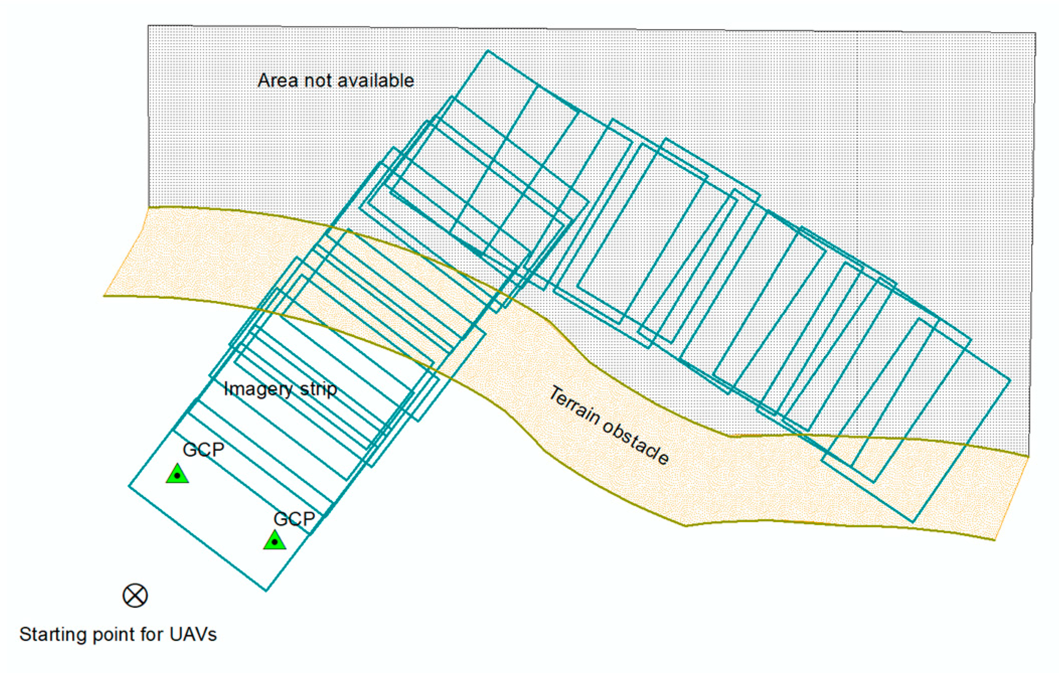
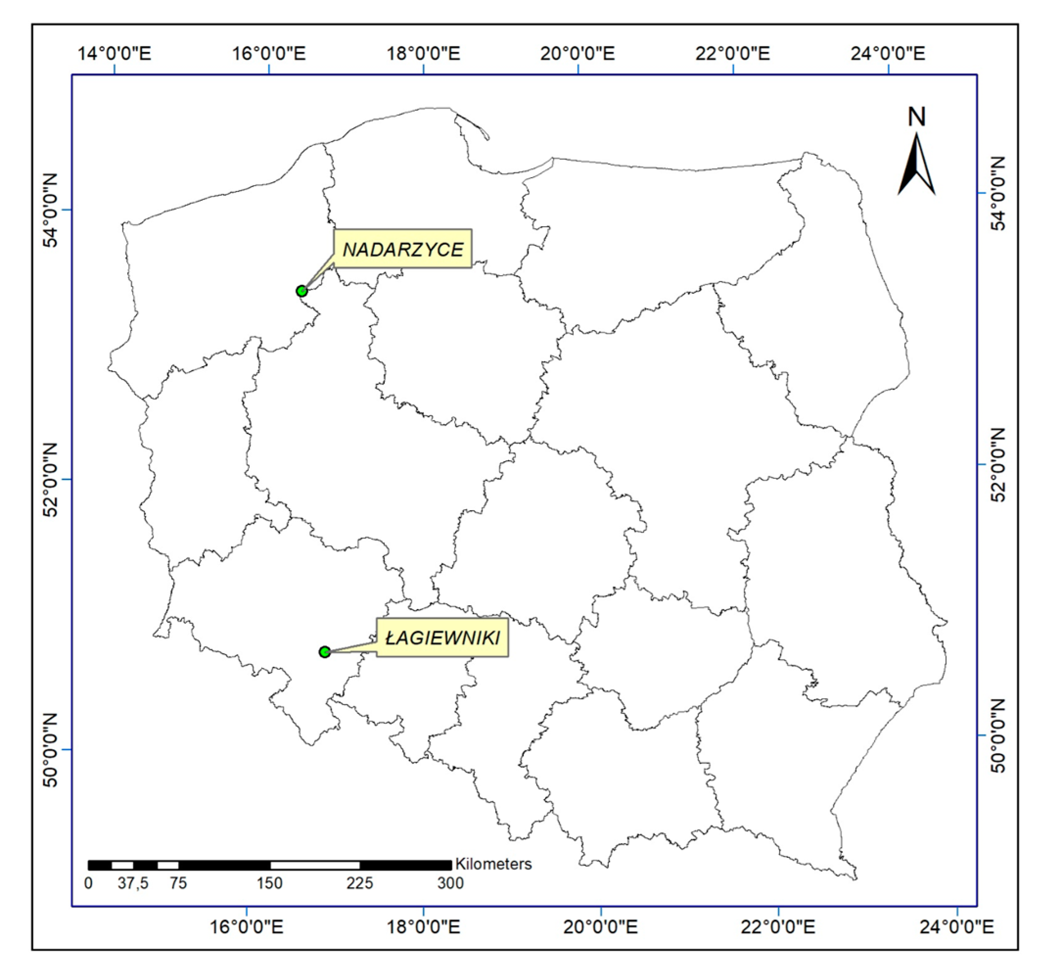
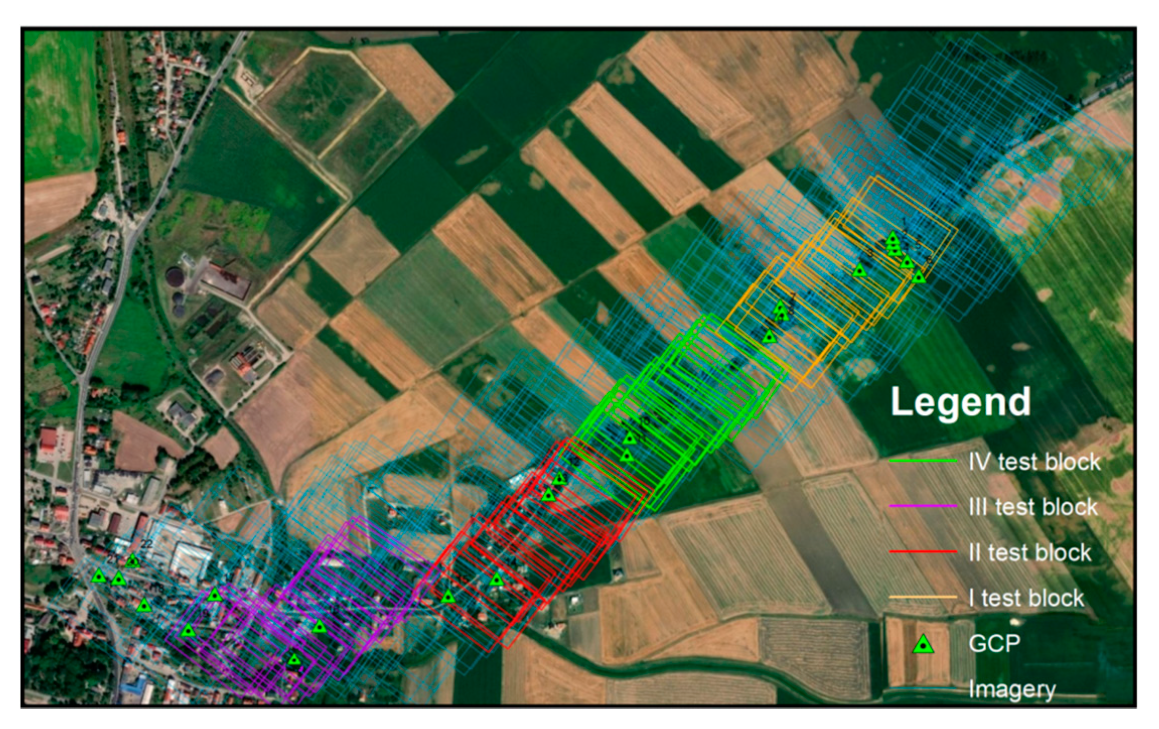
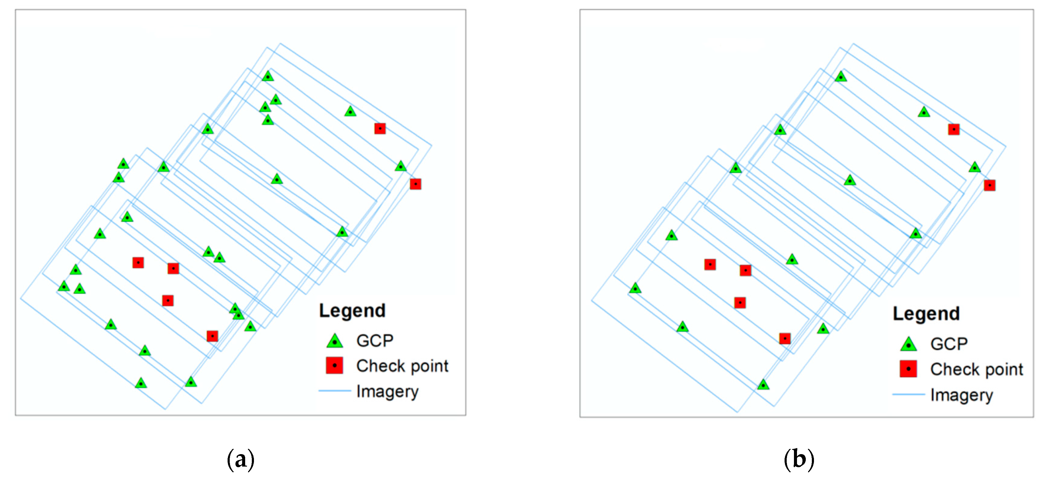
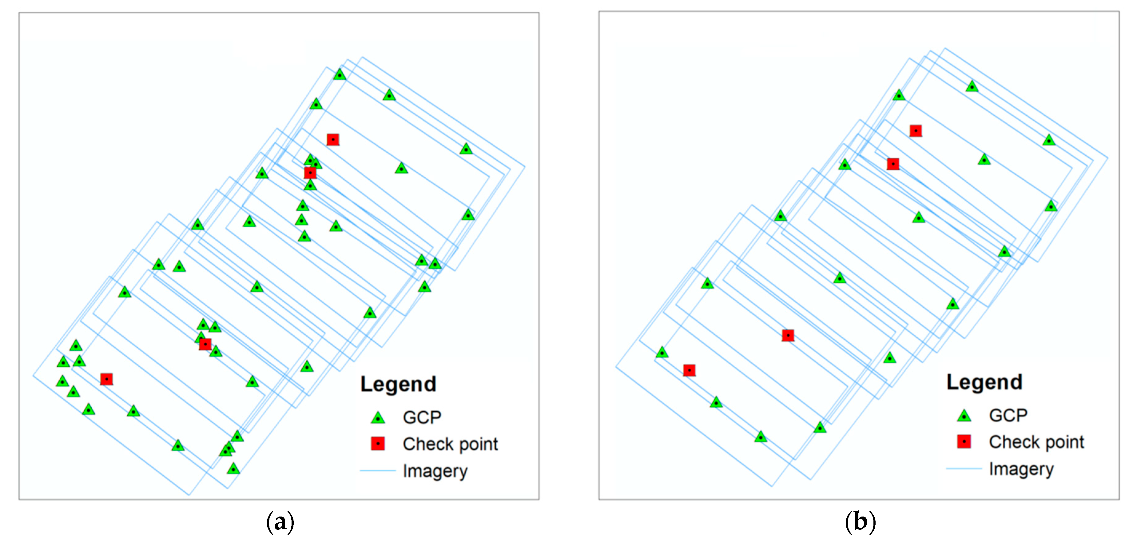
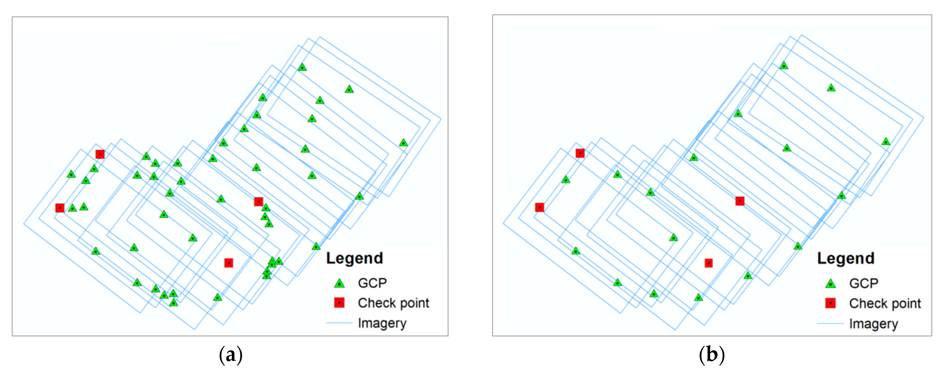
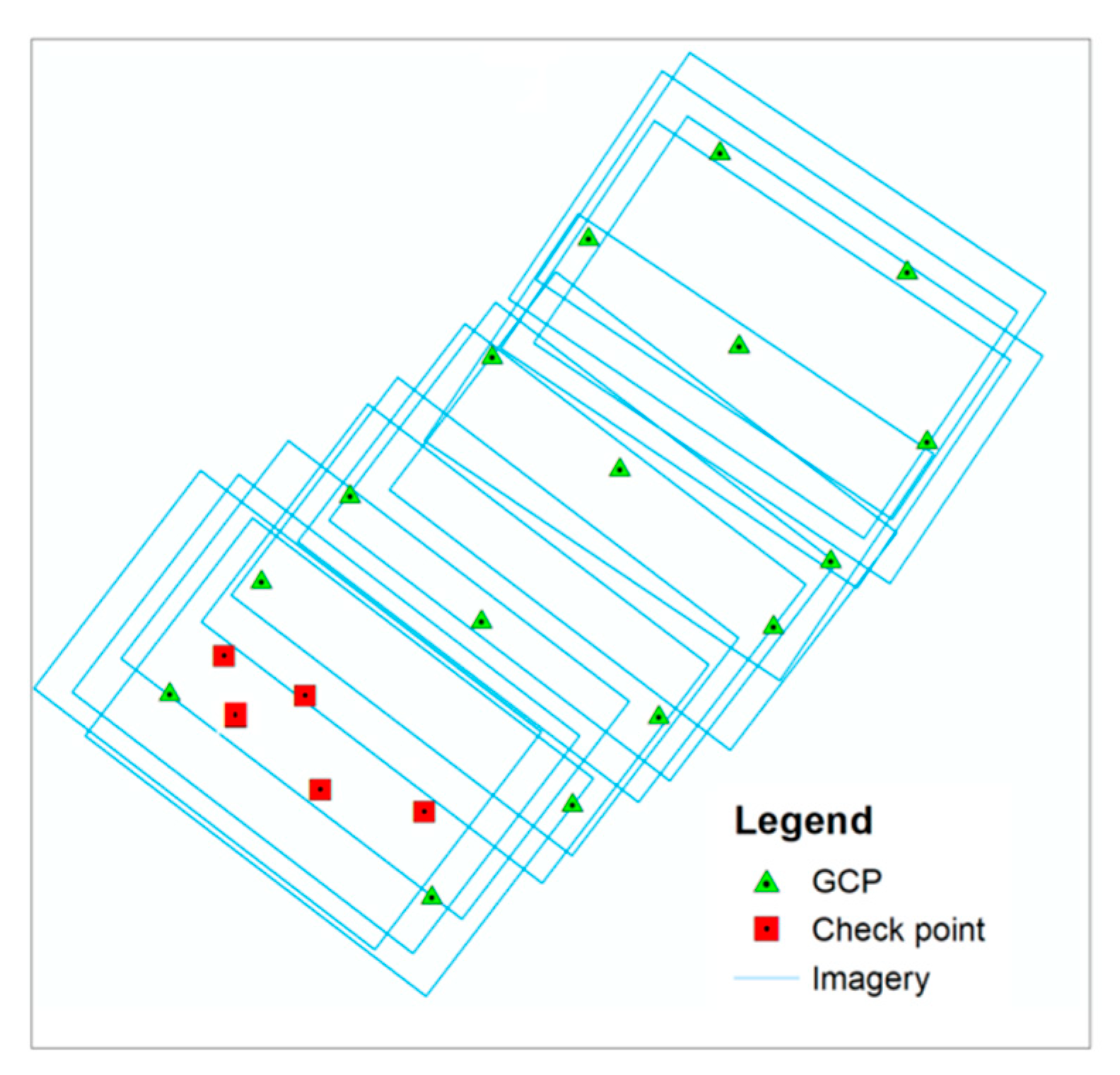
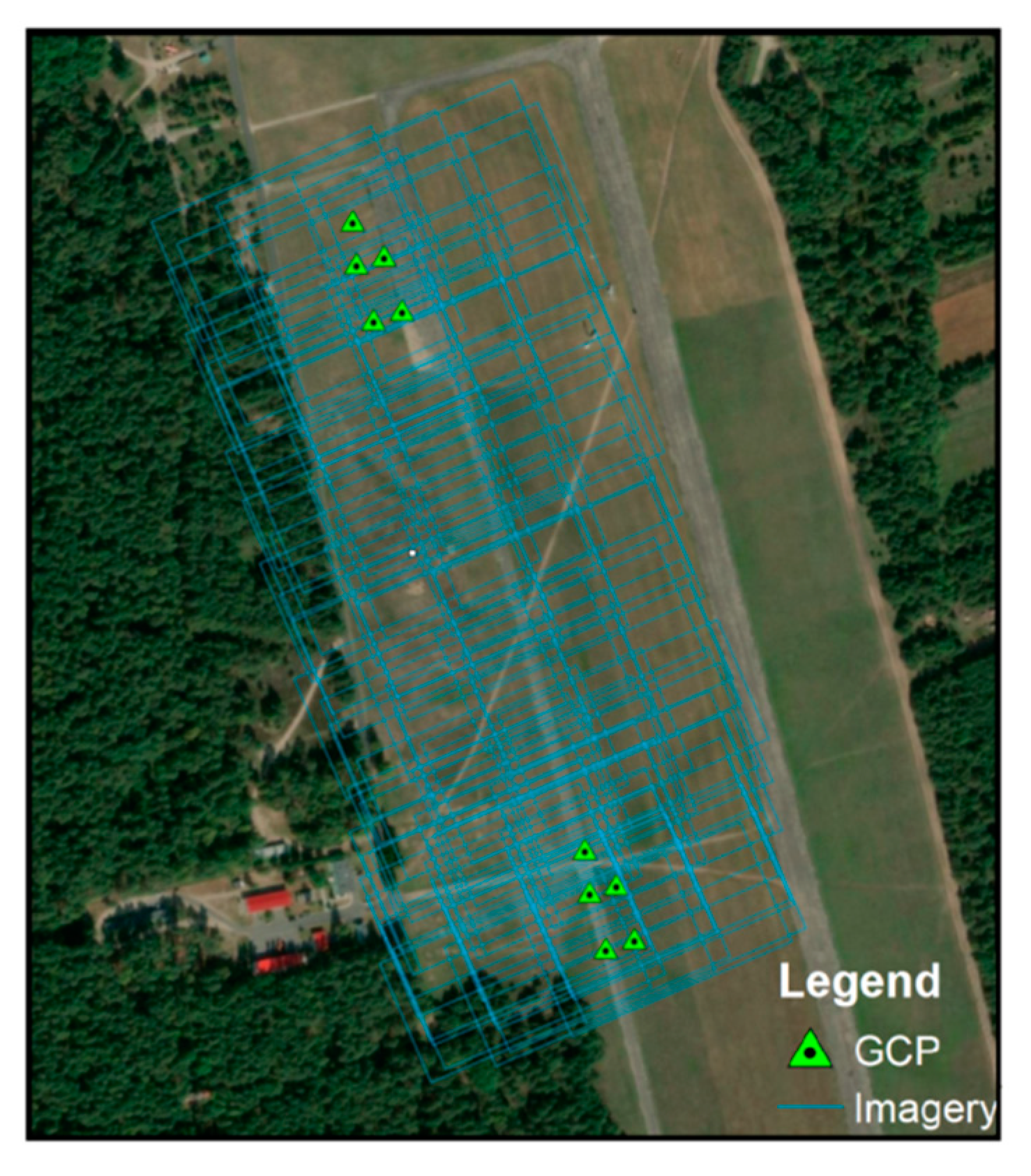
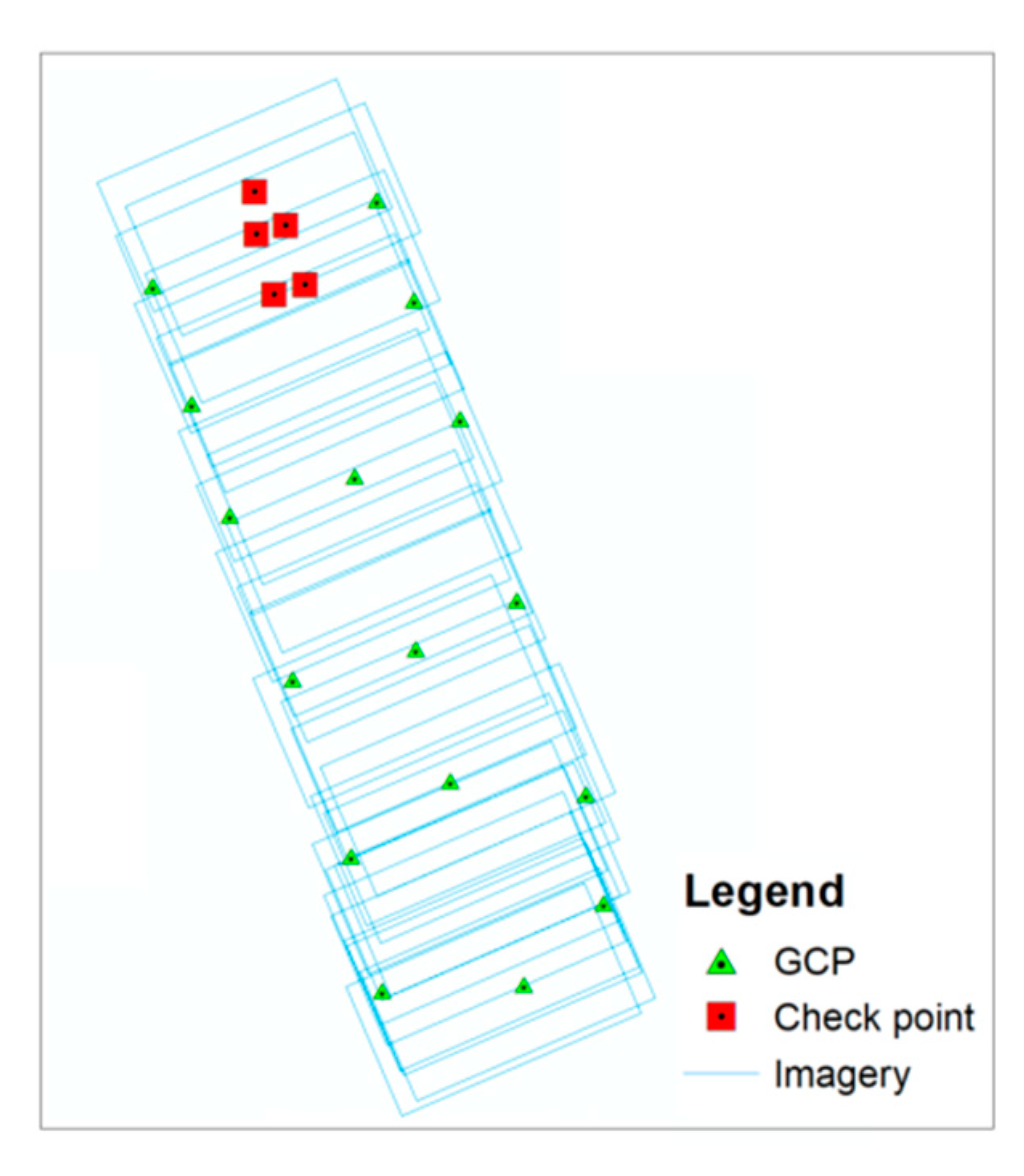
2.1. Study Area
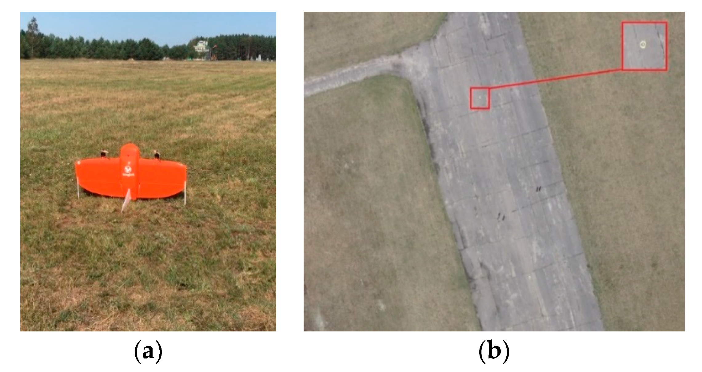
2.2. Description of Data Sets
2.3. Data Characteristics
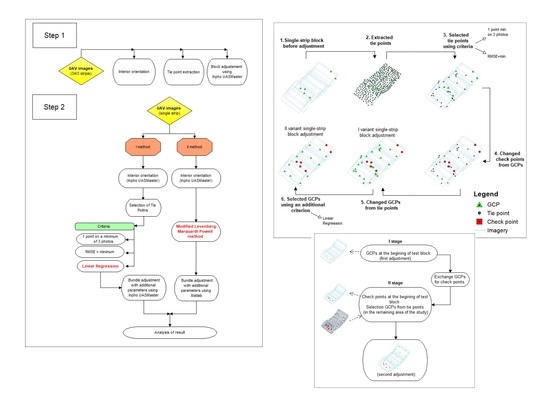
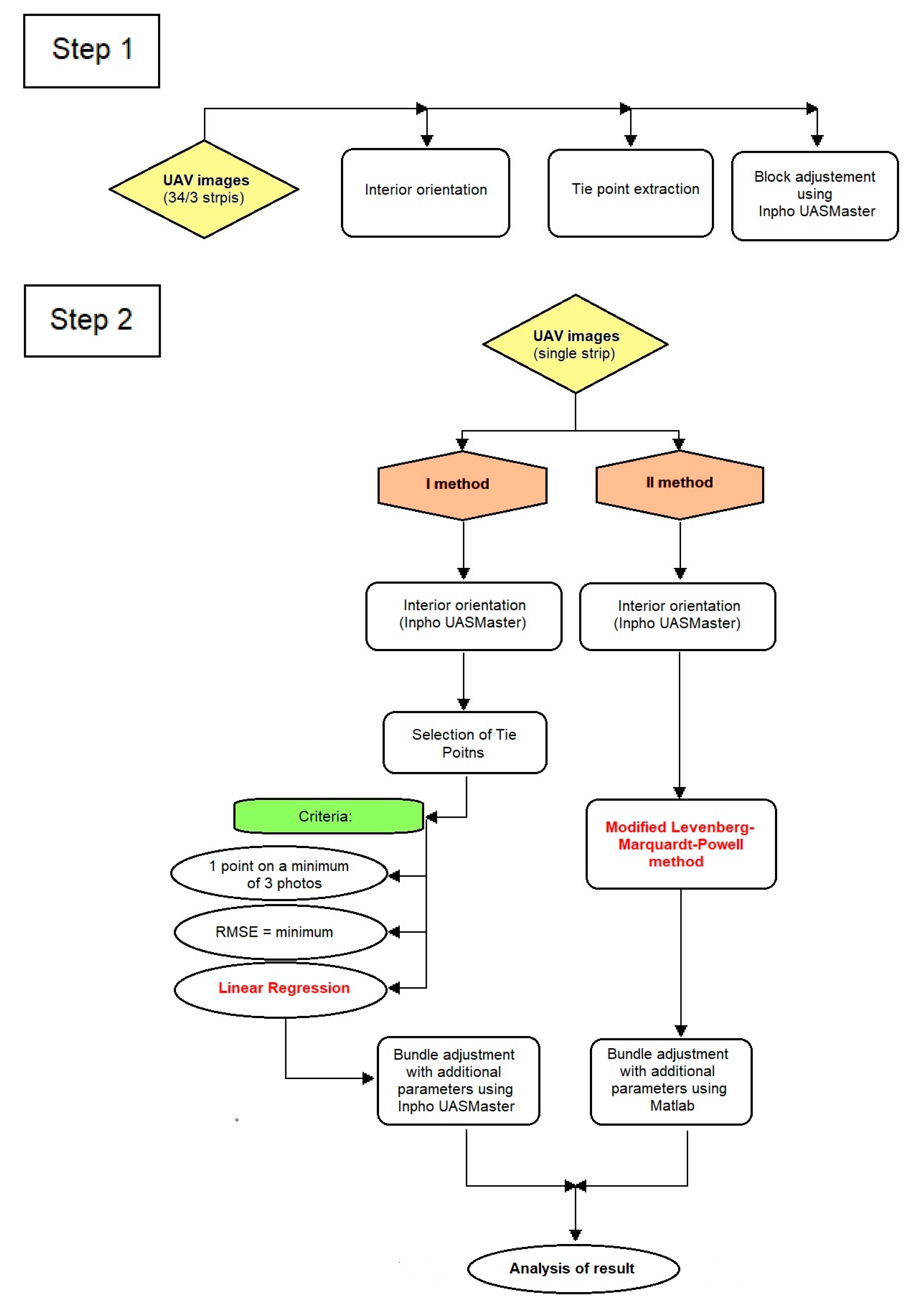
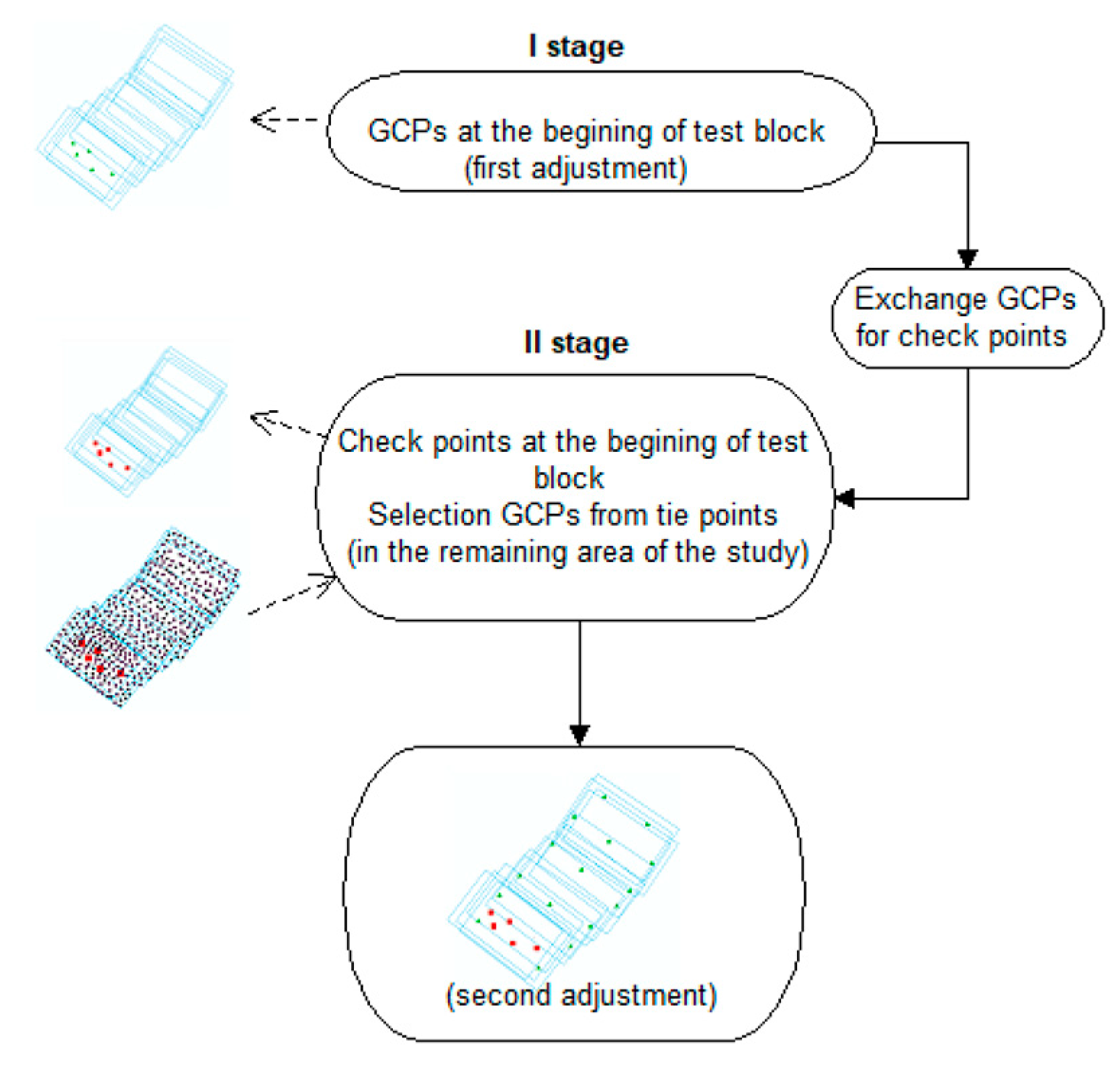
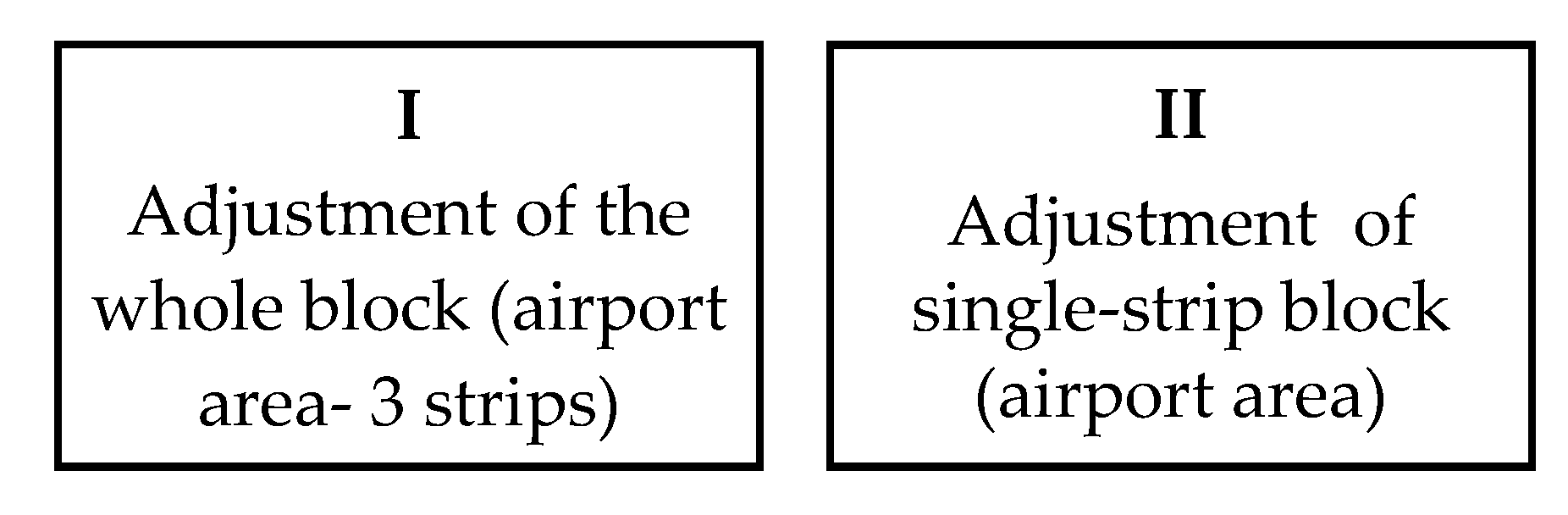
3. Methods
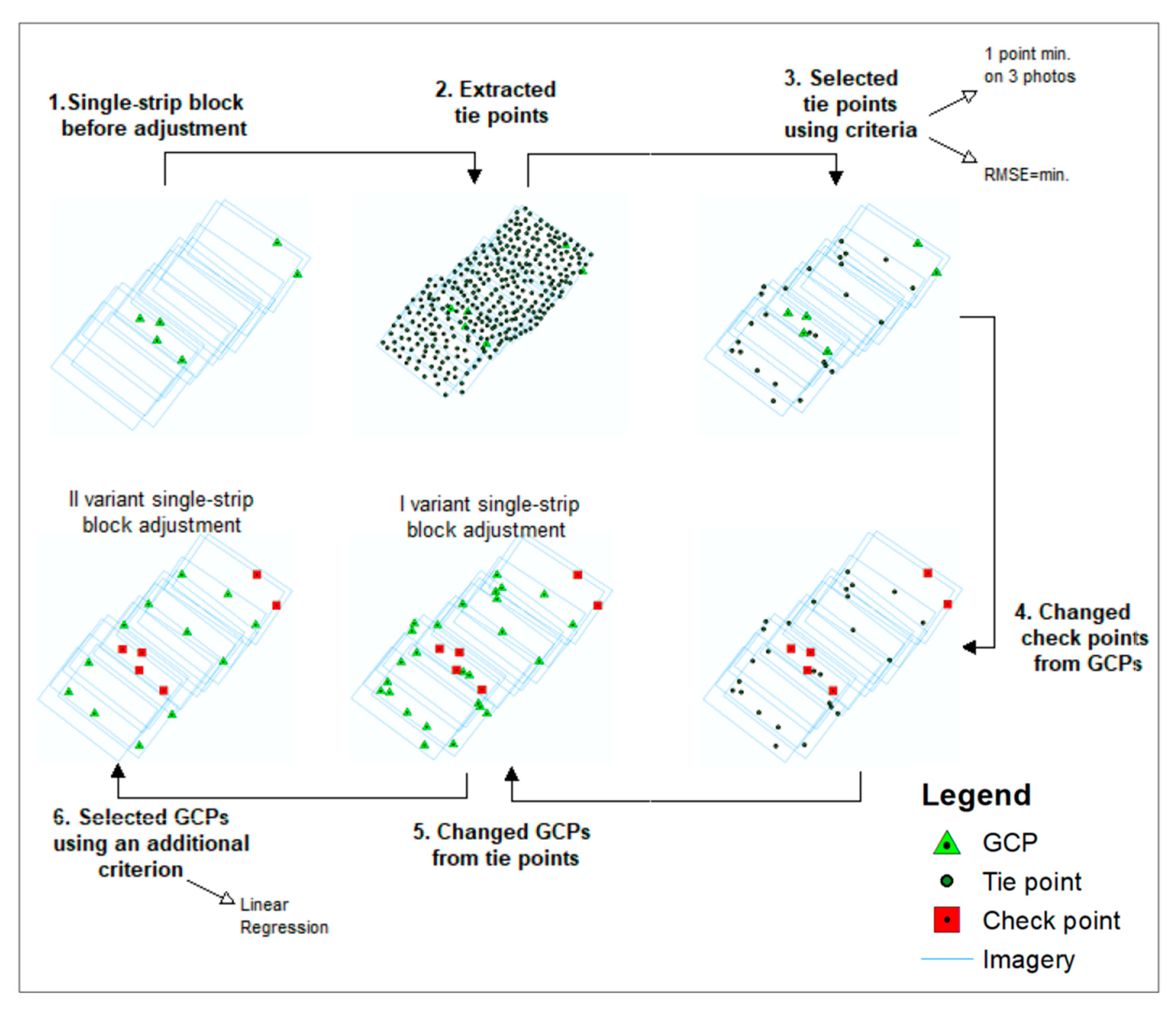
- One point on at least three images
- Points with the lowest mean square error (RMSE = minimum)
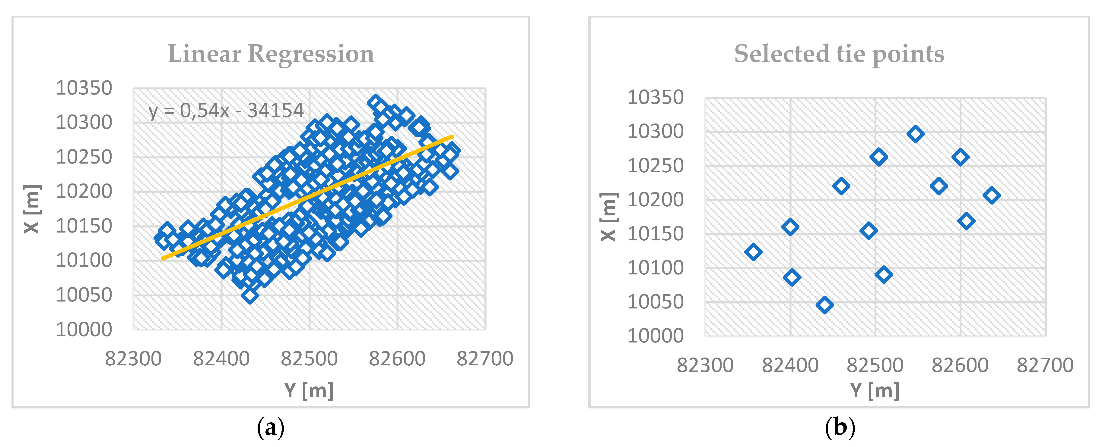
- Points evenly distributed within the area of development (linear regression method [61]).
3.1. Modified Linear Regression with Additional Parameters
3.2. Modified Bundle Adjustment with Additional Parameters
3.2.1. Problem-Specific Damping
3.2.2. Non-Linear Optimization
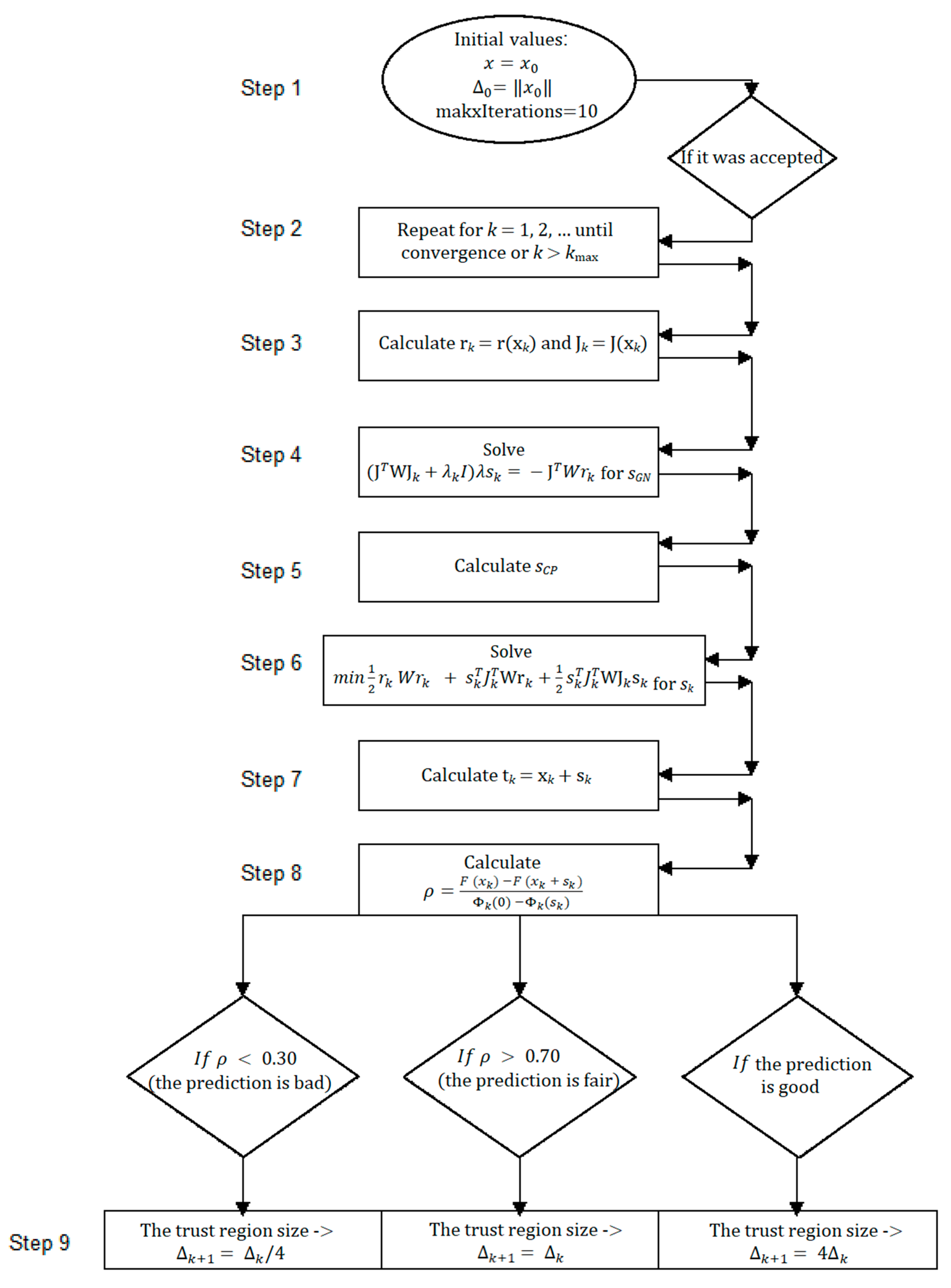
3.2.3. The Levenberg–Marquardt–Powell Method (Trust-Region)
3.2.4. Modified Powell Dogleg Method
4. Experiments and Results
4.1. Set I—Łagiewniki
4.1.1. Step I
Test block 0
4.1.2. Step II—I Method
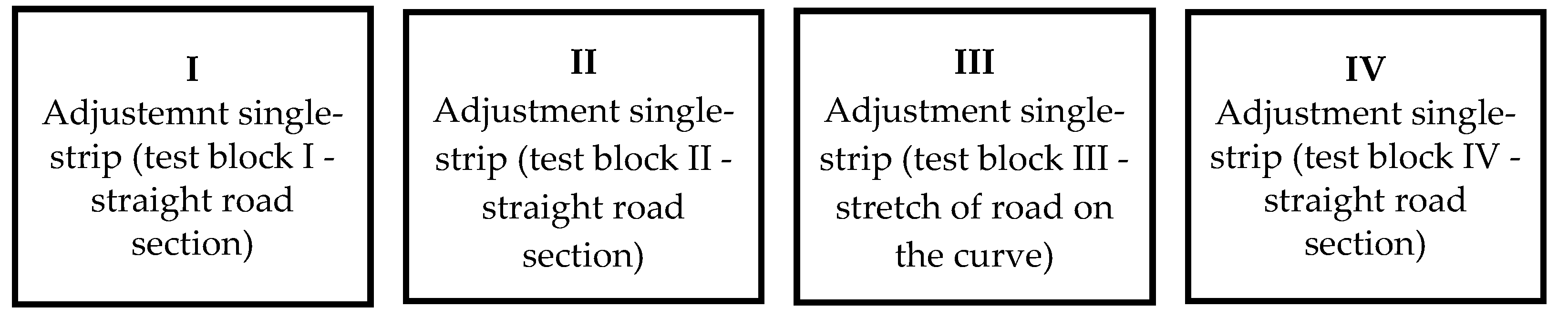
Test block I
Test block II
Test block III
- One point on minimum three images
- RMSE = minimum
- Linear regression
Test block IV
4.1.3. Step II—Method II
- Start with initial values x0 of the parameters and k0 = 0 (a maximum number of iterations = 10)
- Select an initial value of ∆0, such as ∆0 = ‖x0‖
- If ρ < 0.30 (the prediction is bad)—the trust region size -> ∆ + 1 = ∆k/4
- If ρ > 0.70 (the prediction is fair)—the trust region size -> ∆k + 1 = ∆k
- If the prediction is good the trust region size -> ∆k + 1 = ∆4k.
4.1.4. A Statistical Significance Test of Results—Data Set I
4.2. Set II—Nadarzyce
4.2.1. Step I
Test Block I
4.2.2. Step II—Method I
Test Block II
4.2.3. Step II—Method II
- Start with initial values x0 of the parameters and k0 = 0 (a maximum number of iterations = 10)
- Select an initial value of ∆0, such as ∆0 = ‖x0‖
- If ρ < 0.30 (the prediction is bad)—the trust region size -> ∆k+1 = ∆k/4
- If ρ > 0.70 (the prediction is fair)—the trust region size -> ∆k+1 = ∆k
4.2.4. A Statistical Significance Test of Results—Data Set II
4.2.5. Comparison of the Results of BBA using LMP Algorithm and with Precision Positioning Trajectory of UAV
5. Discussion
6. Conclusions
Author Contributions
Funding
Acknowledgments
Conflicts of Interest
Database
References
- Daakir, M.; Pierrot-Deseilligny, M.; Bosser, P.; Pichard, F.; Thom, C.; Rabot, Y.; Martin, O. Lightweight UAV with on-board photogrammetry and single-frequency GPS positioning for metrology applications. ISPRS J. Photogramm. Remote Sens. 2017, 127, 115–126. [Google Scholar] [CrossRef]
- Eling, C.; Wieland, M.; Hess, C.; Klingbeil, L.; Kuhlmann, H. Development and evaluation of a UAV based mapping system for remote sensing and surveying applications, The International Archives of the Photogrammetry, Remote Sensing and Spatial Information Sciences, Volume XL-1/W4. In Proceedings of the 2015 International Conference on Unmanned Aerial Vehicles in Geomatics, Toronto, ON, Canada, 30 August–2 September 2015. [Google Scholar]
- Colomina, I.; Molina, P. Unmanned aerial systems for photogrammetry and remote sensing: A review. ISPRSJ. Photogramm. Remote Sens. 2014, 92, 79–97. [Google Scholar] [CrossRef] [Green Version]
- Kędzierski, M.; Wierzbicki, D. Methodology of improvement of radiometric quality of images acquired from low altitudes. Measurement 2016, 92, 70–78. [Google Scholar] [CrossRef]
- Nex, F.; Remondino, F. UAV for 3D mapping applications: A review. Appl. Geomat. 2014, 6, 1–15. [Google Scholar] [CrossRef]
- Vacca, A.; Onishi, H. Drones: Military weapons, surveillance or mapping tools for environmental monitoring? The need for legal framework is required. Transp. Res. Procedia 2017, 25, 51–62. [Google Scholar] [CrossRef]
- Gonçalves, J.A.; Henriques, R. UAV photogrammetry for topographic monitoring of coast alareas. ISPRS J. Photogramm. Remote Sens. 2015, 104, 101–111. [Google Scholar] [CrossRef]
- Lin, Y.; Jiang, M.; Yao, Y.; Zhang, L.; Lin, J. Use of UAV oblique imaging for the detection of individual trees in residential environments. Urban For. Urban Green. 2015, 14, 404–412. [Google Scholar] [CrossRef]
- Jiang, S.; Jiang, W. Efficient structure from motion for oblique UAV images based on maximal spanning tree xpansion. ISPRSJ. Photogramm. Remote Sens. 2017, 132, 140–161. [Google Scholar] [CrossRef]
- Groos, A.R.; Bertschinger, T.J.; Kummer, C.M.; Erlwein, S.; Munz, L.; Philipp, A. The Potential of Low-Cost UAVs and Open-Source Photogrammetry Software for High-Resolution Monitoring of Alpine Glaciers: A Case Study from the Kanderfirn (Swiss Alps). Geosciences 2019, 9, 356. [Google Scholar] [CrossRef] [Green Version]
- Eisenbeiss, H. A mini Unmanned Aerial Vehicle (UAV): System overview and image acquisition. Int. Arch. Photogramm. Remote Sens. 2004, 36, 1–7. [Google Scholar]
- Berni, J.; Zarco-Tejada, P.; Suárez, L.; Fereres, E. Thermal and narrowband multispectral remote sensing for vegetation monitoring from an unmanned aerial vehicle. IEEE Trans. Geosci. Remote Sens. 2009, 47, 722–738. [Google Scholar] [CrossRef] [Green Version]
- Lin, Y.; Hyyppä, J.; Jaakkola, A. Mini-UAV-Borne LIDAR for Fine-Scale Mapping Geoscience and Remote Sensing Letters. IEEE Trans. Geosci. Remote Sens. 2011, 8, 426–430. [Google Scholar] [CrossRef]
- Lerma, J.; Navarro, S.; Cabrelles, M.; Villaverde, V. Terrestrial laser scanning and close range photogrammetry for 3D archaeological documentation: The Upper Palaeolithic cave of Parpall as a case study. J. Archaeol. Sci. 2010, 37, 499–507. [Google Scholar] [CrossRef]
- Reich, M.; Wiggenhagen, M.; Muhle, D. Filling the holes—Potential of UAV-based photogrammetric façade modeling. In Proceedings of the Tagungsband des 15, 3D-NordOst Workshops der GFaI, Berlin, Germany, 6–7 December 2012. [Google Scholar]
- Mesas-Carrascosa, F.; Rumbao, I.; Berrocal, J.; Porras, A. Positional Quality Assessment of Orthophotos Obtained from Sensors Onboard Multi-Rotor UAV Platforms. Sensors 2014, 14, 22394–22407. [Google Scholar] [CrossRef]
- Remondino, F.; Barazzetti, L.; Nex, F.; Scaioni, M.; Sarazzi, D. Uav photogrammetry for mapping and 3d modeling-current status and future perspectives. Int. Arch. Photogramm. Remote Sens. Spat. Inf. Sci. 2011, 38, C22. [Google Scholar] [CrossRef] [Green Version]
- Ahmad, A. Digital Mapping Using Low Altitude UAV. Pertanika J. Sci. Technol. 2011, 19, 51–58. [Google Scholar]
- Rozporządzenia Ministra Infrastruktury z dnia 25 czerwca 2003 w sprawie warunków, jakie powinny spełniać obiekty budowlane oraz naturalne w otoczeniu lotniska. Dziennik Ustaw, 8 August 2003. (In Polish)
- ICAO. Aeronautical Charts, Annex 4 to the Convention on International Civil Aviation, International Civil Aviation Organization, 9th ed.; ICAO: Montreal, QC, Canada, 2009; pp. 47–50. [Google Scholar]
- ICAO. Annex 14 to the Convention on International Civil Aviation Aerodromes—Aerodrome Desing and Operations, 7th ed.; ICAO: Montreal, QC, Canada, 2016; Available online: https://cockpitdata.com/Software/ICAO%20Annex%2014%20Volume%201%20%207th%20Edition%202016 (accessed on 12 October 2020).
- Rozporządzenie Ministra Infrastruktury z Dnia 20 lipca 2004 r. w Sprawie Wymagań dla Lądowisk. Dziennik Ustaw; 17 August 2004. Available online: http://isap.sejm.gov.pl/isap.nsf/DocDetails.xsp?id=WDU20041701791 (accessed on 12 October 2020). (In Polish)
- Decyzja Nr 348/Ministra Obrony Narodowej z dnia 28 grudnia 2016 r. w Sprawie Wprowadzenia do użytku w Lotnictwie Sił Zbrojnych Rzeczypospolitej Polskiej “Instrukcji Zarządzania Ruchem Lotniczym w Siłach Zbrojnych Rzeczypospolitej Polskiej” (IZRL-2017). Dziennik Urzędowy Ministra Obrony Narodowej. 30 December 2016. 25. Available online: https://www.infor.pl/akt-prawny/U23.2016.081.0000220,decyzja-nr-348mon-ministra-obrony-narodowej-w-sprawie-wprowadzenia-do-uzytku-w-lotnictwie-sil-zbrojnych-rzeczypospolitej-polskiej-instrukcji-zarzadzania-ruchem-lotniczym-w-silach-zbrojnych-rzeczypospo.html (accessed on 12 October 2020). (In Polish).
- He, F.; Habib, A.; Al-Rawabdeh, A. Planar constraints for an improved uav-image-based dense point cloud generation. Int. Arch. Photogramm. Remote Sens. Spat. Inf. Sci. 2015, 40, 269. [Google Scholar] [CrossRef] [Green Version]
- Lari, Z.; Al-Rawabdeh, A.; He, F.; Habib, A.; El-Sheimya, N. Region-based 3D surface reconstruction using images acquired by low-cost unmanned aerial systems. ISPRS-Int. Arch. Photogramm. Remote Sens. Spat. Inf. Sci. 2015, 40, 167–173. [Google Scholar] [CrossRef] [Green Version]
- He, F.; Habib, A. Automated Relative Orientation of UAV-Based Imagery in the Presence of Prior Information for the Flight Trajectory. Photogramm. Eng. Remote Sens. 2016, 82, 879–891. [Google Scholar] [CrossRef]
- Gomez, C.; Purdie, H. UAV-based photogrammetry and geocomputing for hazards and disaster risk monitoring—A review. Geoenviron. Disast. 2016, 3, 23. [Google Scholar] [CrossRef] [Green Version]
- Tsouros, D.C.; Bibi, S.; Sarigiannidis, P.G. A Review on UAV-Based Applications for Precision Agriculture. Information 2019, 10, 349. [Google Scholar] [CrossRef] [Green Version]
- Tao, W.; Lei, Y. UAV aerotriangulation with flight-control data support. In Proceedings of the 2011 Second International Conference on Mechanic Automation and Control Engineering, Hohhot, China, 15–17 July 2011; pp. 2801–2804. [Google Scholar]
- Przybilla, H.J.; Bäumker, M.; Luhmann, T.; Hastedt, H.; Eilers, M. Interaction between direct georeferencing, control point configuration and camera self-calibration for rtk-based uav photogrammetry. Int. Arch. Photogramm. Remote Sens. Spat. Inf. Sci. 2020, 43, 485–492. [Google Scholar] [CrossRef]
- Luhmann, T.; Robson, S. Close Range Photogrammetry: Principles, Methods and Applications, Cdr ed.; Whittles Publishing: Dunbeath, UK, 2011. [Google Scholar]
- Fryer, J.; Mitchell, H.; Chandler, J. Applications of 3D Measurement from Images; Whittles Publishing: Dunbeath, UK, 2007; p. 312. [Google Scholar]
- DeWitt, B.A.; Wolf, P.R. Elements of Photogrammetry (with Applications in GIS), 3rd ed.; McGraw-Hill Higher Education: New York, NY, USA, 2000. [Google Scholar]
- Harwin, S.; Lucieer, A. Assessing the accuracy of georeferenced point clouds produced via multi-view stereopsis from Unmanned Aerial Vehicle (UAV) imagery. Remote Sens. 2012, 4, 1573–1599. [Google Scholar] [CrossRef] [Green Version]
- Mancini, F.; Dubbini, M.; Gattelli, M.; Stecchi, F.; Fabbri, S.; Gabbianelli, G. Using Unmanned Aerial Vehicles (UAV) for High-Resolution Reconstruction of Topography: The Structure from Motion Approach on Coastal Environments. Remote Sens. 2013, 5, 6880–6898. [Google Scholar] [CrossRef] [Green Version]
- Yang, H.; Li, H.; Gong, Z.; Dai, W.; Lu, S. Relations between the Number of GCPs and Accuracy of UAV Photogrammetry in the Foreshore of the Sandy Beach. J. Coast. Res. 2020, 95, 1372–1376. [Google Scholar] [CrossRef]
- Saponaro, M.; Tarantino, E.; Reina, A.; Furfaro, G.; Fratino, U. Assessing the Impact of the Number of GCPS on the Accuracy of Photogrammetric Mapping from UAV Imagery. Baltic Surv. 2019, 10, 43–51. [Google Scholar]
- Tmušić, G.; Manfreda, S.; Aasen, H.; James, M.R.; Gonçalves, G.; Ben Dor, E.; Brook, A.; Polinova, M.; Arranz, J.J.; Mészáros, J.; et al. Current Practices in UAS-based Environmental Monitoring. Remote Sens. 2020, 12, 1001. [Google Scholar] [CrossRef] [Green Version]
- Tahar, K.N. An evaluation on different number of ground control points in unmanned aerial vehicle photogrammetric block. Int. Arch. Photogramm. Remote Sens. Spat. Inf. Sci. 2013, 40, 93–98. [Google Scholar] [CrossRef] [Green Version]
- Shahbazi, M.; Sohn, G.; Théau, J.; Menard, P. Development and evaluation of a UAV-photogrammetry system for precise 3D environmental modeling. Sensors 2015, 15, 27493–27524. [Google Scholar] [CrossRef] [Green Version]
- Oniga, V.-E.; Breaban, A.-I.; Pfeifer, N.; Chirila, C. Determining the Suitable Number of Ground Control Points for UAS Images Georeferencing by Varying Number and Spatial Distribution. Remote Sens. 2020, 12, 876. [Google Scholar] [CrossRef] [Green Version]
- Yu, J.J.; Kim, D.W.; Lee, E.J.; Son, S.W. Determining the Optimal Number of Ground Control Points for Varying Study Sites through Accuracy Evaluation of Unmanned Aerial System-Based 3D Point Clouds and Digital Surface Models. Drones 2020, 4, 49. [Google Scholar] [CrossRef]
- Agüera-Vega, F.; Carvajal-Ramírez, F.; Martínez-Carricondo, P. Assessment of photogrammetric mapping accuracy based on variation ground control points number using unmanned aerial vehicle. Measurement 2017, 98, 221–227. [Google Scholar] [CrossRef]
- Hugenholtz, C.; Brown, O.; Walker, J.; Barchyn, T.; Nesbit, P.; Kucharczyk, M.; Myshak, S. Spatial accuracy of UAV-derived orthoimagery and topography: Comparing photogrammetric models processed with direct geo-referencing and ground control points. Geomatica 2016, 70, 21–30. [Google Scholar] [CrossRef]
- He, F.; Zhou, T.; Xiong, W.; Hasheminnasab, S.M.; Habib, A. Automated aerial triangulation for UAV-based mapping. Remote Sens. 2018, 10, 1952. [Google Scholar] [CrossRef] [Green Version]
- Förstner, W.; Wrobel, B.P. Photogrammetric Computer Vision; Springer: Berlin, Germany, 2016. [Google Scholar]
- Urban, S.; Wursthorn, S.; Leitloff, J.; Hinz, S. MultiCol Bundle Adjustment: A Generic Method for Pose Estimation, Simultaneous Self-Calibration and Reconstruction for Arbitrary Multi-Camera Systems. Int. J. Comput. Vis. 2017, 121, 234–252. [Google Scholar] [CrossRef]
- Granshaw, S.I. Bundle adjustment methods in engineering photogrammetry. Photogramm. Rec. 1980, 10, 181–207. [Google Scholar] [CrossRef]
- Habib, A.; Morgan, M.F. Automatic calibration of low-cost digital cameras. Opt. Eng. 2003, 42, 948–956. [Google Scholar]
- Bartoli, A.; Sturm, P. Structure-from-motion using lines: Representation, triangulation, and bundle adjustment. Comput. Vis. Image Understand. 2005, 100, 416–441. [Google Scholar] [CrossRef] [Green Version]
- Lee, W.H.; Yu, K. Bundle block adjustment with 3D natural cubic splines. Sensors 2009, 9, 9629–9665. [Google Scholar] [CrossRef]
- Vo, M.; Narasimhan, S.G.; Sheikh, Y. Spatiotemporal bundle adjustment for dynamic 3d reconstruction. In Proceedings of the IEEE Conference on Computer Vision and Pattern Recognition, Las Vegas, NV, USA, 27–30 June 2016; pp. 1710–1718. [Google Scholar]
- Triggs, B.; McLauchlan, P.F.; Hartley, R.I.; Fitzgibbon, A.W. Bundle adjustment—A modern synthesis. In International Workshop on Vision Algorithms; Springer: Berlin, Germany, 1999; pp. 298–372. [Google Scholar]
- Lourakis, M.I.; Argyros, A.A. SBA: A software package for generic sparse bundle adjustment. ACM Trans. Math. Softw. (TOMS) 2009, 36, 2. [Google Scholar] [CrossRef]
- Wu, C.; Agarwal, S.; Curless, B.; Seitz, S.M. Multicore bundle adjustment. In Proceedings of the 2011 IEEE Conference on Computer Vision and Pattern Recognition (CVPR 2011), Providence, RI, USA, 20–25 June 2011; pp. 3057–3064. [Google Scholar]
- Borgogno Mondino, E.; Chiabrando, R. Multi-temporal block adjustment for aerial image time series: The Belvedere glacier case study. Int. Arch. Photogramm. Remote Sens. Spat. Inf. Sci. 2008, XXXVII Pt B2, 89–94. [Google Scholar]
- Kraus, K. Photogrammetry—Geometry from Images and Laser Scans. J. Chem. Inf. Modeling 2007, 53, 1–30. [Google Scholar] [CrossRef]
- Forlani, G.; Diotri, F.; di Cella, U.M.; Roncella, R. Indirect UAV strip georeferencing by on-board GNSS data under poor satellite coverage. Remote Sens. 2019, 11. [Google Scholar] [CrossRef] [Green Version]
- Jiang, S.; Jiang, W. Uav-based oblique photogrammetry for 3D reconstruction of transmission line: Practices and applications. Int. Arch. Photogramm. Remote Sens. Spat. Inf. Sci.—ISPRS Arch. 2019, 42, 401–406. [Google Scholar] [CrossRef] [Green Version]
- Pędzich, P.; Kuźma, M. Application of methods for area calculation of geodesic polygons on Polish administrative units. Geod. Cartogr. 2013, 61, 105–115. [Google Scholar] [CrossRef]
- Brown, S.H. Multiple Linear Regression Analysis: A Matrix Approach with MATLAB. Ala. J. Math. Spring/Fall 2009, 34, 1–3. [Google Scholar]
- Börlin, N.; Murtiyoso, A.; Grussenmeyer, P. Implementing functional modularity for processing of general photogrammetric data with the damped bundle adjustment toolbox (DBAT). Int. Arch. Photogramm. Remote Sens. Patial Inf. Sci.—ISPRS Arch. 2019, 42, 69–75. [Google Scholar] [CrossRef] [Green Version]
- Börlin, N.; Grussenmeyer, P. Bundle Adjustment with and without Damping. Photogramm. Rec. 2013, 28, 396–415. [Google Scholar] [CrossRef] [Green Version]
- Börlin, N.; Grussenmeyer, P. Experiments with Metadata-derived Initial Values and Linesearch Bundle Adjustment in Architectural Photogrammetry. ISPRS Ann. Photogramm. Remote Sens. Spat. Inf. Sci. 2013, 2, 43–48. [Google Scholar] [CrossRef] [Green Version]
- Montgomery, D.C.; Peck, E.A.; Vining, G.G. Introduction to Linear Regression Analysis, 3rd ed.; Wiley: New York, NY, USA, 2001; pp. 131–154. [Google Scholar]
- Gillan, J.K.; McClaran, M.P.; Swetnam, T.L.; Heilman, P. Estimating forage utilization with drone-based pho-togrammetric point clouds. Rangel. Ecol. Manag. 2019, 72, 575–585. [Google Scholar] [CrossRef]
- Stal, C.; Briese, C.; De Maeyer, P.; Dorninger, P.; Nuttens, T.; Pfeifer, N.; De Wulf, A. Classification of airborne laser scanning point clouds based on binomial logistic regression analysis. Int. J. Remote Sens. 2014, 35, 3219–3236. [Google Scholar] [CrossRef] [Green Version]
- Conte, P.; Girelli, V.A.; Mandanici, E. Structure from Motion for aerial thermal imagery at city scale: Pre-processing, camera calibration, accuracy assessment. ISPRS J. Photogramm. Remote Sens. 2018, 146, 320–333. [Google Scholar] [CrossRef]
- Yang, N.; Cheng, Q.; Xiao, X.; Zhang, L.; Jiang, X. Point cloud optimization method of low-altitude remote sensing image based on vertical patch-based least square matching. J. Appl. Remote Sens. 2016, 10, 035003. [Google Scholar] [CrossRef]
- Li, M. High-precision relative orientation using feature-based matching techniques. ISPRS J. Photogramm. Remote Sens. 1990, 44, 311–324. [Google Scholar] [CrossRef]
- Debella-Gilo, M.; Kääb, A. Measurement of Surface Displacement and Deformation of Mass Movements Using Least Squares Matching of Repeat High Resolution Satellite and Aerial Images. Remote Sens. 2012, 4, 43–67. [Google Scholar] [CrossRef] [Green Version]
- Gordon, S.; Gordon, F. Deriving the regression equations without calculus. Math. Comput. Educ. 2004, 38, 64–68. [Google Scholar]
- Lourakis, M.I.A.; Argyros, A.A. Is Levenberg-Marquardt the most efficient optimization algorithm for implementing bundle adjustment? In Proceedings of the IEEE International Conference on Computer Vision, Beijing, China, 17–21 October 2005; pp. 1526–1531. [Google Scholar]
- Nocedal, J.; Wright, S.J. Numerical Optimization, 2nd ed.; Springer: Berlin, Germany, 2006; pp. 254–262. Available online: https://books.google.pl/books?hl=pl&lr=&id=VbHYoSyelFcC&oi=fnd&pg=PR17&dq=69.+Nocedal,+J.%3B+Wright,+S.+J.,+2006.+Numerical+Optimization.+Second+Edition.+Springer,+Berlin,+Germany.+664+pages.&ots=31Uczqx1SN&sig=9RPngMHdC9KKiIJKdtAZYKOVRsU&redir_esc=y#v=onepage&q&f=false (accessed on 23 July 2020).
- Levenberg, K. A method for the solution of certain non-linear problems in least squares. Quart. Appl. Math. 1944, 2, 164–168. [Google Scholar] [CrossRef] [Green Version]
- Marquardt, D. An algorithm for the least-squares estimation of nonlinear parameters. J. Soc. Ind. Appl. Math. 1963, 11, 431–441. [Google Scholar] [CrossRef]
- Madsen, K.; Nielsen, H.; Tingleff, O. Methods for Non-Linear Least Squares Problems, 2nd ed.; Informatics and Mathematical Modelling; Technical University of Denmark: Lyngby, Denmark, 2004. [Google Scholar]
- Nocedal, J.; Wright, S. Numerical Optimization, 2nd ed.; Springer: New York, NY, USA, 1999; pp. 66–98. Available online: https://books.google.pl/books?hl=pl&lr=&id=VbHYoSyelFcC&oi=fnd&pg=PR17&ots=31UczpD1UJ&sig=fgLs3BySzuaSOznlBR9kGZ3ay6s&redir_esc=y#v=onepage&q&f=false (accessed on 23 July 2020).
- Draper, N.R.; Smith, J.R.H. Applied Regression Analysis, 3rd ed.; John Wiley: New York, NY, USA, 1981; pp. 135–147. Available online: https://books.google.pl/books?hl=pl&lr=&id=d6NsDwAAQBAJ&oi=fnd&pg=PR13&dq=74.%09Draper,+N.+R.%3B+Smith,+JR.,+H.,.+Applied+Regression+Analysis,+2nd+ed.+John+Wiley&ots=Bxv8m9mZNL&sig=InDgGqoCUoInhL1Xa408yEch2tE&redir_esc=y#v=onepage&q&f=false (accessed on 23 July 2020).
- Press, W.H.; Teukolsky, S.A.; Vetterling, W.T.; Flannery, B.P. Numerical Recepies in Fortan 77, 2nd ed.; Cambridge University Press: Cambridge, UK, 1992; pp. 678–683. Available online: https://books.google.pl/books?hl=pl&lr=&id=gn_4mpdN9WkC&oi=fnd&pg=PR13&ots=UfxaZiQkyl&sig=TVrVj-uWIKF5GHDQzRzT_RQydpc&redir_esc=y#v=onepage&q&f=false (accessed on 23 July 2020).
- Hartley, R.I.; Zisserman, A. Multiple View Geometry in Computer Vision; Cambridge University Press: Cambridge, UK, 2000; pp. 600–608. Available online: https://books.google.pl/books?hl=pl&lr=&id=si3R3Pfa98QC&oi=fnd&pg=PR11&dq=Multiple+View+Geometry+in+Computer+Vision&ots=aSx0nx583J&sig=VB0WEJYi2V4e79bwi7Fo5-xO6oA&redir_esc=y#v=onepage&q=Multiple%20View%20Geometry%20in%20Computer%20Vision&f=false (accessed on 23 July 2020).
- Powell, M.J.D. A hybrid method for nonlinear equations. In Numerical Methods for Nonlinear Algebraic Equations; Rabinowitz, P., Ed.; Gordon and Breach Science: London, UK, 1970; pp. 87–144. [Google Scholar]
- Gould, N.I.M.; Orban, D.; Sartenaer, A.; Toint, P.L. Sensitivity of trust-region algorithms to their parameters. 4OR 2005, 3, 227–241. [Google Scholar] [CrossRef]
- Yuan, Y. On a subproblem of trust region algorithms for constrained optimization. Math. Program. 1990, 47, 53–63. [Google Scholar] [CrossRef]
- Saile, J. High Performance Photogrammetric Production, Photogrammetric Week’11; Wichmann/VDE Verlag: Belin/Offenbach, Germany, 2011; pp. 21–27. Available online: https://phowo.ifp.uni-stuttgart.de/publications/phowo11/030Saile.pdf (accessed on 23 July 2020).
- Casella, V.; Chiabrando, F.; Franzini, M.; Manzino, A.M. Accuracy Assessment of A UAV Block by Different Software Packages, Processing Schemes and Validation Strategies. ISPRS Int. J. Geo-Inf. 2020, 9, 164. [Google Scholar] [CrossRef] [Green Version]
- Rango, A.; Laliberte, A.; Herrick, J.E.; Winters, C.; Havstad, K.; Steele, C.; Browning, D. Unmanned aerial vehicle-based remote sensing for rangeland assessment, monitoring, and management. J. Appl. Remote Sens. 2009, 3, 033542. [Google Scholar]
- Jianchar, Y.; Chern, C.T. Comparison of Newton-Gauss with Levenberg-Marquardt algorithm for space resection. In Proceedings of the 22nd Asian Conference on Remote Sensing, Singapore, 5–9 November 2001; pp. 256–261. [Google Scholar]
- Börlin, N.; Grussenmeyer, P.; Eriksson, J.; Lindström, P. Pros and cons of constrained and unconstrained formulation of the bundle adjustment problem. Int. Arch. Photogramm. Remote Sens. Spat. Inf. Sci. 2004, 35, 589–594. [Google Scholar]


| Number of Strips | 34 |
|---|---|
| Camera/lens focal length [mm] | Sony a7R/36.34 |
| Average longitudinal/transverse coverage [%] | 75/75 |
| Flight altitude [m] | 250 |
| Number of control points | 4 |
| Number of independent check points | 18 |
| a priori standard deviation of the control points and check points X, Y, Z [m] | 0.03, 0.03, 0.03 |
| Theoretical pixel size [m] | 0.04 |
| Number of Rows | 3 |
|---|---|
| Camera/lens focal length [mm] | Sony RX1R II/35.0 |
| Average longitudinal/transverse coverage [%] | 75/75 |
| Flight altitude [m] | 250 |
| Number of control points | 4 |
| Number of independent check points | 5 |
| a priori standard deviation of the control points and check points X, Y, Z [m] | 0.03, 0.03, 0.03 |
| Theoretical pixel size [m] | 0.04 |
| Description | Test Block 0 | Test Block I | Test Block II | Test Block III | Test Block IV | |
|---|---|---|---|---|---|---|
| Variant I/Variant II | Variant I/Variant II | Variant I/Variant II | after 2 Stages | |||
| Weather Conditions | Scattered Cloud | |||||
| Number of images | 811 | 12 | 25 | 13 | 12 | |
| σ0 [μm]/[pix] | 7.5/1.5 | 7.0/1.4 6.3/1.3 | 7.3/1.5 6.9/1.4 | 7.9/1.6 7.5/1.5 | 5.5/1.1 | |
| Number of GCPs | 4 | 26/13 | 43/17 | 46/17 | 12 | |
| Number of check points | 18 | 6 | 4 | 4 | 5 | |
| Number of tie points | 51,092 | 1509/1545 | 2483/2604 | 2422/2450 | 1694 | |
| Average a priori error for GCPs and check points X, Y, Z [m] | X | 0.03 | 0.03 | 0.03 | 0.03 | 0.03 |
| Y | 0.03 | 0.03 | 0.03 | 0.03 | 0.03 | |
| Z | 0.03 | 0.03 | 0.03 | 0.03 | 0.03 | |
| Standard deviation X, Y, Z [m] | X | 0.07 | 0.12/0.09 | 0.12/0.12 | 0.19/0.14 | 0.27 |
| Y | 0.09 | 0.14/0.12 | 0.13/0.11 | 0.16/0.14 | 0.32 | |
| Z | 0.08 | 0.05/0.04 | 0.05/0.05 | 0.09/0.05 | 0.36 | |
| GCPs X, Y, Z [m] RMS | X | 0.02 | 0.04/0.04 | 0.04/0.03 | 0.04/0.03 | 0.04 |
| Y | 0.10 | 0.04/0.03 | 0.05/0.04 | 0.05/0.05 | 0.03 | |
| Z | 0.15 | 0.19/0.17 | 0.18/0.17 | 0.22/0.19 | 0.13 | |
| Check points X, Y, Z [m] RMS | X | 0.06 | 0.05/0.02 | 0.05/0.03 | 0.04/0.02 | 0.07 |
| Y | 0.04 | 0.03/0.01 | 0.08/0.05 | 0.08/0.02 | 0.09 | |
| Z | 0.15 | 0.22/0.09 | 0.16/0.09 | 0.14/0.10 | 0.12 | |
| MX0 [m] | 0.11 | 0.13/0.12 | 0.12/0.09 | 0.09/0.09 | 0.08 | |
| MY0 [m] | 0.13 | 0.11/0.09 | 0.10/0.08 | 0.11/0.08 | 0.09 | |
| MZ0 [m] | 0.13 | 0.08/0.09 | 0.08/0.08 | 0.12/0.10 | 0.11 | |
| Mω [°] | 0.034 | 0.054/0.043 | 0.047/0.042 | 0.056/0.054 | 0.083 | |
| Mφ [°] | 0.026 | 0.046/0.036 | 0.040/0.040 | 0.066/0.046 | 0.085 | |
| Mκ [°] | 0.006 | 0.011/0.009 | 0.009/0.009 | 0.014/0.008 | 0.021 | |
| Description | Method II—Test Block IV | Method I—Test Block IV | |
|---|---|---|---|
| after II Stages | |||
| Weather conditions | scattered cloud | ||
| Number of images | 12 | 12 | |
| σ0 [μm]/[pix] | 4.2/0.9 | 5.5/1.1 | |
| Number of GCPs | 2 | 12 | |
| Number of check points | 3 | 5 | |
| Number of tie points | 1515 | 1694 | |
| Average a priori error for GCPs and check points X, Y, Z [m] | X | 0.03 | 0.03 |
| Y | 0.03 | 0.03 | |
| Z | 0.03 | 0.03 | |
| Standard deviation X, Y, Z [m] | X | 0.21 | 0.27 |
| Y | 0.18 | 0.32 | |
| Z | 0.20 | 0.36 | |
| GCPs X, Y, Z [m] RMS | X | 0.03 | 0.04 |
| Y | 0.03 | 0.03 | |
| Z | 0.04 | 0.13 | |
| Check points X, Y, Z [m] RMS | X | 0.07 | 0.07 |
| Y | 0.08 | 0.09 | |
| Z | 0.12 | 0.12 | |
| MX0 [m] | 0.09 | 0.08 | |
| MY0 [m] | 0.08 | 0.09 | |
| MZ0 [m] | 0.11 | 0.11 | |
| Mω [°] | 0.076 | 0.083 | |
| Mφ [°] | 0.073 | 0.085 | |
| Mκ [°] | 0.018 | 0.021 | |
| Name of Test Area | Increase in Accuracy [%] | ||||||||
|---|---|---|---|---|---|---|---|---|---|
| σ0 | GCPs | Check Points | Linear Elements of EO | Angles Elements of EO | |||||
| RMS X | RMS Y | RMS Z | RMS X | RMS Y | RMS Z | MX0, MY0, MZ0 | Mω, Mφ, Mκ | ||
| test block IV | 24 | 25 | 0 | 69 | 0 | 14 | 0 | 3 | 12 |
| Description | Test Block I | Test Block II | |
|---|---|---|---|
| After Stage II | |||
| Weather conditions | scattered clouds | ||
| Number of images | 97 | 22 | |
| σ0 [μm]/[pix] | 3.6/0.8 | 3.8/0.9 | |
| Number of GCPs | 4 | 16 | |
| Number of check points | 5 | 5 | |
| Number of tie points | 2231 | 1199 | |
| Average a priori error for GCPs and check points X, Y, Z [m] | X | 0.03 | 0.03 |
| Y | 0.03 | 0.03 | |
| Z | 0.03 | 0.03 | |
| Standard deviation X, Y, Z [m] | X | 0.09 | 0.62 |
| Y | 0.08 | 0.07 | |
| Z | 0.26 | 0.10 | |
| GCPs X, Y, Z [m] RMS | X | 0.15 | 0.08 |
| Y | 0.10 | 0.08 | |
| Z | 0.15 | 0.09 | |
| Check points X, Y, Z [m] RMS | X | 0.17 | 0.08 |
| Y | 0.19 | 0.09 | |
| Z | 0.16 | 0.10 | |
| MX0 [m] | 0.09 | 0.10 | |
| MY0 [m] | 0.08 | 0.10 | |
| MZ0 [m] | 0.11 | 0.13 | |
| Mω [°] | 0.076 | 0.051 | |
| Mφ [°] | 0.073 | 0.043 | |
| Mκ [°] | 0.018 | 0.026 | |
| Description | MethodII—Test Block II | Method I—Test Block II | |
|---|---|---|---|
| after Stage II | |||
| Weather conditions | scattered clouds | ||
| Number of images | 22 | 22 | |
| σ0 [μm]/[pix] | 3.0/0.6 | 3.8/0.9 | |
| Number of GCPs | 2 | 16 | |
| Number of check points | 4 | 5 | |
| Number of tie points | 2218 | 1199 | |
| Average a priori error for GCPs and check points X, Y, Z [m] | X | 0.03 | 0.03 |
| Y | 0.03 | 0.03 | |
| Z | 0.03 | 0.03 | |
| Standard deviation X, Y, Z [m] | X | 0.12 | 0.03 |
| Y | 0.14 | 0.03 | |
| Z | 0.13 | 0.03 | |
| GCPs X, Y, Z [m] RMS | X | 0.06 | 0.62 |
| Y | 0.07 | 0.07 | |
| Z | 0.07 | 0.10 | |
| Check points X, Y, Z [m] RMS | X | 0.07 | 0.08 |
| Y | 0.08 | 0.08 | |
| Z | 0.09 | 0.09 | |
| MX0 [m] | 0.09 | 0.10 | |
| MY0 [m] | 0.09 | 0.10 | |
| MZ0 [m] | 0.12 | 0.13 | |
| Mω [°] | 0.044 | 0.051 | |
| Mφ [°] | 0.038 | 0.043 | |
| Mκ [°] | 0.024 | 0.026 | |
| Name of Test Area | Increase in Accuracy [%] | ||||||||
|---|---|---|---|---|---|---|---|---|---|
| σ0 | GCPs | Check Points | Linear Elements of EO | Angles Elements of EO | |||||
| RMS X | RMS Y | RMS Z | RMS X | RMS Y | RMS Z | MX0, MY0, MZ0 | Mω, Mφ, Mκ | ||
| Test block II | 21 | 25 | 12 | 22 | 12 | 20 | 11 | 9 | 11 |
| Description | LMP—Test Block II | PPK—Test Block II | |
|---|---|---|---|
| Weather conditions | scattered clouds | ||
| Number of images | 22 | 22 | |
| σ0 [μm]/[pix] | 3.0/0.6 | 2.0/0.4 | |
| Number of GCPs | 2 | 2 | |
| Number of check points | 4 | 4 | |
| Number of tie points | 2218 | 8346 | |
| Average a priori error for GCPs and check points X, Y, Z [m] | X | 0.03 | 0.03 |
| Y | 0.03 | 0.03 | |
| Z | 0.03 | 0.03 | |
| Standard deviation X, Y, Z [m] | X | 0.12 | 0.04 |
| Y | 0.14 | 0.05 | |
| Z | 0.13 | 0.05 | |
| GCPs X, Y, Z [m] RMS | X | 0.06 | 0.04 |
| Y | 0.07 | 0.04 | |
| Z | 0.07 | 0.05 | |
| Check points X, Y, Z [m] RMS | X | 0.07 | 0.04 |
| Y | 0.08 | 0.04 | |
| Z | 0.09 | 0.05 | |
| MX0 [m] | 0.09 | 0.04 | |
| MY0 [m] | 0.09 | 0.03 | |
| MZ0 [m] | 0.12 | 0.05 | |
| Mω [°] | 0.044 | 0.008 | |
| Mφ [°] | 0.038 | 0.010 | |
| Mκ [°] | 0.024 | 0.005 | |
© 2020 by the authors. Licensee MDPI, Basel, Switzerland. This article is an open access article distributed under the terms and conditions of the Creative Commons Attribution (CC BY) license (http://creativecommons.org/licenses/by/4.0/).
Share and Cite
Lalak, M.; Wierzbicki, D.; Kędzierski, M. Methodology of Processing Single-Strip Blocks of Imagery with Reduction and Optimization Number of Ground Control Points in UAV Photogrammetry. Remote Sens. 2020, 12, 3336. https://0-doi-org.brum.beds.ac.uk/10.3390/rs12203336
Lalak M, Wierzbicki D, Kędzierski M. Methodology of Processing Single-Strip Blocks of Imagery with Reduction and Optimization Number of Ground Control Points in UAV Photogrammetry. Remote Sensing. 2020; 12(20):3336. https://0-doi-org.brum.beds.ac.uk/10.3390/rs12203336
Chicago/Turabian StyleLalak, Marta, Damian Wierzbicki, and Michał Kędzierski. 2020. "Methodology of Processing Single-Strip Blocks of Imagery with Reduction and Optimization Number of Ground Control Points in UAV Photogrammetry" Remote Sensing 12, no. 20: 3336. https://0-doi-org.brum.beds.ac.uk/10.3390/rs12203336