Ground-based Assessment of Snowfall Detection over Land Using Polarimetric High Frequency Microwave Measurements


1
Earth System Science Interdisciplinary Center (ESSIC), University of Maryland College Park, College Park, MD 20740, USA
2
National Oceanic and Atmospheric Administration (NOAA), National Environmental Satellite, Data, and Information Service (NESDIS), College Park, MD 20740, USA
*
Author to whom correspondence should be addressed.
Remote Sens. 2020, 12(20), 3441; https://0-doi-org.brum.beds.ac.uk/10.3390/rs12203441
Submission received: 10 September 2020
/
Revised: 14 October 2020
/
Accepted: 15 October 2020
/
Published: 20 October 2020
(This article belongs to the Special Issue Satellite Hydrological Data Products and Their Applications)
Abstract
:This paper explores the capability of high frequency microwave measurements at vertical and horizontal polarizations in detecting snowfall over land. Surface in-situ meteorological data were collected over Conterminous US during two winter seasons in 2014–2015 and 2015–2016. Statistical analysis of the in-situ data, matched with Global Precipitation Measurement (GPM) Microwave Imager (GMI) measurements on board NASA/JAXA Core Observatory, showed that the polarization difference at 166 GHz had the highest correlation to measured snowfall rate compared to the single channel high frequency measurements and the polarization difference at 89 GHz. A logistic regression model applied to the match-up data, using the polarization difference at 166 and 89 GHz as predictors, yielded an overall snowfall classification rate of 69.0%, with the largest contribution coming from the polarization difference at 166 GHz. Logistic regression using the four single channels as predictors (at 89 and 166 GHz, horizontal and vertical polarizations) further indicated that the horizontal polarization at 166 GHz was the most important contributor. An overall classification rate of 73% was achieved by including the 183.31 ± 3 GHz and 183.31 ± 7 GHz vertical polarization channels in the final logistic regression model. Evaluation of the final algorithm demonstrated skill in snowfall detection of two significant events.
1. Introduction
Satellite snowfall estimation continues to receive considerable attention. Numerous investigations carried out over the last two decades have demonstrated the snowfall detection capability of high frequency passive microwave measurements in the water vapor absorption bands [1,2,3,4,5,6,7,8,9]. They have brought new light on the physical mechanisms contributing to the retrieval of atmospheric snowfall against the background of non-precipitating clouds and the land surface. Pioneering studies of [2,3,4] introduced viable statistical retrieval methods based on the Advanced Microwave Sounding Unit (AMSU) using the combination of the oxygen absorption channel at 53.6 GHz with the water vapor absorption channels near 183 GHz. They explained that for relatively warm atmospheres (using 53.6 GHz as a temperature proxy), the snowfall scattering signal near 183 GHz can be extracted while minimizing the surface effects from the snowpack or the snow-free land surface underneath. The ice particles within seasonal snowpacks scatter radiation most efficiently at lower microwave frequencies in the atmospheric window channels (at 89 GHz and below), so the snowpack effects are minimized by using the higher frequency opaque channels. Previous studies ([10,11,12]) discovered that in addition to scattering, precipitating clouds exhibit an emissive behavior, i.e., the brightness temperature increases compared to the background (non-precipitating clouds or cloud free scenes) and that this response occurs more frequently in colder weather. Based on this finding, they extended snowfall detection to colder snowfall conditions (down to −15.0 °C) from the Advanced Technology Microwave Sounder (ATMS) high frequency measurements by application of a two-regime logistic regression algorithm.
The studies referenced above focused on the snowfall detection capability of high frequency mixed polarization measurements from satellite scanning instruments. Other studies, e.g., [13,14,15,16,17] have shown that dual polarization high frequency measurements from space borne conical scanning instruments respond to snowfall. The Special Sensor Microwave Imager/Sounder (SSMI/S) instrument on board Defense Meteorological Satellite Program (DMSP) satellites provides vertical and horizontal polarization measurements up to 89 GHz and the Global Precipitation Measurement (GPM) Microwave Imager (GMI) up to 166 GHz.
Few studies have explored the sensitivity of the high frequency polarization differences to snowfall. Panegrossi et al. [14] were the first to focus on the sensitivity of GMI 166 GHz polarization difference by performing detailed analysis of the factors influencing it and their relation to snowfall. They found that over land the 166 GHz polarization difference, defined as the brightness temperature difference between the vertical and horizontal polarization measurements at 166 GHz, responds to moderate and heavy snowfall events in sufficiently moist atmospheres, whereas its utility degrades significantly in dry conditions. Analyzing four years of GMI data collocated with airborne radar measurements [15] found that optically thick clouds are associated with a positive polarization difference at 166 GHz. The physical mechanism for the observed sensitivity was attributed to the horizontally polarized ice crystals of the snow layer, which scatter more radiation in the horizontal than the vertical direction. The study suggests that clouds with this microphysical property are pervasive in mid and high latitude regions. Performing Radiative Transfer (RT) simulations of snow layers with horizontally oriented ice particles embedded into a representative variety of atmospheric conditions, Ref. [17] concludes that the polarization difference at 150 GHz is sensitive to light to moderate snowfall and therefore potentially useful for snowfall retrieval.
One important question that remains unanswered concerns whether these two indices, i.e., the vertical and horizontal polarization brightness temperature difference at 89 and 166 GHz, not available in AMSU or ATMS, are useful predictors of snowfall detection. Ref. [13,16] demonstrate the predictive utility of the single channel measurements for snowfall detection, but the polarization differences at 89 and/or 166 GHz were not investigated. The work presented here aims to contribute to the exploration of the utility of GMI high frequency measurements for snowfall detection, with a special emphasis on the polarization difference at 89 and 166 GHz. The science question that this study seeks to answer is the following: What is the relative contribution and the statistical significance of the 89 GHz and 166 GHz polarization difference indices (as compared to single channels) as predictors in the modelling of snowfall detection over land? This investigation fills an existing research gap and is distinct compared to other GMI assessments in several aspects. First, quantitative assessment and modelling of snowfall detection from GMI is carried out using independent surface meteorological data as ground truth collected over the Conterminous US during two winter seasons in 2014–2015 and 2015–2016. To our knowledge, matched satellite datasets for snowfall detection and validation studies are radar-based. Second, this is the only study that directly explores the contribution and the utility of the polarization difference at 89 and 166 GHz as predictors in snowfall detection algorithms for large scale monitoring. Third, demonstration of GMI snowfall detection capability is carried out in a semi-operational environment at NOAA. Retrieval examples are provided and assessed qualitatively using precipitation and snow information obtained from radar precipitation and NOAA’s snow monitoring products.
The paper is structured as follows. Section 2 provides a description of the data: satellite GMI, in-situ weather data, and the collocation methodology with GMI measurements, and ancillary imagery data for qualitative assessment of the selected algorithm. Section 3 describes the method of investigation which includes two separate but related analyses: statistical assessment of GMI polarization difference at 89 and 166 GHz and the modelling of the probability of snowfall from GMI high frequency measurements. Section 4 presents the results of the statistical analysis and logistic regression modelling, followed by qualitative assessment of the selected logistic regression model for two significant snowfall events over continental US. Section 5 provides a discussion of the results, followed by conclusions in Section 6.
2. Data
2.1. GMI Instrument
The GMI instrument on board NASA/JAXA GPM Core Observatory flies at an altitude of 407 km, scans the earth with an incidence angle of 52.8° and represents a swath of 885 km on the Earth’s surface. GMI has 13 channels, of which 10 are dual polarization window channels from 10 GHz to 166 GHz, and three single-polarization water vapor absorption channels (one at 23.8 GHz and two at 183.3 ± 3 GHz and 183.3 ± 7 GHz). The channel spatial resolution ranges from 19 km × 32 km at 10 GHz to 4.4 km × 7.2 km at 89 GHz and above.
2.2. In-Situ Weather Data and Collocation with GMI Measurements
In-situ weather data were collected over CONUS US during the 2014–2015 and 2015–2016 winter seasons and collocated with PMW collected from GMI. Described below is a brief description of the matching methodology. Additional details are provided in [10,11].
In-situ hourly weather data from approximately 1600 US locations were obtained from the Quality Controlled Local Climatology Data (QCLCD) product distributed by NOAA’s National Centers for Environmental Information (NCEI, www.ncei.noaa.gov). The data included measurements of 2-m surface temperature, wet bulb temperature, pressure, relative humidity, and present weather. Reported in this dataset is also hourly snowfall accumulation in liquid water equivalent. This measurement is made by melting the snow that has fallen in the precipitation gauge and measuring the liquid, as is done for rainfall.
The GMI satellite footprint was matched to the closest in time and space station observation using a time window of 30 min and a maximum separation distance of 10 km, with the satellite time following station time. Two matching GMI-station datasets were compiled: a snowfall dataset and a no-snowfall dataset. A matching case was classified as “snowfall” when the present weather indicated snowfall at station observation time. A matching case was classified as “no-snowfall” when the present weather at station observation time was neither snowfall nor rain, and the liquid water equivalent measured at the station was zero. Similar to snowfall cases, rain cases in the surface weather reports were identified based on their present weather rain indicator and once identified, were removed from consideration in the dataset. The removal of rain was chosen to not “compromise” the training of the algorithm and the analysis of snowfall signatures with those of rain signatures. In addition, at NOAA/NESDIS, satellite rain estimation is performed using a different retrieval scheme and algorithm.
The end result of the matching process yielded a dataset of about 15,000 cases with 40% snowfall and 60% no-snowfall. Further inspection of the matched snowfall dataset revealed that a large fraction of the cases were associated with very light snowfall, flagged in the surface weather reports as “trace”. These cases were retained in the snowfall training sample as consistent with the common occurrence of light snowfall. In addition, the minimum measured and reported liquid water equivalent rate of 0.25 mm hr−1 was assigned to “trace” snowfall cases for quantitative analysis.
2.3. Ancillary Data for Qualitative Assessment of GMI Snowfall Detection Algorithm
Imagery from radar, in-situ and snow cover observations was collected to monitor two major snowfall events hitting Continental US on 4 January and 31 December 2018. Both events were not sampled for quantitative analysis and the training of the algorithm.
The imagery data were used to qualitatively assess the utility of GMI-based retrieval of snowfall. Next Generation Radar (NEXRAD) mosaic imagery of base reflectivity [18] was used to track close-in-time storm movement and inter-compare it with GMI snowfall retrieval maps. Since base reflectivity measurements do not estimate precipitation type (rain versus snowfall), they were combined with information about snow on the ground obtained from NOAA’s Integrated Multisensor Snow and Ice Mapping System (IMS; [19]) and forecast frozen precipitation obtained from an operational snow data assimilation system called SNODAS, generated at NOAA’s National Operational Hydrologic Remote Sensing Center ([20]; https://www.nohrsc.noaa.gov/nsa/). In addition, STAGE IV radar and gauge combined precipitation data produced at NOAA’s National Centers for Environmental Prediction (NCEP) were also utilized for visual assessment of accumulated precipitation [21].
3. Methods
Based on the experience with ground-based assessment for ATMS instrument ([10,11,12]), prior to being used for analysis and modelling, the in-situ GMI dataset was filtered with respect to surface relative humidity: all cases with relative humidity below 60% were removed as, based on previous analysis, snowfall is unlikely. In addition, cases with 2-m surface temperatures colder than about −15 ℃ were removed due to under-sampling of snowfall cases as well as diminished information content about snowfall in these conditions.
The collocated and filtered in-situ GMI satellite dataset was used in two separate but related investigations: first, to examine the statistical significance of the polarization difference at 89 and 166 GHz, and second, to explore the capability of these indices in combination with the single channel high frequency microwave measurements in snowfall detection.
The snowfall detection capability of GMI high frequency measurements and the polarization difference at 89 and 166 GHz was explored using logistic regression technique to model the probability of snowfall. The probability of snowfall is expressed with the binary logistic regression equation of the form:
where P is probability of snowfall, TBs denote GMI brightness temperatures or polarization brightness temperature differences as predictors. The set of the regression coefficients ai (i = 1,n) in Equation (1) is estimated by application of maximum likelihood (ML) method. The probability of snowfall P is then computed from a simple transformation to Equation (1):
where B is the expression on the right side of Equation (1). Finally, based on a selected threshold probability value, the probabilities calculated from Equations (1) and (2) are used to classify a case as snowfall or no-snowfall: when the predicted probability is above or equal to the selected threshold, the case is classified as “snowfall”, and when the predicted probability is below the threshold, the case is classified as “no-snowfall”. The threshold probability is selected such that the overall correct classification rate, defined as the fraction of the observed snowfall and no-snowfall cases correctly classified is at a maximum.
Ln(P/(1 − P)) = a0 + a1 × TB1 + a2 × TB2 + … an × TBn
P = Exp(B)/(1 + Exp(B))
Overall classification rate is used as metric to inter-compare model performances. The performance of the final selected model was assessed using additional metrics: the probability of snowfall detection (POD), defined as the fraction of correct snowfall cases predicted, the false alarm rate (FAR), defined as the fraction of no-snowfall cases (relative to the number of snowfall cases) misclassified as snowfall, and the Heidke Skill Score (HSS; [22]). In addition, results of statistical significance tests are also presented. Note that the estimated regression coefficients in Equation (1) and therefore the predicted probabilities using Equation (2), as well as the significance test results are not impacted by the selection of the threshold probability value.
4. Results
4.1. Polarization Difference at 89 and 166 GHz
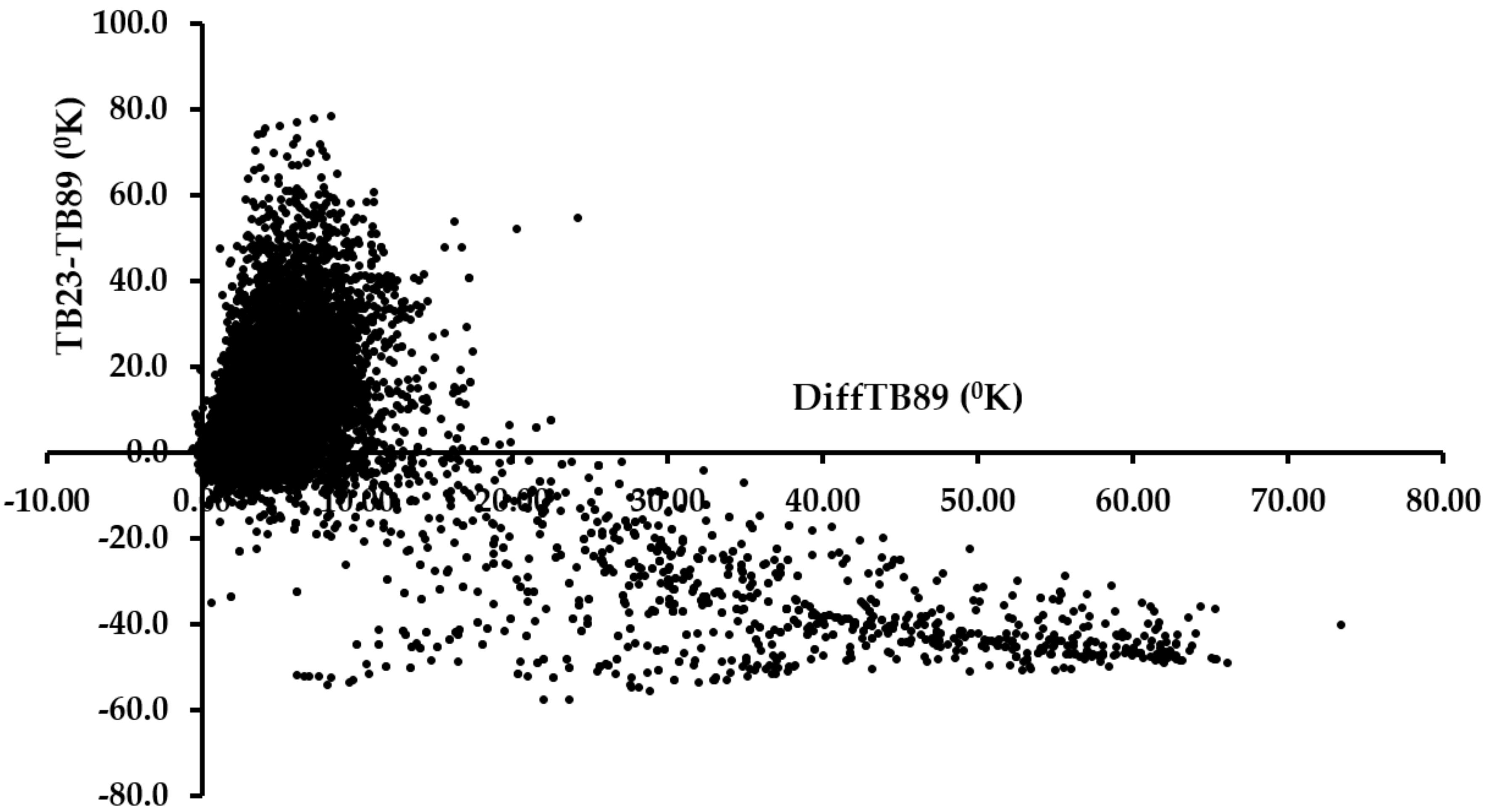
Inspection of the brightness temperature variations in the matched dataset revealed that GMI spectral signature of cases close to the coast had a distinct pattern characteristic of water surfaces: a large brightness temperature difference between vertical and horizontal polarization at the window channels and an increasing brightness temperature with increasing frequency. Figure 1 displays the scatter plot between the difference in the brightness temperature at 23 GHz and 89 GHz (vertical polarization, denoted as “TB23-TB89”) and the difference in vertical and horizontal brightness temperature at 89 GHz (denoted as DiffTB89). Negative values for the spectral gradient TB23-TB89 are associated with large positive values in DiffTB89. The map of diffTB89 over the continental US (not shown) confirmed that the largest values occur mostly over coastal areas. The same pattern holds for the polarization difference at 166 GHz. Most of the coastal matchup cases were filtered out by empirically using simple threshold values: a minimum of −20.0 for TB23-TB29 and a maximum of 20.0 for diffTB89.
Table 1 presents the partial correlations over land among brightness temperatures at 89 GHz and above and the measured hourly surface snowfall accumulation (in liquid water equivalent, denoted as “SFR”) for the snowfall sample. Partial correlations were computed controlling for surface temperature and humidity. Note the negative correlations between SFR and the brightness temperature (TB) at GMI water vapor absorption channels (TB166, TB183.31 ± 7 GHz or TB176, and TB183.31 ± 3 GHz or TB180), which are statistically significant (p-value < 0.01), suggesting the presence of a scattering signal to snowfall sized ice particles. Interestingly, the vertical and horizontal polarization brightness temperature difference at 166 GHz (denoted as “diffTB166”) has the highest correlation with SFR. Similarly, diff89 has higher correlation (statistically significant, p-value < 0.01) with SFR than the single channel brightness temperatures at 89 GHz, but lower than that of diffTB166.
The response of diffTB166 and diffTB89 to snowfall occurrence was examined by comparing their distributions between the snowfall and no-snowfall samples. Figure 2 displays the boxplot for diffTB166 and diffTB89: minimum, 25th percentile, median, 75th percentile, and the maximum. The mean value is also shown. Snowfall is associated with a larger sample mean and median for diffTB166 than no-snowfall, as the boxplots show. On the other hand, the mean and median for diffTB89 are close.
4.2. Logistic Regression Modeling
Table 2 through Table 7 present logistic regression modelling results obtained using IBM’s SPSS software with diffTB89 and diffTB166 as predictors (Table 2 and Table 3); single channel TB at 89 GHz and 166 GHz, horizontal and vertical polarization, as predictors (Table 4 and Table 5); and the final selected model with the statistically significant channel TBs (p-value < 0.01) as predictors (Table 6 and Table 7). For the final model, all the single channel TBs at 89 GHz and above and diffTB89 and diffTB166 were considered. For all the models considered, performance statistics reported was computed based on a threshold probability of 0.5, established as the value which yielded maximum overall classification rate.
Modelling results for diffTB89 and diffTB166 indicate statistical significance for each (Table 2, p-value < 0.01), and an overall classification rate of 69.0%, with the largest contribution (at 66.5%) coming from diffTB166 (Table 3).
Logistic regression of the four single channels as predictors (at 89 and 166 GHz, horizontal and vertical polarizations) indicate statistical significance for each channel (Table 4 and Table 5). Interestingly, the horizontal polarization at 166 GHz is the most important contributor to overall classification rate (at 61.5% out of 68.5%, Table 5). Also, the overall classification rate for the single channel model is slightly smaller than for the model with polarization differences as predictors.
Stepwise logistic regression was applied to all single channels and the polarization differences at 89 GHz and 166 GHz (Table 6 and Table 7). An overall classification rate of about 73% was achieved by including the 183.31 ± 3 GHz and 183.31 ± 7 GHz vertical polarization channels. Note in Table 7 the improved performance by adding DiffTB166 (step 2) and DiffTB89 (step 3) to TB80V, and the removal of TB89 at vertical and horizontal polarization and TB166 at vertical polarization from the final model (due to a p-value higher than 0.05).
Table 8 presents the performance statistics of the final model: POD, FAR, Overall Classification and HSS. Overall accuracy and HSS are at 73% (with a threshold classification probability of 0.5) and 0.48, respectively.
4.3. Retrieval Examples and Qualitative Assessment
The snowfall detection algorithm (Table 6) was applied to GMI to compute the probability of snowfall. To implement the algorithm, surface relative humidity information was obtained from the NOAA’s Global Forecast System (GFS) and used as weather filter (as explained above, scenes with humidity below 60% were classified as no-snowing). Surface temperature was also obtained from GFS to determine the form of precipitation (rain versus snow) and to limit retrievals down to −15.0 °C. The probability of snowfall threshold for considering a GMI pixel as snowing or no-snowing was set at 0.50.
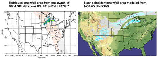
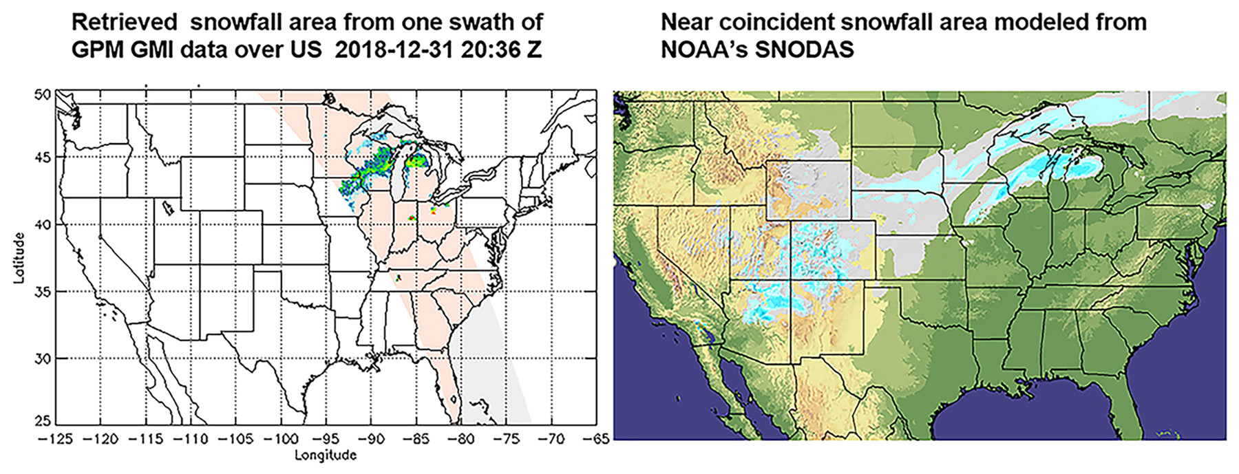
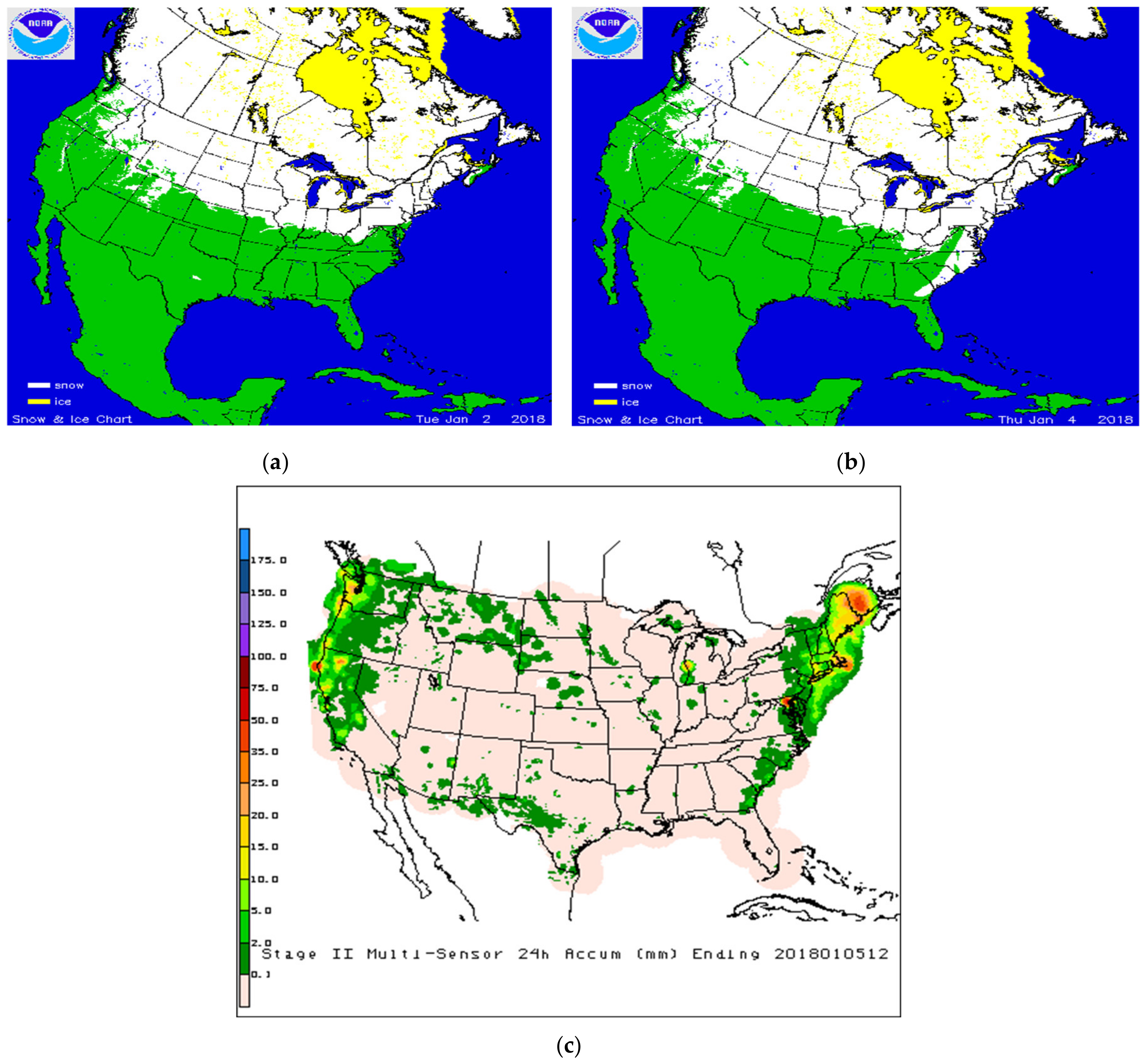
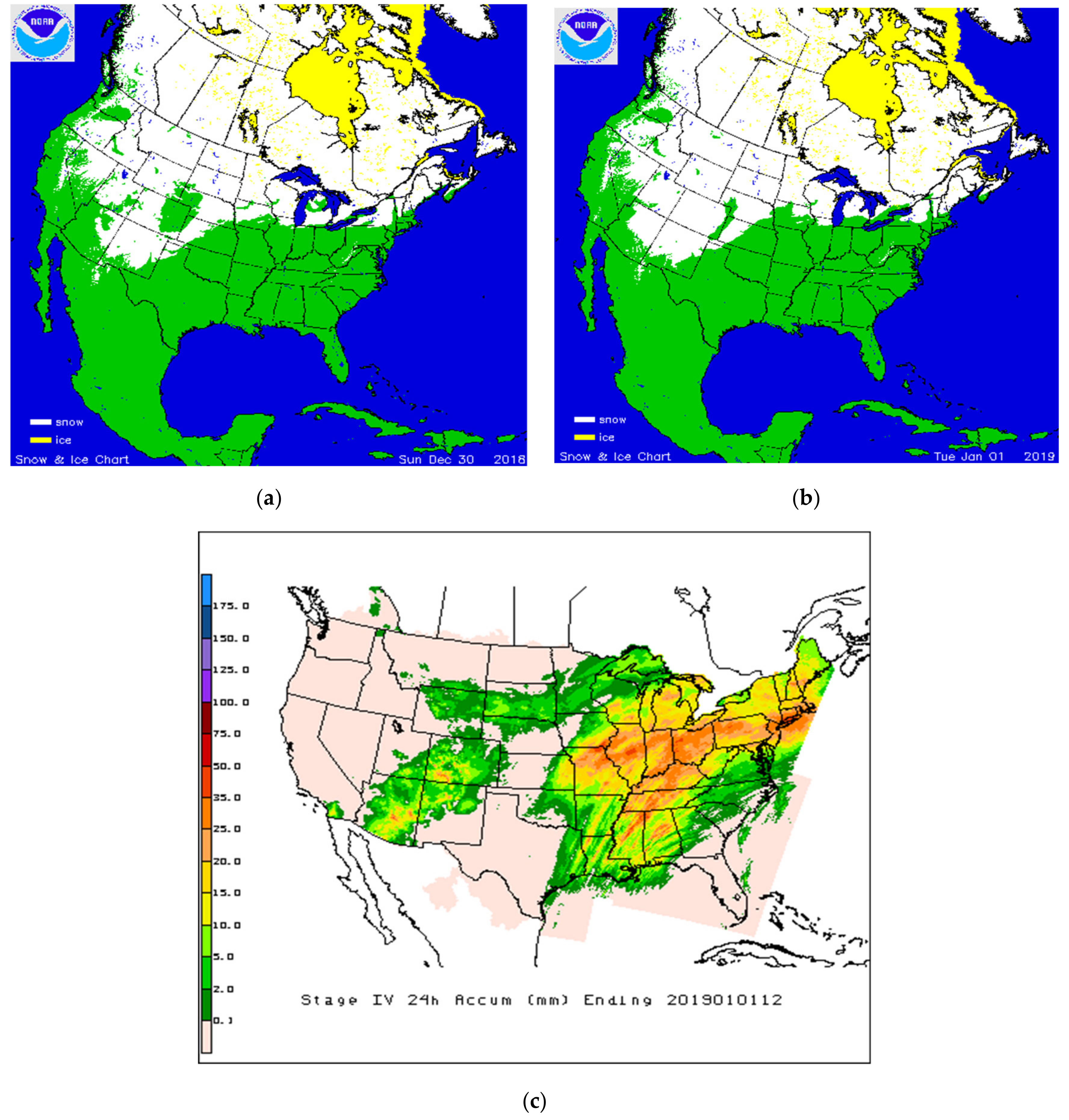
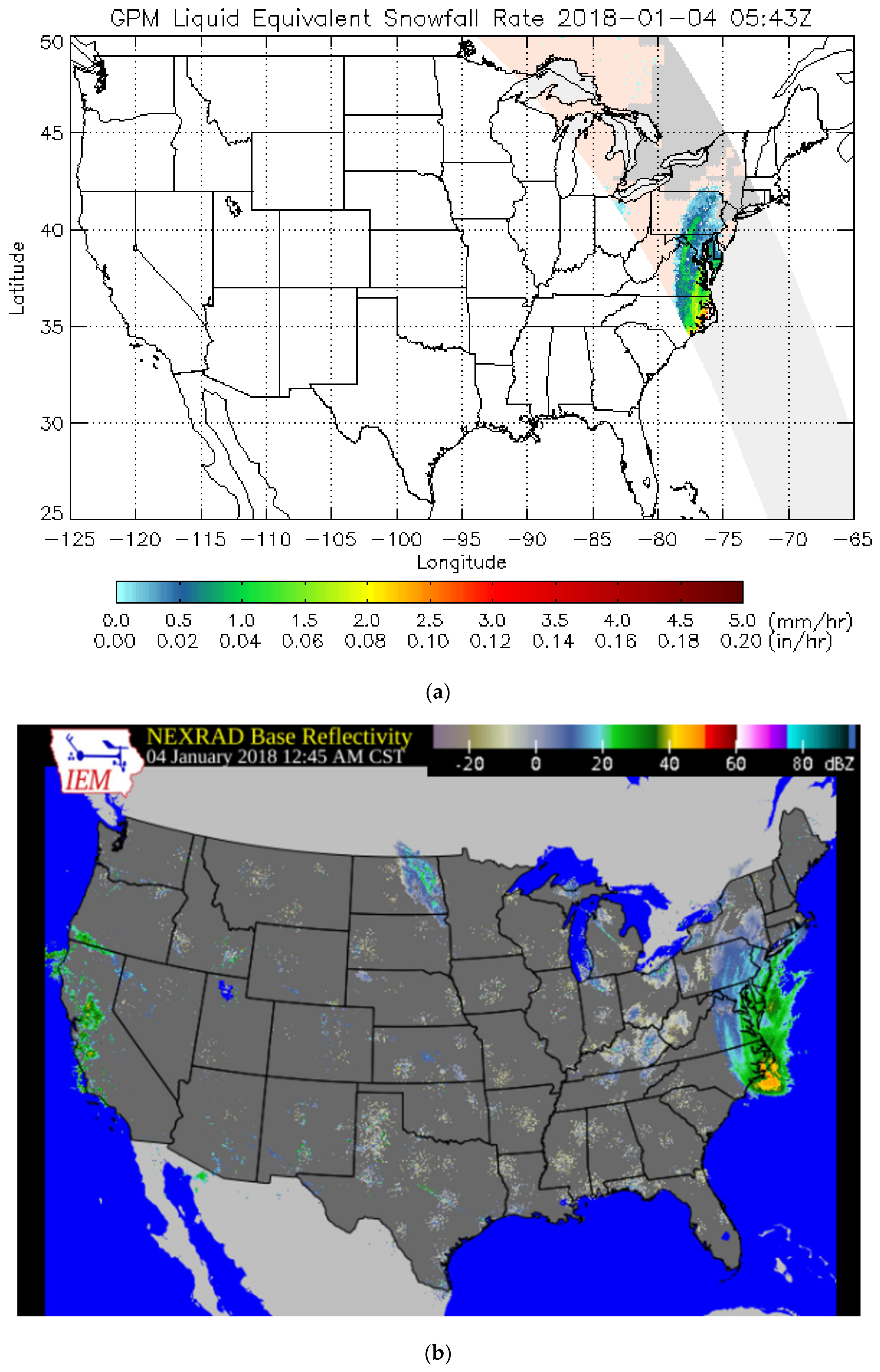
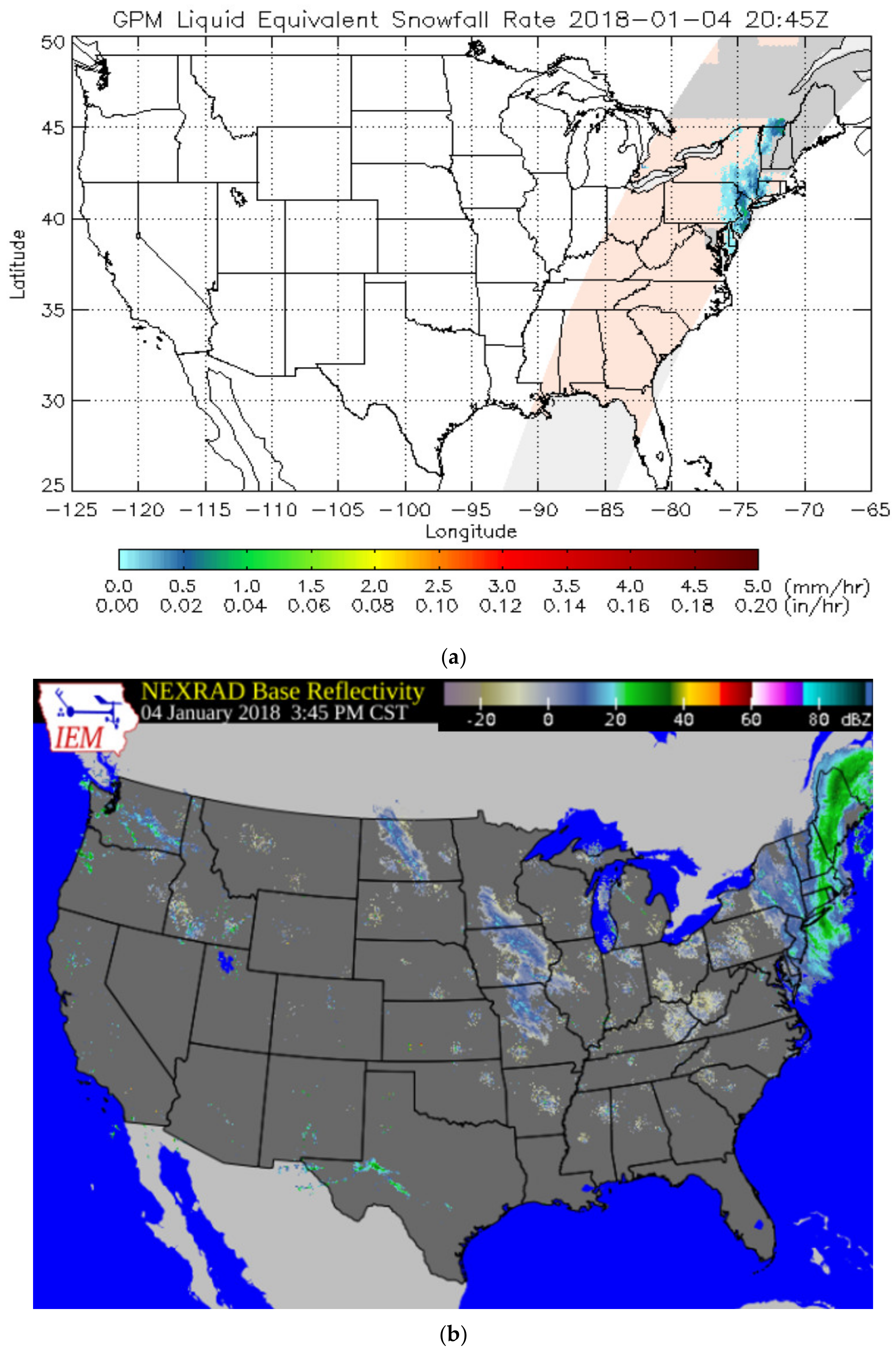
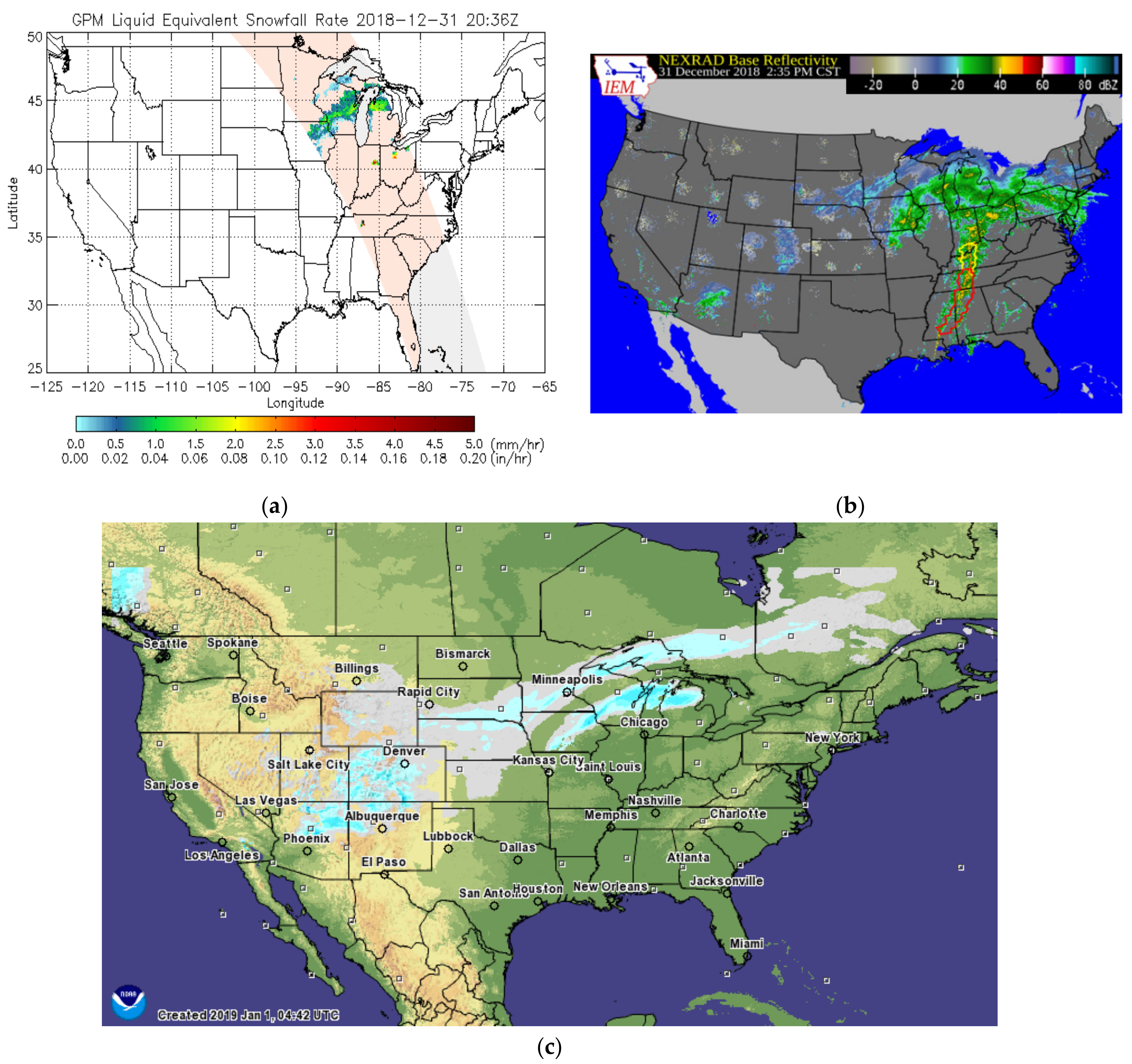
To test the robustness of the algorithm, two significant snowfall events were selected with extensive coverage over different parts of US: One event in early January 2018 that impacted eastern US and the other event in late December 2018 over central US. Figure 3 and Figure 4 show IMS snow cover maps and 24-h Stage IV precipitation accumulation on 4 January and 31 December 2018, respectively. The January 4 event hit a large portion of Eastern United States, depositing new snow on the ground in the south and new snow on snow-covered areas of the Northeast. The 31 December event deposited snow over the South-West and North-Central US and rain over Eastern US, the latter evidenced and inferred by the presence of snow-free land from IMS maps and falling precipitation (from the Stage IV product). Figure 5 and Figure 6 display swaths of GMI-based retrieval of surface precipitation rate on January 4 using NOOA’s snowfall rate algorithm ([12]) applied over GMI snowfall detected areas and near-coincident NEXRAD base reflectivity maps. Visual inspection and comparison of the maps shows detection of the distinct features of snowfall over land (coastal and ocean scenes were removed). Figure 7 shows one swath of the GMI-based retrieval on December 31 and near coincident NEXRAD base reflectivity map. Note the remarkable ability of GMI in the retrieval of two near parallel elongated snowfall areas in the upper Midwest. The massive precipitation in the South and Northeast that is shown by NEXRAD (but not shown on GMI maps) is rainfall, as evidenced by the forecast frozen hourly precipitation from SNODAS. These results demonstrate the skill of GMI high frequency measurements, with polarization difference at 89 and 166 GHz among predictors, for robust snowfall detection.
5. Discussion
This study fills an existing research gap in the exploration of the polarization difference at 166 and 89 GHz for snowfall detection. Very few studies have focused on the sensitivity of these indices to snowfall and to our knowledge none has tested the utility of these indices as independent predictors in snowfall detection algorithms.
Results of this study suggest that the polarization differences at 166 GHz and 89 GHz contain unique and useful information for the retrieval of snowfall that cannot be extracted by the single channels at these frequencies. This finding is supported by the statistical analysis of the training dataset extending over a two-year period, logistic regression modelling investigation, and the robust retrievals of two major snowfall events over continental US.
The positive correlation between the polarization difference at 166 GHz and station measured SFR suggests that this index is sensitive to the intensity of snowfall, and this result is consistent with the findings in [14,17]. As reported earlier, very light snowfall represented a large fraction of the collected snowfall sample. Note that in [17], the polarization difference at 150 GHz was found to respond to light to moderate snowfall, whereas in [14], the 166 GHz polarization difference was sensitive to moderate and heavy snowfall events.
The fact that the 166 GHz polarization difference had the highest correlation of all the GMI measurements is remarkable and suggests that the horizontally oriented ice particle structure of snowfall is a common occurrence as concluded in [16]. Sensitivity to snowfall intensity is decreased at 89 GHz, as evidenced by a smaller but statistically significant correlation value and by the fact that the distribution of the 89 GHz polarization difference index for the snowfall sample is close to that of the no-snowfall sample. In contrast, the distribution of 166 GHz polarization difference index for the snowfall sample is significantly different to that of the no-snowfall sample. Not only the snowfall sample mean is larger than the no-snowfall sample (4.2 K versus 2.2 K) but also the variance is larger: the standard deviation is 3.6 K for the snowfall sample and 2.2 K for the no-snowfall sample. For the polarization difference index at 89 GHz, these statistics are very close: the mean value is equal to 4.5 K for the snowfall sample and 4.6 K for the no-snowfall sample, and the standard deviation is equal to 2.7 K for the snowfall and no-snowfall sample.
The logistic regression modelling investigation showed that these GMI indices have substantial prognostic capability for snowfall detection, a finding that has been overlooked, perhaps due to the treatment of the problem of snowfall detection as a machine learning exercise. Based on the physical understanding of the problem gained from prior studies [14,16,17], we hypothesized that these polarization indices are sensitive to snowfall, tested them as independent predictors, and found that results are remarkable. They show statistical significance and an impressive overall snowfall classification rate of 69.0%, with the largest contribution (at 66.5%) coming from the polarization difference at 166 GHz. Logistic regression of the four single channels as predictors (at 89 and 166 GHz, horizontal and vertical polarizations) showed that the horizontal 166 GHz channel was the most important predictor (at 61.5% out of 68.5%).
Stepwise logistic regression applied to all single channels at 89 GHz and above and the polarization difference at 89 and 166 GHz achieved an overall classification rate of 73%. The increased performance was mainly due to the inclusion of the 183.31 ± 3 GHz and 183.31 ± 7 GHz vertical polarization channels. Of notable interest is the improved performance of the final model when the polarization difference at 166 GHz and 89 GHz was added to the water vapor absorption channel at 180 GHz, and that the single channel brightness temperatures at 89 GHz and the vertical polarization brightness temperature at 166 GHz were removed from the final model (due to being statistically non-significant at a p-value = 0.05), but not the polarization differences.
6. Conclusions
In this study, we tested the utility of the GMI high frequency measurements at 89 GHz and above for snowfall detection, with a focus on the polarization difference at 89 and 166 GHz. Statistical analysis of the GMI data matched to ground truth station observations over a two-year period and qualitative assessment of the final logistic regression algorithm showed the following:
The 166 GHz polarization difference was the most sensitive GMI high frequency measurement to station-measured snowfall intensity. Sensitivity to snowfall intensity is decreased at 89 GHz polarization difference but is non-the-less statistically significant.
The polarization difference at 166 GHz has substantial predictive ability, giving an overall classification rate of 66% as a single predictor to the probability of snowfall, out of a maximum of 73% when using the final selected logistic regression model.
Both these polarization indices are retained in the final selected model while single channel measurements at 89 GHz and the vertical polarization at 166 GHz are removed (as non-significant), a testament to the unique information content of these indices and their utility in snowfall detection algorithms.
The final logistic regression algorithm showed clear skill in capturing two significant snowfall events in a semi operational environment at NOAA/NESDIS. Future work is needed to assess the performance of the algorithm in a wide variety of weather conditions and snowfall events before the algorithm can be deemed generally applicable and operationally acceptable.
Author Contributions
C.K. wrote the paper with contributions from all the co-authors. H.M., J.D., and R.F. contributed to conceptualization, analysis, and review of the paper. All authors have read and agreed to the published version of the manuscript.
Funding
This research was funded by National Oceanic and Atmospheric Administration (NOAA), grant number NA18NWS4680053.
Acknowledgments
We thank the anonymous reviewers for their valuable comments and suggestions. The views, opinions, and findings contained in this report are those of the authors and should not be construed as an official National Oceanic and Atmospheric Administration or U.S. Government position, policy, or decision.
Conflicts of Interest
The authors declare no conflict of interest.
References
- Liu, G.; Curry, J.A. Precipitation Characteristics in Greenland-Iceland-Norwegian Seas Determined by Using Satellite Microwave Data. J. Geophys. Res. 1997, 102, 13987–13997. [Google Scholar] [CrossRef]
- Staelin, D.H.; Chen, F.W. Precipitation Observations Near 54 and 183 GHz using the NOAA-15 Satellite. IEEE Trans. Geosci. Remote Sens. 2000, 38, 2322–2332. [Google Scholar] [CrossRef] [Green Version]
- Chen, F.W.; Staelin, D.H. AIRS/AMSU/HSB precipitation estimates. IEEE Trans. Geosci. Remote Sens. 2003, 41, 410–417. [Google Scholar] [CrossRef] [Green Version]
- Kongoli, C.; Pellegrino, P.; Ferraro, R.R.; Grody, N.C.; Meng, H. A New Snowfall Detection Algorithm Over Land Using Measurements from the Advanced Microwave Sounding Unit (AMSU). Geophys. Res. Lett. 2003, 30, 1756–1759. [Google Scholar] [CrossRef]
- Skofronick-Jackson, G.; Kim, M.-J.; Weinman, J.; Chang, D.-E. A Physical Model to Determine Snowfall Over Land by Microwave Radiometry. IEEE Trans. Geosci. Remote Sens. 2004, 42, 1047–1058. [Google Scholar] [CrossRef] [Green Version]
- Noh, Y.-J.; Liu, G.; Seo, E.-K.; Wang, J.; Aonashi, K. Development of a Snowfall Retrieval Algorithm at High Microwave Frequencies. J. Geophys. Res. 2006, 111, D22216. [Google Scholar] [CrossRef]
- Liu, G.; Seo, E. Detecting Snowfall Over Land by Satellite High-Frequency Microwave Observations: The Lack of Scattering Signature and a Statistical Approach. J. Geophys. Res. Atmos. 2013, 118, 1376–1387. [Google Scholar] [CrossRef]
- Ferraro, R.R.; Weng, F.; Grody, N.; Zhao, L.; Meng, H.; Kongoli, C.; Pellegrino, P.; Qiu, S.; Dean, C. NOAA Operational Hydrological Products Derived from the AMSU. IEEE Trans. Geosci. Remote Sens. 2005, 43, 1036–1049. [Google Scholar] [CrossRef]
- Surussavadee, C.; Blackwell, W.J.; Entekhabi, D.; Leslie, R.V. A Global Precipitation Retrieval Algorithm for Suomi NPP ATMS. In Proceedings of the Geoscience and Remote Sensing Symposium (IGARSS), Munich, Germany, 22–27 July 2012; pp. 1924–1927. [Google Scholar]
- Kongoli, C.; Meng, H.; Meng, J.; Ferraro, R. A Snowfall Detection Algorithm Over Land Utilizing High-Frequency Passive Microwave Measurements—Application to ATMS. JGR-Atmos. 2015, 120, 1918–1932. [Google Scholar] [CrossRef]
- Kongoli, C.; Meng, H.; Dong, J.; Ferraro, R. A Hybrid Snowfall Detection Method from Satellite Passive Microwave Measurements and Global Weather Forecast Models. Q. J. R. Meteorol. Soc. 2018, 144, 120–132. [Google Scholar] [CrossRef] [Green Version]
- Meng, H.; Dong, J.; Ferraro, R.; Yan, B.; Zhao, L.; Kongoli, C.; Wang, N.-Y.; Zavodsky, B. A 1DVAR-Based Snowfall Rate Retrieval Algorithm for Passive Microwave Radiometers. J. Geophys. Res. Atmos. 2017, 122, 6520–6540. [Google Scholar] [CrossRef]
- You, Y.; Wang, N.-Y.; Ferraro, R.; Rudolski, S. Quantifying the Snowfall Detection Performance of the GPM Microwave Imager Channels over Land. J. Hydrometeor. 2017, 18, 729–751. [Google Scholar] [CrossRef]
- Panegrossi, G.; Rysman, J.-F.; Daniele, C.; Marra, A.; Sano, P.; Kulie, M. CloudSat-Based Assessment of GPM Microwave Imager Snowfall Observation Capabilities. Remote Sens. 2017, 9, 1263. [Google Scholar] [CrossRef] [Green Version]
- Zeng, X.; Skofronick-Jackson, G.; Tian, L.; Emory, A.E.; Olson, W.S.; Kroodsma, R.A. Analysis of the Global Microwave Polarization Data of Clouds. J. Clim. 2019, 32, 3–13. [Google Scholar] [CrossRef] [Green Version]
- Ebtehaj, A.M.; Kummerow, C.D. Microwave Retrievals of Terrestrial Precipitation Over Snow-Covered Surfaces: A Lesson from the GPM Satellite. Geophys. Res. Lett. 2017, 44, 6154–6162. [Google Scholar] [CrossRef]
- Xie, X.; Crewell, S.; Löhnert, U.; Simmer, C.; Miao, J. Polarization Signatures and Brightness Temperatures Caused by Horizontally Oriented Snow Particles at Microwave Bands: Effects of Atmospheric Absorption. J. Geophys. Res. Atmos. 2015, 120, 6145–6160. [Google Scholar] [CrossRef]
- Iowa Environmental Mesonet. Available online: https://mesonet.agron.iastate.edu/docs/nexrad_mosaic/ (accessed on 27 September 2005).
- Helfrich, S.R.; McNamara, D.; Ramsay, B.H.; Baldwin, T.; Kasheta, T. Enhancements to, and Forthcoming Developments in the Interactive Multisensor Snow and Ice Mapping System (IMS). Hydrol. Proc. 2007, 21, 1576–1586. [Google Scholar] [CrossRef]
- Carroll, T.; Cline, D.; Fall, G.; Nilsson, A.; Li, L.; Rost, A. NOHRSC Operations and the Simulation of Snow Cover Properties for the Conterminous, U.S. In Proceedings of the 69th Annual Meeting of the Western Snow Conference, Sun Valley, ID, USA, 16–19 April 2001; pp. 1–14. [Google Scholar]
- Lin, Y.; Mitchell, K.E. The NCEP Stage II/IV Hourly Precipitation Analyses: Development and Applications, preprints. In Proceedings of the 19th Conf. on Hydrology, American Meteorological Society, San Diego, CA, USA, 9–13 January 2005. [Google Scholar]
- Wilks, D.S. Statistical Methods in the Atmospheric Sciences; Elsevier: Amsterdam, The Netherlands, 2011. [Google Scholar]
Figure 1.
Scatterplot between the difference in Global Precipitation Measurement (GPM) Microwave Imager (GMI) brightness temperature at 23 GHz and 89 GHz (TB23-TB89) and the vertical and horizontal polarization brightness temperature difference at 89 GHz (DiffTB89).
Figure 1.
Scatterplot between the difference in Global Precipitation Measurement (GPM) Microwave Imager (GMI) brightness temperature at 23 GHz and 89 GHz (TB23-TB89) and the vertical and horizontal polarization brightness temperature difference at 89 GHz (DiffTB89).

Figure 2.
Boxplot of summary statistics—minimum, 25th percentile, median, mean, 75th percentile and maximum—for GMI vertical and horizontal polarization brightness temperature difference at (a) 166 GHz (DiffTB166) and (b) 89 GHz (DiffTBTB89) for the snowfall and no-snowfall sample. The green line indicates the mean value and the red line indicates the median value.

Figure 3.
IMS snow maps on (a) 2 January and (b) 4 January 2018, respectively, and (c) NCEP Stage IV Multi-Sensor 24 h precipitation accumulation ending 5 January 2018 12 Zulu time.
Figure 3.
IMS snow maps on (a) 2 January and (b) 4 January 2018, respectively, and (c) NCEP Stage IV Multi-Sensor 24 h precipitation accumulation ending 5 January 2018 12 Zulu time.

Figure 4.
IMS snow maps on (a) 30 December 2018 and (b) 1 January 2019, respectively, and (c) NCEP Stage IV Multi-Sensor 24 h precipitation accumulation ending 1 January 2019 12 Zulu time.
Figure 4.
IMS snow maps on (a) 30 December 2018 and (b) 1 January 2019, respectively, and (c) NCEP Stage IV Multi-Sensor 24 h precipitation accumulation ending 1 January 2019 12 Zulu time.

Figure 5.
(a) Retrieved GMI-based Liquid Water Snowfall Rate in mm hr−1 on 4 January 2018 5:43 Zulu time and (b) near coincident NEXRAD base reflectivity in dbZ.
Figure 5.
(a) Retrieved GMI-based Liquid Water Snowfall Rate in mm hr−1 on 4 January 2018 5:43 Zulu time and (b) near coincident NEXRAD base reflectivity in dbZ.

Figure 6.
(a) Retrieved GMI-based Liquid Water Snowfall Rate in mm hr−1 (top) on 4 January 2018 20:45 Zulu time and (b) neat coincident NEXRAD base reflectivity in dbZ.
Figure 6.
(a) Retrieved GMI-based Liquid Water Snowfall Rate in mm hr−1 (top) on 4 January 2018 20:45 Zulu time and (b) neat coincident NEXRAD base reflectivity in dbZ.

Figure 7.
(a) Retrieved GMI-based Liquid Water Snowfall Rate in mm hr−1 on 31 December 2018 20:36 Zulu time, (b) near coincident NEXRAD base reflectivity in dbZ, and (c) near coincident hourly snowfall accumulation from NOAA SNODAS.
Figure 7.
(a) Retrieved GMI-based Liquid Water Snowfall Rate in mm hr−1 on 31 December 2018 20:36 Zulu time, (b) near coincident NEXRAD base reflectivity in dbZ, and (c) near coincident hourly snowfall accumulation from NOAA SNODAS.


Table 1.
Partial correlation coefficients over land among GMI brightness temperature measurements and station measured snowfall rate (SFR). For the variable names, “TB” denotes the brightness temperature, “H” and “V” denote vertical and horizontal polarizations, and the numbers denote the channel center frequency. “diff” refers to the vertical and horizontal brightness temperature difference at a specific frequency. Control variables are the measured surface temperature and relative humidity.
| diffTB166 | TB166V | TB166H | TB180V * | TB176V ** | SFR | TB89V | TB89H | difTB89 | |
|---|---|---|---|---|---|---|---|---|---|
| diffTB166 | 1.00 | −0.69 | −0.79 | −0.40 | −0.69 | 0.24 | −0.36 | −0.47 | 0.59 |
| TB166V | −0.69 | 1.00 | 0.99 | 0.43 | 0.84 | −0.18 | 0.75 | 0.77 | −0.36 |
| TB166H | −0.79 | 0.99 | 1.00 | 0.45 | 0.86 | −0.21 | 0.71 | 0.75 | −0.43 |
| TB180V* | −0.40 | 0.43 | 0.45 | 1.00 | 0.73 | −0.17 | 0.20 | 0.20 | −0.08 |
| TB176V** | −0.69 | 0.84 | 0.86 | 0.73 | 1.00 | −0.22 | 0.45 | 0.46 | −0.24 |
| SFR | 0.24 | −0.18 | −0.21 | −0.17 | −0.22 | 1.00 | −0.06 | −0.07 | 0.07 |
| TB89V | −0.36 | 0.75 | 0.71 | 0.20 | 0.45 | −0.06 | 1.00 | 0.97 | −0.27 |
| TB89H | −0.47 | 0.77 | 0.75 | 0.20 | 0.46 | −0.07 | 0.97 | 1.00 | −0.49 |
| difTB89 | 0.59 | −0.36 | −0.43 | −0.08 | −0.24 | 0.07 | −0.27 | −0.49 | 1.00 |
* TB180V denotes brightness temperature at 183.31 ± 3 GHz with vertical polarization. ** TB176V denotes brightness temperature at 183.31 ± 7 GHz with vertical polarization.
Table 2.
Logistic regression model coefficients and statistics for the vertical and horizontal polarization brightness temperature difference at GMI 166 GHz (DiffTB166) and 89 GHz (DiffTB89) as predictors. “B” indicates the partial regression coefficient, “SE” indicates the standard error and “Wald” indicates the observed Wald test statistic.
| Predictors | B | SE | Wald | p-Value |
|---|---|---|---|---|
| DiffTB166 | 0.393 | 0.012 | 1145.124 | <0.01 |
| DiffTB89 | −0.264 | 0.011 | 536.571 | <0.01 |
| Intercept | −0.406 | 0.042 | 91.708 | <0.01 |
Table 3.
Forward stepwise logistic regression model performances for diffTB166 (step 1) and diddTB166 and diffTB89 (step 2) as predictors. Each step shows results from the logistic regression model with a new additional predictor variable. “df” indicates the degrees of freedom, “Chi-square” represents the observed Chi-square test statistic value, and “Correct Class” represents the correct overall classification rate.
| Step | Improvement | Model | Correct Class % | Variable | ||||
|---|---|---|---|---|---|---|---|---|
| Chi-Square | df | p-Value. | Chi-Square | df | p-Value. | |||
| 1 | 912.81 | 1 | <0.01 | 912.81 | 1 | <0.01 | 66.50% | IN: diffTB166 |
| 2 | 636.473 | 1 | <0.01 | 1549.283 | 2 | <0.01 | 68.90% | IN: difTB89 |
Table 4.
Logistic regression model coefficients and statistics for single channel brightness temperature measurements, vertical and horizontal polarization, at 166 GHz (TB166 V and TB166H) and 89 GHz (TB89V and TB89H) as predictors. “B” indicates the partial regression coefficients, “SE” indicates the standard error, and “Wald” indicates the observed Wald test statistic.
| Predictors | B | SE | Wald | p-Value |
|---|---|---|---|---|
| TB166V | 0.331 | 0.017 | 398.942 | 0.00 |
| TB166H | −0.357 | 0.014 | 644.903 | 0.00 |
| TB89V | −0.23 | 0.012 | 347.841 | 0.00 |
| TB89H | 0.252 | 0.012 | 468.638 | 0.00 |
| Intercept | 0.887 | 0.618 | 2.059 | 0.00 |
Table 5.
Forward stepwise logistic regression model significance test results and performances for single channel brightness temperature measurements, vertical and horizontal polarization, at 166 GHz (TB166 V and TB166H) and 89 GHz (TB89V and TB89H) as predictors. Each step shows results from the logistic regression model with a new additional predictor variable. “df” indicates the degrees of freedom, “Chi-square” represents the observed Chi-square test statistic value, and “Correct Class” represents the correct overall classification rate.
| Step | Improvement | Model | Correct Class % | Variable | ||||
|---|---|---|---|---|---|---|---|---|
| Chi-Square | df | p-Value | Chi-Square | df | p-Value | |||
| 1 | 492.387 | 1 | <0.01 | 492.387 | 1 | <0.01 | 61.50% | IN: TB166H |
| 2 | 585.218 | 1 | <0.01 | 1077.605 | 2 | <0.01 | 64.10% | IN: TB89H |
| 3 | 139.115 | 1 | <0.01 | 1216.721 | 3 | <0.01 | 66.70% | IN: TB166V |
| 4 | 387.087 | 1 | <0.01 | 1603.807 | 4 | <0.01 | 68.50% | IN: TB89V |
Table 6.
Final logistic regression model results after the stepwise selection was applied to all high frequency channel TBs at 89 GHz and above and the vertical and horizontal brightness temperature polarization difference at 89 (diffTB89) and 166 (diffTB166) GHz. “B” indicates the partial regression coefficients, “SE” indicates the standard error and “Wald” indicates the observed Wald test statistic.
| Predictors | B | SE | Wald | p-Value |
|---|---|---|---|---|
| TB180V | −0.15 | 0.01 | 242.333 | <0.01 |
| TB176V | −0.105 | 0.012 | 72.709 | <0.01 |
| DiffTB166 | 0.308 | 0.015 | 394.763 | <0.01 |
| TB166H | 0.057 | 0.005 | 128.317 | <0.01 |
| diffTB89 | −0.144 | 0.012 | 134.749 | <0.01 |
| Intercept | 49.56 | 1.858 | 711.76 | <0.01 |
Table 7.
Forward stepwise logistic regression model performances for the final model. Each step shows results from the logistic regression model with a new additional predictor variable.
Table 7.
Forward stepwise logistic regression model performances for the final model. Each step shows results from the logistic regression model with a new additional predictor variable.
| Step | Improvement | Model | Correct Class % | Variable | ||||
|---|---|---|---|---|---|---|---|---|
| Chi-Square | df | Sig. | Chi-Square | df | Sig. | |||
| 1 | 2038.087 | 1 | 0 | 2038.087 | 1 | 0 | 69.40% | IN: TB180V |
| 2 | 138.929 | 1 | 0 | 2177.016 | 2 | 0 | 70.50% | IN: diffTB166 |
| 3 | 294.03 | 1 | 0 | 2471.046 | 3 | 0 | 71.80% | IN: difTB89 |
| 4 | 92.522 | 1 | 0 | 2563.568 | 4 | 0 | 72.00% | IN: TB89H |
| 5 | 11.814 | 1 | 0.001 | 2575.381 | 5 | 0 | 72.00% | IN: TB176V |
| 6 | 39.319 | 1 | 0 | 2614.701 | 6 | 0 | 72.60% | IN: TB166H |
| 7 | −0.385 | 1 | 0.535 | 2614.315 | 5 | 0 | 72.60% | OUT: TB89H |
“df” indicates the degrees of freedom. “Chi-square” represents the observed Chi-square test statistic value, and “Correct Class” represents the correct overall classification rate.
Table 8.
Performance statistics of the final logistic regression model. POD indicates the probability of snowfall detection, FAR indicates the probability of false alarm, and HSS indicates the Heidke Skill Score.
Table 8.
Performance statistics of the final logistic regression model. POD indicates the probability of snowfall detection, FAR indicates the probability of false alarm, and HSS indicates the Heidke Skill Score.
| POD | FAR | Overall | HSS |
|---|---|---|---|
| 57.3 | 13.0 | 72.6 | 0.48 |
Publisher’s Note: MDPI stays neutral with regard to jurisdictional claims in published maps and institutional affiliations. |
© 2020 by the authors. Licensee MDPI, Basel, Switzerland. This article is an open access article distributed under the terms and conditions of the Creative Commons Attribution (CC BY) license (http://creativecommons.org/licenses/by/4.0/).
Share and Cite
MDPI and ACS Style
Kongoli, C.; Meng, H.; Dong, J.; Ferraro, R. Ground-based Assessment of Snowfall Detection over Land Using Polarimetric High Frequency Microwave Measurements. Remote Sens. 2020, 12, 3441. https://0-doi-org.brum.beds.ac.uk/10.3390/rs12203441
AMA Style
Kongoli C, Meng H, Dong J, Ferraro R. Ground-based Assessment of Snowfall Detection over Land Using Polarimetric High Frequency Microwave Measurements. Remote Sensing. 2020; 12(20):3441. https://0-doi-org.brum.beds.ac.uk/10.3390/rs12203441
Chicago/Turabian StyleKongoli, Cezar, Huan Meng, Jun Dong, and Ralph Ferraro. 2020. "Ground-based Assessment of Snowfall Detection over Land Using Polarimetric High Frequency Microwave Measurements" Remote Sensing 12, no. 20: 3441. https://0-doi-org.brum.beds.ac.uk/10.3390/rs12203441
Note that from the first issue of 2016, this journal uses article numbers instead of page numbers. See further details here.