Towards DCS in the UV Spectral Range for Remote Sensing of Atmospheric Trace Gases


Institut Lumière Matière, Université Claude Bernard Lyon 1, University of Lyon, CNRS, F-69622 Villeurbanne, France
*
Author to whom correspondence should be addressed.
Remote Sens. 2020, 12(20), 3444; https://0-doi-org.brum.beds.ac.uk/10.3390/rs12203444
Submission received: 11 September 2020
/
Revised: 13 October 2020
/
Accepted: 14 October 2020
/
Published: 20 October 2020
(This article belongs to the Special Issue Advances in Atmospheric Remote Sensing with Lidar)
Abstract
:The development of increasingly sensitive and robust instruments and new methodologies are essential to improve our understanding of the Earth’s climate and air pollution. In this context, Dual-Comb spectroscopy (DCS) has been successfully demonstrated as a remote laser-based instrument to probe infrared absorbing species such as greenhouse gases. We present here a study of the sensitivity of Dual-Comb spectroscopy to remotely monitor atmospheric gases focusing on molecules that absorb in the ultraviolet domain, where the most reactive molecules of the atmosphere (OH, HONO, BrO...) have their highest absorption cross-sections. We assess the achievable signal-to-noise ratio (SNR) and the corresponding minimum absorption sensitivity of DCS in the ultraviolet range. We propose a potential light source for remote sensing UV-DCS and discuss the degree of immunity of UV-DCS to atmospheric turbulences. We show that the characteristics of the currently available UV sources are compatible with the unambiguous identification of UV absorbing gases by UV-DCS.
| Contents | ||
| 1 | Introduction | 2 |
| 2 | Dual-Comb Spectroscopy | 3 |
| 2.1 Principle............................................................................................................................................................................ | 3 | |
| 2.2 UV-DCS Spectrometer Signal Fluctuations.................................................................................................................... | 5 | |
| 3 | UV-DCS Laser Sources | 6 |
| 4 | UV Light Propagation into the Atmosphere | 8 |
| 4.1 Atmosphere-Induced Amplitude Noise.......................................................................................................................... | 8 | |
| 4.2 Atmosphere-Induced Phase Noise................................................................................................................................... | 8 | |
| 5 | Results: Simulated UV-DCS Sensitivity | 9 |
| 5.1 Quality Factor and Minimum Absorption Sensitivity................................................................................................... | 9 | |
| 5.2 Case (1): 308 nm: Narrow Spectral Range and High Spectral Resolution.................................................................. | 10 | |
| 5.3 Case (2): 350 nm: Broad Spectral Range and Low Spectral Resolution....................................................................... | 11 | |
| 5.4 Results on Concentration Detection Limits.................................................................................................................... | 11 | |
| 6 | Discussion | 12 |
| 7 | Conclusions | 13 |
| A Multiplicative Noise Due to Residual Relative Optical Phase Noise | 14 | |
| References | 15 | |
1. Introduction
The impact of atmospheric pollution on environment, climate, and human health continues to escalate on a global scale [1] despite considerable progress made to develop air-quality monitoring and to provide worldwide environmental policies. Reasons for this rise are numerous and include an insufficient knowledge of the atmospheric processes involved. Greater knowledge involves a better understanding of the fundamental physical and chemical processes of the atmosphere, a better understanding of the composition of the atmosphere and the development of more sensitive monitoring devices for the minor and very reactive compounds like the hydroxyl radical OH. In this context, air pollution measurement and monitoring devices based on absorption spectroscopy contribute significantly. These measurements can be done anywhere from the ground level up to the stratosphere using ground-based platforms [2]. Using instruments on satellite-based platforms, absorption spectroscopy is also employed for large scale observations of air pollution dispersion [3,4,5]. Different experimental arrangements have been developed covering the ultraviolet (UV) out to the infrared (IR) using coherent or non-coherent light sources: Differential Optical Absorption spectroscopy (DOAS) [6], Fourier-Transform Infrared (FTIR) spectroscopy [7], Cavity-Ring Down spectroscopy (CRDS) [8,9,10], and Differential Absorption Lidar (DIAL) [11,12]. The advantage of these methodologies when they are coupled with a remote sensing technique is that atmospheric compounds can be probed in situ without air sampling. This aspect is particularly important when highly reactive molecules like OH, HONO, BrO, and O3 are to be monitored [6], likewise for atmospheric aerosols [13,14].
To improve the knowledge on air quality, several approaches can be adopted depending on species concentration. Many methodologies exist for abundant compounds, where combined analysis from low sensitivity and low accuracy devices network can be interpreted applying the neural network algorithm [15,16,17]. For trace species contributing significantly to the atmospheric chemistry and physics, instruments need accuracy, sensitivity, and sampling frequency improvements. Because the atmosphere is a complex system, instruments based on absorption spectroscopy suffer from the contribution of other compounds in the same spectral range resulting in concentration bias. This highlights the necessity of developing monitoring instruments that operate over a large spectral range with a high spectral resolution. Fourier transform spectrometers and broadband cavity enhanced spectroscopy [18,19] seem to fulfill these requirements.
This work presents the performances in terms of concentration detection limit of Dual-Comb spectroscopy in the UV range in a perspective to integrate it in a remote sensing device as the Integrated Path Lidar (IP-LIDAR) [20,21] and broadband Lidar [22,23]. DCS is a Fourier-transform type experiment that takes advantage of mode-locked femtosecond (fs) pulses. This emerging spectroscopy methodology appears highly relevant for atmosphere remote-sensing studies because of its very fast acquisition rate (>kHz) that reduces the impact of atmospheric turbulences on the retrieved spectra. DCS has been successfully applied in near-infrared (NIR) spectral ranges for atmospheric greenhouse gas monitoring (water vapor, carbon dioxide, and methane) [24,25,26]. The degree of technological maturity in this spectral region allows compact devices and simplified DCS architectures to be implemented [27,28]. The extension to the mid-infrared wavelength exploits parametric generation as difference frequency generation [29]. References [30,31] give useful reviews for an overview of the implemented sources for Dual-Comb spectroscopy. UV molecular transitions have been probed using DCS by two-photon absorption spectroscopy in the red spectral range [32]. In the present paper, we estimate the sensitivity the UV-DCS could offer to probe atmospheric trace gases (OH, BrO, NO2, OClO, HONO, CH2O, SO2) directly in the UV spectral range, where their absorption cross-sections are greatest. We estimate the sensitivity of UV-DCS for two case-studies, chosen for their relevance for open-air remote sensing of specific atmospheric molecules. Case (1) represents a high resolution experiment at 308 nm in a narrow spectral range (1 THz, 0.3 nm, 33 cm−1). This spectral range is of high interest for trace gas monitoring since it allows a possible simultaneous measurement of naphthalene (C8H10), sulphur dioxide (SO2), formaldehyde (HCHO) and hydroxide radical (OH). Secondly, we study the case of a low-resolution experiment centred at 350 nm over a wide spectral range of approximately 50 THz (20 nm, 1730 cm−1), referred as Case (2), where for example bromine oxide (BrO) and nitrous acid (HONO) present their highest absorption. The spectral range and resolution of the two case-studies are consistent with the ones reported by existing similar methodologies like UV-DOAS (a spectrometer coupled to a remote sensing optical device) and they allow an adequate evaluation of the interfering gases.
The manuscript is presented as follows. The principle of Dual-Comb spectroscopy and the source of signal fluctuations are presented in Section 2. Section 3 discusses the extension of DCS into the UV range and we conclude on a potential laser source of UV-DCS. Section 4 highlights measurement noises due to the laser beam propagation through the atmosphere. A sensitivity study of the DCS method in the UV range is presented in Section 5 for the two case-studies.
2. Dual-Comb Spectroscopy
2.1. Principle
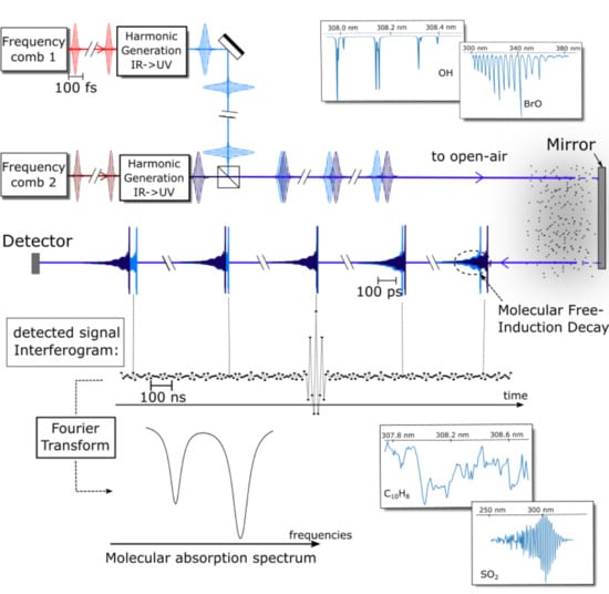
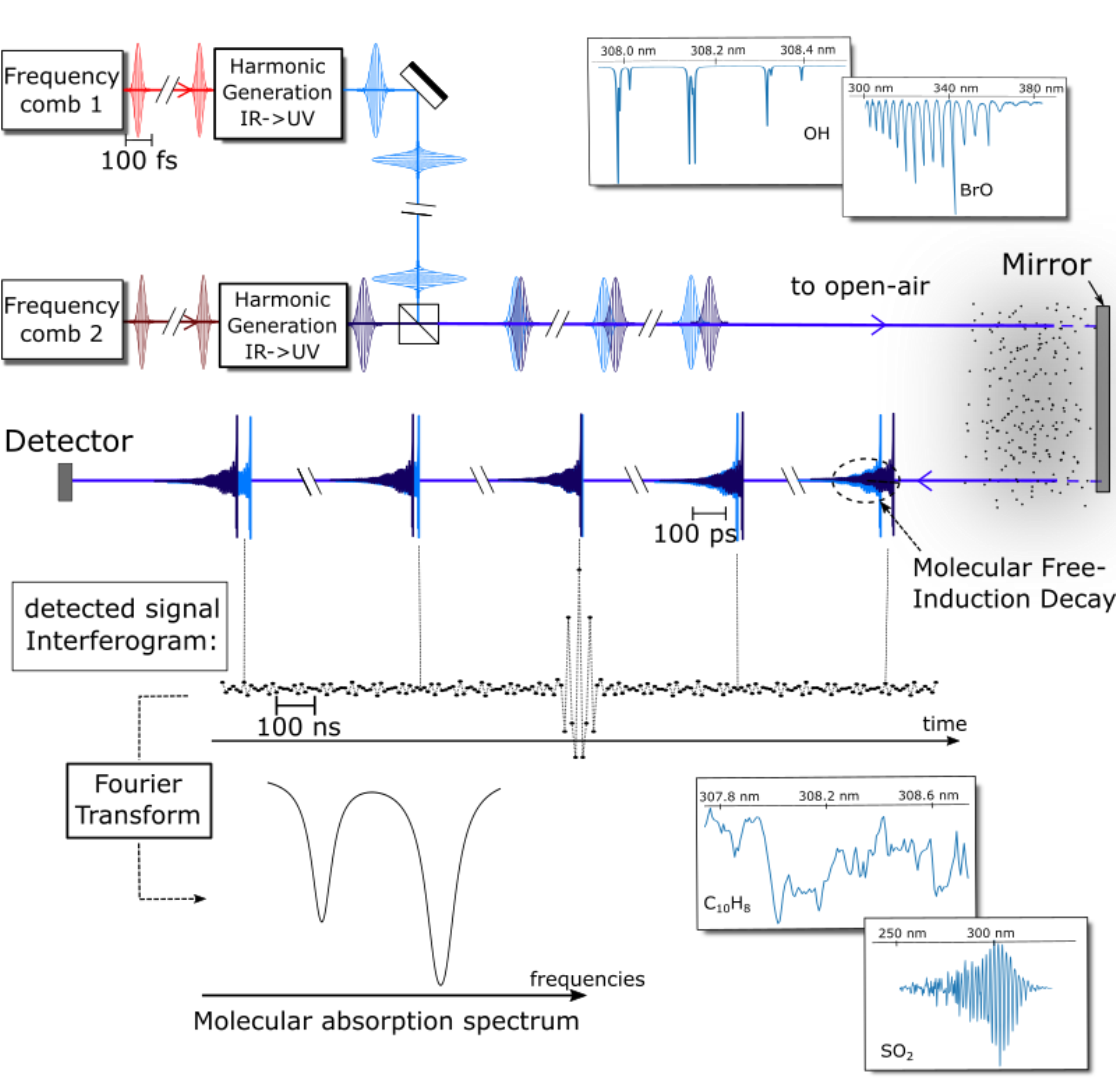
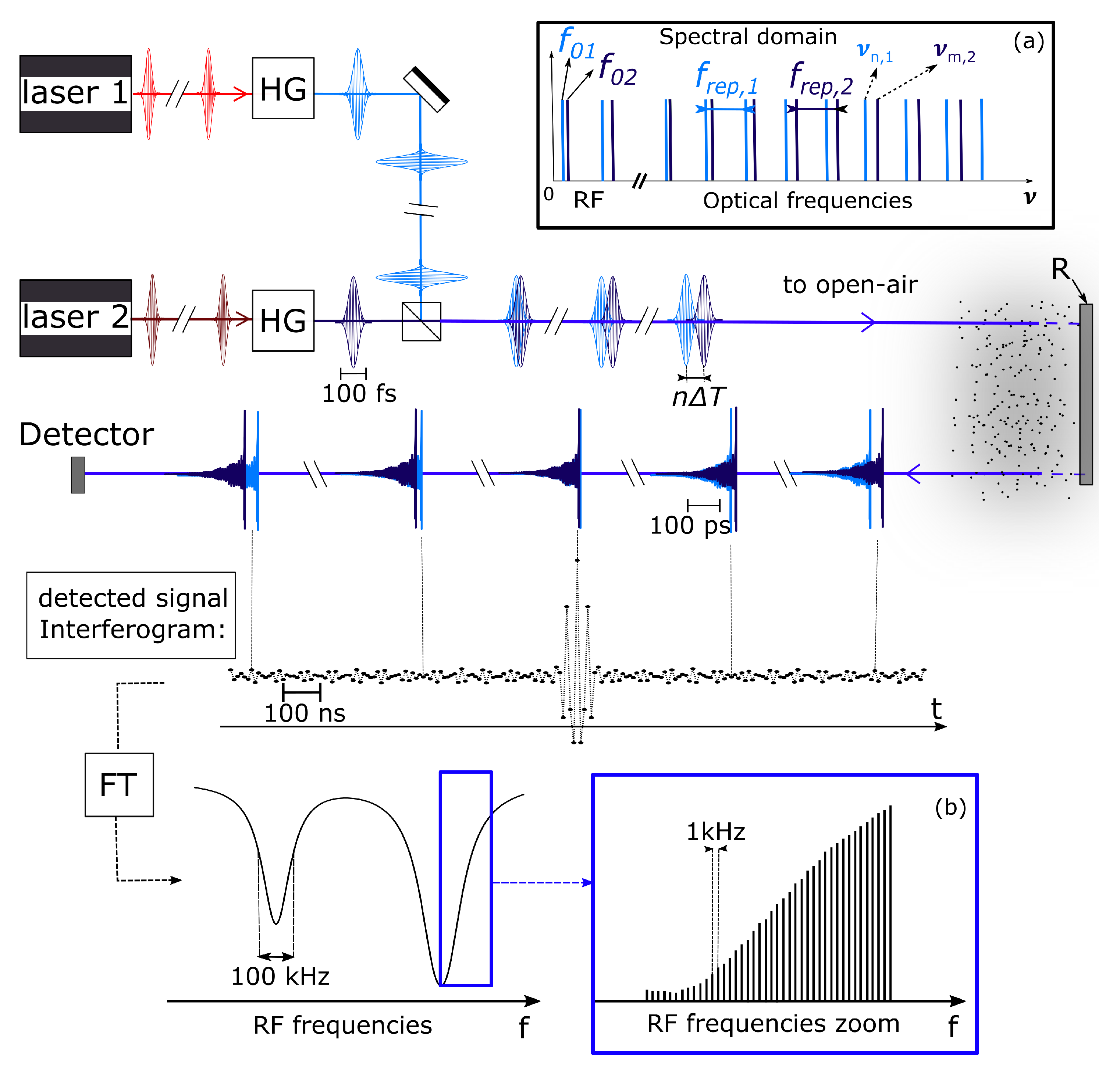
Dual-Comb spectroscopy was first proposed by Keilmann, van der Weide, and co-workers in 2004 as a “time-domain frequency-comb spectrometer” [33,34]. We here briefly present the principles of DCS and the quantities relevant for our study. A detailed description of DCS can be found, for example, in the review of Coddington et al. [30]. DCS is based on a Fourier transform spectrometer creating interference patterns between two mode-locked femtosecond pulsed lasers. A mode-locked fs laser can generate in the spectral domain a very broad and structured spectra composed of regularly spaced optical frequencies (see Figure 1, inset(a)). The frequency of each optical mode can be related to the radio-frequencies , the laser pulse emission repetition frequency, and , an offset frequency, so that:
where n is an integer in the order of . results from the different carrier and envelop velocities of the fs pulses inside the laser cavity. If the radio-frequencies are well determined, Equation (1) gives an unambiguous relation between radio-frequencies (, ) and the optical frequencies () of the laser emission. Such a laser emission spectrum is called a comb with equally spaced teeth and has revolutionized high-resolution metrology in the optical domain [35,36,37].
The two Optical Frequency Combs (OFC), labelled (1) and (2), used for Dual-Comb Spectroscopy have a slightly different repetition frequency: (typically from a few Hertz to a few kHz). For ease of reading, we will set . In the time frame, this stable frequency difference creates a coherent femtosecond time-delay between the pulses of the two lasers with a time step of (typically tens of femtoseconds). During their propagation in the atmosphere, one can say that the pulses of the first laser walk through the pulses of the second laser. This creates the optical scanning delay required for any FTS-type experiment. Unlike conventional FTS, the DCS time-scanning procedure is free from any mechanical moving parts, and attains scanning velocities 3 or 4 orders of magnitude faster than conventional FT due to the down-conversion to RF frequencies instead of acoustic frequencies. A simulated DCS interferogram is illustrated in Figure 1. The center-burst of this interferogram represents the exact temporal superposition of a light pulse from each laser. As the light pulses propagate through an absorbing medium, their temporal shape is imprinted by the Free-Induction Decay (FID) of the excited molecular levels, interfering with the light source. This decay time is set by collisions and Doppler dephasing (spectral broadening). For standard thermodynamic conditions, the width of molecular line shapes is a few GHz which translates into an FID decay time of hundreds of picoseconds.
In the laboratory frame, the time-increment of the interferogram is given by and is of the order of tens of nanoseconds and produces the stroboscopic effect essential for measuring such short decays. Finally, by performing a numerical Fourier transformation on the acquired interferogram, the modified spectrum of the light sources which has been imprinted by the absorption lines of the interfering molecules is recovered. The RF-to-optical spectral mapping is ensured using the scaling factor . To prevent any spectrum aliasing effect, the () combination must be chosen so that the detected optical spectrum width is smaller than the aliasing-free spectral range of DCS as calculated, in the optical domain, by .
2.2. UV-DCS Spectrometer Signal Fluctuations
In this section, the different contributions to the interferogram signal fluctuations are presented to allow a comprehensive study on their impact on the minimal absorption sensitivity (MAS) described in Section 5.1. The temporal SNR, SNRt, of a DCS interferogram represents the amplitude of the center burst over the standard deviation of the signal far away from the center burst (see Figure 1). The spectral SNR, SNRf represents the amplitude of the intensity spectral density versus its standard deviation. represents the noise standard deviation given as 1/ SNRf for normalized amplitudes. The sources of noise on the interferogram can be subdivided into three contributions: (i) intrinsic amplitude and phase noise of the light source; (ii) amplitude and phase noise imprinted by atmospheric turbulences on to the light source; and (iii) detection noise.
The intrinsic amplitude noise of the light source is quantified by the relative intensity noise (RIN). The RIN of the laser source of mean intensity represents the power spectral density (PSD) of , where represents the root–mean–square (RMS) of the amplitude fluctuations of the normalized amplitudes.
The intrinsic optical phase noise (or carrier phase noise) of the OFC is linked to frequency fluctuations in the position of the OFC modes. If is the PSD of these frequency fluctuations at Fourier frequency f, the PSD of the optical phase noise of mode n is . The accumulated RMS phase noise within the interval of Fourier frequencies [] is then estimated as . In this study, the highest characteristic Fourier frequency is the Nyquist frequency ( MHz ) and the lowest Fourier frequency is majorized by the inverse of the duration of an individual interferogram ( kHz). The coherence time is generally defined as the time-scale over which the accumulates 1 rad, and it is estimated for potential candidate for UV-OFC laser sources in Section 3. Phase noises lower than 1 rad that could not have been removed by phase-locking stabilization protocols are called residual phase noises.
The influence of atmospheric turbulence into the signal is discussed in Section 4. We show that the contribution of atmospheric turbulences can be neglected below 100 s time scales, and this sets an upper limit for the acquisition time of a single interferogram.
Detector noise is quantified by the Noise Equivalent Power (NEP) of the detector. Expressed as dBc/, it takes into account the thermal noise and the dark current noise. At such short time scales, the detection noise is considered as white noise.
We now recall the formalism of the signal/noise ratio attainable with a Dual-Comb spectrometer, as introduced by Newbury et al. [38]. We consider the case of a single detector without optical filters. Taking into account the different noise contributions, takes the form:
From left to right, the terms in brackets represent the detector NEP contribution, the detector shot noise contribution, the RIN contribution, and the limitation of the SNR due to the dynamic range D of the measurement limited by either the acquisition card or the detector. is the average OFC power, T the total acquisition time (), h the Planck constant, the optical frequency of the light pulses, and the quantum efficiency of the detector. The factor b takes value 1 (or 2) for balanced (or unbalanced) detection. The noise scales linearly with the number of resolved spectra element , where is the optical spectral width of the OFC that can be simultaneously recorded and is the resolution of the DCS spectrometer.
However, the spectral resolution is often limited by the coherence time of the two combs that is usually shorter than a single interferogram total duration, . In the former case, is lower than and the resolution can be much greater than . Moreover, the temporal truncation of the individual interferograms creates a measurement dead-time that is taken into account by the introduction of the duty cycle factor . To estimate realistic contributions to the noise budget in the specific context of UV-DCS, we consider next the performances of possible UV sources.
3. UV-DCS Laser Sources
The development of DCS in the UV range is conditioned by the availability of two frequency combs operating in the UV range. Today, UV-OFC can only be generated by nonlinear up-conversion from an IR-OFC. The two main challenges of performing DCS in the UV range is to produce sufficient UV power at the full repetition-rate of the IR frequency comb and to recover the mutual coherence of the two UV-OFCs to obtain a high SNR. A UV frequency comb has already been realized at a full repetition rate for high-resolution spectroscopy of the 1S–3S transition in hydrogen [39]. However, neither the optical phase noise nor RIN, specifically at short time scale s, were reported. Therefore, to calculate the performances of UV-DCS, the optical phase noise and RIN transferred from IR sources to the UV spectral range need to be estimated.
There are three well-established strategies to generate UV-OFC: first, supercontinuum broadening in micro-structured fibers, second, high harmonic generation (HHG) in noble gases and third, harmonic generation in bulk crystals. To retain the phase coherence of the fundamental laser in the UV range, only the second and third strategy are appropriate here [40], and only the third is likely to yield the high power needed for remote-sensing applications. The PSD of the optical phase noise is quadratic in harmonic order k leading to a linear increase of the optical phase noise RMS with k [41]. Verification of the coherence transfer in bulk crystals has been demonstrated experimentally in a DCS type experiment [42]. Phase noise is usually quoted in the literature but not relative phase noise between two combs. However, using stabilization protocols, relative phase noise on the same level of individual phase noise has been achieved [43]. In addition, post-processing protocols or real-time monitoring can be used to correct for the relative frequency jitter of the sources [44]. The power of the up-converted beam is quadratic in the input optical power. This means that the RMS of the relative intensity fluctuations of the kth harmonic is expected to be a factor k higher leading to an RIN (PSD), a factor higher than the fundamental RIN. This law has been experimentally demonstrated for SHG in bulk crystals [45,46].
As shown in Section 5.1, the minimum detected UV power to realize a high SNR measurement is on the order of 1 mW. Given the strong atmospheric extinction in the UV range, a UV-DCS source suitable for remote-sensing application will require output power higher than 10 mW for a typical propagation path of 5 km. The UV-DCS light source must be coherent over a characteristic time scale of 100 s and present the lowest possible relative intensity noise. As stated previously, we envisage a UV-OFC that can meet the following specifications: (Case 1) an optical spectrum centered around 308 nm of spectral width 1 THz (0.3 nm, 33 cm−1), and/or (Case 2) an optical spectrum centered from 300 nm to 400 nm with a spectral width of at least 50 THz (20 nm, 1730 cm−1) (see Figure 2).
Erbium-fiber lasers show phase coherence that can meet the specifications. Based on reported coherences in the fundamental [47], we estimate that over the time-scale of one interferogram (s), the phase noise of the 4th (390 nm) or the 5th (312 nm) harmonic stays lower than 1 rad. Via the generation of the 4th harmonic, 6 mW of 1 ps laser has been reported [48]. We can note the generation of 250 mW UV beam in periodically poled crystals [49], but the reported spectral bandwidth of 0.1 nm is not appropriate for atmospheric studies. However, the developments of such a source in the UV open the way for applications requiring less optical power or less optical bandwidth in laboratory studies. This is also true for UV-DCS with Ytterbium-fiber lasers for which a proof of principle UV-DCS has been reported in a laboratory at 350 nm via high harmonic generation [50]. The feasibility of UV-DCS using fiber lasers for laboratory studies has been addressed elsewhere [51].
Titanium-sapphire lasers (TiSa) have specifications that could allow UV-DCS remote sensing applications considering their IR output power, spectral width, and coherence performances. TiSa lasers emit from 600 to 1100 nm allowing efficient VUV generation via SHG or THG. Devices to frequency double and triple cw mode-locked TiSa lasers are commercially available with efficiencies ranging from 20 to 50% for SHG and from 3 to 15% for THG. High blue radiation powers have been reported via direct SHG or THG (SHG: 625 mW–220 fs, THG: 150 mW–260 fs) [52].
High doubling efficiency has been demonstrated using BiB3O6 (BIBO) crystal (SHG: 830 mW–220 fs) [53,54].
The lowest optical phase noise of a TiSa frequency comb tooth has been achieved by phase-locking a comb tooth to an etalon optical source at 698 nm [55] or 657 nm [56]. From the work of Quraishi et al. [56], we estimated the relative accumulated optical phase noise of OFC to be lower than 0.5 rad in the Fourier frequency range [10–50 MHz]. Accumulated optical phase noise values have been reported from 10 kHz to 100 kHz. For higher Fourier frequencies, the phase noise reaches the shot noise level and its contribution is negligible. Coherence is therefore maintained over a single interferogram after SHG from the initial OFC. Sutyrin et al. [55] reported an accumulated phase noise of 0.11 rad from 10 kHz to 100 kHz Fourier frequencies for the reference tooth. The frequency noise at another comb tooth can be estimated using Equation (A1). Up to a spectral width of 40 nm (26 THz) in the fundamental IR, we estimate that the phase noise PSD of the furthest comb tooth will be comparable to the phase noise PSD of the reference comb tooth. Therefore, we predict an accumulated phase noise of 0.33 rad from 10 kHz to ≈ 50 MHz in the UV range via THG. This allows UV-DC spectroscopy with limited SNR reduction due to residual phase errors. Moreover, such a level of accumulated phase noise is maintained during at least 130 ms, allowing coherent averaging protocols that drastically reduce analysis time [57].
We now assess the RIN level of a UV-OFC generated from a TiSa laser. The contributions to the RIN as a function of Fourier frequencies usually include a peak corresponding to the laser relaxation oscillation, around hundreds of kHz for TiSa. Above 1 MHz, the RIN tends toward the shot noise limit of the detection system. We decided to use an upper limit for the RIN, assumed constant. RIN values between −135 dBc/Hz, and −140 dBc/Hz have been reported in TiSa, from studies comparing different pump lasers [46,55,58]. Taking the highest of these RIN values, we estimate a RIN of −129 dB/Hz for SHG and −125 dB/Hz for THG.
The benefit of using a TiSa oscillator for remote-sensing UV-DCS is two-fold: it requires only low-harmonic generation to reach UV range, resulting in a higher available power and with limited phase-noise degradation. Moreover, its spectral coverage appears relevant for atmospheric trace gases.
4. UV Light Propagation into the Atmosphere
Short-scale atmospheric turbulence (millimeters to meters) perturbs the propagation of a UV frequency comb by adding phase and amplitude noises to the UV radiation. This can significantly affect the sensitivity of the UV-DCS experiment. Temperature fluctuations (0.1° to 1°) caused by the turbulent motion of the atmosphere induce local refractive index fluctuations in the order of . The interaction of an electromagnetic wave with a single refractive index fluctuation (acting as a scatterer) results in phase fluctuations and amplitude fluctuation (or speckle). Phase fluctuations translate into beam wander, timing jitter (first-order), and to pulse broadening (second-order) [59]. Atmospheric turbulences are therefore a major concern for open-air measurements. Previous DCS demonstrations in the IR range show that the turbulences of the atmosphere did not alter the interferogram pattern because the acquisition time of the interferogram is shorter than the characteristic time of atmospheric turbulence: within the DCS acquisition time, the atmospheric turbulence appears to be frozen [24]. Because the atmosphere-induced noises depend on the wavelength of the light source, in the following, we estimate the level of immunity of UV-DCS to atmospheric turbulence. From the laws of diffraction, the amplitude of the scattered wave increases as wavelength decreases: phase and amplitude fluctuations are likewise greater in the UV range.
4.1. Atmosphere-Induced Amplitude Noise
Because of the fast acquisition rate of DCS, it is necessary to estimate the atmospheric-induced amplitude noise at fast Fourier frequencies. Very few experimental measurements have been performed in the UV range. In the context of trace gas detection, Armeding et al. measured the atmospheric transmission noise at 308 nm as imprinted by the intensity fluctuations, to be on a maximum level of (rms) for a single s scan [60]. Under the hypothesis of random noise, an averaging time of 1 s can reduce the atmospheric contribution to the overall noise to a level of as required for trace gas detection. Dual-Comb spectroscopy does offer fast acquisition times on the order of hundreds of microseconds. A s interferogram leads to a 1 GHz spectral resolution (see Section 2.1), sufficient to resolve—for example, the 7.9 GHz Lorentzian width of the OH molecule absorption lines at ambient pressure and temperature conditions.
Using the theoretical Kolmogorov spectrum of the spectral density for the refractive index fluctuation and the Taylor’s frozen-in hypothesis [59]: the power spectral density of the intensity noise due to atmospheric turbulences falls off as beyond the cut-off frequency, . For a wind speed of U = 5 m/s, a path length L = 5 km, = 300 nm, the cut-off frequency is Hz (7 ms). Therefore, as long as the refresh rate of the interferogram () is well above the cut-off frequency, the atmosphere-induced intensity noise is frozen during the acquisition time of a single interferogram. We assumed 100 s for the time truncation of a single interferogram for a safe estimation of the frozen atmosphere hypothesis. It can be noticed, as underlined by Rieker et al. [24] that although the acquisition frequency is higher than the cut-off frequency, the intensity noise that remains on a time scale of one interferogram could induce multiplicative noise. This multiplicative noise may limit the achievable detection limit but has appeared negligible in remote-sensing IR-DCS [24]. As such, the source of noise is highly dependent on the atmospheric turbulence structure , an experimental approach seems to be the way to quantify its contribution for UV-DCS and is thereby out of the scope of this paper.
4.2. Atmosphere-Induced Phase Noise
Phase noise induces jitter noise (pulse-to-pulse arrival time) that would decrease the coherence time of the experiment. Our concern is phase noise on a time scale shorter than which behave exactly as the amplitude spectral density [59]. Phase noise can be related to timing-jitter noise by , where is the carrier optical frequency. We estimate an atmospheric-induced phase noise of –70 dBc using the same atmospheric parameters as for the calculation of atmospheric-induced amplitude noises. This value leads to a turbulence-induced timing-jitter noise at 10 kHz Fourier frequencies. The integrated timing jitter from 10 kHz to 100 MHz (pulse-to-pulse) is ≤ 1 fs, which is one order of magnitude lower than the temporal increments of one interferogram = 10 fs (with = 100 MHz and = 1 kHz). Moreover, in the co-propagating geometry, the two combs propagate in the same turbulent medium and therefore undergo similar phase distortions. Therefore, in this configuration, atmospheric-induced relative phase fluctuations are bound to be negligible compared to the inherent relative phase noise of the two UV-OFCs.
5. Results: Simulated UV-DCS Sensitivity
In this section, we calculate the performances of the here simulated UV-DCS remote-sensing spectrometer in terms of minimum detectable optical depth or Minimal Absorption Sensitivity (MAS). We first estimate the quality factor of the UV-DCS spectrometer defined as the signal/noise ratio per spectral element achieved with 1 s acquisition time (no dead-time). The quality factor allows for efficent comparison of performances of different spectrometry systems [38]. We consider that the UV-DCS spectrometer is coupled to a remote sensing optical device as depicted in Figure 1. Its precise technical arrangement needs precise parametrization of the laser (beam quality, divergence) and is out of scope of this numerical study. However, given a typical SHG or THG Gaussian TiSa laser beam divergence of 2 mrad, the optical sensing device would require at least a 50 times beam expander, a tens of centimeters diameter mirror-type reflector, sending and receiving optics and a telescope for the light collection in an off-axis arrangement. Fast-steering mirrors will be used for beam wandering correction over the typical time of the interferograms refresh-time. Numerical data are taken for existing TiSa laser sources with their specifications in terms of RIN, repetition rate, and optical spectral coverage (see Table 1). is fixed to 100 MHz as state-of-the-art low phase noise lasers operate around this repetition frequency. We then conclude on the detection limit of the targeted trace gases.
5.1. Quality Factor and Minimum Absorption Sensitivity
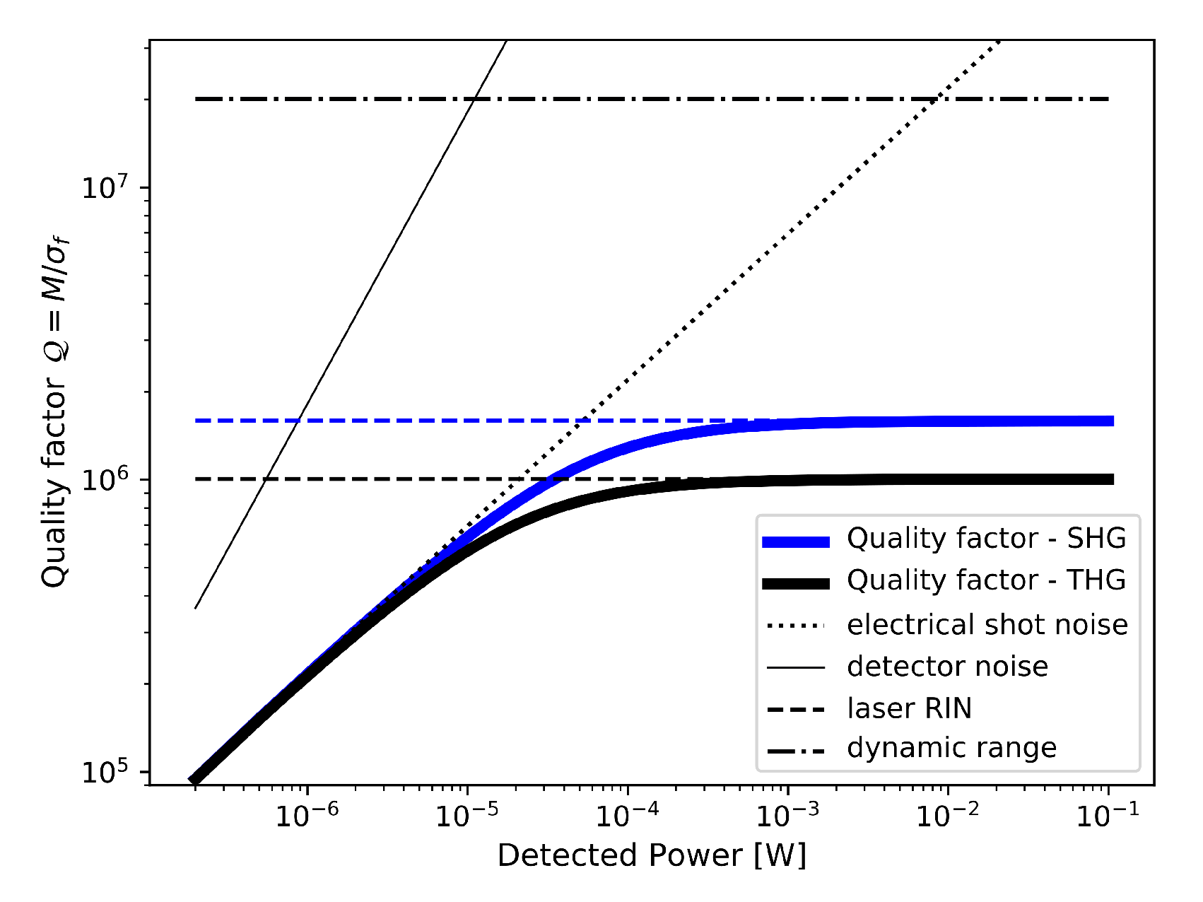
Using the parameters of Table 1, the quality factor for UV-DCS when using the second and the third harmonic of a TiSa laser as the UV source is illustrated in Figure 3. Our calculations show that the UV-DCS quality factor is approximatively a factor of 6 lower than IR-DCS [38]. The main reason for this strong decrease is the lower RIN value for UV-DCS. The predominant noise at low detected power is the detection shot noise, for detected power higher than 1 mW, the SNR is laser-RIN limited and reaches its maximum value. Different types of detector have been envisaged: avalanche, amplified, biased photodiodes or Super Bilakali Photomultipliers. For each detectors, neither their NEP value nor their dynamic range would limit the SNR. Therefore, the best detector choice appears here to be the biased photodiode for its highest saturation power, allowing mW detection power for best SNR. The reduction of the SNR due to the residual phase noise is described in Appendix A and is taken into account in all the SNR analysis.
To evaluate the minimum absorption sensitivity (MAS), one should consider, in addition to the molecular spectroscopic parameters, the quality factor previously evaluated, with proper M and duty-cycle factor values. The MAS, adapted from [38], is defined as twice the SNR:
where is the peak absorption coefficient of the considered molecular line, L the absorption light path and is an enhancement factor due to the high spectral resolution of DCS. The sum is over the different molecular absorption lines with individual Lorentzian FWHM and peak absorption . is typically between 0.1 and 1 depending on the width of the spectral line and the resolution of the experiment. accounts for the geometry of the spectrometer. In our study, the absorbing medium is probed by the two laser beams for atmosphere-induced phase noise reduction (see Section 4). The sensitivity is therefore enhanced by a factor of two () compared to the geometry in which the absorbing medium is probed by a unique source.
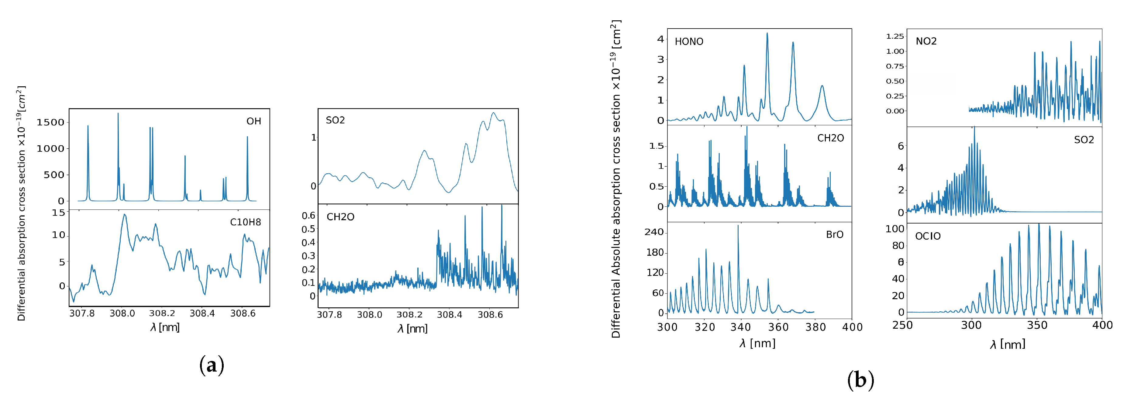
In the following, we present MAS evaluations for the two different case studies. MAS values are calculated considering Equation (3) and taking into account the influence of residual phase noise (see Appendix A). Note that some absorbing species can be detected both in Cases (1) and (2) as illustrated for formaldehyde and sulphur dioxide. The peak absorption coefficients are estimated using the differential absorption cross-sections of the targeted gases (see Figure 2). The differential absorption cross-sections are composed of the fastest varying absorption features and their use is essential during the gas concentration retrieval procedure to separate the molecular spectral signature from the slow varying Rayleigh scattering or aerosol extinction [6].
5.2. Case (1): 308 nm: Narrow Spectral Range and High Spectral Resolution
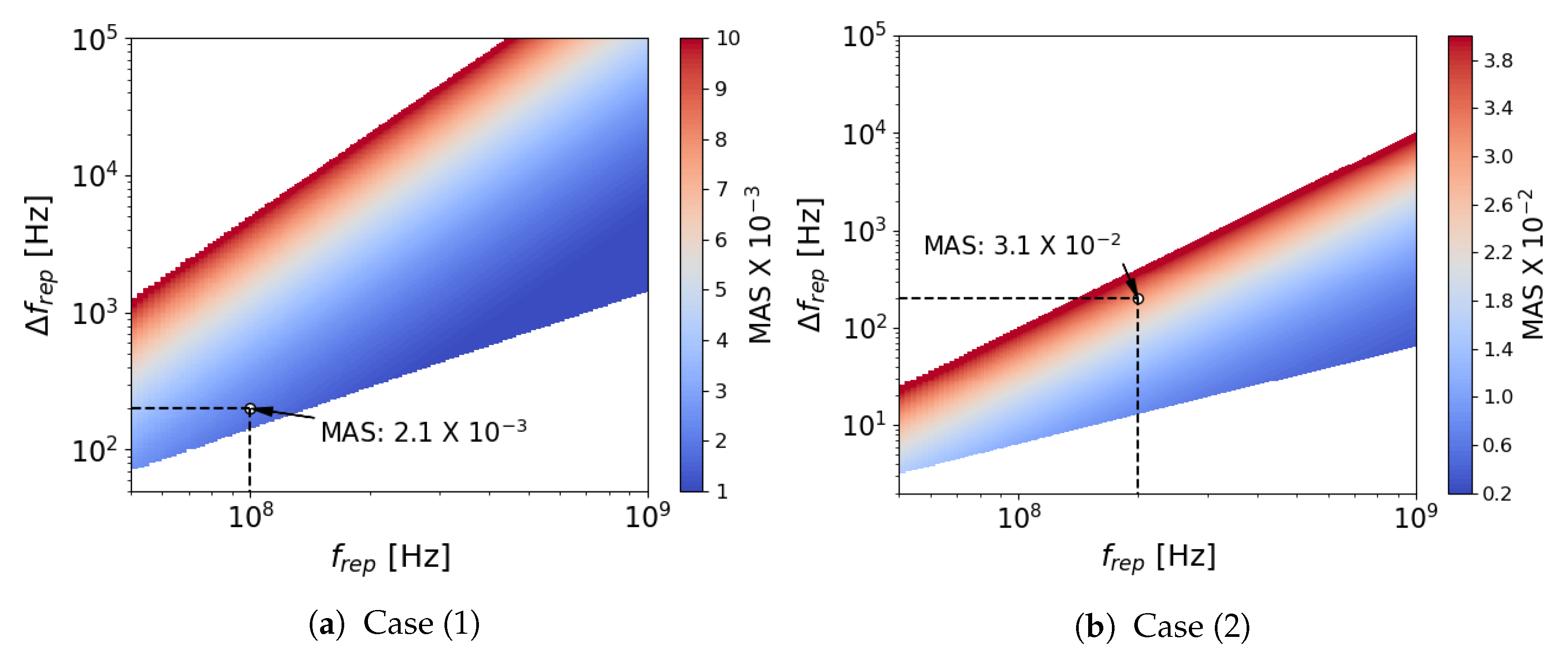
For case-study (1), we consider a UV-OFC at 308 nm generated by tripling the fundamental 924 nm radiation of TiSa. The RIN value used in Case (1) is −125 dBc/Hz as we estimated for THG (see Section 3). The achievable MAS for different combinations are represented in Figure 4a, and summarized for typical couples of values in Table 2. OH radical shows well separated absorption lines, with a lorentzien width of 7.9 GHz (see Figure 2a). The sensitivity enhancement has been estimated at the line which presents the highest cross-section and worth 1/2 to 1/7 depending on the value .
5.3. Case (2): 350 nm: Broad Spectral Range and Low Spectral Resolution
Case (2) requires the use of blue sub-20 fs radiation. Such ultra-short and near-Fourier limited UV pulses have been successfully generated via SHG from TiSa using intra or extra cavity schemes [61,62,63]. The RIN value estimated in Case (2) is −129 dBc/Hz. The spectral resolution can be set up to 0.03 nm (77 GHz). To verify the aliasing-free spectrum requirement for such a broad spectral range, the use of a larger value would relax the condition on . However, it is expected that the phase coherence of the OFC source is degraded at a higher repetition rate. The achievable MAS for different combinations are illustrated in Figure 4b and examples using values from experimental realizations are listed in Table 2. The low duty cycle and the large optical bandwidth explain the lower sensitivity of Case (2) compared to Case (1). The use of optical filters to perform a sequential filtering has been proposed as a strategy to improve the SNR [38]. However, considering the large molecular spectral line-width in Case (2), the multiplicative noise is expected to exceed the additive noise when reducing the spectral coverage of individual measurements (see Appendix A).
5.4. Results on Concentration Detection Limits
Simulations of trace gas concentration detection limits have been performed by considering a light path of 2 km into the atmosphere and an acquisition time of 200 s (see Table 3). The chosen averaging time and absorption light path are typical values for actual open-path spectroscopy experiments (DOAS).
6. Discussion
For both case-studies, the simulated MAS results are achievable if phase-corrected interferograms can be averaged. For UV-DCS, the SNR at 100 s is approximatively 5 for Case (1) and below 1 for Case (2) which prevents direct phase correction or summed FT spectra. However, we estimated that the coherence is maintained during longer acquisition time, up to 130 ms. This allows the use of coherent averaging protocols as proposed by Coddington et al. [57] for approximatively ten interferograms. The summed interferograms can be then averaged out after usual phase correction [7]. The conditions of such a correction is either a high signal/noise ratio for the summed interferograms or a monitoring of , and of the slow OFC amplitude fluctuations. Real-time adaptative sampling can also be considered [44]. Longer acquisition time can be achievable using consecutive similar schemes. In practice, the averaging time is limited by buffer size considerations and acceptable processing times.
The predicted concentration detection limit of OH with UV-DCS is 0.08 ppt ( molec./cm3-MAS of 7 at 200 s acquisition time). MAS of 1 are reported in the literature by active or passive DOAS or MOAS (Multipass Optical Absorption Spectroscopy) with similar averaging time. To match this performance and with the actual laser light sources, UV-DCS would require 2.7 h of averaging time, which is incompatible with atmospheric trace gases monitoring. However, the UV-DCS predicted concentration limit for OH of 0.08 ppt allows the remote evaluation of ambient OH concentration in various environments, from pristine to urban during the daytime (typical concentration of 0.3 ppt [64]).
Such level of sensitivities could make possible the remote detection of highly concentrated OH environments using UV-DCS as, for example, in combustion diagnostics. For this application, the fast acquisition time of UV-DCS could be relevant to monitor combustion dynamics.
The estimated performances of UV-DCS in Case (2) appear competitive with the performances reported in the literature. In Case (2), DCS takes advantage of its large spectral coverage in short acquisition time. Comparison with up-to-date experiments shows that UV-DCS outperforms the reported sensitivity of UV-FTS experiment for both case studies (see Table 4). DOAS type experiments show better sensitivities for Case (1) and similar sensitivities for Case (2). The limiting factor of UV-DCS being the RIN value, we believe that this parameter can be improved using pulse-to-pulse monitoring of the amplitude of femtosecond pulses.
7. Conclusions
The present paper shows that UV-DCS offers, by its fast acquisition rate, the required immunity to atmospheric turbulence for trace-gas concentration monitoring in the atmosphere. A TiSa based UV-DCS appears to be the most relevant fs light source for remotely probe atmospheric molecules in the UV range. UV-DCS allows the multi-trace detection that is necessary for trace gases remote sensing. We show that the sensitivity of the UV-DCS spectroscopy is primarily limited by the RIN level of the UV source. We estimate that UV-DCS with current UV-sources do not surpass open-path optical differential absorption spectroscopy in terms of sensitivity, but should be comparable in situations where a wide optical spectral bandwidth is necessary. UV-DCS could therefore contribute to mitigating the lack of open-path and broadband experiments in the UV range to address the highly reactive molecules of the atmosphere. A pulse-to-pulse monitoring of the amplitude fluctuations would be a prerequisite for any sensitivity improvement. Another limitation of atmospheric UV remote-sensing sensitivity is the precision of the molecular spectroscopic reference data which have not been addressed in this study. This investigation is a preliminary to experimental verification of several aspects, notably the atmosphere-induced multiplicative noise that can reduce the achievable detection limit, and the retrieval of the high SNR using the cited averaging strategies. We believe that this study provides a first framework for future experimental demonstrations of trace-gas remote detection in the UV range using DCS.
Author Contributions
Conceptualization, S.G. and P.R.; Data curation, S.G. and C.P.; Formal analysis, S.G. and C.P.; Funding acquisition, S.G. and P.R.; Investigation, S.G. and C.P.; Methodology, S.G., C.P. and P.R.; Project administration, S.G. and P.R.; Software, S.G. and C.P.; Supervision, S.G. and P.R.; Validation, S.G. and P.R.; Visualization, S.G. and C.P.; Writing—original draft, S.G., C.P. and P.R. All authors have read and agreed to the published version of the manuscript.
Funding
This research was funded by the CNRS-EMERGENCE 2017 project and FRAMA—University of Lyon.
Conflicts of Interest
The authors declare no conflict of interest. The funders had no role in the design of the study; in the collection, analyses, or interpretation of data; in the writing of the manuscript, or in the decision to publish the results.
Abbreviations
The following abbreviations are used in this manuscript:
| DCS | Dual-Comb Spectroscopy |
| OFC | Optical Frequency Comb |
| SNR | Signal/Noise Ratio |
| PSD | Power Spectral Density |
| RIN | Relative Intensity Noise |
| NEP | Noise Equivalent Power |
| IGM | Interferogram |
| MAS | Minimum Absorption Sensitivity |
| DOAS | Differential Optical Absorption Spectroscopy |
| MOAS | Multipass Optical Absorption Spectroscopy |
Appendix A. Multiplicative Noise Due to Residual Relative Optical Phase Noise
According to the “comb” Equation (1), the optical phase noise PSD of comb mode n, , arises from frequency fluctuations in the repetition rate frequency (associated with timing phase jitter, resulting in fluctuations of the pulse-to-pulse arrival time), and from frequency fluctuations on the carrier-envelope offset frequency . The repetition rate frequency can be easily locked and stabilized to reach its quantum limit, but the stabilization of is more challenging. Low optical phase noise OFCs use active feedback loop to stabilize and via either a radio frequency reference or an optical etalon. For a comb tooth phase locked to an optical etalon, the optical phase PSD of the comb mode n is given by:
where and represent the phase noise PSD of the optical phase of comb number and carrier envelope phase offset, respectively.
The phase noise RMS , squared, is obtained by integration of from the inverse of the observation time to an upper limit frequency of 50 MHz. The values reported by Sutyrin et al. [55] are used and we verified that the contribution of the noise at Fourier frequencies higher than 1 MHz to the overall noise is negligible. The fast phase noise RMS corresponds to an observation time of 100 ms. The slow phase noise has been calculated using an observation time of 130 ms, the longest reported observation time for the optical phase noise in reference [55].
Because of the existence of residual phase noise over time-scales longer than the duration of a single interferogram, , the SNR of the averaged interferogram is reduced by the factor [38]. For Case (1), the residual phase noise is estimated to be approximatively 0.33 rad, which leads to a reduction of the SNR by 6.5%. For Case (2), the SNR is reduced by 2.4% (SHG instead of THG). Such reduction factors are taken into account in all our simulations.
For the two case studies, we estimated , the contribution of the multiplicative noise to the noise across a molecular absorption spectral line of width due to the existence of residual phase noise over the duration of a single interferogram [38]. This contribution takes the form:
Table A1 reports our estimations of the multiplication noise for the trace gases of our study. We calculate that, for all case studies, the multiplicative noise across the targeted molecular lines does not exceed the additive noise .

Table A1.
Comparison between additive and multiplicative noise using with 1 s acquisition time. Case (1): = 0.33 rad, = 1 THz, = 100 MHz, Case (2): = 0.22 rad, = 50 THz, = 200 MHz. corresponds to the standard deviation of the noise considering only the additive sources of noise, as calculated via Equation (2).
| Case Study | Components | |||
|---|---|---|---|---|
| Case (1) | ||||
| OH | 1 / 111 | 8.9 | 1 | |
| Naphthalene | 1/ 33 | 3 | 2 | |
| Formaldehyde | 1/ 33 | 3 | 2 | |
| SO2 | 1/ 22 | 5 | 2 | |
| Case (2) | ||||
| BrO/Formaldehyde | 1/25 | 9.3 | 3 |
References
- Wei, Y.; Wang, Y.; Wu, X.; Di, Q.; Shi, L.; Koutrakis, P.; Zanobetti, A.; Dominici, F.; Schwartz, J.D. Causal Effects of Air Pollution on Mortality in Massachusetts. Am. J. Epidemiol. 2020. [Google Scholar] [CrossRef] [PubMed]
- Hodgkinson, J.; Tatam, R.P. Optical gas sensing: A review. Meas. Sci. Technol. 2012, 24, 012004. [Google Scholar] [CrossRef] [Green Version]
- Shutler, J.D.; Quartly, G.D.; Donlon, C.J.; Sathyendranath, S.; Platt, T.; Chapron, B.; Johannessen, J.A.; Girard-Ardhuin, F.; Nightingale, P.D.; Woolf, D.K.; et al. Progress in satellite remote sensing for studying physical processes at the ocean surface and its borders with the atmosphere and sea ice. Prog. Phys. Geogr. Earth Environ. 2016, 40, 215–246. [Google Scholar] [CrossRef] [Green Version]
- Heymann, J.; Reuter, M.; Buchwitz, M.; Schneising, O.; Bovensmann, H.; Burrows, J.P.; Massart, S.; Kaiser, J.W.; Crisp, D. CO2 emission of Indonesian fires in 2015 estimated from satellite-derived atmospheric CO2 concentrations. Geophys. Res. Lett. 2017, 44, 1537–1544. [Google Scholar] [CrossRef]
- Bousquet, P.; Pierangelo, C.; Bacour, C.; Marshall, J.; Peylin, P.; Ayar, P.V.; Ehret, G.; Bréon, F.M.; Chevallier, F.; Crevoisier, C.; et al. Error Budget of the MEthane Remote LIdar missioN and Its Impact on the Uncertainties of the Global Methane Budget. J. Geophys. Res. Atmos. 2018, 123, 11,766–11,785. [Google Scholar] [CrossRef]
- Platt, U.; Stutz, J. Differential Optical Absorption Spectroscopy: Principles and Applications; Springer: Berlin/Heidelberg, Germnay, 2008. [Google Scholar] [CrossRef] [Green Version]
- Davis, S.P.; Abrams, M.C.; Brault, J.W. Fourier Transform Spectrometry; Academic Press: Cambridge, UK, 2001. [Google Scholar] [CrossRef]
- O’Keefe, A.; Deacon, D.A.G. Cavity ring-down optical spectrometer for absorption measurements using pulsed laser sources. Rev. Sci. Instrum. 1988, 59, 2544–2551. [Google Scholar] [CrossRef] [Green Version]
- Courtillot, I.; Morville, J.; Motto-Ros, V. Sub-ppb NO2 detection by optical feedback cavity-enhanced absorption spectroscopy with a blue diode laser. Appl. Phys. B 2006, 85, 407. [Google Scholar] [CrossRef]
- Crosson, E. A cavity ring-down analyzer for measuring atmospheric levels of methane, carbon dioxide, and water vapor. Appl. Phys. B 2008, 92, 403. [Google Scholar] [CrossRef]
- Megie, G. Laser Remote Sensing: Fundamentals and Applications. Eos, Trans. Am. Geophys. Union 1985, 66, 686. [Google Scholar] [CrossRef]
- Rossi, R.; Di Giovanni, D.; Malizia, A.; Gaudio, P. Measurements of Vehicle Pollutants in a High-Traffic Urban Area by a Multiwavelength Dial Approach: Correlation Between Two Different Motor Vehicle Pollutants. Atmosphere 2020, 11, 383. [Google Scholar] [CrossRef] [Green Version]
- Dubovik, O.; Holben, B.; Eck, T.F.; Smirnov, A.; Kaufman, Y.J.; King, M.D.; Tanré, D.; Slutsker, I. Variability of Absorption and Optical Properties of Key Aerosol Types Observed in Worldwide Locations. J. Atmos. Sci. 2002, 59, 590–608. [Google Scholar] [CrossRef]
- David, G.; Miffre, A.; Thomas, B.; Rairoux, P. Sensitive and accurate dual-wavelength UV-VIS polarization detector for optical remote sensing of tropospheric aerosols. Appl. Phys. B 2012, 108, 197–216. [Google Scholar] [CrossRef] [Green Version]
- Kolehmainen, M.; Martikainen, H.; Ruuskanen, J. Neural networks and periodic components used in air quality forecasting. Atmos. Environ. 2001, 35, 815–825. [Google Scholar] [CrossRef]
- Postolache, O.A.; Dias Pereira, J.M.; Silva Girao, P.M.B. Smart Sensors Network for Air Quality Monitoring Applications. IEEE Trans. Instrum. Meas. 2009, 58, 3253–3262. [Google Scholar] [CrossRef]
- Carnevale, C.; Finzi, G.; Pisoni, E.; Volta, M. Neuro-fuzzy and neural network systems for air quality control. Atmos. Environ. 2009, 43, 4811–4821. [Google Scholar] [CrossRef]
- Méjean, G.; Kassi, S.; Romanini, D. Measurement of reactive atmospheric species by ultraviolet cavity-enhanced spectroscopy with a mode-locked femtosecond laser. Opt. Lett. 2008, 33, 1231–1233. [Google Scholar] [CrossRef]
- Gherman, T.; Venables, D.S.; Vaughan, S.; Orphal, J.; Ruth, A.A. Incoherent Broadband Cavity-Enhanced Absorption Spectroscopy in the near-Ultraviolet: Application to HONO and NO2. Environ. Sci. Technol. 2008, 42, 890–895. [Google Scholar] [CrossRef]
- Amediek, A.; Ehret, G.; Fix, A.; Wirth, M.; Büdenbender, C.; Quatrevalet, M.; Kiemle, C.; Gerbig, C. CHARM-F—A new airborne integrated-path differential-absorption lidar for carbon dioxide and methane observations: Measurement performance and quantification of strong point source emissions. Appl. Opt. 2017, 56, 5182–5197. [Google Scholar] [CrossRef]
- Wagner, G.A.; Plusquellic, D.F. Ground-based, integrated path differential absorption LIDAR measurement of CO2, CH4, and H2O near 1.6 mu. Appl. Opt. 2016, 55, 6292–6310. [Google Scholar] [CrossRef]
- Rairoux, P.; Schillinger, H.; Niedermeier, S.; Rodriguez, M.; Ronneberger, F.; Sauerbrey, R.; Stein, B.; Waite, D.; Wedekind, C.; Wille, H.; et al. Remote sensing of the atmosphere using ultrashort laser pulses. Appl. Phys. B 2000, 71, 573–580. [Google Scholar] [CrossRef]
- Kasparian, J.; Rodriguez, M.; Méjean, G.; Yu, J.; Salmon, E.; Wille, H.; Bourayou, R.; Frey, S.; Andre, Y.B.; Mysyrowicz, A.; et al. White-light filaments for atmospheric analysis. Science 2003, 301, 61–64. [Google Scholar] [CrossRef] [PubMed]
- Rieker, G.B.; Giorgetta, F.R.; Swann, W.C.; Kofler, J.; Zolot, A.M.; Sinclair, L.C.; Baumann, E.; Cromer, C.; Petron, G.; Sweeney, C.; et al. Frequency-comb-based remote sensing of greenhouse gases over kilometer air paths. Optica 2014, 1, 290–298. [Google Scholar] [CrossRef]
- Schroeder, P.; Wright, R.; Coburn, S.; Sodergren, B.; Cossel, K.; Droste, S.; Truong, G.; Baumann, E.; Giorgetta, F.; Coddington, I.; et al. Dual frequency comb laser absorption spectroscopy in a 16 MW gas turbine exhaust. Proc. Combust. Inst. 2017, 36, 4565–4573. [Google Scholar] [CrossRef] [Green Version]
- Oudin, J.; Mohamed, A.K.; Hébert, P.J. IPDA LIDAR measurements on atmospheric CO2 and H2O using dual comb spectroscopy. Society of Photo-Optical Instrumentation Engineers (SPIE) Conference Series. In Proceedings of the International Conference on Space Optics-ICSO 2018, Chania, Greece, 9–12 October 2018; Volume 11180, p. 111802N. [Google Scholar] [CrossRef] [Green Version]
- Millot, G.; Pitois, S.; Yan, M.; Hovhannisyan, T.; Bendahmane, A.; Hänsch, T.W.; Picqué, N. Frequency-agile dual-comb spectroscopy. Nat. Photonics 2016, 10, 27–30. [Google Scholar] [CrossRef]
- Schubert, O.; Eisele, M.; Crozatier, V.; Forget, N.; Kaplan, D.; Huber, R. Rapid-scan acousto-optical delay line with 34 kHz scan rate and 15 as precision. Opt. Lett. 2013, 38, 1910–2907. [Google Scholar] [CrossRef] [Green Version]
- Baumann, E.; Giorgetta, F.R.; Swann, W.C.; Zolot, A.M.; Coddington, I.; Newbury, N.R. Spectroscopy of the methane ν3 band with an accurate midinfrared coherent dual-comb spectrometer. Phys. Rev. A 2011, 84, 062513. [Google Scholar] [CrossRef] [Green Version]
- Coddington, I.; Newbury, N.; Swann, W. Dual-comb spectroscopy. Optica 2016, 3, 414–426. [Google Scholar] [CrossRef] [Green Version]
- Picqué, N.; Hänsch, T.W. Frequency comb spectroscopy. Nat. Photonics 2019, 13, 146–157. [Google Scholar] [CrossRef]
- Meek, S.A.; Hipke, A.; Guelachvili, G.; Hänsch, T.W.; Picqué, N. Doppler-free Fourier transform spectroscopy. Opt. Lett. 2018, 43, 162–165. [Google Scholar] [CrossRef] [Green Version]
- Keilmann, F.; Gohle, C.; Holzwarth, R. Time-domain mid-infrared frequency-comb spectrometer. Opt. Lett. 2004, 29, 1542–1544. [Google Scholar] [CrossRef] [Green Version]
- Schliesser, A.; Brehm, M.; Keilmann, F.; Weide, D.W.V.D. Frequency-comb infrared spectrometer for rapid, remote chemical sensing. Opt. Express 2005, 13, 9029–9038. [Google Scholar] [CrossRef] [PubMed]
- Udem, T.; Holzwarth, R.; Hänsch, T.W. Optical frequency metrology. Nature 2002, 415, 233–237. [Google Scholar] [CrossRef] [PubMed]
- Hall, J.L. Nobel Lecture: Defining and measuring optical frequencies. Rev. Mod. Phys. 2006, 78, 1279–1295. [Google Scholar] [CrossRef] [Green Version]
- Hänsch, T.W. Nobel Lecture: Passion for precision. Rev. Mod. Phys. 2006, 78, 1297–1309. [Google Scholar] [CrossRef] [Green Version]
- Newbury, N.R.; Coddington, I.; Swann, W. Sensitivity of coherent dual-comb spectroscopy. Opt. Express 2010, 18, 7929–7945. [Google Scholar] [CrossRef]
- Peters, E.; Diddams, S.A.; Fendel, P.; Reinhardt, S.; Hänsch, T.W.; Udem, T. A deep-UV optical frequency comb at 205 nm. Opt. Express 2009, 17, 9183–9190. [Google Scholar] [CrossRef]
- Benko, C.; Allison, T.K.; Cingöz, A.; Hua, L.; Labaye, F.; Yost, D.C.; Ye, J. Extreme ultraviolet radiation with coherence time greater than 1 s. Nat. Photonics 2014, 8, 530–536. [Google Scholar] [CrossRef] [Green Version]
- Liehl, A.; Sulzer, P.; Fehrenbacher, D.; Rybka, T.; Seletskiy, D.V.; Leitenstorfer, A. Deterministic Nonlinear Transformations of Phase Noise in Quantum-Limited Frequency Combs. Phys. Rev. Lett. 2019, 122, 203902. [Google Scholar] [CrossRef] [Green Version]
- Ideguchi, T.; Poisson, A.; Guelachvili, G.; Hänsch, T.W.; Picqué, N. Adaptive dual-comb spectroscopy in the green region. Opt. Lett. 2012, 37, 4847–4849. [Google Scholar] [CrossRef] [Green Version]
- Coddington, I.; Swann, W.C.; Newbury, N.R. Coherent Multiheterodyne Spectroscopy Using Stabilized Optical Frequency Combs. Phys. Rev. Lett. 2008, 100, 013902. [Google Scholar] [CrossRef] [Green Version]
- Ideguchi, T.; Poisson, A.; Guelachvili, G.; Picqué, N.; Hänsch, T.W. Adaptive real-time dual-comb spectroscopy. Nat. Commun. 2014, 5, 3375. [Google Scholar] [CrossRef] [Green Version]
- Wang, Y.; Fonseca-Campos, J.; Liang, W.G.; Xu, C.Q.; Vargas-Baca, I. Noise Analysis of Second-Harmonic Generation in Undoped and MgO-Doped Periodically Poled Lithium Niobate. Adv. OptoElectron. 2008, 2008. [Google Scholar] [CrossRef] [Green Version]
- Tawfieq, M.; Hansen, A.K.; Jensen, O.B.; Marti, D.; Sumpf, B.; Andersen, P.E. Intensity Noise Transfer Through a Diode-Pumped Titanium Sapphire Laser System. IEEE J. Quantum. Electron. 2018, 54, 1–9. [Google Scholar] [CrossRef] [Green Version]
- Coddington, I.; Swann, W.C.; Newbury, N.R. Coherent linear optical sampling at 15 bits of resolution. Opt. Lett. 2009, 34, 2153. [Google Scholar] [CrossRef] [PubMed]
- Moutzouris, K.; Sotier, F.; Adler, F.; Leitenstorfer, A. Highly efficient second, third and fourth harmonic generation from a two-branch femtosecond erbium fiber source. Opt. Express 2006, 14, 1905–1912. [Google Scholar] [CrossRef]
- Kuzucu, O.; Wong, F.N.C.; Zelmon, D.E.; Hegde, S.M.; Roberts, T.D.; Battle, P. Generation of 250 mW narrowband pulsed ultraviolet light by frequency quadrupling of an amplified erbium-doped fiber laser. Opt. Lett. 2007, 32, 1290–1292. [Google Scholar] [CrossRef] [PubMed]
- Carlson, D.R. Frequency Combs for Spectroscopy in the Vacuum Ultraviolet. Ph.D. Thesis, University of Arizona, Tucson, Arizona, 2016. [Google Scholar]
- Schuster, V.; Liu, C.; Klas, R.; Dominguez, P.; Rothhardt, J.; Limpert, J.; Bernhardt, B. Towards Dual Comb Spectroscopy in the Ultraviolet Spectral Region. Available online: https://arxiv.org/abs/2006.03309 (accessed on 5 June 2020).
- Rotermund, F.; Petrov, V. Generation of the fourth harmonic of a femtosecond Ti:sapphire laser. Opt. Lett. 1998, 23, 1040–1042. [Google Scholar] [CrossRef] [PubMed]
- Petrov, V.; Ghotbi, M.; Kokabee, O.; Esteban-Martin, A.; Noack, F.; Gaydardzhiev, A.; Nikolov, I.; Tzankov, P.; Buchvarov, I.; Miyata, K.; et al. Femtosecond nonlinear frequency conversion based on BiB3O6. Laser Photonics Rev. 2010, 4, 53–98. [Google Scholar] [CrossRef]
- Kanseri, B.; Bouillard, M.; Tualle-Brouri, R. Efficient frequency doubling of femtosecond pulses with BIBO in an external synchronized cavity. Opt. Commun. 2016, 380, 148–153. [Google Scholar] [CrossRef]
- Sutyrin, D.V.; Poli, N.; Beverini, N.; Tino, G.M. Carrier-envelope offset frequency noise analysis in Ti:sapphire frequency combs. Opt. Eng. 2014, 12, 122603. [Google Scholar] [CrossRef]
- Quraishi, Q.; Diddams, S.A.; Hollberg, L. Optical phase-noise dynamics of Titanium:sapphire optical frequency combs. Opt. Commun. 2014, 320, 84–87. [Google Scholar] [CrossRef] [Green Version]
- Coddington, I.; Swann, W.C.; Newbury, N.R. Coherent dual-comb spectroscopy at high signal-to-noise ratio. Phys. Rev. A 2010, 82, 043817. [Google Scholar] [CrossRef] [Green Version]
- Mulder, T.D.; Scott, R.P.; Kolner, B.H. Amplitude and envelope phase noise of a modelocked laser predicted from its noise transfer function and the pump noise power spectrum. Opt. Express 2008, 16, 14186–14191. [Google Scholar] [CrossRef] [PubMed]
- Ishimaru, A. Wave Propagation and Scattering in Random Media; Academic Press: Cambridge, UK, 1978. [Google Scholar] [CrossRef]
- Armerding, W.; Spiekermann, M.; Walter, J.; Comes, F.J. Multipass optical absorption spectroscopy: A fast-scanning laser spectrometer for the in situ determination of atmospheric trace-gas components, in particular OH. Appl. Opt. 2008, 35, 4206. [Google Scholar] [CrossRef] [PubMed]
- Backus, S.; Asaki, M.T.; Shi, C.; Kapteyn, H.C.; Murnane, M.M. Intracavity frequency doubling in a Ti:sapphire laser: Generation of 14-fs pulses at 416 nm. Opt. Lett. 1994, 19, 399–401. [Google Scholar] [CrossRef] [PubMed]
- Steinbach, D.; Hügel, W.; Wegener, M. Generation and detection of blue 10.0-fs pulses. J. Opt. Soc. Am. B 1998, 15, 1231–1234. [Google Scholar] [CrossRef]
- Fürbach, A.; Le, T.; Spielmann, C.; Krausz, F. Generation of 8-fs pulses at 390 nm. Appl. Phys. B 2000, 70, 37–40. [Google Scholar] [CrossRef]
- Fuchs, H.; Dorn, H.P.; Bachner, M.; Bohn, B.; Brauers, T.; Gomm, S.; Hofzumahaus, A.; Holland, F.; Nehr, S.; Rohrer, F.; et al. Comparison of OH concentration measurements by DOAS and LIF during SAPHIR chamber experiments at high OH reactivity and low NO concentration. Atmos. Meas. Tech. 2012, 5, 1611–1626. [Google Scholar] [CrossRef] [Green Version]
- Stutz, J.; Oh, H.J.; Whitlow, S.I.; Anderson, C.; Dibb, J.E.; Flynn, J.H.; Rappenglack, B.; Lefer, B. Simultaneous DOAS and mist-chamber IC measurements of HONO in Houston, TX. Atmos. Environ. 2010, 44, 4090–4098. [Google Scholar] [CrossRef]
- Hausmann, M.; Brandenburger, U.; Brauers, T.; Dorn, H.P. Detection of tropospheric OH radicals by long-path differential-optical-absorption spectroscopy: Experimental setup, accuracy, and precision. J. Geophys. Res. Atmos. 1997, 102, 16011–16022. [Google Scholar] [CrossRef]
- Vandaele, A.C.; Carleer, M. Development of Fourier transform spectrometry for UV-visible differential optical absorption spectroscopy measurements of tropospheric minor constituents. Appl. Opt. 1999, 38, 2630. [Google Scholar] [CrossRef] [PubMed]
- Hebestreit, K.; Stutz, J.; Rosen, D.; Matveiv, V.; Peleg, M.; Luria, M.; Platt, U. DOAS Measurements of Tropospheric Bromine Oxide in Mid-Latitudes. Science 1999, 283, 55–57. [Google Scholar] [CrossRef]
- Hönninger, G.; Leser, H.; Sebastián, O.; Platt, U. Ground-based measurements of halogen oxides at the Hudson Bay by active longpath DOAS and passive MAX-DOAS. Geophys. Res. Lett. 2004, 31, 1–5. [Google Scholar] [CrossRef]
Figure 1.
Trace gas remote sensing using a UV-DCS spectrometer. The two IR frequency fs sources-laser 1 and laser 2-are individually frequency up-converted in harmonic generators (HG). The UV frequency combs (see (a)), as their fundamental source, have slightly different repetition-rate frequencies. The light beams are transmitted back and forth through the absorbing medium using a mirror-type reflector (R) located at a remote site. The Free-Induction decay following the radiative excitation of the absorbing species, in the time range of several hundred of picoseconds, is imprinted in the probing pulses. The pulses interfere on the detector and the interferogram is constructed. A zoom of the interferogram around its center-burst is represented. Its Fourier transform (FT) reveals the absorption features of the absorbing medium. The retrieved spectrum lies in the radio-frequency domain. The illustrated RF spectrum shows typical atmospheric gases line-widths. The corresponding optical spectrum is then retrieved by scaling the RF frequencies with the factor . The RF heterodyne comb teeth are illustrated in (b). Typical frequencies and time scales for 100 fs pulses with an emission repetition rate around 100 MHz and kHz are illustrated.

Figure 2.
Differential absorption cross-section of molecules of UV absorbing molecules of atmospheric interest targeted for UV-DCS applications: hydroxide radical (OH), formaldehyde (CH2O), naphthalene (C10H8) sulfur dioxide (SO2), nitrous acid (HONO), nitrogen dioxide (NO2), bromine oxide (BrO), and chlorine dioxide (OClO). (a) molecular spectra of interest for Case (1); (b) molecular spectra of interest for Case (2).

Figure 3.
Quality factor (SNR per spectral elements with and acquisition time of 1 s) in the UV range when using two different UV sources: the second harmonic generation (SHG) or third harmonic generation (THG) of TiSa laser at respectively 350 nm and 308 nm.
Figure 3.
Quality factor (SNR per spectral elements with and acquisition time of 1 s) in the UV range when using two different UV sources: the second harmonic generation (SHG) or third harmonic generation (THG) of TiSa laser at respectively 350 nm and 308 nm.

Figure 4.
2D color plot of MAS depending on the first laser repetition rate and on the repetition rate difference between the two laser sources, for 1 s acquisition time. The excluded (white) areas represent-Top-left corner: combinations for which the free spectral range is lower than the detected optical bandwidth of 1 THz or 50 THz for respectively Case (1) or Case (2)—Bottom-right corner: combinations for which the spectral resolution is higher than 3.5 GHz or 77 GHz for respectively Case (1) or Case (2). A higher resolution would significantly degrade the line shape for the molecular spectroscopy analysis procedure.

Table 1.
List of parameters used for UV-DCS sensitivity simulation.
| Quantity | Variable | Value |
|---|---|---|
| Repetition frequency | 100 [Hz] | |
| Relative Intensity Noise | RIN | −125 [dBc/Hz] a or −129 [dBc/Hz] b |
| Noise Equivalent power | NEP | 0.44 [W/] c |
| Detection dynamic range | D | 12 bits |
| Experimental geometry | 0.5 d |
a Estimated for third harmonic generation, b Estimated for second harmonic generation, c Biased photodiode detector, d Case of co-propagating pulses interfering in the absorption medium.
Table 2.
Results on the simulated MAS for the two case-studies using the combinations illustrated in Figure 4a,b. Case (1): Detection at 308 nm over an optical spectral width of 1 THz. (*) The particular case of OH takes into account the factor in the MAS determination. Case (2): Detection at 350 nm over an optical spectral width of 50 THz.
| Case-Study | Quality Factor Q | () | Minimum Absorption Sensitivity: MAS |
|---|---|---|---|
| (; M; ) | |||
| Case (1) | 1.0 | (100 MHz; 200 Hz) | 2.1 |
| (2.5 GHz; 1200; 25 ) | * (OH: 1.0 ) | ||
| Case (2) | 1.6 | (200 MHz; 200 Hz) | 3.1 |
| (5 GHz; 10,000; 25 ) |
Table 3.
Results on the concentration detection limit for 2 km light path and 200 s averaging time using the following parameters for the center wavelength, optical spectral width and MAS at 200 s: Case (1): 308 nm, 1 THz, 1.5 for OH)-Case (2): 350 nm, 50 THz, 2 .
Table 3.
Results on the concentration detection limit for 2 km light path and 200 s averaging time using the following parameters for the center wavelength, optical spectral width and MAS at 200 s: Case (1): 308 nm, 1 THz, 1.5 for OH)-Case (2): 350 nm, 50 THz, 2 .
| Component | Study Case | Differential Cross-Section | Concentration |
|---|---|---|---|
| [cm2/molec.] | Detection Limit [ppt] | ||
| SO2 | Case (1) | 1.2 | 260 |
| Case (2) | 5.7 | 700 | |
| CH2O (formaldehyde) | Case (1) | 1.5 | 210 |
| Case (2) | 0.48 | 625 | |
| C8H10 (naphthalene) | Case (1) | 15 | 20 |
| OH | Case (1) | 1670 | 0.08 |
| BrO | Case (2) | 104 | 38 |
| OClO | Case (2) | 107 | 38 |
| HONO | Case (2) | 4 | 1000 |
| NO2 | Case (2) | 2.5 | 1600 |
Table 4.
Simulated UV-DCS sensitivities and state-of-the-art sensitivity performances of open-path detection experiments using no-sampling strategies and under tropospheric conditions. LP-DOAS: Long Path Differential Optical Absorption Spectroscopy, MOAS: Multipass Optical Absorption Spectroscopy (scanning laser spectrometer), UV-FTS: UV- Fourier Transform Spectroscopy.
| Experiment Type | MAS at 1 s | |
|---|---|---|
| Case (1) | ||
| LP-DOAS [64,65,66] | [2–3] | |
| MOAS [60] | [1–2] | |
| UV-FTS [67] | [1–2] | |
| UV-DCS (numerical study, this work) | [1–6] | |
| Case (2) | ||
| LP-DOAS [65,68,69] | 2 | |
| UV-FTS [67] | 0.2 | |
| UV-DCS (numerical study, this work) | [1–3] |
Publisher’s Note: MDPI stays neutral with regard to jurisdictional claims in published maps and institutional affiliations. |
© 2020 by the authors. Licensee MDPI, Basel, Switzerland. This article is an open access article distributed under the terms and conditions of the Creative Commons Attribution (CC BY) license (http://creativecommons.org/licenses/by/4.0/).
Share and Cite
MDPI and ACS Style
Galtier, S.; Pivard, C.; Rairoux, P. Towards DCS in the UV Spectral Range for Remote Sensing of Atmospheric Trace Gases. Remote Sens. 2020, 12, 3444. https://0-doi-org.brum.beds.ac.uk/10.3390/rs12203444
AMA Style
Galtier S, Pivard C, Rairoux P. Towards DCS in the UV Spectral Range for Remote Sensing of Atmospheric Trace Gases. Remote Sensing. 2020; 12(20):3444. https://0-doi-org.brum.beds.ac.uk/10.3390/rs12203444
Chicago/Turabian StyleGaltier, Sandrine, Clément Pivard, and Patrick Rairoux. 2020. "Towards DCS in the UV Spectral Range for Remote Sensing of Atmospheric Trace Gases" Remote Sensing 12, no. 20: 3444. https://0-doi-org.brum.beds.ac.uk/10.3390/rs12203444
Note that from the first issue of 2016, this journal uses article numbers instead of page numbers. See further details here.