Understanding Ku-Band Ocean Radar Backscatter at Low Incidence Angles under Weak to Severe Wind Conditions by Comparison of Measurements and Models

Abstract

The rain-free normalized radar cross-section (NRCS) measurements from the Ku-band precipitation radars (PRs) aboard the tropical rainfall measuring mission (TRMM) and the global precipitation measurement (GPM) mission, along with simultaneous sea surface wind truth from buoy observations, stepped-frequency microwave radiometer (SFMR) measurements, and H*Wind analyses, are used to investigate the abilities of the quasi-specular scattering models, i.e., the physical optics model (PO) and the classical and improved geometrical optics models (GO and GO4), to reproduce the Ku-band NRCS at low incidence angles of 0–18° over the wind speed range of 0–45 m/s. On this basis, the limitations of the quasi-specular scattering theory and the effects of wave breaking are discussed. The results show that the return caused by quasi-specular reflection is affected significantly by the presence of background swell waves at low winds. At moderate wind speeds of 5–15 m/s, the NRCS is still dominated by the quasi-specular reflection, and the wave breaking starts to work but its contribution is very small, thus, the models are found in excellent agreement with the measurements. With wind speed increasing, the impact of wave breaking increases, whereas the role of standard quasi-specular reflection decreases. The wave breaking impact on NRCS is first visible at incidence angles near 18° as wind speed exceeds about 20 m/s, then it becomes dominant when wind speed exceeds about 37 m/s where the NRCS is insensitive to wind speed and depends linearly on incidence angle, which cannot be explained by the standard quasi-specular scattering theory.

1. Introduction

Microwave radar sensing of the sea surface at low incidence angles is presently at the heart of many applications, such as wave spectrum estimation from wave spectrometer observations, wind speed retrieval from radar altimeter returns, and wave spectrum and wind speed estimations from wide swath interferometric imaging radar altimeter measurements (e.g., [1,2,3]). The implementation of these applications relies largely on a reasonably accurate description of the physical process involved in the electromagnetic ocean-surface interaction [4]. Quasi-specular reflection is thought to be the dominant scattering mechanism at small incidence angles (e.g., [4,5,6]). In more than one half-century of development of quasi-specular scattering theory, the ever-increasing capabilities of spaceborne low-incidence radars have been promoting the study on simple, accurate, and versatile analytical models [7].

As is well known, the normalized radar cross section (NRCS) can be accurately described by the physical optics (PO) approximation at low incidence angles (e.g., < 20°) where polarization effects are almost negligible [7,8]. The PO model takes the form of a so-called Kirchhoff integral, and it is rather difficult to use in operational conditions with the disadvantages of time-consuming calculations and being dependent on a prior knowledge of the ocean wave spectrum. The PO reduces to the geometrical optics (GO) approximation in the limit of very large Rayleigh parameters [7,8]. At low incidence angles, the GO is assumed to be the most practical method, which relates the NRCS to the mere sea surface slope probability density function (pdf). The pdf is usually assumed to be Gaussian with a variance (called mean square slope or mss) increasing with wind speed [4,9]. However, the GO model is only valid in the optical limit and exhibits significant deviations in the microwave regime, that is, it should be improved at finite wavelength [7,10]. In this context, it is often resorted to a ‘‘radar-filtered’’ mss, which is contributed by ocean waves whose lengths are greater than the radar wavelength (e.g., [11]). In addition to wind speed, the filtered mss is also dependent on the radar frequency, and additionally shows an extra, although weaker, dependence on the incidence angle [12]. Accordingly, interpretation of the radar backscatter in terms of the filtered mss is not trivial and still somehow open to controversy (e.g., [13]). Moreover, the utilization of a filtered mss has a limited validity with the growing incidence angle as non-Gaussian corrections must be quickly introduced [13,14]. Given all this, an improved geometrical optics model, termed GO4, has been recently developed, which is supposed to be able to reach the accuracy of the PO model through introducing an extra wavelength-dependent curvature parameter, referred to as effective mean square curvature or msc [7,15,16].

However, most studies of the electromagnetic scattering from ocean surfaces at low incidence angles (e.g., [4,5,6,7,8,9,10,11,12,13,14,15,16]) are limited to low or moderate wind conditions. The behavior of the low-incidence NRCS at high winds has received little attention. The high wind cases are mostly for the moderate incidence angles (>20°). For example, the characteristics of the C- and Ku-band NRCS at incidence angles of 20–50° were analyzed for high winds based on the airborne scatterometer observations (e.g., [17,18,19]). The NRCS at moderate incidence angles was suggested to be the sum of separate contributions from Bragg scattering and from individual breaking events (e.g., [20]). A few studies have been devoted to understanding the altimeter backscatter response to high wind speeds (e.g., [21]). Only Li et al. [22] reported the NRCS at low incidence angles (0–18°) under extreme wind conditions and suggested that the standard quasi-specular scattering theory is not enough to explain the radar signatures at severe winds where the impact of wave breaking may become a significant contributor for the low-incidence NRCS. The way wave breaking works and the relative role of quasi-specular scattering and wave breaking effects at low incidence angles under weak to severe winds still remain to be further discussed. Thus, in this paper, the abilities of the PO, GO, and GO4 models to reproduce the low-incidence NRCS are systematically compared and analyzed, and on this basis, the limitations of the quasi-specular scattering theory and the effects of wave breaking are discussed. Section 2 describes the data and methods for collecting matchups, the conditional assumptions and mathematical expressions of the PO, GO, and GO4 models, and the characteristics of the four ocean wave spectral models considered in this paper. In Section 3, the Ku-band ocean backscatter response under weak to severe wind conditions at low incidence angles is investigated based on a series of comparisons of measurements and models. Discussions and conclusions are presented in Section 4 and Section 5.

2. Materials and Methods

2.1. Data and Collocation

2.1.1. Satellite Data

The satellite data (mainly the NRCS measurements) are obtained from the Ku-band precipitation radars (PRs) aboard the tropical rainfall measuring mission (TRMM) and the global precipitation measurement (GPM) mission. The TRMM satellite was launched in late November 1997 carrying the first spaceborne PR to measure the tropic rainfall at a 350-km altitude, 35° inclined non-sun-synchronous orbit. The orbit was raised to 403 km in August 2001 to increase the duration of the mission. The TRMM PR is a Ku-band pulsed radar with an active phased-array antenna that operates at 13.8 GHz and horizontal polarization, and scans a plane normal to the flight direction through the nadir with measurements at 49 beam positions over the incidence angle range of ±18°. After the postboost, the nadir spatial resolution is about 5.0 by 5.0 km and the ground swath width is about 247 km [23].

The GPM is a follow-on mission of TRMM, and the GPM satellite, launched in February 2014, carries the first spaceborne dual-frequency precipitation radar (DPR) providing measurements for not only the tropical zone but also mid- to high-latitude areas at a 407-km altitude, 65° inclined orbit. The DPR comprises a Ku-band precipitation radar (KuPR) and a Ka-band precipitation radar (KaPR). Adhering to virtually the same specifications as the TRMM PR, the GPM KuPR operates at 13.6 GHz and sweeps a 245-km ground swath with a 5 × 5 km resolution over angular range between −18 and 18° [24].

The data products used herein are the TRMM PR standard product 2A21 (version 5) and the GPM KuPR Level 2 standard product (version 6) obtained from the Globe Portal System (G-Portal) of the Japanese Aerospace Exploration Agency (JAXA). Each contains the surface NRCS measurements, associated quality flags, rain/no-rain flags, as well as navigation and instrument geometry information. In this paper, the high-quality data for the period August 2001 through December 2019 obtained over the ocean under rain-free conditions are selected. The selected NRCS measurements are corrected for attenuation of the atmosphere. The TRMM PR and GPM KuPR instruments are both well calibrated with absolute accuracies better than 1 dB in the absence of atmospheric attenuation [24,25].

2.1.2. Buoy Winds

The buoy observations of sea surface continuous winds are from 58 moored buoys in the waters around the US operated by the National Data Buoy Center (NDBC). These buoys are all located in the waters more than 50 km away from land and more than 150 m deep. The accuracies of NDBC wind speed and direction are respectively 0.55 m/s and 9.26° [26]. The buoys normally observe winds at heights of 3–5 m above the sea surface. After eliminating low-quality data, the wind speeds sampled at various heights are converted to 10-m neutral wind speeds (U₁₀) based on the logarithmic marine boundary layer assumption [27]. The NDBC buoys also provide information of significant wave height and peak period required for distinguishing sea states. The NRCS measurements are collocated with the NDBC buoy observations with the following criteria: Time separation within 30 min and spatial separation less than 15 km. The collocation procedure applied to the TRMM PR and GPM KuPR data yields more than twenty thousand matched up cells at each incidence angle. In the matched dataset, the wind speeds are mainly distributed in 2–12 m/s. The collocated data at higher wind speeds are very sparse (only about 7%). There are virtually no data at wind speeds exceeding 30 m/s.

2.1.3. SFMR Wind Speeds

The stepped-frequency microwave radiometer (SFMR) is an airborne remote sensing instrument built by ProSensing, Inc. of Amherst, MA, USA and used by the National Oceanic and Atmospheric Administration (NOAA) Hurricane Research Division (HRD) for operational surface wind estimation in hurricanes. The SFMR has flown on board the NOAA WP-3D aircraft and Air Force Reserve Command (AFRC) WC-130J aircraft during more than 1100 flights in nearly 200 tropical cyclones since 1998. The SFMR measures brightness temperatures of the ocean surface and atmosphere at six frequencies between 4.6 and 7.2 GHz, from which the wind speeds and rain rates can be retrieved [28,29,30]. The latest version of the SFMR product available on the HRD website (https://www.aoml.noaa.gov/hrd/) for the period 2001–2019 is used. The temporal resolution of the product is 1 s and the spatial resolution is 0.01°. The 10-m wind speeds were validated through the dropwindsonde measurements showing that the root mean square (RMS) error is about 3.9 m/s [29]. The NRCS measurements flagged as rain free are collocated with the SFMR wind speed and rain rate observations with the temporal and spatial intervals being 30 min and 15 km. The data pairs with SFMR wind speeds above 15 m/s and rain rates below 5 mm/h are selected to supplement the data at high winds along with reducing the rain impacts. The selected dataset contains nearly 16 thousand points, but very few of these are above 30 m/s.

2.1.4. H*Wind Data

The H*Wind data are gridded tropical cyclone wind analyses created by HRD by interpolating and smoothing the wind observations from a vast array of marine, land, aircraft, and satellite platforms [31]. The observations are composited relative to the storm over a 3–6-h period. The grid spacing of the analysis is between 3–10 km, and most likely it is about 6 km. The domain covers about 960 × 960 km, in the middle of which is the storm center. The estimated uncertainties of H*Wind surface wind speeds are about ±10% in regions where high-quality data such as those from SFMR or GPS dropsondes are available [32]. In this paper, 1778 H*Wind analyses for 164 hurricanes in the Atlantic, East Pacific, and Central Pacific Basins for the period 2001–2013 are used. Each contains the 10-m zonal and meridional wind components, and the corresponding latitude and longitude locations. The NCRS measurements are collocated with the time/space interpolated H*Wind surface wind speed components yielding more than 45 thousand points with wind speed larger than 15 m/s, of which 2% are above 30 m/s.

2.2. Scattering Models

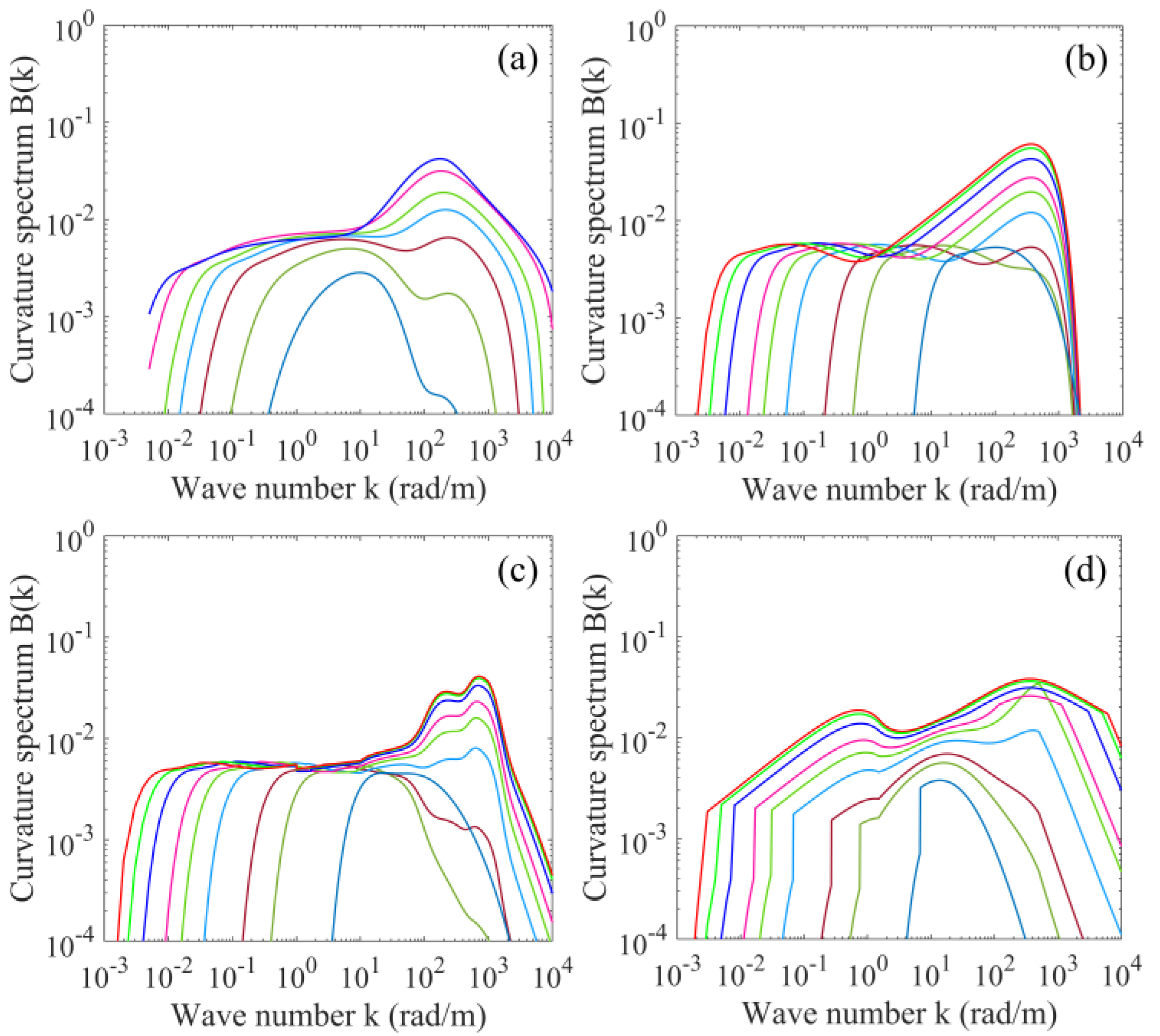
The PO, GO, and GO4 are known to be three of the most commonly used models to represent the microwave backscatter from ocean surface at low incidence angles. The surface is assumed to be Gaussian considering that the effects of non-Gaussianity are small and are often neglected at low incidence angles [11]. At small incidence angles (less than 20° approximately), the reference model for ocean radar backscatter is the PO model, which is derived from the Stratton-Chu integral equations with the high-frequency Kirchhoff approximation. For a Gaussian ocean surface, the monostatic NRCS according to the PO approximation takes the form of the so-called Kirchhoff integral:

$${\sigma }_{\mathrm{PO}}^0=\frac{K^2}{\pi {\cos }^2\theta }{\left|R\right|}^2{\displaystyle \int \exp \left(-i2{\mathit{K}}_{\mathit{h}}·\mathit{r}\right)\exp \left(-4K_z^2({\sigma }^2-\rho (\mathit{r}))\right)}d\mathit{r}$$

(1)

where R is the Fresnel reflection coefficient at normal incidence on a flat water surface, θ is the incidence angle, K is the wave number magnitude, K_h and K_z are the horizontal and vertical components of the incident wave vector, r is the horizontal space vector, σ² is the sea surface mean square height, and ρ is the autocorrelation function. σ² and ρ are related to the ocean wave number spectrum F by:

$${\sigma }^2={\displaystyle {\int }_{-\infty }^{\infty }F(\mathit{k})d\mathit{k}}$$

(2)

$$\rho \left(\mathit{r}\right)={\displaystyle {\int }_{-\infty }^{\infty }F\left(\mathit{k}\right)\exp \left(i\mathit{k}·\mathit{r}\right)d\mathit{k}}$$

(3)

where k is the ocean wave vector. For very large Rayleigh parameters (4K²cos²θσ²→∞), the PO reduces to the GO approximation. In the limit of an isotropic Gaussian surface, the GO model is given by:

$${\sigma }_{\mathrm{GO}}^0=\frac{{\left|R\right|}^2}{\mathrm{mss}}{\sec }^4\theta \exp \left(-\frac{{\tan }^2\theta }{\mathrm{mss}}\right)$$

(4)

where mss represents the sea surface mean square slope. This simple model is derived with some assumptions that are clearly violated under realistic ocean conditions. It neglects the diffraction induced by the roughness scales much shorter than the radar wavelength. Thus, it deviates from the actual NRCS in the microwave regime. To improve the model, a “radar-filtered” mss should be adopted to compensate for the missing diffraction term artificially:

$${\mathrm{mss}}_f={\displaystyle {\int }_0^{k_c}{k}^{2}F(\mathit{k})d\mathit{k}}$$

(5)

where k_c is the high-limit cutoff wave number for waves that contribute to the filtered mss. In addition, the diffractive processes of the small-scale roughness can modify the reflection properties of a real ocean surface. Thus, for the GO model, an effective reflection coefficient should be adopted [33]:

$${\left|R_{\mathrm{eff}}\right|}^2=a\times {\left|R\right|}^2\left[1-\left(4K^2{\sigma }_s^2\left(k_d\right)\right)\right]$$

(6)

where R_eff is the nadir effective reflection coefficient, a accounts for the long-wave tilting effect, ${\sigma }_s^2$ is the mean square height of small-scale waves, k_d is the low-limit cutoff wave number for shortwaves that diffract the incident radar pulse and affect the surface reflection process.

The GO4 is an improved version of GO with the introduction of a diffraction correction quantified by an effective msc. In the isotropic case, it is given by:

$${\sigma }_{\mathrm{GO}4}^0={\sigma }_{\mathrm{GO}}^0\left(1+\frac{{\mathrm{msc}}_e}{16K^2{\mathrm{mss}}^2{\cos }^2\theta }\left[\frac{{\tan }^4\theta }{{\mathrm{mss}}^2}-4\frac{{\tan }^2\theta }{\mathrm{mss}}+2\right]\right)$$

(7)

where mss is assumed to be the total mss (for the total mss, k_c→∞), msc_e is the effective mean square curvature:

$${\mathrm{msc}}_e={\displaystyle {\int }_0^{k_r}{k}^{4}F(\mathit{k})d\mathit{k}}$$

(8)

where k_r is the high-limit cutoff wave number for waves that have meaningful curvature.

2.3. Wave Spectrum

As seen in Section 2.2, some statistical parameters of the ocean surface such as auto-correlation function, mean square height, mean square slope, and mean square curvature are needed to evaluate the PO, GO, and GO4 models, and these quantities can be obtained from forms of the full ocean wind wave spectrum that have been developed by various workers. In this paper, four wave spectral models denoted as D (Donelan-Banner-Plant), E (Elfouhaily et al.), K (Kudryavtsev et al.), and H (Hwang et al.) are considered. The details of the D spectrum are available in [34]. Of particular note is that a variable wind speed should be used in the spectral computation for producing reasonable NRCS values at low winds; a standard deviation of 1.5 m/s is suggested [35]. The E spectral model is described in [36], and has been widely used in ocean radar sensing. The K spectral model is first described in [37], then it is improved in [20,38] (see Appendix A of [38] for the detailed description of the last version of the K spectrum). The numerical code obtained from M. Yurovskaya (personal communication, 2019) is used for simulations. The H spectrum is proposed in [39] and then refined several times [40,41,42]. The version of the spectral model with the corrections made in [42] is adopted.

Figure 1 illustrates the D, E, K, and H azimuthally integrated curvature spectra B(k) for wind speeds of 1, 3, 5, 10, 15, 20, 30, 40, and 50 m/s in log-log scales. It can be seen that there are some similarities in the spectral distributions of the ocean surface roughness between the four models. All spectra suggest that the dominant contribution of surface mss comes from intermediate- and short-scale waves roughly from 1 to 1000 rad/m; there is a spectral peak near 300 rad/m, followed by a rapid dropoff in the capillary wave region; the wind speed sensitivity of the spectral density of surface waves decreases with the wind speed increasing, and furthermore the spectral density of decimeter- to meter-scale waves is much less sensitive to wind speed. This may be partially explained by the fact that waves of these scales are the dominant regions of wave breaking for generating short-scale waves [43].

Even more remarkably, the four spectral models are different from each other in many ways. Each is developed to correspond to a given set of experimental data and solve a specific problem. The D spectrum is the synthesis of the results of measurements with wave gauge arrays, stereo photography, and microwave backscatter carried out at wind speeds roughly from 5 to 25 m/s. Thus, its validity at extremely low and high winds is rather questionable. The D spectrum becomes less and less available at extremely high wind speeds for the presence of more and more outliers, as seen in Figure 1a. The E spectrum is based on the unification of optical, in situ, and tank data. It emphasizes the consistency with the measured mss in [9]. The wind speed in the data set ranges approximately from 2 to 17 m/s. The K spectrum is derived considering the energy balance equation under the joint action of wind forcing, viscous dissipation, wave-wave interactions, dissipation via wave breaking, and generation of parasitic capillaries by wave breaking, with the constraints provided by field stereo photograph data observed at wind speeds from 4 to 17 m/s. The H spectrum is a parameterized roughness spectrum derived from the field measurements obtained from free-drifting wave gauges at wind speeds of 2.4–14 m/s. Additionally, the H spectrum is modified for wind speeds of 15–50 m/s based on the Ku2001 geophysical model function (GMF) [44], C-band GMF (CMOD5, [45]), and L-band GMF [46,47].

3. Results

The PO, GO, and GO4 are three popular quasi-specular models built with different degrees of approximation and in the absence of wave breaking. They will certainly show different performances in describing the low-incidence microwave backscatter from the ocean surface at different incidence angles under different wind conditions. Particularly, the models may be limited in their abilities to characterize the surface radar backscatter at high winds where wave breaking effects will probably become non-negligible. In this section, the abilities of the PO, GO, and GO4 models to reproduce the Ku-band NRCS at incidence angles of 0–18° over the wind speed range of 0–45 m/s are systematically compared and analyzed by comparing their predictions to the radar measurements. On this basis, the limitations of the quasi-specular scattering theory and the effects of wave breaking are discussed to further expound the Ku-band ocean radar backscattering mechanism at low incidence angles at high winds.

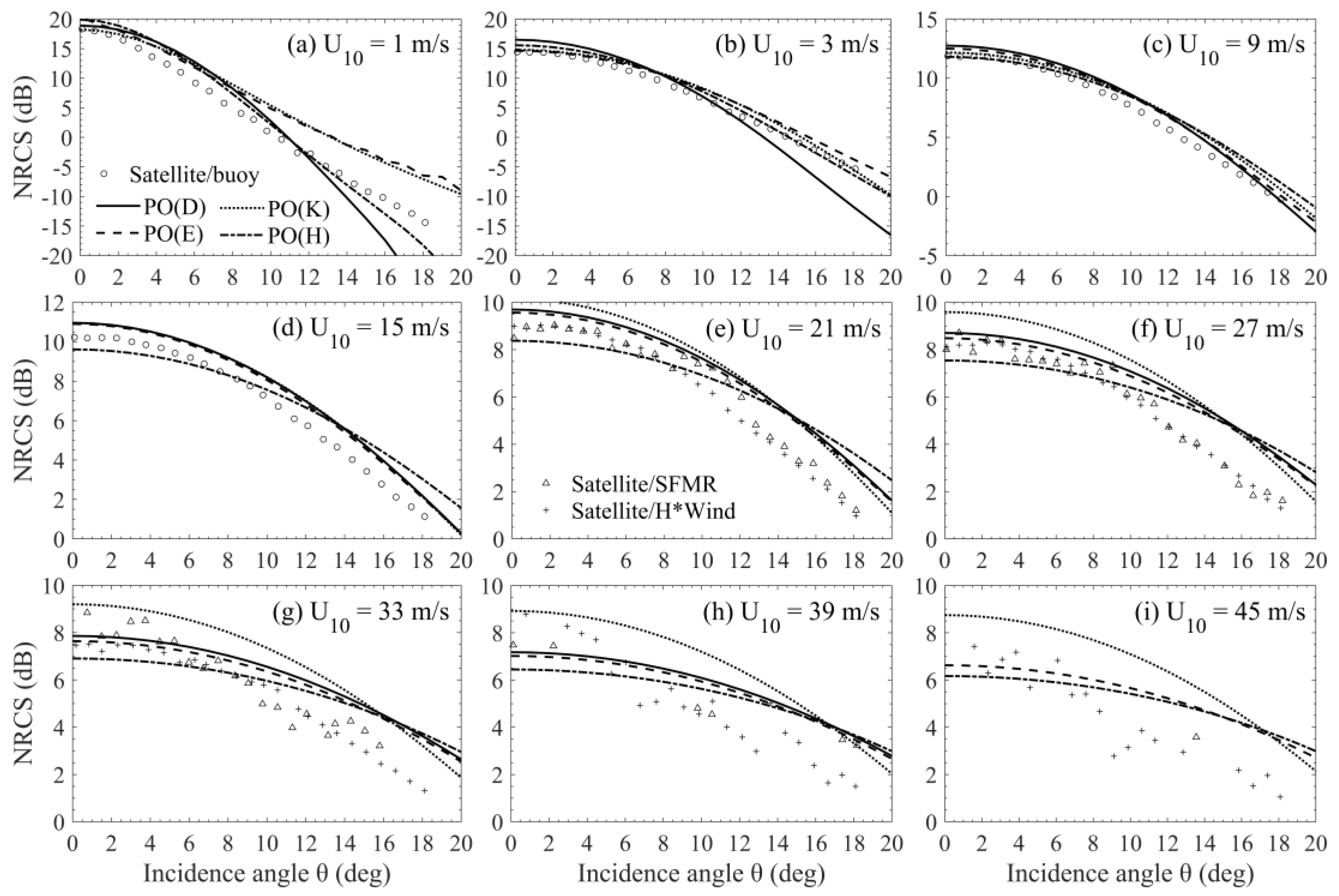
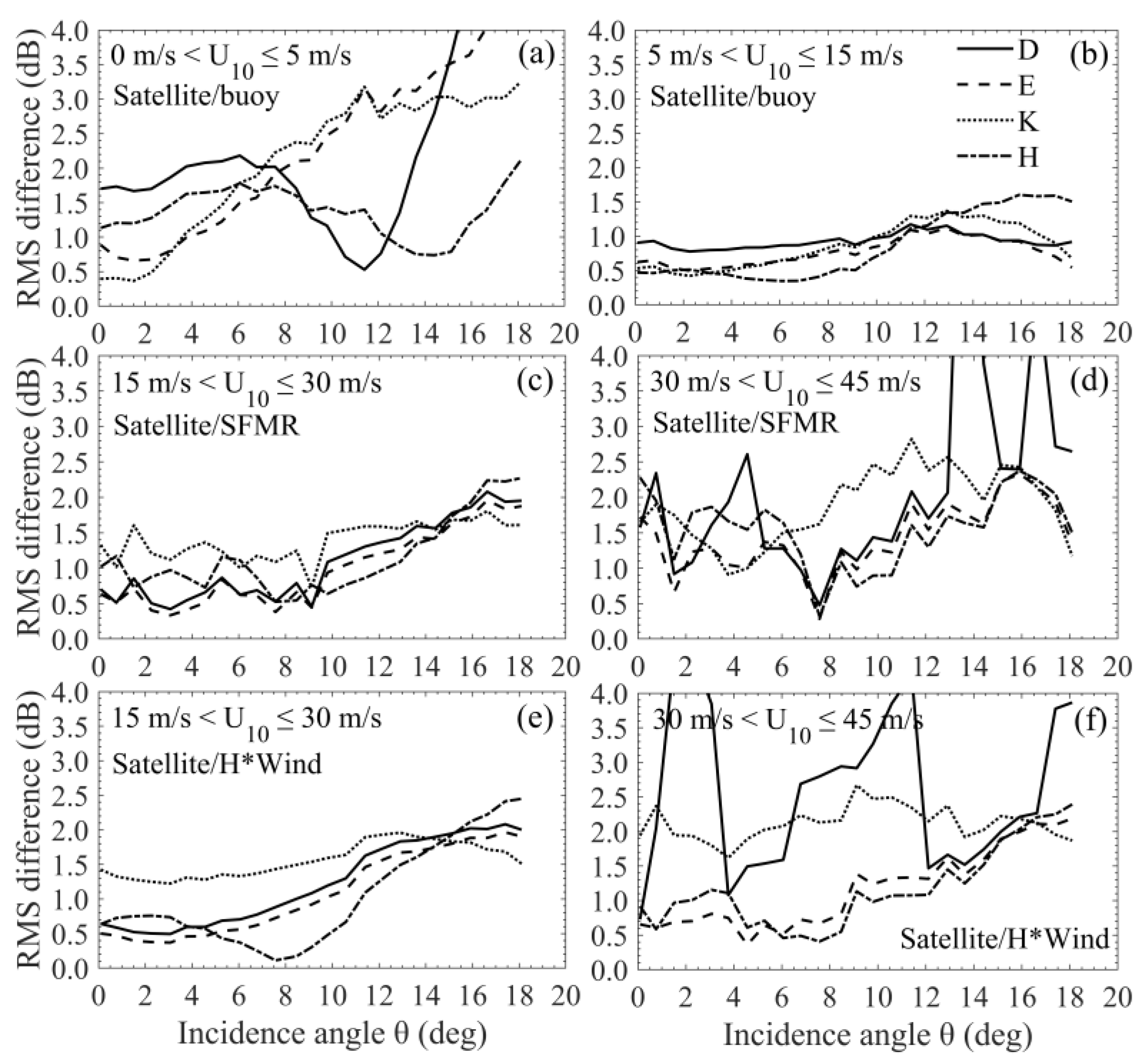
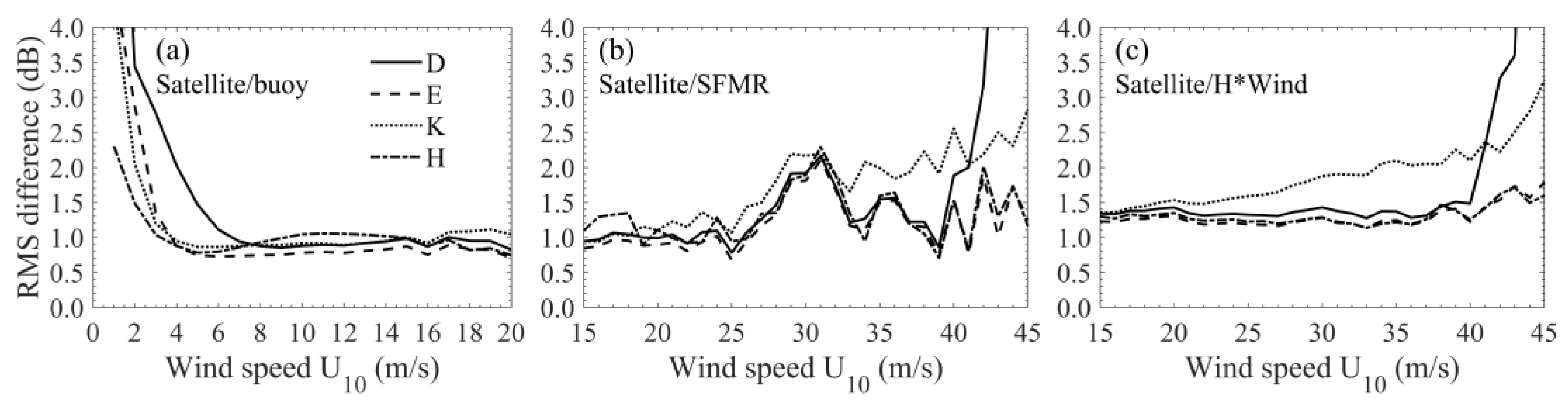
3.1. Comparison of the PO Model with Measurements

The omnidirectional backscattering predictions of the PO model with D, E, K, and H spectra input are compared with the satellite NRCS measurements, along with simultaneous wind truth from buoy, SFMR, and H*Wind data, for wind speeds up to 45 m/s. The radar wave number magnitude K is about 289 rad/m for TRMM and 285 rad/m for GPM. The small difference has very little influence on the results, and K is set to 289 rad/m in this paper. The satellite/buoy data are used as reference at low to moderate winds, and at higher winds are the satellite/SFMR and satellite/H*Wind data. The NRCS measurements are binned into specified wind speed intervals at each PR (or KuPR) incidence angle. The wind speed bin width is set to 1 m/s. The 25 different incidence angles are from 0.1 to 18.1°, and the bin width is set to 0.2°. The differences between the PO model computations using D, E, K, and H spectra and the mean σ⁰ in each wind speed and incidence angle 2-D bin are calculated in dB. Then, the root mean square (RMS) of the differences at selected wind conditions at each incidence angle RMS(θ) and the RMS of the differences at all incidence angles at each wind speed RMS(U₁₀) defined as:

$$\mathrm{RMS}\left(\theta \right)=\sqrt{\frac{{\displaystyle {\sum }_{i=1}^M{\left({\sigma }_{\mathrm{PO}}^{0\mathrm{d}B}\left(U_{10}{}_i,\theta \right)-{\sigma }_{\mathrm{meas}}^{0\mathrm{d}B}\left(U_{10}{}_i,\theta \right)\right)}^2}}{M}}$$

(9)

$$\mathrm{RMS}\left(U_{10}\right)=\sqrt{\frac{{\displaystyle {\sum }_{i=1}^N{\left({\sigma }_{\mathrm{PO}}^{0\mathrm{dB}}\left(U_{10},{\theta }_i\right)-{\sigma }_{\mathrm{meas}}^{0\mathrm{dB}}\left(U_{10},{\theta }_i\right)\right)}^2}}{N}}$$

(10)

can be obtained, where ${\sigma }_{\mathrm{PO}}^{0\mathrm{dB}}$ is the PO-simulated σ⁰ in dB, ${\sigma }_{\mathrm{meas}}^{0\mathrm{dB}}$ is the measured σ⁰ in dB, M is the number of wind speed bins at selected wind conditions, and N is the number of incidence angle bins. Figure 2 displays examples of comparison between the PO model computations using D, E, K, and H spectra and the mean values of binned NRCS measurements as functions of incidence angle at weak to severe winds. The RMS differences as functions of incidence angle at different wind conditions are shown in Figure 3. Figure 4 shows the RMS differences at all incidence angles as functions of wind speed.

As seen in Figure 2a,b, Figure 3a and Figure 4a, the PO-simulated NRCSs deviate from the measurements, particularly at incidence angles near 18°, and the deviations increase rapidly with the decrease of wind speed at low winds (0–5 m/s) where the PO model containing quasi-specular and diffuse diffraction contributions should be adequate considering that wave breaking hardly occurs. The large deviations probably result from the imperfections of the wind-wave spectra, which refer to the fact that the spectra have limited validity due to the lack of experimental data at extremely low winds, and more importantly, they do not cover the swell portion, but which is recognized to have a particularly significant impact on the radar backscatter at low winds [48]. As will be seen in Section 4.1, the impact of swell is indeed significant at low winds. Moreover, it is more serious near 18° than near nadir. The great uncertainties of the NRCS measurements and wind truth at low winds also make important contributions to the large deviations [49]. In addition, the non-Gaussian effects come into play at larger incidence angles. However, it has been indicated in [13] that the non-Gaussian correction has little impact on the performance of the PO model with the E spectrum input in predicting the omnidirectional NRCS at small winds. Figure 4a shows at low winds that the D spectrum yields larger RMS deviations with a larger inflection point (about 6 and 4 m/s for the other spectra), i.e., the D spectrum generally performs the worst as the corresponding experimental data are badly lacking low wind cases.

From Figure 2c,d, Figure 3b and Figure 4a, it is found that the PO model is rather accurate at moderate winds (5–15 m/s). Figure 3b shows that the RMS deviations remain within 1 dB in the first 10° of incidence, then become slightly larger (but not more than 1.5 dB) at higher incidence probably due to the neglect of non-Gaussian effects. It has been found in [13] that this neglect can result in overestimation of the PO model, and the overestimation increases with the incidence angle. However, for the D, E, and K spectra, the overestimation anomalously decreases with the incidence angle in 13–18° where the RMS deviations exhibit a slightly decreasing trend. This might be because the PO model with D, E, and K spectra input undervalues the Bragg scattering contribution increasingly with the incidence angle. Figure 4a shows that the RMS deviations remain around 1 dB over the moderate wind speed range.

At high wind speeds of 15–30 m/s, the PO model exhibits relatively small differences with the radar measurements at lower incidence angles where the D, E, and K spectra yield slightly higher NRCS and the H spectrum yields slightly lower NRCS, while at larger incidence angles, the PO model shows a significant overestimation that somewhat increases with wind speed for all the four spectra (Figure 2e,f). With the satellite/SFMR data used as reference, RMS(θ) remains mostly within 0.5–1 dB for the D, E, and H spectra and 1–1.5 dB for the K spectrum at incidence angles less than about 10°, then shows an increasing trend at higher incidence, and finally reaches about 2 dB for D and E, 1.6 dB for K, and 2.3 dB for H (Figure 3c); RMS(U₁₀) remains around 1 dB at first, but exhibits an abnormal spike around 30 m/s perhaps owing to the uncertainties in the SFMR wind speed (Figure 4b). With the satellite/H*Wind data used as reference, RMS(θ) generally increases with incidence angle and reaches a value within 1.5–2.5 dB at 18.1° (Figure 3e); RMS(U₁₀) remains around 1.3 dB for the D, E, and H spectra and increases from about 1.3 to 2 dB for the K spectrum at wind speeds of 15–30 m/s (Figure 4c).

As shown in Figure 3b–e, the RMS derivations are larger at high winds than at moderate winds at higher incidence angles (e.g., >10–12°) where the PO model overestimates the NRCS and the overestimation somewhat increases with wind speed. Figure 5 displays the differences between the omnidirectional PO computations (dB) using D, E, K, and H spectra and the azimuthally averaged NRCS (dB) obtained with the Ku-band NSCAT4 HH GMF as functions of wind speed at incidence angle of 18°. NSCAT4 GMF [50] is given as lookup tables of ${\sigma }_{pp}^0\left(\theta ,U_{10},\phi \right)$, where θ is the incidence angle in the range of 16–66° in 1° intervals, U₁₀ wind speed from 0.2 to 50 m/s in 0.2 m/s intervals, φ the azimuthal angle from 0 to 180° in 2.5° intervals, and pp polarization. The HH GMF is selected to keep in line with the radar measurements. Figure 5 again indicates that the PO model overestimates the NRCS more significantly at high winds than at moderate winds at an incidence angle of 18°. The larger overestimation should not be ascribed to the assumption of non-polarization of the PO model as NSCAT4 indicates the polarization ratio at 18° is about 0.2 dB at moderate winds and 0.1 dB at high winds. The overestimation resulting from the neglect of non-Gaussian effects increases with wind speed but merely at wind speeds lower than about 10 m/s [13]. It shows a decreasing trend at higher winds [13] where the PO model still has an increasing overestimation. The feasible explanation for this should be that the wave breaking, which is more and more dramatic with wind speed increasing, produces sea foam, spray, and bubbles, which can make the ocean surface more “smooth” and thus make the NRCS near 18° smaller. The overestimation tends to be stable with wind speed increasing.

As wind speed continues to increase and exceeds 30 m/s, the PO model becomes less and less available; it becomes completely unavailable with wind speed exceeding a threshold value between 33 and 39 m/s (Figure 2g–i). Figure 6 displays the comparison between the PO model computations with E spectrum input and the bin-averaged NRCS measurements from the satellite/H*Wind data at wind speeds of 34–38 m/s in 1 m/s intervals. It can be seen that the PO model fails completely when wind speed exceeds about 37 m/s where it cannot describe the linear dependence of the low-incidence NRCS on the incidence angle, implying that the wave breaking effects instead of the quasi-specular scattering have become dominant. Figure 3d,f and Figure 4b,c indicate that, at severe winds, the performance of E and H spectra is relatively good; the K spectrum yields larger RMS deviations that increase slowly with wind speed; for the D spectrum, the RMS deviations remain relatively small until wind speed reaches about 40 m/s, followed by a rapidly increasing trend as this spectrum becomes less and less available.

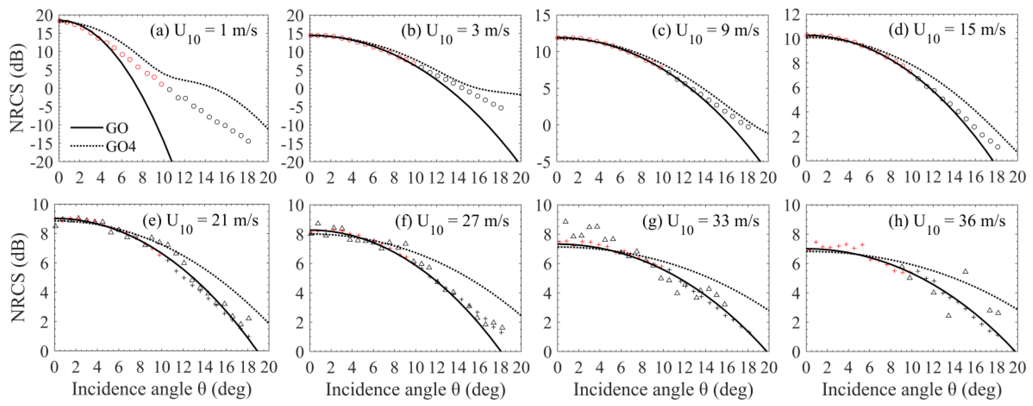
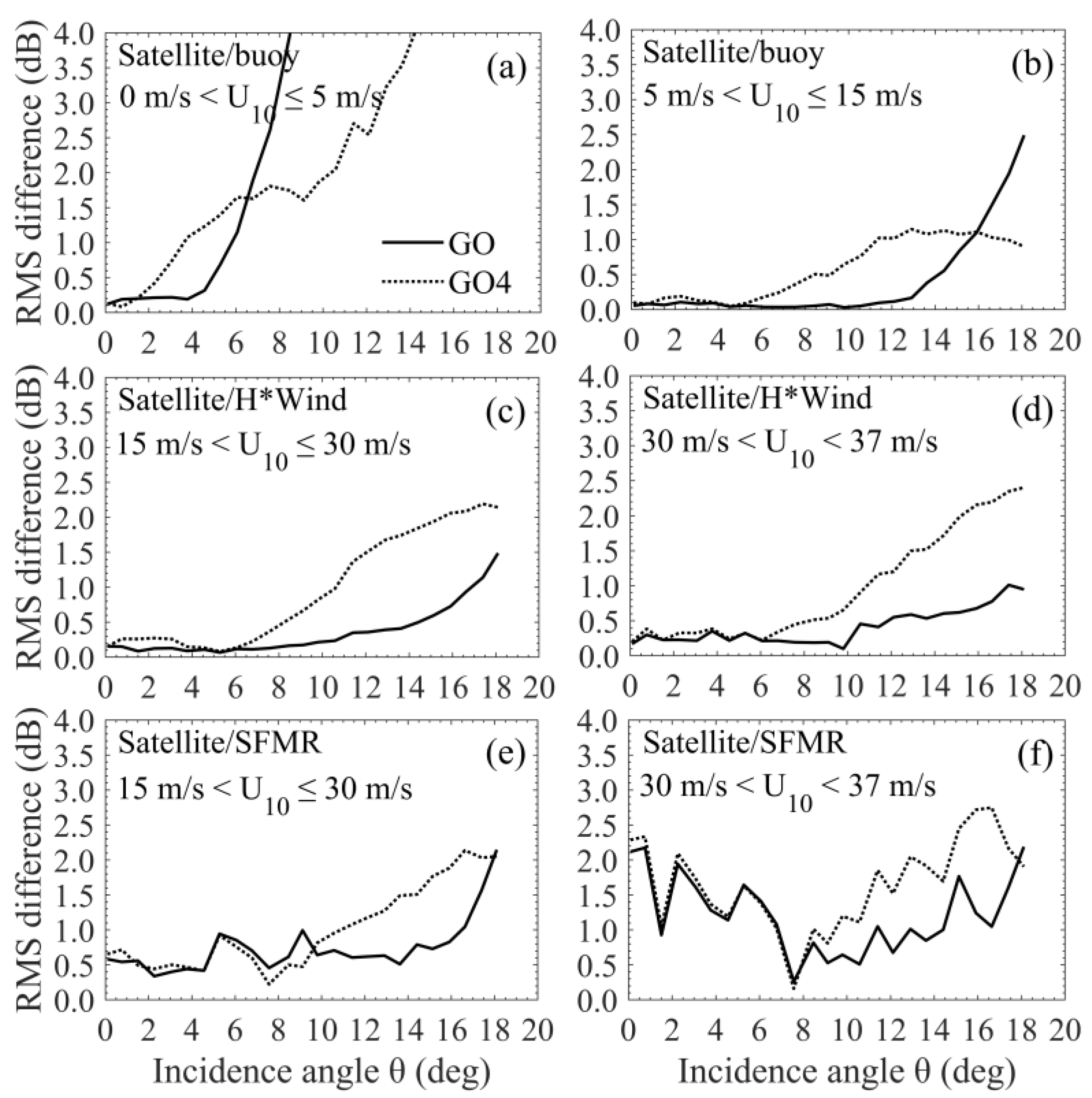
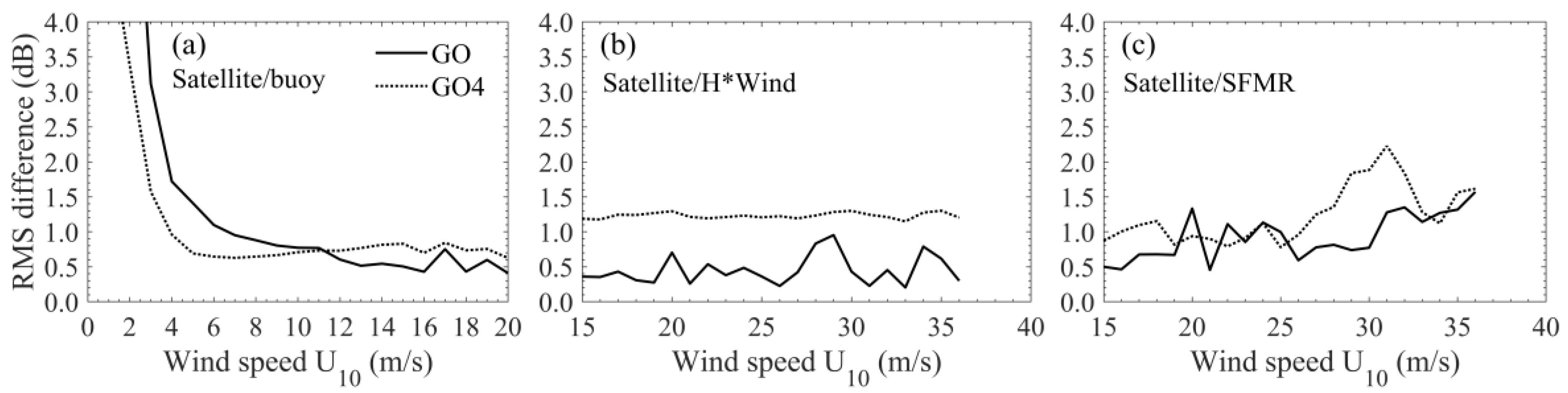
3.2. Comparison with GO and GO4 Models

For practical applications, it is useful to have a simple scattering model at hand, which relates the quasi-specular NRCS at low incidence angles to just a limited number of parameters instead of the roughness spectrum. To reach this aim, the GO model and its improvement GO4 are tested for the omnidirectional NRCS at wind speeds less than 37 m/s. The GO model is parameterized by the effective reflectivity and filtered mss parameters. In the GO4 model, the total mss and the effective msc are the two key parameters. Here, the values of these parameters are directly estimated from the nonlinear least squares fits of (4) or (7) to the collocated datasets without any a priori knowledge of the ocean surface. The fits are done in linear units. In the fitting process, the satellite/buoy data are used as reference at lower wind speeds, and at higher wind speeds (>15 m/s) are the satellite/H*Wind data. The wind speed bin width is set to 0.2 m/s. In addition, the fits are restricted to 0° ≤ θ ≤ 10° where the NRCS is dominantly contributed by the quasi-specular reflection over the wind speed range of 0–37 m/s. The contribution from resonant Bragg scattering increases at larger incidence angles.

Figure 7 illustrates the fits of the GO and GO4 models and their comparison with the bin-averaged NRCS measurements at selected wind speeds. Figure 8 shows the RMS of differences between the model predictions and the bin-averaged NRCS measurements at different wind conditions as a function of incidence angle. Figure 9 shows the RMS of differences at all incidence angles as functions of wind speed. As can be seen, the GO model achieves reasonably good agreement at lower incidence angles where the RMS deviations with respect to the satellite/buoy and satellite/H*Wind data remain at a rather low level of about 0.1–0.3 dB due to the direct determination of the model parameters by fitting these data. At higher incidence angles, the GO model underestimates the NRCS, and the underestimation increases with incidence angle. The model ignores the curvature effects. The use of a filtered mss can only partially compensate for the missing diffuse diffraction term, which accounts for the contributions from roughness scales comparable to or shorter than the radar wavelength. In particular, the contribution from resonant Bragg scattering, which becomes increasingly significant with incidence angle, is not incorporated at all [7]. Moreover, the underestimation somewhat decreases with wind speed, and it becomes pretty small at high to severe winds. This is probably because the fraction of Bragg scattering contribution decreases with wind speed [34], and the increase of NRCS caused by Bragg scattering can be offset by the decrease of NRCS caused by wave breaking.

At low winds (U₁₀ ≤ 5 m/s), the NRCS underestimation of the GO model at higher incidence angles is relatively significant (Figure 7a,b). The RMS deviations exhibit a very rapid increasing trend at incidence angles higher than about 4° (Figure 8a). They also increase rapidly with the decrease of wind speed (Figure 9a). The abnormally large underestimation at extremely low winds might be mainly because the Rayleigh parameter is not big enough for the GO asymptotic method [15]. The limited validity can be improved by introducing a non-Gaussian shape for the scattering diagram or an incidence-dependent cutoff in the definition of the filtered mss [51]. At higher winds (5 m/s < U₁₀ < 37 m/s), the GO model is found rather accurate over almost the whole range of incidence angles (Figure 7c–h). The RMS deviations with respect to the satellite/buoy and satellite/H*Wind data remain within 0.1–0.3 dB at lower incidence angles (e.g., <10°), then show a slightly increasing trend at higher incidence angles (Figure 8b–d). They remain within 1 dB at wind speeds larger than about 8 m/s (Figure 9a,b). The RMS deviations with respect to the satellite/SFMR data behave similarly though with slightly larger values except that there is an abnormal spike near nadir at extremely high winds (as shown in Figure 8f), which has the same cause with the abnormal spike shown in Figure 4b.

As seen in Figure 7, the GO4 model yields good agreement with the measurements at lower incidence angles. Then, it overestimates the NRCS at higher incidence angles probably due to the introduction of a diffraction term involving the curvature of the ocean surface. At low winds, the GO4 model gradually deviates from the radar measurements with the incidence angle increasing, and exhibits a rather large overestimation near 18° at extremely low winds where the sea surface roughness might be too small to satisfy the large Rayleigh parameter assumption required by the GO4 asymptotic theory (Figure 7a,b). Figure 8a and Figure 9a show respectively that the RMS deviations increase rapidly with the increase of incidence angle and with the decrease of wind speed at low winds. At higher winds, the GO4 model achieves good performance at lower incidence angles and overestimates the NRCS at higher incidence angles (Figure 7c–h). The RMS deviations remain relatively low at incidence angles less than about 6°, then show an increasing trend at higher incidence angles (Figure 8b–f). Figure 8f shows a spike near nadir for the GO4 model as well. Similar to the PO model, the overestimation of the GO4 model decreases with the incidence angle in 13–18° at moderate winds (Figure 8b), and somewhat increases with speed at moderate to high winds (Figure 7c–f).

As seen in Figure 7 and Figure 8, the GO model yields better agreement with the radar measurements than the GO4 model at lower incidence angles at low to moderate winds and over almost the whole range of incidence angles at high to severe winds. From Figure 2 and Figure 7, it can be found that the GO4 model can achieve the same order of magnitude as the PO model, and it behaves very similar to the PO model with E spectrum input. Figure 3 and Figure 8 show that the GO4 model generally brings an improvement over the PO model at incidence angles less than about 12°. The reason for this might be that the GO4 model parameters are directly estimated from the measurements and do not require an assumed knowledge of the ocean wave spectrum whose estimation can suffer from great uncertainties. In addition, the GO4 model can absorb non-Gaussian effects by the msc parameter, which may not be neglected for the low-incidence scattering diagram and cannot be easily rendered with the PO model [7,15].

For the GO model, the Fresnel reflection coefficient, which is a function of incidence angle and dielectric constant (see, e.g., [52]), is just applicable for effective smooth surfaces without any roughness scales comparable to or smaller than the radar wavelength. Its dependence on the incidence angle is very weak, and it should not vary with wind speed [11]. For rough sea surfaces, a wind speed dependent nadir effective reflection coefficient should be adopted. Here, the nadir effective reflectivity |R_eff|² is estimated jointly with the filtered mss at each wind speed from the least squares fit of the GO model to the radar measurements across incidence angles less than 10°. Figure 10a shows the solutions for |R_eff|² versus wind speed (crosses). As seen, |R_eff|² varies roughly between 0.27 and 0.48, and has a mean value of 0.39 in the wind speed range of 0–37 m/s. The |R_eff|² estimates are slightly smaller than the corresponding ones given in Figure 6 of [11], perhaps due to the differences among the reference datasets. At wind speeds greater than about 6 m/s, |R_eff|² decreases with the wind speed increasing. This is true because the small-scale ocean surface roughness diffracts the incident electromagnetic wave, which reduces the effective reflectivity by a factor of $1-4K^2{\sigma }_s^2$, where ${\sigma }_s^2$ is the mean square height of the small-scale waves. The |R_eff|² rapid increasing trend at lower winds might be the combined effect of the short-waves diffraction and the long-waves tilt that affects the backscatter by modifying the local incidence angle. The sum of a linear and a logarithmic function as:

$$f\left(U_{10}\right)=A_1+A_2{U}_{10}+A_3{\log }_{10}\left(U_{10}\right)$$

(11)

can be used to parameterize the |R_eff|², where U₁₀ is the 10-m wind speed, A₁, A₂, and A₃ are constants to be determined empirically. Figure 10a shows an optimal parameterization based on a least square fitting of the data points at 0 < U₁₀ < 37 m/s (black line). It is conducted in two wind speed ranges. The coefficients A₁ = 0.2315, A₂ = 0.0707, and A₃ = −0.0141 at wind speeds less than 3.5 m/s. At higher wind speeds, they are 0.4535, −0.0090, and 0.0893, respectively. Figure 10b shows the parameterization accuracy. It can be seen that the normalized deviations, which denotes the parameterized values divided by the values inferred from the radar measurements minus one, are mainly within about 10%.

As shown by (6), |R_eff|² is physically related to a coefficient a that accounts for the tilting effect of long waves and a low-limit cutoff wave number k_d, above which roughness diffracts the radar wave and affects the ocean surface reflection process. Coefficient a should be less than or equal to 1, and k_d might vary with wind speed. For simplicity, a is set to 1 here and the tilting effect is incorporated in k_d. Given a wave spectral model, it is straightforward to integrate the wave spectrum at each wind speed to determine the required cutoff wavenumber k_d based on the accurate estimates of |R_eff|² from radar measurements. Figure 10c shows the estimates of ratio of k_d to radar wave number K for the D, E, K, and H spectra. For every spectrum, k_d shows an increasing trend with wind speed increasing up to about 15 m/s, followed by a saturation for higher winds. The k_d estimates are basically a tenth to three fifths of K in the wind speed range of 0–37 m/s. The k_d calculated with the K spectrum has the smallest change interval, then is the E spectrum, and the intervals for the D and H spectra are slightly wider. All the four spectra can yield excellent agreement with the |R_eff|² estimated from radar measurements.

Figure 10d shows the estimates of the filtered mss (mss_f) from the radar measurements with the GO model (crosses). As can be seen, mss_f is roughly a nonlinear monotonically increasing function of wind speed, and the magnitude increases approximately from 0.004 to 0.06 with wind speed ranging from 0 to 37 m/s. It can be accurately parameterized by (10) in three wind speed ranges, see the black line in Figure 10d. For wind speeds below 3.5 m/s, A₁ = −0.0019, A₂ = 0.0066, and A₃ = −0.0056; for wind speeds above 10 m/s, A₁ = −0.0140, A₂ = 0, and A₃ = 0.0453; in the middle, A₁ = 0.0034, A₂ = −0.0002, and A₃ = 0.0296. Figure 10e shows the normalized deviations of the parameterization, which are larger at extremely low winds and at higher winds but mostly within 15%. The wind speed dependence of mss_f is in rather good agreement with the result shown in Figure 7 of [11] in the wind speed range of 1–25 m/s.

Given a wave spectral model, mss_f can be obtained by integrating the slope spectrum from zero to an upper bound cutoff wave number k_c. In light of the past studies, k_c is usually a sixth to third of the radar wave number K (e.g., [53]). Figure 10d shows the mss_f values integrated over the wave number range of 0 to k_c = K/5 for the D, E, K, and H spectra. Compared with the mss_f estimated with the GO model, when k_c = K/5, the H spectrum yields the best agreement at low winds (<5 m/s), but the most significantly increasing overestimation at higher wind speeds. The D spectrum undervalues slightly the lower winds (about < 8 m/s) but overestimates the higher winds. The E spectrum overvalues the low winds, followed by a slight underestimation at moderate to high winds, and again becomes overvalued at even higher winds. The K spectrum yields an overestimation at wind speeds < about 20 m/s and a slight underestimation at higher winds. The D and E spectra seem to provide an overall better agreement at moderate winds (5–15 m/s). At higher winds, the K spectrum yields the best agreement. All in all, the mss_f obtained from the GO model is indeed on the level of the radar filtered mss.

The required k_c should vary with wind speed, and its values for the D, E, K, and H spectra at each wind speed are determined through minimizing the difference between the integrated mss_f and the mss_f estimated with the GO model. Figure 10f shows the estimates of ratio of k_c to K as a function of wind speed. As shown, the H spectrum becomes unsuitable for the k_c estimation when wind speed exceeds about 30 m/s where the k_c values are too small to be within the assumed widest reasonable range of K/1.5–K/40 (e.g., [53]). The D spectrum fails at low winds with too large k_c values. By contrast, the k_c values obtained with the E and K spectra are reasonable (mostly within K/20–2K/5) over the whole wind speed range of 0–37 m/s. The two spectra can yield good agreement with the mss_f from GO.

For the GO4 model, the total mss (mss_t) and the effective msc (msc_e) come into play to avoid the use of the filtered mss. The mss_t is an intrinsic parameter of the ocean surface and does not depend on the radar frequency. Instead, the frequency dependence is rendered by the msc_e, a curvature parameter to quantify the diffraction correction. Figure 11a shows the mss_t values obtained from a joint estimation of mss_t and msc_e with a least squares fit of the GO4 model to the radar measurements at each wind speed (crosses). The first 10° of the scattering diagram, which is assumed to be the minimal domain of validity of the GO4 model, is used for the fits. The mss_t exhibits a monotonically increasing trend similar to mss_f, but with larger magnitudes ranging roughly from 0.01 to 0.16 over the wind speed range of 0 to 37 m/s. It can also be parameterized by (10) in two wind speed ranges, as shown by the black line in Figure 11a. The coefficients A₁, A₂, and A₃ are 0.0055, 0.0107, −0.0095 at lower winds (<3.5 m/s), 0.0251, 0.0041, −0.0037 at higher winds. As seen in Figure 11b, the accuracy of the parameterization is mostly within 5% compared to the best-fit solutions of mss_t based on the radar data.

For comparison, Figure 11a displays the total mean square slopes from the clean water sun glitter data reported by Cox and Munk in [9] (squares) and those calculated with the D (dark red line), E (olive green line), K (dodger blue line), and H (deep pink line) spectra using the frequency cutoff at 2000 rad/m. As expected, the mss_t estimated with the GO4 model is indeed of the same order of magnitude as the total mss. The mss_t estimated with GO4 is slightly larger than the total CM54-mss (short for the data of Cox and Munk) and the integrated mss_t at wind speeds lower than about 10 m/s. It exhibits good agreement with the CM54-mss in the wind speed range of 10–15 m/s. At wind speeds of 10–20 m/s, the E spectrum yields relatively good agreement, and at higher winds is the D spectrum. The results at moderate wind speeds (5–15 m/s) are mostly consistent with those shown in Figure 9 of [7].

Figure 11c shows the estimates of msc_e with the GO4 model (crosses) and the corresponding best-fit two-branch parameterization (black line). The msc_e can be accurately parameterized by (10) in two wind speed ranges with normalized deviations mostly within 10% (Figure 11d). The coefficients A₁ = −28.2956, A₂ = 132.2182, and A₃ = −86.9817 at wind speeds lower than 6 m/s, and A₁ = 1633.2296, A₂ = 240.8675, and A₃ = −3077.4938 at higher winds. As seen in Figure 11c, the msc_e estimated with the GO4 model increases from 100 to 6000 with wind speed increasing from 1 to 37 m/s, which is at the same order of magnitude with that shown in Figure 10 of [7]. The msc_e can also be obtained by cumulating the spectral curvature with a high-limit cutoff wave number k_r. Based on the estimated msc_e with the GO4 model, the estimates of ratio of k_r to K are determined for the D, E, K, and H spectra and plotted versus wind speed in Figure 11e. As shown, the k_r values are too large at low wind speeds for the D, K, and H spectra. In contrast, the k_r estimated with the E spectrum is reasonably within 1 to 2 times of K, which is consistent with the results given in [7]. In other words, only the E spectrum can achieve good agreement with the msc_e obtained from the GO4 model over the whole wind speed range of 0–37 m/s.

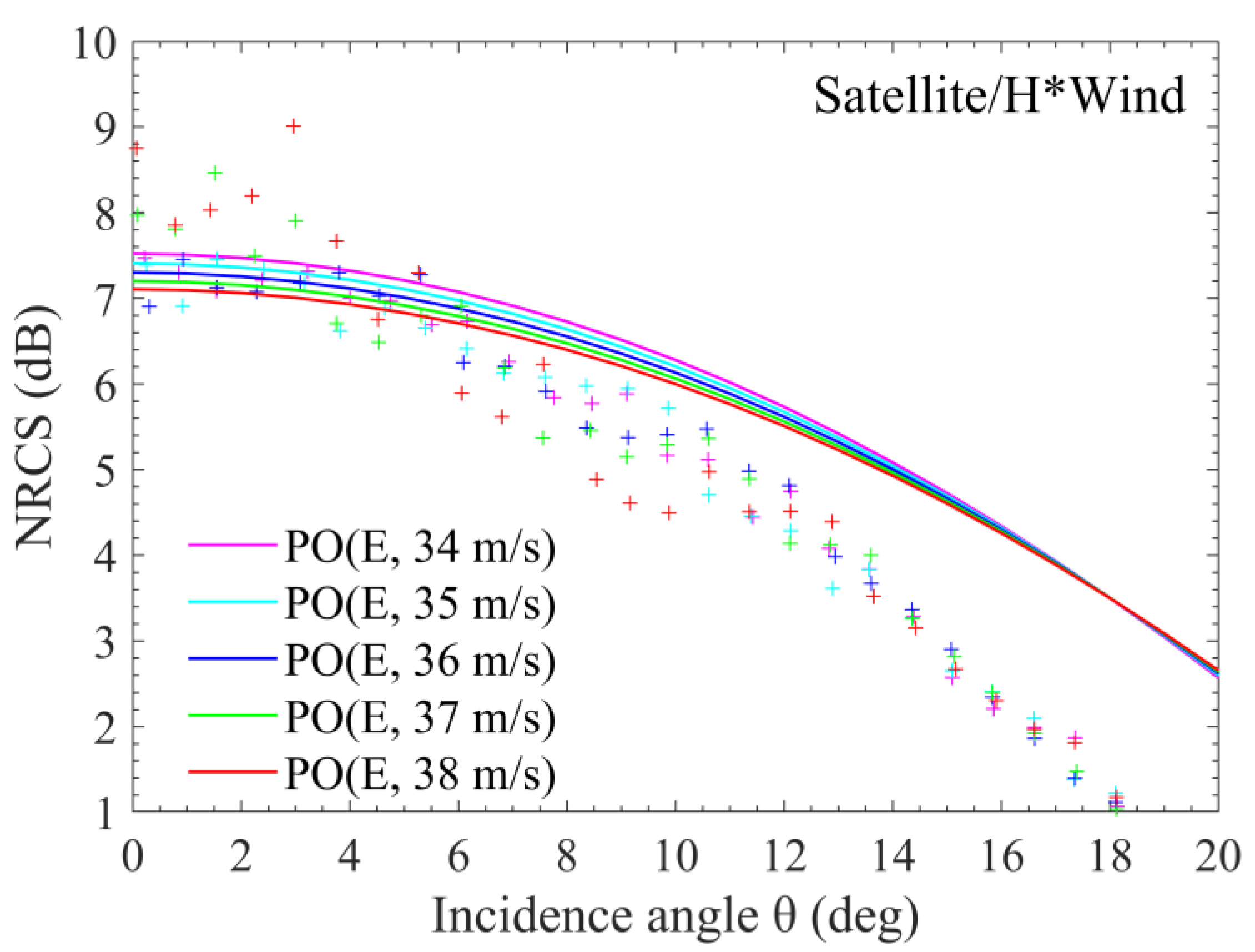
3.3. Further Analysis on the Imapct of Wave Breaking

From Section 3.1, it can be seen that the quasi-specular model is not sufficient to estimate the low-incidence NRCS well for very high winds indicating that the ocean radar backscatter response to various wind conditions cannot be consistently explained by the pure quasi-specular scattering mechanism. As known, ocean wave breaking begins to occur at moderate winds, and becomes more and more dramatic with the wind speed increasing. Breaking of sea surface waves injects air into the water forming foam, spray, and bubbles, which can alter the frictional and roughness characteristics of the ocean surface [54]. Wave breaking is believed to be another significant cause for the behavior of the NRCS at low incidence angles under moderate to severe wind conditions. Here, we will conduct a further discussion on the impact of wave breaking on the low-incidence NRCS response to various wind conditions.

Figure 12 displays the mean values of the NRCS measurements in each (θ, U₁₀) bin as a function of incidence angle for different wind speeds. Figure 12a shows, at wind speeds less than about 20 m/s, the behavior of the NRCS is generally consistent with the standard quasi-specular reflection theory, which holds that the NRCS decreases near nadir and increases near 18°, and its dependence on incidence angle decreases with wind speed increasing. In addition, although wave breaking has already occurred, its effects are so small that they are drowned in the quasi-specular scattering contributions. With wind speed exceeding about 20 m/s, some abnormal behaviors that clearly violate the quasi-specular scattering theory occur, for example, the NRCS near 18° remains almost constant or even decreases with wind speed increasing, as seen in Figure 12b,d. This can only be caused by the relatively smooth ocean surface resulting from wave breaking. It has been indicated in [22] that the wave breaking can reduce the drag coefficient and make the ocean surface at high winds relatively smooth. At nadir, the rougher the sea surface, the lower the NRCS, whereas near 18°, the opposite is true. The wave breaking contributions, which become visible at wind speeds larger than about 20 m/s, increase with wind speed increasing, and have become dominant when wind speed exceeds about 37 m/s.

As shown in Figure 12c, the NRCS is almost insensitive to wind speed and approximately depends linearly on the incidence angle at extremely high wind speeds larger than about 37 m/s. The NRCSs are averaged over the extreme wind speed range of 37–45 m/s at different incidence angles with the Satellite/H*Wind data and plotted versus the incidence angle in Figure 13. In addition, the result can be fitted to:

$${\sigma }_{\mathrm{dB}}^0=10\cdot {\log }_{10}\left({\sigma }^0\right)=a\theta +b$$

(12)

where ${\sigma }_{\mathrm{dB}}^0$ is the NRCS in dB, σ⁰ is the NRCS in natural units, θ is the incidence angle in degrees, a and b are the coefficient to be determined by fitting. Here, the values a = −0.3958 and b = 8.7875 are obtained. Their magnitudes are both much smaller than the results given in [22] possibly due to the fact that the NRCS from PR and KuPR flagged as rain free is selected here whereas that is not the case in [22].

4. Discussion

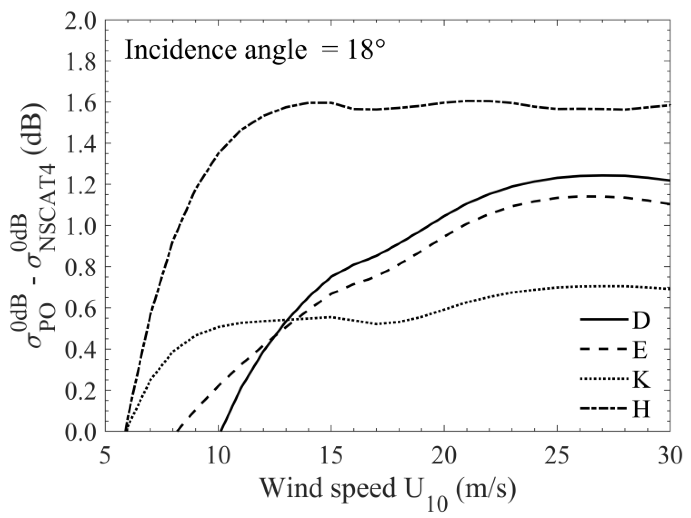
4.1. Impact of Sea State on NRCS

At low winds, the NRCS at small incidence angles is contributed dominantly by the quasi-specular reflection. However, the PO model, which is thought to provide a paradigm for the quasi-specular backscatter, is found to deviate significantly from the measurements. The presence of background swell waves is assumed to be one of the main causes for the large deviations. To discuss the swell effects, we will distinguish the sea wave conditions based on the two separate parameters defined in [55] as:

$$H^{*}=\frac{1}{16}{\left(\frac{g{H}_s}{U_{10}^2}\right)}^2$$

(13)

$${\beta }_{inv}=\frac{U_{10}}{C_p}$$

(14)

where g is the gravity acceleration, H_s is the significant wave height, C_p = ω_p/k_p is the phase velocity of the dominant wave, k_p is the peak wavenumber, ω_p = 2π/T_p is the angular peak frequency, T_p is the peak period. In addition, (ω_p)² = gk_p based on the dispersion relation for surface waves in deep waters. The criteria for distinguishing sea states are that: H* < 3.64 × 10⁻³ and β_inv > 0.82 corresponds to a pure wind sea; H* < 3.64 × 10⁻³ and β_inv < 0.82 is a mixed sea with wind wave dominated; 3.64 × 10⁻³ < H* < 1 and β_inv < 0.82 indicates a mixed sea with swell wave dominated; and H* > 1 and β_inv < 0.82 is a pure swell sea [55].

The satellite/buoy data composed of numerous locations and long time series with widely varying background sea states are used here to investigate the impact of sea states on radar backscatter, and on the performance of the quasi-specular model. Figure 14a illustrates the distribution of the collocated satellite/buoy data in different sea wave conditions. Figure 14b shows the probability of data being in pure wind seas, wind wave dominant seas, swell dominant seas, and pure swell seas with respect to wind speed. Figure 14c shows the magnitude of difference of NRCS between the wind wave seas (including pure wind seas and wind wave dominant seas) and the swell seas (including pure swell seas and swell dominant seas) as a function of incidence angle at different wind speeds. As shown, mixed seas constitute the majority of the dataset. In addition, more than half are in the swell dominant seas. The wind wave seas become dominant only when wind speed exceeds about 9 m/s, whereas at lower winds are mostly the swell dominant seas. In particular, the data are almost in the pure swell seas at wind speeds lower than about 1.5 m/s. Moreover, the impact of existence of swell conditions on radar backscatter that decreases with wind speed is significant at low winds. On the whole, the measurements are mostly in the swell dominant seas and the presence of a swell can significantly modify the NRCS at low winds. As a result, the PO model with wind wave spectrum input cannot accurately reproduce the measured NRCS at low winds without corrections for swell effects.

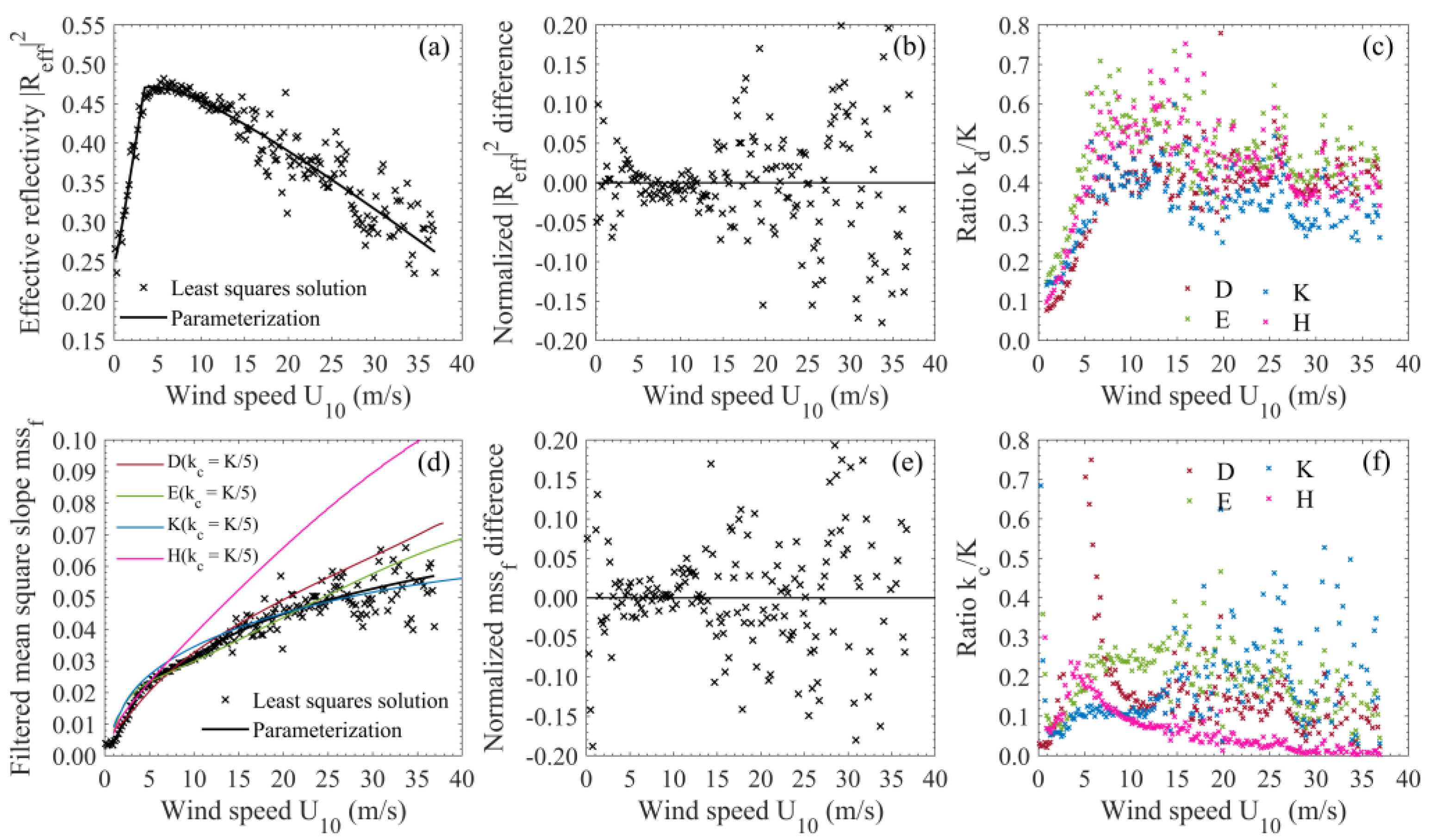
4.2. Impact of Sea State on Radar-Estimated Parameters

Figure 15 displays the radar-estimated effective reflectivity |R_eff|², filtered mean square slope mss_f, total mean square slope mss_t, and effective mean square curvature msc_e versus wind speed at different sea states. It can be seen that the radar-derived values of |R_eff|², mss_f, mss_t, and msc_e are all generally larger in swell cases than in wind sea cases. In light wind conditions (<5 m/s approximately) where the swell cases are dominantly observed, the values of |R_eff|², mss_f, mss_t, and msc_e derived from all the satellite/buoy data are basically identical with those obtained in swell conditions, and their sensitivity to wind speed is the largest. With wind speed increasing, the values from all the data become increasingly close to those in wind sea cases, indicating that the impact of background swell waves is getting smaller. Then, at wind speeds larger than about 10 m/s where the wind sea cases are dominantly observed, the values from all the data are almost the same with those obtained in wind sea cases.

5. Conclusions

The rain-free ocean surface NRCS measurements from the Ku-band PRs onboard the TRMM and GPM satellites with incidence angles ranging from near nadir to approximately 18° and the simultaneous sea surface wind truth from buoy observations, SFMR measurements, and H*Wind analyses over the period from August 2001 to December 2018 are collocated and used to investigate the abilities of three quasi-specular scattering models, i.e., PO, GO, and GO4, to reproduce the Ku-band NRCS at low incidence angles of 0–18° over the wind speed range of 0–45 m/s. On this basis, the limitations of the quasi-specular scattering theory and the effects of wave breaking are discussed in detail.

The PO model, which is assumed to provide a paradigm for the low-incidence quasi-specular backscatter, is found to have poorer performance at low winds, which might be partly improved by optimizing the parameters of the wind-wave spectrum and considering the additional effects of swell waves. At moderate winds, the PO model remains rather accurate in the first 10° of incidence and has a slightly overestimation at higher incidence angles probably due to the neglect of non-Gaussian effects. With wind speed increasing, the PO model can work well at lower and lower incidence angles, and its overestimation at a higher incidence somewhat increases probably resulting from the increasing impact of wave breaking. When wind speed exceeds about 37 m/s, the PO model fails to describe the wind speed insensitivity and linear incidence angle dependence of the NRCS implying that the wave breaking effects have become dominant. The GO4 model can achieve accuracies on the order of magnitude of the PO model, and even can bring a slight improvement at incidence angles less than about 12° for its data-based parameters and absorption of some non-Gaussian effects. The GO model appears to be accurate over the incidence angles of 0–15° for wind speeds up to 37 m/s. At higher incidence, its predictions fall below the measured values due to the missing contributions of Bragg scattering by short waves. It exhibits better performance than the PO and GO4 models at moderate to high winds.

The impact of wave breaking on the behavior of the Ku-band ocean surface radar backscatter at low incidence angles is further discussed. At wind speeds less than about 20 m/s, the NRCS generally behaves in line with the standard quasi-specular reflection theory, whereas some abnormal behaviors occur at higher winds, which can only be attributed to the effects of wave breaking. That is, the wave breaking effects become visible when wind speed exceeds about 20 m/s. The wave breaking contributions increase with the wind speed increasing, and have become dominant at wind speeds larger than about 37 m/s, where the NRCS is insensitive to wind speed and depends linearly on the incidence angle. This paper will provide a basis for the geophysical interpretation of the Ku-band ocean backscattering measurements at low incidence angles. The impact of non-Gaussianity and azimuth on the low-incidence NRCS under different wind conditions that are ignored in this paper will be analyzed in the future.

References

1. Hauser, D.; Tison, C.; Amiot, T.; Delaye, L.; Corcoral, N.; Castillan, P. SWIM: The first spaceborne wave scatterometer. IEEE Trans. Geosci. Remote Sens. 2017, 55, 3000–3014. [Google Scholar] [CrossRef] [Green Version]
2. Abdalla, S. Ku-band radar altimeter surface wind speed algorithm. Mar. Geod. 2012, 35, 276–298. [Google Scholar] [CrossRef] [Green Version]
3. Yang, J.; Ren, L.; Wang, J.; Zheng, G.; Li, X. Preliminary retrieval of ocean winds and waves from Chinese newly launched spaceborne microwave sensors. In Proceedings of the 2017 IEEE International Geoscience and Remote Sensing Symposium (IGARSS), Fort Worth, TX, USA, 23–28 July 2017. [Google Scholar]
4. Valenzuela, G. Theories for the interaction of electromagnetic and oceanic waves—A review. Bound. Layer Meteorol. 1978, 13, 61–85. [Google Scholar] [CrossRef]
5. Barrick, D. Rough surface scattering based on the specular point theory. IEEE Trans. Antennas Propagat. 1968, 16, 449–454. [Google Scholar] [CrossRef]
6. Brown, G. Quasi-specular scattering from the air-sea interface. In Surface Waves and Fluxes; Springer: Dordrecht, The Netherlands, 1990; pp. 1–39. [Google Scholar]
7. Boisot, O.; Nouguier, F.; Chapron, B.; Guérin, C. The GO4 model in near-nadir microwave scattering from the sea surface. IEEE Trans. Geosci. Remote Sens. 2015, 53, 5889–5900. [Google Scholar] [CrossRef] [Green Version]
8. Elfouhaily, T.; Guérin, C. A critical survey of approximate scattering wave theories from random rough surfaces. Waves Random Media 2004, 14, R1–R40. [Google Scholar] [CrossRef]
9. Cox, C.; Munk, W. Measurement of the roughness of the sea surface from photographs of the sun’s glitter. J. Opt. Soc. Am. 1954, 44, 838–850. [Google Scholar] [CrossRef]
10. Brown, G. Backscattering from a Gaussian-distributed perfectly conducting rough surface. IEEE Trans. Antennas Propagat. 1978, 26, 472–482. [Google Scholar] [CrossRef] [Green Version]
11. Freilich, M.; Vanhoff, B. The relationship between winds, surface roughness, and radar backscatter at low incidence angles from TRMM precipitation radar measurements. J. Atmos. Ocean. Technol. 2003, 20, 549–562. [Google Scholar] [CrossRef]
12. Thompson, D.; Elfouhaily, T.; Garrison, J. An improved geometrical optics model for bistatic GPS scattering from the ocean surface. IEEE Trans. Geosci. Remote Sens. 2005, 43, 2810–2821. [Google Scholar] [CrossRef]
13. Bringer, A.; Guérin, C.; Chapron, B.; Mouche, A. Peakedness effects in near-nadir radar observations of the sea surface. IEEE Trans. Geosci. Remote Sens. 2012, 50, 3293–3301. [Google Scholar] [CrossRef]
14. Hauser, D.; Caudal, G.; Guimbard, S.; Mouche, A. A study of the slope probability density function of the ocean waves from radar observations. J. Geophys. Res. Ocean. 2008, 113, 710–713. [Google Scholar] [CrossRef] [Green Version]
15. Boisot, O.; Pioch, S.; Fatras, C.; Caulliez, G.; Bringer, A.; Borderies, P.; Lalaurie, J.; Guérin, C. Ka-band backscattering from water surface at small incidence: A wind-wave tank study. J. Geophys. Res. Ocean. 2015, 120, 3261–3285. [Google Scholar] [CrossRef]
16. Ping, C.; Gang, Z.; Hauser, D.; Fei, X. Quasi-Gaussian probability density function of sea wave slopes from near nadir Ku-band radar observations. Remote Sens. Environ. 2018, 217, 86–100. [Google Scholar]
17. Donnelly, W.; Carswell, J.; Mcintosh, R.; Chang, P.; Wilkerson, J.; Marks, F.; Black, P. Revised ocean backscatter models at C and Ku band under high-wind conditions. J. Geophys. Res. Ocean. 1999, 104, 11485–11497. [Google Scholar] [CrossRef]
18. Fernandez, D.; Carswell, J.; Frasier, S.; Chang, P.; Black, P.; Marks, F. Dual-polarized C- and Ku-band ocean backscatter response to hurricane-force winds. J. Geophys. Res. 2006, 111, 1–17. [Google Scholar] [CrossRef] [Green Version]
19. Sapp, J.; Chang, P.; Jelenak, Z.; Frasier, S.; Hartley, T. Sea-surface NRCS observations in high winds at low incidence angles. In Proceedings of the 2015 IEEE International Geoscience and Remote Sensing Symposium (IGARSS), Milan, Italy, 26–31 July 2015. [Google Scholar]
20. Kudryavtsev, V.; Hauser, D.; Caudal, G.; Chapron, B. A semi-empirical model of the normalized radar cross section of the sea surface 1. Background model. J. Geophys. Res. 2003, 108, 2-1–2-24. [Google Scholar]
21. Quilfen, Y.; Tournadre, J.; Chapron, B. Altimeter dual-frequency observations of surface winds, waves, and rain rate in tropical cyclone Isabel. J. Geophys. Res. Ocean. 2006, 111, 1–13. [Google Scholar] [CrossRef] [Green Version]
22. Li, X.; Zhang, B.; Mouche, A.; He, Y.; Perrie, W. Ku-band sea surface radar backscatter at low incidence angles under extreme wind conditions. Remote Sens. 2017, 9, 474. [Google Scholar] [CrossRef] [Green Version]
23. NASDA Earth Observation Center. TRMM Data Users Handbook; National Space Development Agency of Japan: Hiki-gun, Japan, 2001. [Google Scholar]
24. Hou, A.; Kakar, R.; Neeck, S.; Azarbarzin, A.; Kummerow, C.; Kojima, M.; Nakamura, K.; Oki, R.; Iguchi, T. The global precipitation measurement mission. Bull. Amer. Meteorol. Soc. 2014, 95, 701–722. [Google Scholar] [CrossRef]
25. Liao, L.; Meneghini, R. Validation of TRMM precipitation radar through comparison of its multiyear measurements with ground-based radar. J. Appl. Meteorol. Climatol. 2009, 48, 804–817. [Google Scholar] [CrossRef] [Green Version]
26. Evans, D.; Conrad, C.; Paul, F. Handbook of Automated Data Quality Control Checks and Procedures; NOAA National Data Buoy Center Tech: Stennis Space Center, MS, USA, 2009.
27. Liu, W.; Tang, W. Equivalent Neutral Wind; NASA Jet Propulsion Laboratory: Pasadena, CA, USA, 1996.
28. Uhlhorn, E.; Black, P.; Franklin, J.; Goodberlet, M.; Carswell, J.; Goldstein, A. Hurricane surface wind measurements from an operational stepped frequency microwave radiometer. Mon. Weather Rev. 2007, 135, 3070–3085. [Google Scholar] [CrossRef] [Green Version]
29. Klotz, B.; Uhlhorn, E. Improved stepped frequency microwave radiometer tropical cyclone surface winds in heavy precipitation. J. Atmos. Ocean. Technol. 2014, 31, 2392–2408. [Google Scholar] [CrossRef]
30. Sapp, J.; Alsweiss, S.; Jelenak, Z.; Chang, P.; Carswell, J. Stepped frequency microwave radiometer wind-speed retrieval improvements. Remote Sens. 2019, 11, 214. [Google Scholar] [CrossRef] [Green Version]
31. Powell, M.; Houston, S.; Amat, L.; Morisseau-Leroy, N. The HRD real-time hurricane wind analysis system. J. Wind. Eng. Ind. Aerodyn. 1998, 77, 53–64. [Google Scholar] [CrossRef]
32. Dinapoli, S.; Bourassa, M.; Powell, M. Uncertainty and intercalibration analysis of H*Wind. J. Atmos. Ocean. Technol. 2012, 29, 822–833. [Google Scholar] [CrossRef]
33. Li, S.; Shen, H.; Hou, Y.; He, Y.; Bi, F. Sea surface wind speed and sea state retrievals from dual-frequency altimeter and its preliminary application in global view of wind-sea and swell distributions. Int. J. Remote Sens. 2018, 39, 3076–3093. [Google Scholar] [CrossRef]
34. Plant, W. A stochastic multiscale model of microwave backscatter from the ocean. J. Geophys. Res. Ocean. 2002, 107, 3-1–3-21. [Google Scholar] [CrossRef]
35. Plant, W. Effects of wind variability on scatterometry at low wind speeds. J. Geophys. Res. 2000, 105, 16899–16910. [Google Scholar] [CrossRef]
36. Elfouhaily, T.; Chapron, B.; Katsaros, K.; Vandemark, D. A unified directional spectrum for long and short wind-driven waves. J. Geophys. Res. 1997, 102, 15781–15796. [Google Scholar] [CrossRef]
37. Kudryavtsev, V.; Makin, V.; Chapron, B. Coupled sea surface-atmosphere model 2. Spectrum of short wind waves. J. Geophys. Res. 1999, 104, 7625–7639. [Google Scholar] [CrossRef]
38. Yurovskaya, M.; Dulov, V.; Chapron, B.; Kudryavtsev, V. Directional short wind wave spectra derived from the sea surface photography. J. Geophys. Res. Ocean. 2013, 118, 4380–4394. [Google Scholar] [CrossRef]
39. Hwang, P.; Wang, D. An empirical investigation of source term balance of small scale surface waves. Geophys. Res. Lett. 2004, 31, L15301-1–L15301-5. [Google Scholar] [CrossRef]
40. Hwang, P. Observations of swell influence on ocean surface roughness. J. Geophys. Res. 2008, 113, C12024-1–C12024-14. [Google Scholar] [CrossRef]
41. Hwang, P.; Burrage, D.; Wang, D.; Wesson, J. Ocean surface roughness spectrum in high wind condition for microwave backscatter and emission computations. J. Atmos. Ocean. Tech. 2013, 30, 2168–2188. [Google Scholar] [CrossRef]
42. Hwang, P.; Fois, F. Surface roughness and breaking wave properties retrieved from polarimetric microwave radar backscattering. J. Geophys. Res. Ocean. 2015, 120, 3640–3657. [Google Scholar] [CrossRef]
43. Hwang, P.; Sletten, M.; Toporkov, J. Analysis of radar sea return for breaking wave investigation. J. Geophys. Res. 2008, 113, C02003-1–C02003-16. [Google Scholar] [CrossRef]
44. Wentz, F.; Smith, D.; Mears, C.; Gentemann, C. Advanced algorithms for QuikScat and SeaWinds/AMSR. In Proceedings of the 2001 IEEE International Geoscience and Remote Sensing Symposium (IGARSS), Sydney, Australia, 9–13 July 2001. [Google Scholar]
45. Hersbach, H.; Stoffelen, A.; Haan, S. An improved C-band scatterometer ocean geophysical model function: CMOD5. J. Geophys. Res. Ocean. 2005, 572, 1–18. [Google Scholar] [CrossRef]
46. Isoguchi, O.; Shimada, M. An L-band ocean geophysical model function derived from PALSAR. IEEE Trans. Geosci. Remote Sens. 2009, 47, 1925–1936. [Google Scholar] [CrossRef]
47. Yueh, S.; Dinardo, S.; Fore, A.; Li, F. Passive and active L-band microwave observations and modeling of ocean surface winds. IEEE Trans. Geosci. Remote Sens. 2010, 48, 3087–3100. [Google Scholar] [CrossRef]
48. Yan, Q.; Zhang, J.; Fan, C.; Meng, J. Analysis of Ku-and Ka-band sea surface backscattering characteristics at low-incidence angles based on the GPM dual-frequency precipitation radar measurements. Remote Sens. 2019, 11, 754. [Google Scholar] [CrossRef] [Green Version]
49. Majurec, N.; Johnson, J.; Tanelli, S.; Durden, S. Comparison of model predictions with measurements of Ku- and Ka-band near-nadir normalized radar cross sections of the sea surface from the Genesis and Rapid Intensification Processes experiment. IEEE Trans. Geosci. Remote Sens. 2013, 52, 5320–5332. [Google Scholar] [CrossRef]
50. Verhoef, A.; Stoffelen, A. Algorithm Theoretical Basis Document for the OSI SAF Wind Products Version 1.7; Ocean and Sea Ice SAF, Royal Netherlands Meteorological Institute: De Bilt, The Netherlands, 2018. [Google Scholar]
51. Yan, Q.; Zhang, J.; Fan, C.; Wang, J.; Meng, J. Study of sea surface slope distribution and its effect on radar backscatter based on GPM Ku-band precipitation radar measurements. J. Appl. Remote Sens. 2018, 12, 1–16. [Google Scholar] [CrossRef] [Green Version]
52. Ulaby, F.; Long, D. Microwave Radar and Radiometric Remote Sensing; University of Michigan Press: Ann Arbor, MI, USA, 2014. [Google Scholar]
53. Jackson, F.; Walton, W.; Hines, D.; Walter, B.; Peng, C. Sea surface mean square slope from Ku-band backscatter data. J. Geophys. Res. 1992, 97, 11411–11427. [Google Scholar] [CrossRef]
54. Donelan, M.; Haus, B.; Reul, N.; Plant, W.; Stiassnie, M.; Graber, H.; Brown, O.; Saltzman, E. On the limiting aerodynamic roughness of the ocean in very strong winds. Geophys. Res. Lett. 2004, 31, 1–5. [Google Scholar] [CrossRef] [Green Version]
55. Chu, X.; He, Y.; Chen, G. Asymmetry and Anisotropy of Microwave Backscatter at Low Incidence Angles. IEEE Trans. Geosci. Remote Sens. 2012, 50, 4014–4024. [Google Scholar] [CrossRef]
Figure 1. Azimuthally integrated ocean surface curvature spectra B(k): (a) The D spectrum with wind speed fluctuation of 1.5 m/s standard deviation, (b) the E spectrum, (c) the K spectrum, and (d) the H spectrum. The lines from inside out correspond to wind speeds of 1, 3, 5, 10, 15, 20, 30, 40, and 50 m/s.
Remotesensing 12 03445 g001
Figure 2. Examples of predictions of the physical optics (PO) model with D (solid curve), E (dashed curve), K (dotted curve), and H (dash-dotted curve) spectra input and their comparison with the bin-averaged normalized radar cross-section (NRCS) measurements. Results are plotted as functions of incidence angle for wind speeds of 1, 3, 9, 15, 21, 27, 33, 39, and 45 m/s. Symbols for the reference dataset are as follows: Circles are the collocated satellite/buoy data; triangles are the satellite/stepped-frequency microwave radiometer (SFMR) data; and pluses represent the satellite/H*Wind data.
Remotesensing 12 03445 g002
Figure 3. Root mean square error (RMS) differences between the predictions of the PO model with D (solid curve), E (dashed curve), K (dotted curve), and H (dash-dotted curve) spectra input and the bin-averaged NRCS measurements calculated with (a,b) the satellite/buoy data, (c,d) the satellite/SFMR data, and (e,f) the satellite/H*Wind data as functions of incidence angle at (a) low, (b) moderate, (c,e) high, and (d,f) severe winds.
Remotesensing 12 03445 g003
Figure 4. RMS differences between the predictions of the PO model with D (solid curve), E (dashed curve), K (dotted curve), and H (dash-dotted curve) spectra input and the bin-averaged NRCS measurements at all incidence angles as functions of wind speed: (a) The satellite/buoy data are used as reference; (b) the satellite/SFMR data are the reference; and (c) the satellite/H*Wind data are the reference.
Remotesensing 12 03445 g004
Figure 5. Differences between the omnidirectional PO computations (in dB) and the azimuthally averaged NRCSs (in dB) obtained with NSCAT4 HH GMF as functions of wind speed at an incidence angle of 18°. Curve style sequence for D, E, K, and H spectra is solid, dashed, dotted, and dash-dotted.
Remotesensing 12 03445 g005
Figure 6. Comparison of the PO model computations using the E spectrum (solid lines) with the bin-averaged NRCS measurements calculated with the satellite/H*Wind data (pluses) at wind speeds of 34–38 m/s in 1 m/s intervals. Color sequence for the increasing wind speed is magenta, cyan, blue, green, and red.
Remotesensing 12 03445 g006
Figure 7. Least squares fits of the classical geometrical optics GO (solid lines) and improved geometrical optics GO4 (dotted lines) models and their comparison with measurements at selected wind speeds. Circles represent the satellite/buoy data; triangles are the satellite/SFMR data; and pluses are the satellite/H*Wind data. Red indicates that the data are used for the fits.
Remotesensing 12 03445 g007
Figure 8. RMS differences between the NRCSs computed with the fitted GO (solid lines) and GO4 (dotted lines) models and the bin-averaged NRCS measurements from (a,b) the satellite/buoy data, (c,d) the satellite/H*Wind data, and (e,f) the satellite/SFMR data as functions of incidence angle at different wind conditions.
Remotesensing 12 03445 g008
Figure 9. RMS differences between the NRCSs computed with the fitted GO (solid lines) and GO4 (dotted lines) models and the bin-averaged NRCS measurements from (a) the satellite/buoy data, (b) the satellite/H*Wind data, and (c) the satellite/SFMR data at all incidence angles as functions of wind speed.
Remotesensing 12 03445 g009
Figure 10. (a) Least squares solutions for |Reff|2 with the GO model (crosses) and the corresponding parameterization based on a least square fitting of the solutions at 0 < U10 < 37 m/s (black line). (b) Parameterization accuracy: Parameterized |Reff|2/|Reff|2 − 1. (c) Ratio of the low-limit cutoff wave number kd to the radar wave number K as a function of wind speed for the D, E, K, and H spectra. (d) Solutions for the filtered mss (crosses), the best-fit parameterization (black line), and their comparison with those obtained by integrating the D, E, K, and H spectral functions from zero to an upper cutoff wave number kc = K/5. (e) Parameterization accuracy: Parameterized mssf/mssf − 1. (f) Ratio of kc to K versus wind speed. Color sequence for D, E, K, and H spectra is dark red, olive green, dodger blue, and deep pink.
Remotesensing 12 03445 g010
Figure 11. (a) Least squares solutions for the total mss with the GO4 model (crosses), the best-fit parameterization (black line), and their comparison with the total mean square slopes from the clean water sun glitter data reported in [9] (squares) and those obtained by integrating the D, E, K, and H spectral functions from zero to 2000 rad/m. (b) Parameterization accuracy: Parameterized msst/msst – 1. (c) Solutions for the effective msc (crosses) and the best-fit parameterization (black line). (d) Parameterization accuracy: Parameterized msce/msce – 1. (e) Ratio of the high-limit cutoff wave number kr to K versus wind speed. Colors for D, E, K, and H spectra are the same as those in Figure 10.
Remotesensing 12 03445 g011
Figure 12. Bin-averaged NRCS measurements as a function of incidence angle for different wind speeds: (a) The satellite/buoy data, and (b,c) the satellite/H*Wind data. (d) Enlarged view of the black frame in (b). Symbol types and colors indicate different wind speeds.
Remotesensing 12 03445 g012
Figure 13. NRCS dependence on incidence angle at extremely high winds. Pluses are the NRCS values averaged over 37 m/s ≤ U10 ≤ 45 m/s at different incidence angles. Overlaid is the linear regression fit.
Remotesensing 12 03445 g013
Figure 14. (a) Distribution of the satellite/buoy data in different wave conditions. (b) Probability of the data being in pure wind seas (black pluses), wind wave dominant seas (blue triangles), swell dominant seas (green circles), and pure swell seas (red squares) with respect to wind speed. (c) Magnitude of the difference of NRCS between the wind wave seas and the swell seas as a function of incidence angle at different wind speeds.
Remotesensing 12 03445 g014
Figure 15. Radar-estimated (a) effective reflectivity |Reff|2, (b) filtered mean square slope mssf, (c) total mean square slope msst, and (d) effective mean square curvature msce as functions of wind speed. Red squares correspond to the satellite/buoy data acquired during conditions of wind sea (pure wind and wind wave dominant seas); green circles correspond to the data acquired during conditions of swell sea (pure swell and swell dominant seas), and blue crosses correspond to all the satellite/buoy data.
Remotesensing 12 03445 g015
Publisher’s Note: MDPI stays neutral with regard to jurisdictional claims in published maps and institutional affiliations.