A Phase Filtering Method with Scale Recurrent Networks for InSAR


School of Information and Communication Engineering, University of Electronic Science and Technology of China, Chengdu 611731, China
*
Author to whom correspondence should be addressed.
Remote Sens. 2020, 12(20), 3453; https://0-doi-org.brum.beds.ac.uk/10.3390/rs12203453
Submission received: 2 September 2020
/
Revised: 18 October 2020
/
Accepted: 18 October 2020
/
Published: 21 October 2020
(This article belongs to the Special Issue InSAR in Remote Sensing)
Abstract
:Phase filtering is a key issue in interferometric synthetic aperture radar (InSAR) applications, such as deformation monitoring and topographic mapping. The accuracy of the deformation and terrain height is highly dependent on the quality of phase filtering. Researchers are committed to continuously improving the accuracy and efficiency of phase filtering. Inspired by the successful application of neural networks in SAR image denoising, in this paper we propose a phase filtering method that is based on deep learning to efficiently filter out the noise in the interferometric phase. In this method, the real and imaginary parts of the interferometric phase are filtered while using a scale recurrent network, which includes three single scale subnetworks based on the encoder-decoder architecture. The network can utilize the global structural phase information contained in the different-scaled feature maps, because RNN units are used to connect the three different-scaled subnetworks and transmit current state information among different subnetworks. The encoder part is used for extracting the phase features, and the decoder part restores detailed information from the encoded feature maps and makes the size of the output image the same as that of the input image. Experiments on simulated and real InSAR data prove that the proposed method is superior to three widely-used phase filtering methods by qualitative and quantitative comparisons. In addition, on the same simulated data set, the overall performance of the proposed method is better than another deep learning-based method (DeepInSAR). The runtime of the proposed method is only about 0.043s for an image with a size of pixels, which has the significant advantage of computational efficiency in practical applications that require real-time processing.
1. Introduction
In recent decades, the spatial resolution of synthetic aperture radar (SAR) images acquired from space has continuously improved, thanks to the precise orbit control, hardware upgrades, and algorithm advancements in the signal processing field [1]. For example, the spotlight mode of TerraSAR-X has a spatial resolution of 1 m, and its staring spotlight mode even reaches 0.25 m [2]. This breakthrough has brought life to interferometric SAR (InSAR) applications, such as topography mapping and deformation monitoring. Because the acquisition of high-resolution SAR images has become possible, the high-precision measurement of useful geophysical parameters (such as terrain height and surface deformation) can be achieved while using InSAR techniques. Therefore, InSAR is bursting with new research vitality.
In the whole InSAR processing chain, the accuracy of the obtained terrain height is highly related to phase unwrapping, but the presence of noise in the interferometric phase increases the difficulty of unwrapping and reduces the accuracy of unwrapping. Therefore, it is necessary to filter the interferometric phase before unwrapping to reduce noise. In the process of filtering noise, it is essential to preserve good phase detail features (such as phase fringe edges), which determines the accuracy of the obtained terrain height. At the same time, in order to meet the requirements of quickly obtaining height products in practical applications, the computational efficiency of the filtering algorithm should be as high as possible. It is worth noting that the ideal filtering effect is to completely separate the phase and noise from the noisy interferometric phase, but the filtering algorithm cannot achieve this ideal state [3]. Therefore, researchers are committed to continuously developing filtering algorithms that can efficiently filter out noise as much as possible while preserving the fine detail features.
The widely-used phase filtering methods can be grouped into three categories: spatial domain, transform domain, and nonlocal (NL) methods. One typical spatial domain method is the Lee filter which filters out noise along fringes adaptively according to the local noise statistics and directionally dependent windows [4]. Based on the basic Lee filter, several improved versions have appeared afterward [5,6,7,8]. For example, a directionally adaptive method is proposed in [6]. The length and width of the filter window can continuously change with the fringe density, and the direction can be changed according to the fringe direction. Examining these filters carefully, they are trying to increase the capacity to preserve the phase detail based on an adaptive windowing process of the interferometric phase, but this window processing operation may cause fringe detail loss due to excessive smoothing and it requires heavy processing time.
The transform domain method is usually divided into the frequency domain and wavelet domain. The first frequency domain method was proposed by Goldstein and Werner in [9]. The method can smooth the interferometric phase while using the bandpass characteristic of the filter, because the power spectrum of the interferometric phase is typically the sum of a narrow-band component combined with broad-band noise. A modified version of the Goldstein filter is presented in [10], which enhances the filtering capacity for areas of low coherence by modifying the Goldstein filter parameter according to the value of coherence. Most of the frequency domain methods consider the area with different values of coherence in the filtering process to improve filtering effect, but the filtering result of the low coherence area still needs to be improved [10,11,12,13]. Besides, the first wavelet domain method for interferometric phase filtering is proposed in [14], which reduces noise in the complex wavelet plane. This work has important implications for subsequent research [15,16]. Generally speaking, wavelet domain filters have a better capacity to preserve spatial resolution when compared with spatial domain methods.
Generally speaking, when comparing the above two types of methods, the transform domain method may have a stronger capacity to preserve phase details, while the spatial domain method has a stronger capacity to suppress noise. Therefore, researchers continue to pursue better performance by fully mining more useful information from the interferometric phase. In order to improve the capacity to preserve phase details, the NL-means algorithm [17,18,19] has been successfully applied to the fields of InSAR [20,21,22,23,24]. The first NL-InSAR approach for the estimation of the interferometric phase is proposed in [20], which derives a patch-similarity criterion that is suitable for the interferogram and performs the weighted averaging of similar pixels defined by the criterion. In order to address the inherent diversity of natural terrain in generating digital elevation models (DEMs) process, an NL-InSAR filter is proposed in [25], which can adjust the filtering parameters adaptively to ensure the fine filtering effect. Combining the non-local approach, wavelet transform, and Wiener filtering, an InSAR block-matching 3D filtering method, called InSAR-BM3D, is proposed in [26], which preserves phase structures well. When compared with the above two types of methods, this type of method may achieve better filtering effects. However, due to a large number of similar area search operations, this type of method sacrifices computational efficiency.
In recent years, deep learning has been successfully applied to many fields, such as machine vision, optical image processing [27,28,29,30], and SAR image denoising [31,32,33]. In addition, the research of deep learning in the field of interferometric SAR has also begun to sprout [34,35,36]. In this paper, we propose a deep learning-based method to filter the interferometric phase for InSAR, which can better balance the noise suppression capacity and phase detail preservation capacity in order to obtain higher-precision results and ensure computational efficiency. In order to preserve the range () of the interferometric phase, the filtering is implemented on the real and imaginary parts of the interferometric phase. In this method, the real and imaginary parts of the interferometric phase are filtered using a scale recurrent network, called phase filtering network (PFNet), which includes three single scale subnetworks that are based on the encoder-decoder architecture. The network can utilize the global structural phase information that is contained in the different-scaled feature maps, because RNN units are used to transmit current state information among different subnetworks. The encoder part is used for extracting the phase features, and the decoder part restores detailed information from the encoded feature maps and makes the size of the output image the same as that of the input image. Experiments on simulated and real InSAR data prove that the proposed method is superior to three widely-used phase filtering methods by qualitative and quantitative comparisons and it has the significant advantage of computational efficiency.
The remainder of the paper is organized, as follows. In Section 2, we describe the necessity and particularity of the interferometric phase filtering in InSAR. A data generation method, the proposed method, and evaluation indexes are described in Section 3, and experiments that are based on simulated and real InSAR data are implemented in order to evaluate the proposed method with the other three widely-used methods in Section 4. The conclusion is presented in Section 5.
2. Problem Description
This section describes, in detail, why the interferometric phase filtering is required in the InSAR processing chain, the particularity of the interferometric phase filtering when compared to general image filtering, and the noise model of the interferometric phase in InSAR. At the same time, this section provides a theoretical basis for generating simulated data.
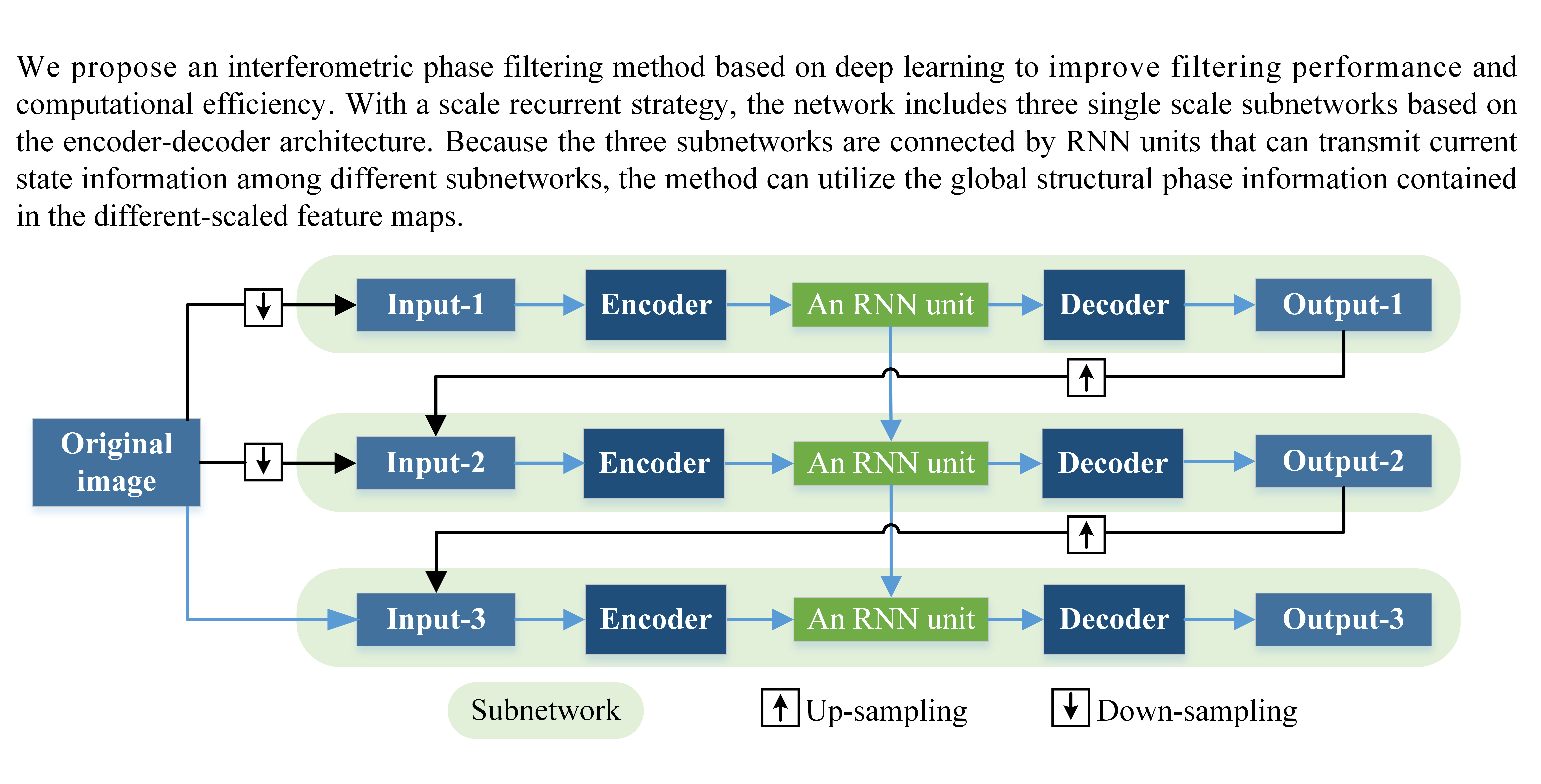
InSAR is a technique that exploits the interferometric phase of two or more coregistered single look complex (SLC) SAR images to acquire useful information, such as relative height and surface deformation [37]. These images are usually obtained by means of different antennas or repeat-pass. Figure 1 shows the commonly used InSAR geometry model in the case of two antennas or passes [1]. The flight direction of the platform is perpendicular to the paper.
Consider any scatterer point s with the surface height h in Figure 1, the unwrapped phase contains two parts: the unwrapped flat-earth phase and the unwrapped height phase , which can be expressed [1,38] as
where is the wavelength of the transmit signal, and are the range from the scatterer point s to the two antenna phase center positions, is the local incident angle, is the angle of the baseline relative to the reference horizontal plane, is the baseline perpendicular to the line of sight, and the factor Q depends on the working model of the antenna. When , one antenna transmits a signal while the two antennas receive the echo at the same time. When , each antenna transmits and receives signals separately, such as space-borne repeat-pass modes. According to Equation (1), as long as is known, the height h can be obtained, because other parameters can be easily obtaining according to system parameters and geometry model. The unwrapped phase can be obtained by unwrapping the ideal interferometric phase after removing the flat-earth phase, and their relationship can be expressed as
where angle(·) returns the phase angle. The real interferometric phase typically contains noise, and the presence of noise increases the difficulty of phase unwrapping and reduces its accuracy, which directly affects the accuracy of the obtained height h. Therefore, interferometric phase filtering is a critical step before unwrapping.
After removing the flat-earth phase, the phase noise can be modeled [4,14,16] as
where is the real interferometric phase, and are two complex SAR images, * represents the complex conjugate, and is the zero-mean additive Gaussian noise and independent from . Figure 1 also shows this process of adding noise. The process of retrieving from is called phase filtering. In simulation experiments, the ideal interferometric phase can be used in order to evaluate the accuracy of filtering.
Because of the periodicity of trigonometric functions, the range of the interferometric phase is , which forms phase fringes in interferometric phase images. In order to correctly calculate the phase gradient in phase unwrapping, phase jumps where the phase goes from to or to should be preserved. Therefore, the direct filtering for the interferometric phase cannot be adopted in the real domain. The interferometric phase is filtered in the complex domain in order to solve this problem. An interferometric phase in the complex domain can be expressed as
The real and imaginary parts of the interferometric phase can be expressed as
After the real and imaginary parts are filtered, the filtered interferometric phase can be obtained by
where , , and are the filtered interferometric phase and its real part and imaginary part, respectively. In the above process, it is ensured that the range of the interferometric phase is not changed while the noise is filtered out. Furthermore, phase jumps are preserved without being smoothed, which is beneficial to the phase gradient estimation in phase unwrapping.
3. Materials and Methods
3.1. Dataset
In practice, it is very difficult to obtain a large number of real interferometric phase images with corresponding clean phase images, while network training usually requires a large number of labeled samples. Therefore, we use a simulation method to generate samples in order to verify the effectiveness of the proposed method and evaluate its performance. This section describes the detailed sample generation process.
In experiments on simulated data, the Gaussian distributed random matrix is used to generate unwrapped phase in order to simulate the diversity of real terrain in nature [39]. When the unwrapped phase is known, we can easily obtain the interferometric phase according to Equation (2). The detailed data generation steps are as follows.
- Generate an initial Gaussian distributed random matrix. The size of the initial matrix is for our simulation experiments.
- Enlarge the matrix to a larger matrix ( pixels for our experiments) using bicubic interpolation and scale its range of values to a larger range (0 to 20 rad for our simulation experiments). The large matrix is considered as the unwrapped phase.
- The real and imaginary parts of the clean and noisy interferometric phase are generated according to Equation (5).
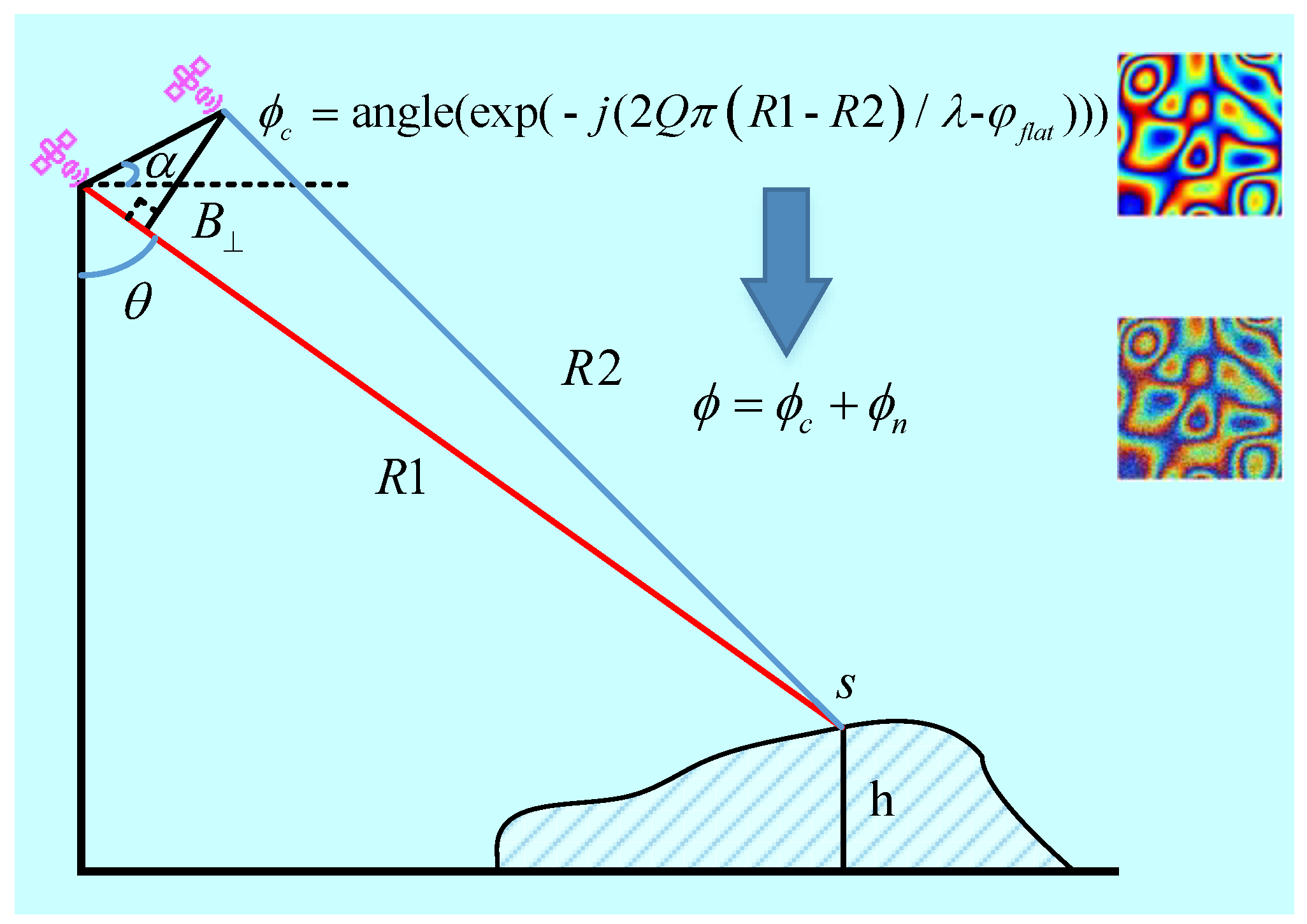
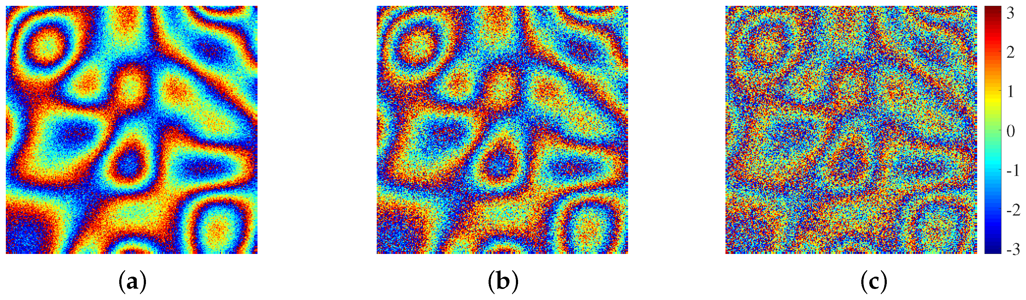
During the generation process, there are three variable parameters, namely the size of the initial random matrix, the range of the unwrapped phase, and the level of added noise. The size of the initial random matrix determines the number of extreme points in the unwrapped phase, so the terrain complexity can be adjusted according to this value. When comparing Figure 2a–c and Figure 2d–f, we can see that, the larger the initial random matrix, the more complex the terrain. Given a fixed size of the initial random matrix, the range of the unwrapped phase determines the fringe density of the corresponding interferometric phase. When comparing Figure 2e,f and Figure 2g,h, it can be seen that the larger the range of the unwrapped phase, the denser the interferometric phase fringe. Furthermore, the level of added noise determines the clarity of the interferometric phase fringe. Figure 3 shows the interferometric phase images containing different levels of noise. Their signal-to-noise ratio (SNR) are 1.17 dB, −0.87 dB and −2.1 dB, respectively. We can see that the stronger the noise, the less clear the phase fringe. Based on the above analysis, it can be seen that these three parameters affect the difficulty of filtering and, the greater their value, the greater the difficulty of filtering.
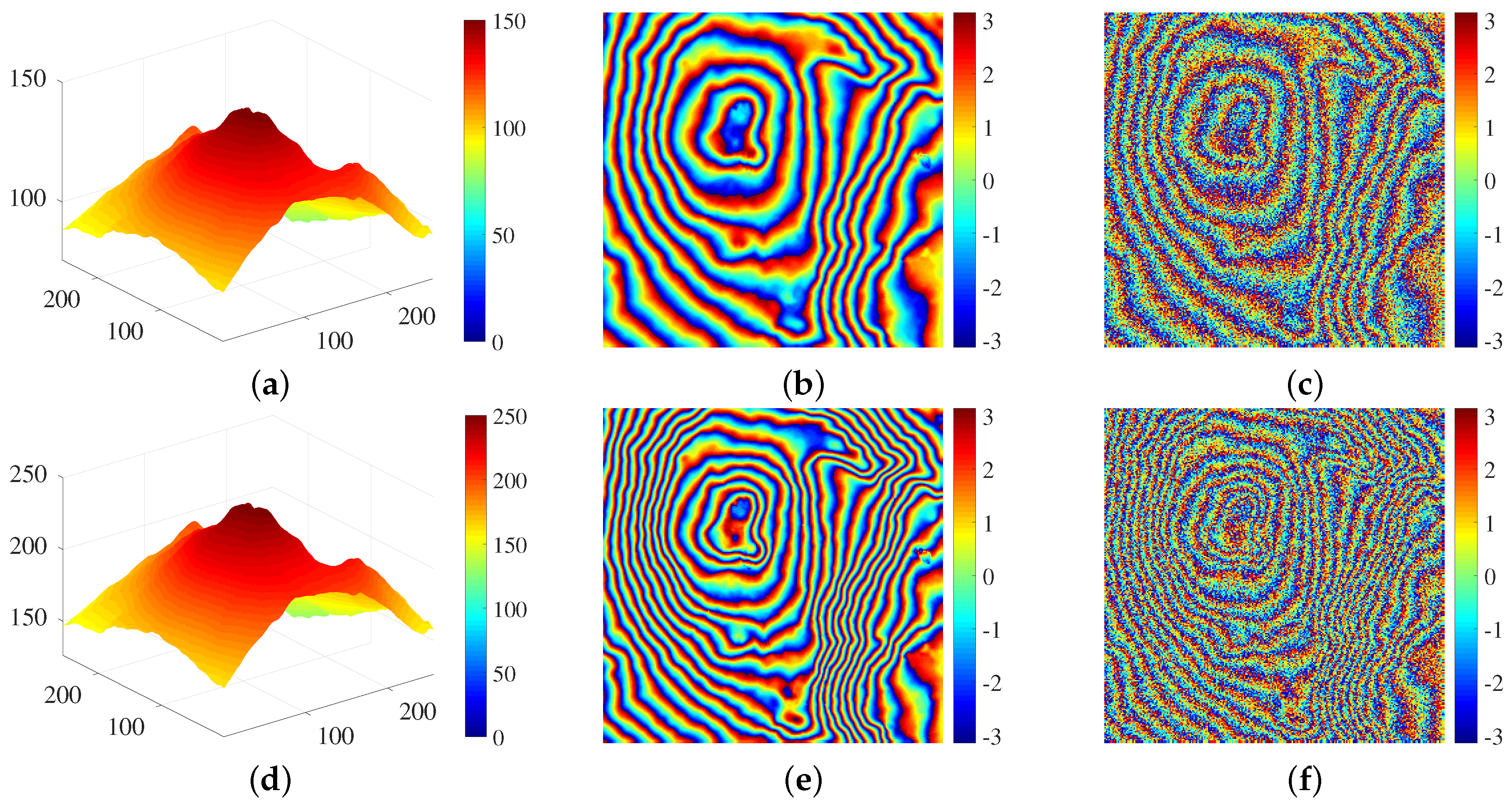
In experiments on real InSAR data, the real DEM is used to generate training samples [40], which can make the training samples similar to the real terrain. This increase in similarity helps to obtain a better filtering performance, because more details can be learned by the network. The real DEM used in this paper comes from EU-DEM v1.1 and it can be downloaded from https://www.eea.europa.eu/data-and-maps/data/copernicus-land-monitoring-service-eu-dem. To augment the training set, we obtain a group of training samples corresponding to different fringe density from one real DEM (etna Volcano, pixels) by scaling its elevation to different degrees. The maximum elevation of the real DEM are scaling from 150 m to 250 m with an interval of 10 m in order to obtain eleven different elevation images considered as unwrapped phase images ((250 − 150)/10 + 1). The unwrapped phase image is converted to the interferometric phase images according to Equation (2), and each interferometric phase image is split into thirty-six small sections ( pixels). Therefore, 396 (36 × 11) interferometric phase images can be obtained. According to the aforementioned steps, 396 (36 × 11) pairs of real part images and 396 pairs of imaginary part images are generated and used as the training set in Section 4.2. Figure 4 shows two examples of using DEMs to generate samples.
3.2. Proposed Method
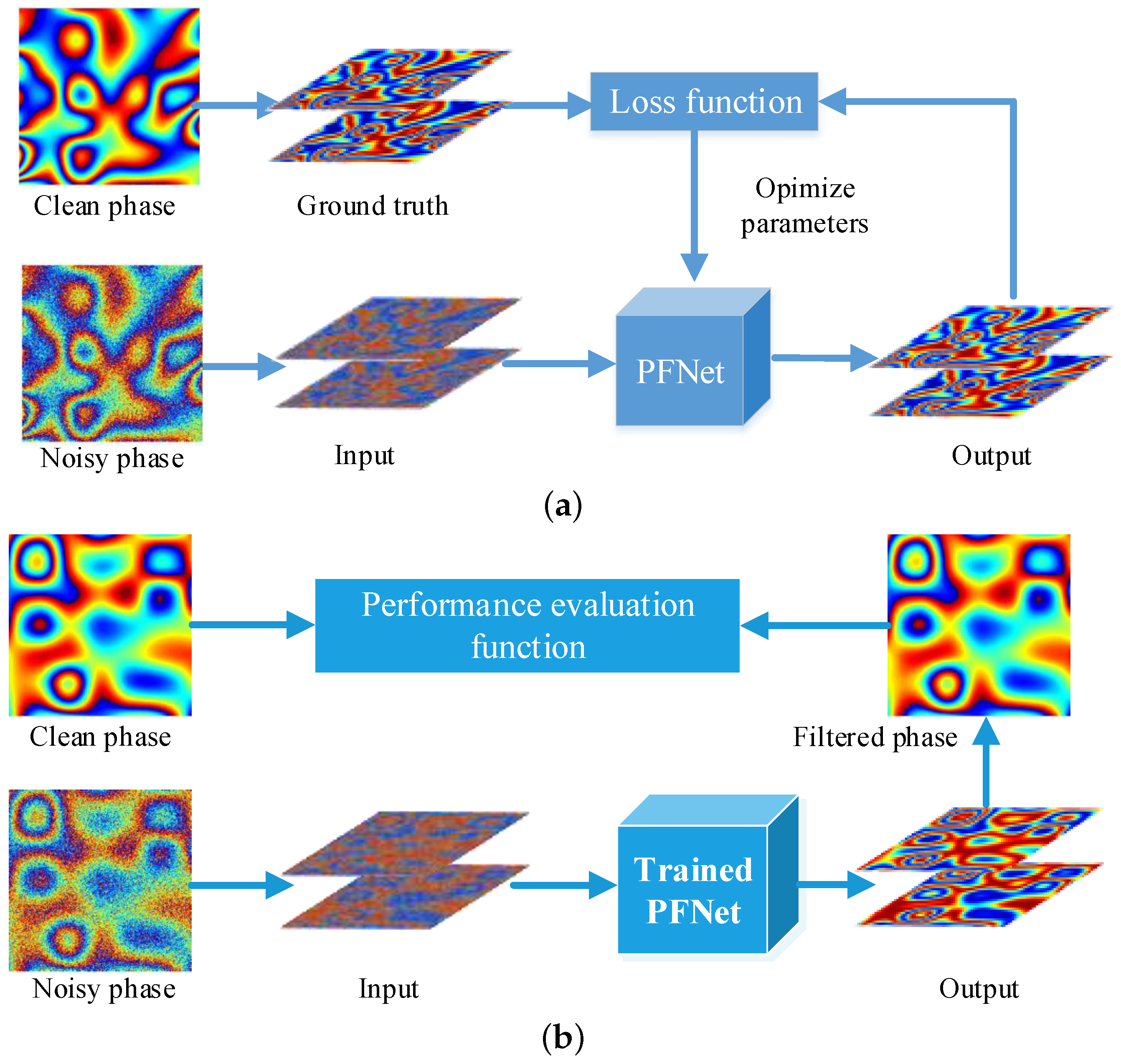
In this paper, an interferometric phase filtering method that is based on deep learning is proposed. The method has two stages, as shown in Figure 5: training and testing process. For the training process, PFNet takes the real part and imaginary part images of the interferometric phase as input and produces the corresponding filtered real part and imaginary part images. The trainable parameters are updated by minimizing the loss function calculated from the network output and the real part and imaginary part images of the clean interferometric phase (ground truth). Adam optimizer [41] is used and the loss function is introduced in the next subsection. For the testing process, the real part and imaginary part images of a noisy interferometric phase are separately fed into the trained PFNet to obtain the filtered real part and imaginary part images. Finally, the corresponding filtered interferometric phase image is obtained according to Equation (6) and it is compared with the clean interferometric phase image in order to analyze filtering performance by performance evaluation functions. Next, we first introduce the overall architecture of PFNet and then describe the network details via the single scale subnetwork.
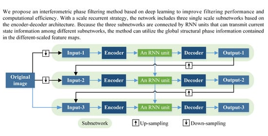
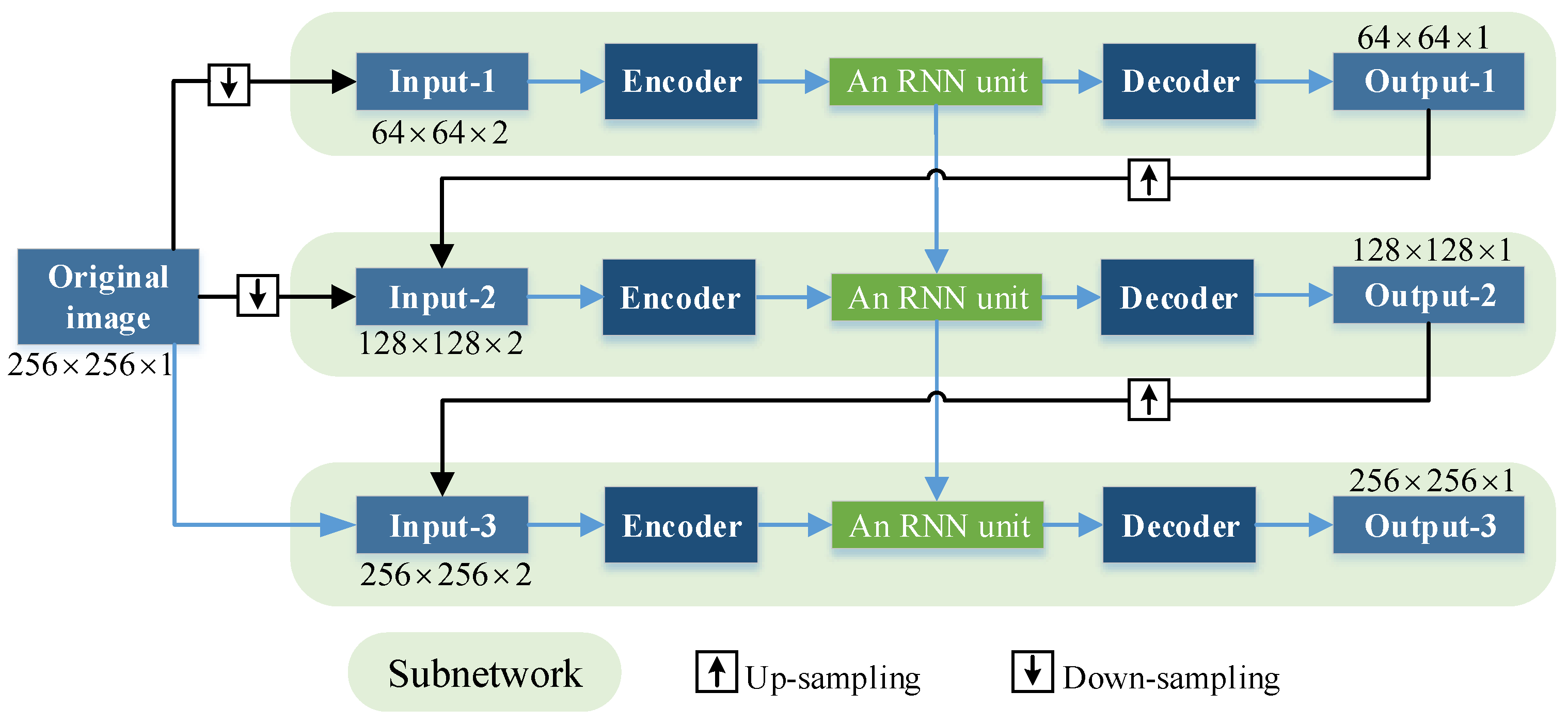
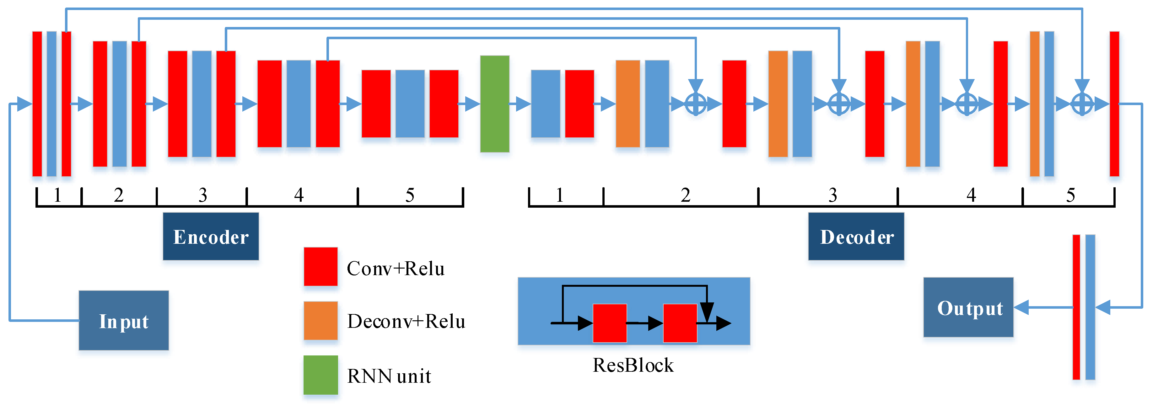
Figure 6 illustrates the overall architecture of PFNet. The network is built based on a scale recurrent structure including three single scale subnetworks, and different subnetworks correspond to different scales of inputs and outputs. The scale of the three subnetworks are , , and , respectively. Each subnetwork consists of input, output, encoder, decoder, and RNN unit. The input of the first subnetwork (Input-1) is two identical down-sampled original images, and the input of the second and third networks (Input-2 and Input-3) is the output of the previous subnetwork and a scaled original image. The un-sampling and down-sampling operation are completed while using bilinear interpolation. RNN units are used to connect different subnetworks, which can transmit the current state information to the RNN unit of the next subnetwork, in order to utilize the global structural phase information contained in the different-scaled feature maps. This facilitates the restoration of a full-resolution clean phase image across scales. RNN units can be different forms, such as long-short term memory (LSTM) [42], gated recurrent unit (GRU) [43], and simple recurrent unit (SRU) [44]. In our method, GRU is selected, since its performance is best in our experiments. In addition, the trainable parameters of each subnetwork are shared, rather than independent, in order to reduce the number of parameters.
Figure 7 illustrates the detailed structure of each subnetwork and Table 1 lists the detailed parameter configuration. Because the input size of different subnetworks are different, for convenience, the width and height of the image are expressed by . The encoder part transforms the input image into the feature maps with a smaller size and more channels, and it contains five encoder blocks. As shown by different colored modules in Figure 7, each encoder block consists of a convolution (Conv) layer, a residual network (ResBlock) [27], and a convolution layer. A convolution layer includes two operations: convolution and rectified linear unit (Relu). In the latter four encoder blocks, the first convolution layer doubles the number of channels of the previous layer and halves the size of its feature map. In the encoder process, the main phase fringe information is captured and, meanwhile, noise is gradually suppressed after each block. On the other hand, the size of the feature map is reduced, which helps to increase the training speed and reduce the demand for computing power. The decoder part restores detailed information from the encoded feature maps and makes the size of the output image the same as that of the input image. It also contains five decoder blocks. The first decoder block consists of a ResBlock and a convolution layer, and the other four blocks have one more deconvolution (Deconv) layer. A deconvolution layer includes two operations: deconvolution and rectified linear unit. In the last four decoder blocks, the first deconvolution layer halves the number of channels of the previous layer and doubles the size of its feature map. In the decoder process, the detail phase information and image size are gradually restored after each block and the size of feature maps gradually returns to that of the input image.
Deep networks are good for enriching the level of features and integrating low/mid/high-level features, but it may be difficult to train [45]. Therefore, two methods are used to avoid the problem. First, in each encoder or decoder block, a Resblock is connected after the first convolution or deconvolution layer in order to accelerate convergence and avoid gradient explosion or gradient disappearance when deepening the network [46]. Besides, a convolution or deconvolution layer is inserted after each Resblock to further increase the network depth. Second, between the encoder and decoder, the feature maps with the same size are added by skip connections [47], which can pass detailed phase information to the top layer and facilitate the gradient propagation. In the decoder process, the feature maps from convolution layers can compensate the main detailed phase information. In other words, these added skip connections can improve network performance and make training easier and more efficient.
3.3. Loss Function
The mean-square error (MSE) between the filtered real part or imaginary part image (network output) and the clean real part or imaginary part image (ground truth) is adopted as the loss function. It can be expressed as
where n is the scale number of the scale recurrent network, is the number of pixels of the i-th scaled images, and are the ground truth and network output in the i-th scale, respectively.
3.4. Performance Evaluation Index
The evaluation of the filtering performance is divided into two aspects: filtering accuracy and computational efficiency, in which the filtering accuracy is evaluated by comprehensively considering the capacities of noise suppression and phase detail preservation. An excellent phase filtering method is usually efficient and it has a sufficient capacity to suppress noise while preserving fine phase detail information. In this paper, qualitative and quantitative evaluation methods are adopted to complete the evaluation task. Qualitative evaluation means that the evaluator performs filtering quality judgment based on visual effects. Therefore, the noisy and filtered interferometric phase images are simultaneously provided for qualitative evaluation. In this evaluation process, it is mainly examined whether the noise is suppressed, whether the phase fringe is preserved, and whether other unnecessary information is introduced. This method is subjective, so that the evaluation results vary from person to person and have no stability. In order to objectively evaluate the filtering performance, five commonly used evaluation indexes are adopted for quantitative evaluation, namely the number of residues (NOR) [9], MSE, mean structural similarity index (MSSIM) [48], no-reference metric Q [49], and runtime (T).
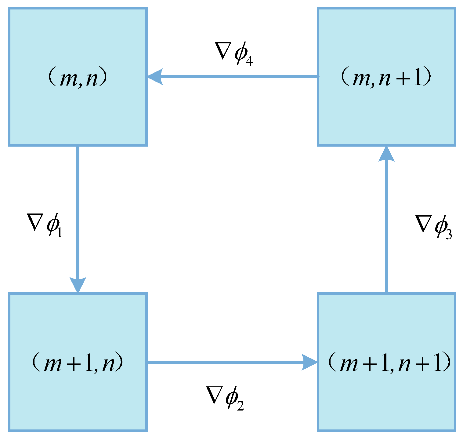
NOR can reflect the capacity to suppress noise of the filtering method. The smaller the NOR of the filtered interferometric phase, the stronger the capacity to suppress noise. The definition of residues depends on the loop integration of the phase gradient of neighboring pixels. For an interferometric phase image, the phase gradient between adjacent pixels can be obtained by
where and is the interferometric phase of adjacent pixel p and pixel , respectively. As shown in Figure 8, given a pixel , whether this point is a residue can be determined by
There are three possible values for F, namely 0 and , which correspond to a non-residue, a positive residue, and a negative residue, respectively. After judging each pixel in an interferometric phase image, its NOR can be obtained.
MSE is an index for measuring the difference between the filtered and clean interferometric phase. The smaller MSE means that the filtered interferometric phase is closer to the clean interferometric phase, but it does not consider the correlation between pixels in images. Therefore, MSSIM is employed to evaluate the structural similarity of the filtered and clean images. A higher MSSIM means that the structural information is kept better during the filtering process. For a clean interferometric phase patch x and the corresponding filtered patch y, the SSIM can be expressed as
where , , ,, are the local means, standard deviations and cross-covariance, and are constants and used to avoid instability when or is very close to zero, L is the dynamic range of the pixel values, and and are both small constants [48]. In order to evaluate the overall filtering quality of a filtered image, the MSSIM is adopted and it can be expressed as
where K is the number of patches, and and are the i-th patch in a clear interferometric phase image and the corresponding filtered image, respectively.
For real InSAR data, the no-reference metric Q is adopted, because the clean/reference interferometric phase is usually unknown. The index can comprehensively reflect the capacities of noise suppression and detail preservation of the filtering method [16,49], so it is suitable for our evaluation. According to [49], the local dominant orientation is calculated by the singular value decomposition of local interferometric phase image gradient matrix
where is the dominant orientation of the gradient field and is orthogonal to . are the singular values that represent the energy of phase gradient in the directions and , respectively. According to the singular values, the metric Q can be defined as
For a clean interferometric phase region, R is near 1, because is much larger than . When there is noise, R would decrease due to the destruction of the structure of this region. Therefore, a higher Q means that the accuracy of the filtering method is better.
4. Results and Discussion
We carry out a series of experiments on simulated and real data and compare our proposed method with the Lee filter, Goldstein filter, and InSAR-BM3D filter under the same experimental conditions in order to verify the effectiveness and robustness of the proposed method. For a clear comparison, qualitative and quantitative indexes are used for performance evaluation. All of the experiments were implemented on a PC with an i9-9900k CPU and an NVIDIA GeForce GTX 2080Ti GPU, and our proposed method is implemented on TensorFlow platform based on Python 3.6.6.
4.1. Experiments on Simulated Data
The data set was generated while using the simulated method that is described in Section 3.1. The size of the initial Gaussian distributed random matrix, the range of the unwrapped phase and the level of added noise are set to , 0–20 rad and −1.49 dB, respectively. The training set contains 10,000 pairs of real part images and 10,000 pairs of imaginary part images, and the testing set contains additional 2500 pairs of real part images and 2500 imaginary part images. We use Adam optimizer with a mini-batch size of 10 [41] and Glorot’s method [50] to initialized all trainable variables. The learning rate is exponentially decayed from an initial value of 1 to 0 with a power of 0.3. Early Stopping [51,52] is used to choose when to stop iteration, and 120,000 iterations are enough for convergence in our experiment that takes about six hours. In each iteration, the input training samples are randomly selected. After training, the trained PFNet was tested by the testing samples. We first randomly select a testing sample in order to visually analyze the filtering performance and then calculate the average evaluation indexes of all testing samples for quantitative analysis.
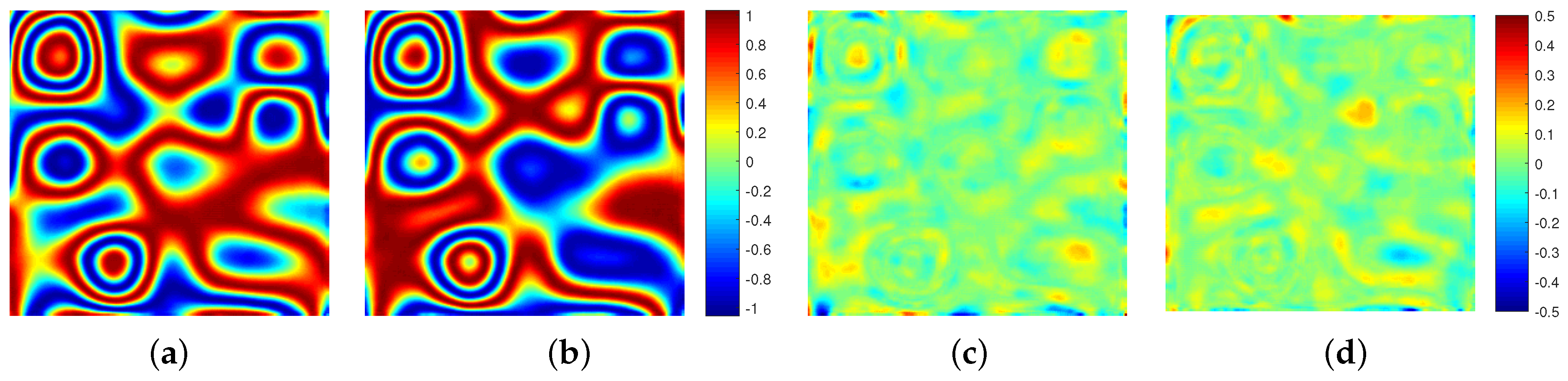
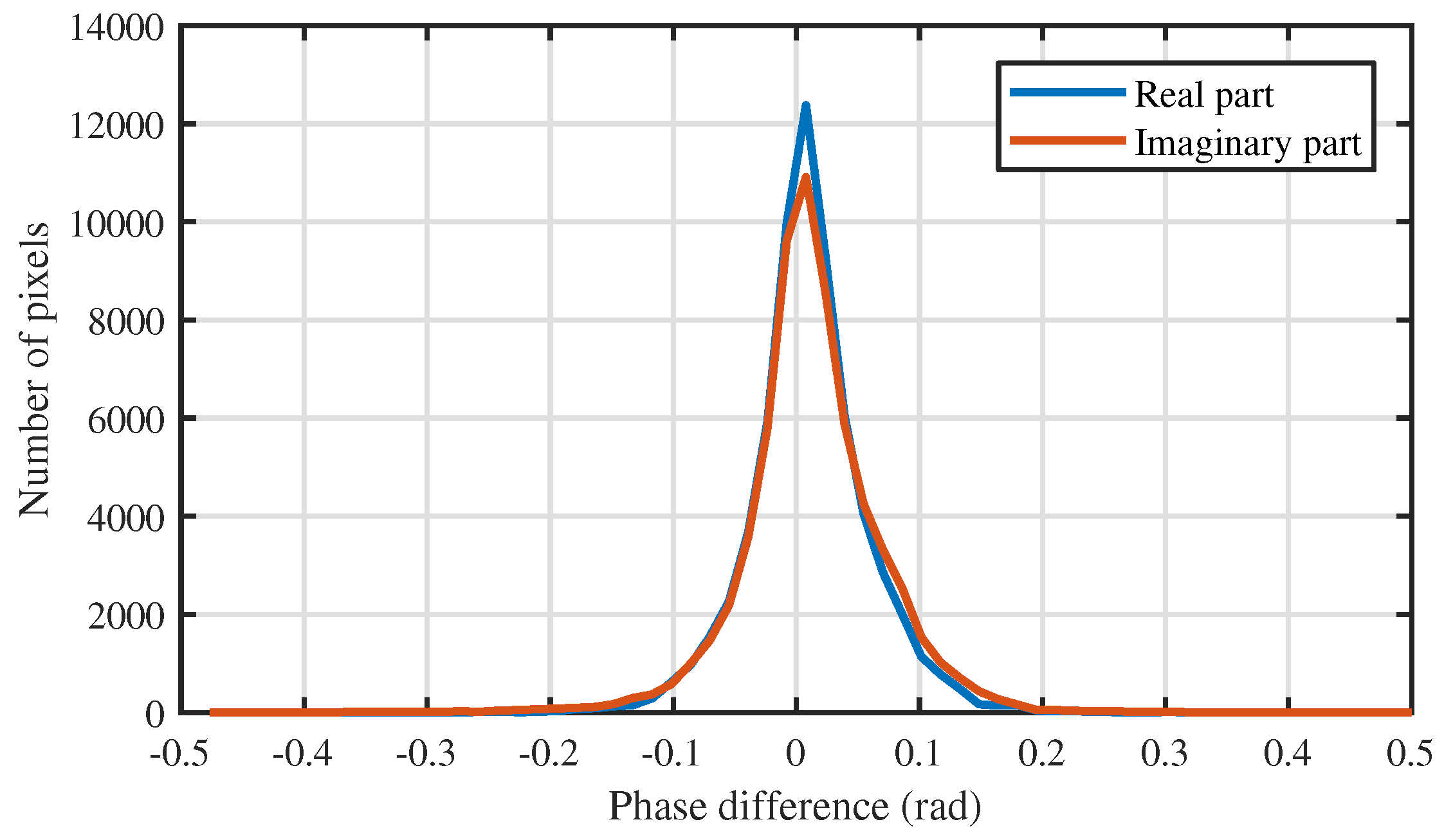
A clean interferometric phase image and its real part and imaginary part images are shown in Figure 9a–c, respectively. After noise is added, the corresponding noisy interferometric phase image and its real part and imaginary part images are shown in Figure 9d–f, respectively. The noisy real part and imaginary part images are filtered using the trained PFNet, and the filtered versions and the phase differences between the filtered version and the clean version are shown in Figure 10. We can observe that the filtered real part and imaginary part images are very close to the corresponding clean real part and imaginary part images, because most of the pixels of the phase difference images are close to zero. In order to more intuitively and clearly show this phase difference, the fitted histogram curves of the phase differences are shown in Figure 11. The histogram curve is plotted according to the value of the phase difference histogram, which reflects the distribution density of the phase difference. The vertical axis is the number of pixels and the horizontal axis is the value of the phase difference. From Figure 11, it can be seen that the two curves are sharp near zero, which indicates that the differences are small and concentrated near zero, that is, the noise is well suppressed in the real and imaginary parts of the noisy interferometric phase. According to the filtered real and imaginary parts, the filtered interferometric phase can be obtained using Equation (6).
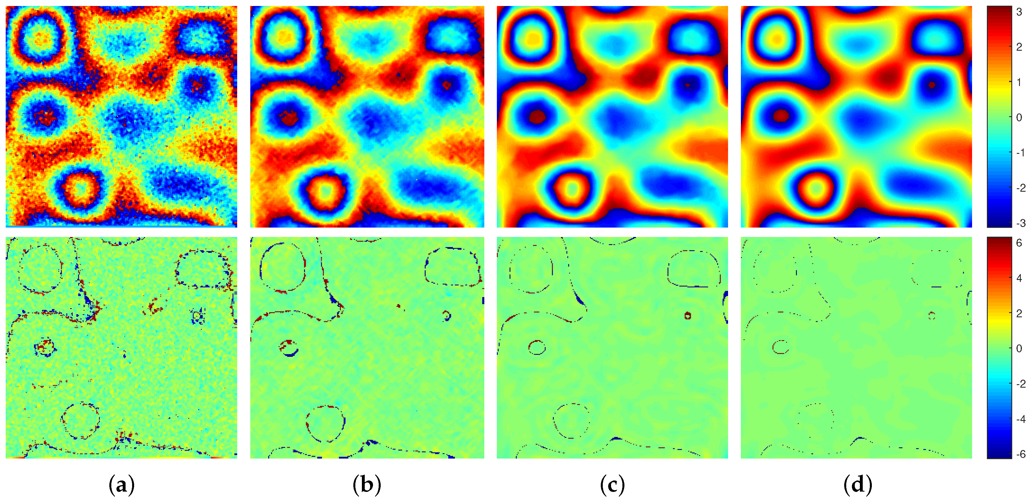
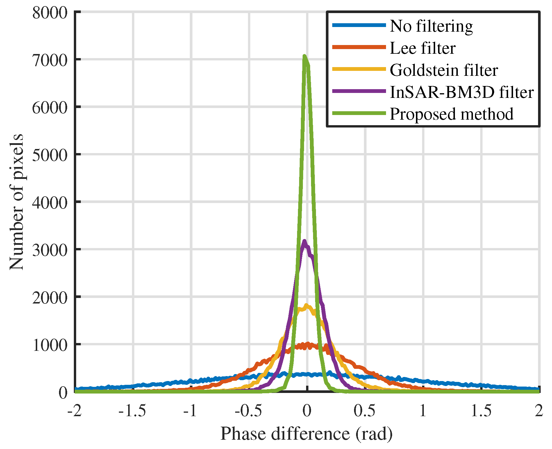
We compare our proposed method with three widely-used methods in order to further analyze the performance of the proposed method: the Lee filter, Goldstein filter, and InSAR-BM3D filter. Figure 12 shows the filtered interferometric phase images and the phase difference between the clean phase and filtered phase. We can see that the result of the proposed method is very close to the clean interferometric phase and is better than the other three methods from the naked eye, because its phase difference image is closer to zero. In order to more intuitively and clearly show this phase difference, the fitted histogram curves of the phase differences are shown in Figure 13. We can see that the fitted curve of the proposed method is sharper near zero than that of other methods, which indicates that the phase difference of the proposed method is more centered on zero, that is, the proposed method is significantly better from the perspective of the phase difference. Furthermore, the four aforementioned evaluation indexes, namely NOR, MSSIM, MSE, and T, are adopted and listed in Table 2. We can see that the proposed method obtains the lowest NOR and MSE, and the highest MSSIM, which reveals that the proposed method filters out the most noise and maintains the most detailed information among the four methods, which is, the proposed method has the strongest noise suppression capacity and the detail preservation capacity. In more detail, when compared with the InSAR-BM3D filter, the MSSIM and MSE of the proposed method are improved by 19.62% and 51.15%. Meanwhile, the proposed method has the smallest runtime (T), which means that it has a great advantage in computational efficiency. From another perspective, the proposed method has the highest accuracy, because the comprehensive evaluation of MSSIM and MSE reflects the accuracy of phase filtering. Combining accuracy and computational efficiency to analyze, we note that, although the runtime of the Lee filter and the Goldstein filter are less than the InSAR-BM3D filter, their MSSIM and MSE is not as good as the InSAR-BM3D filter. This contradiction between accuracy and computational efficiency has been resolved in the proposed method, because the runtime of the proposed method is the smallest and its accuracy is highest among the four methods. In summary, the proposed method is superior to the other three methods from qualitative and quantitative perspectives.
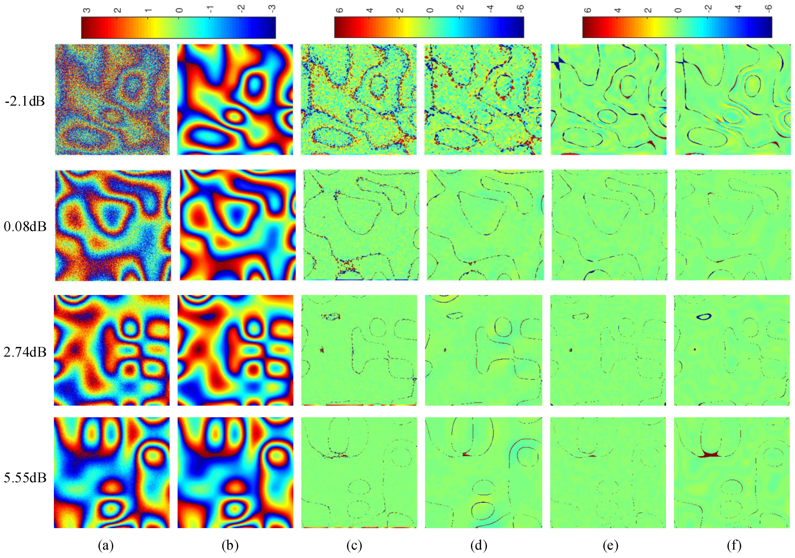
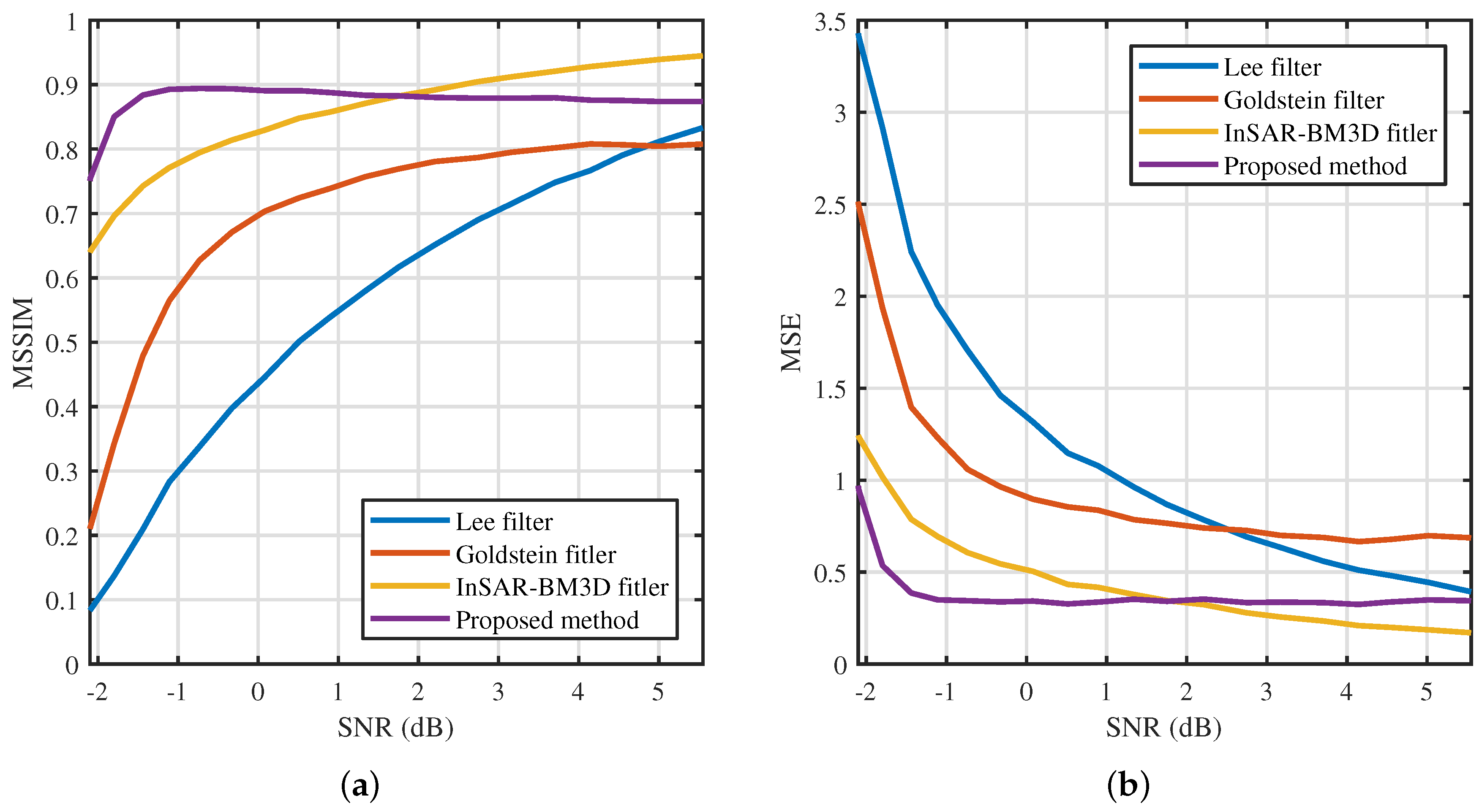
In the above experiments, the SNR of all testing samples is the same as the training samples, but, in practical applications, the SNR of the testing sample may be different from the training sample. Therefore, we next analyze the robustness of the proposed method when processing images with different values of SNR. We select four situations covering the range of noise from strong to weak for visual display, and the filtered results of four methods are shown in Figure 14. It can be seen that the proposed method and InSAR-BM3D filter outperform the other two methods in these four cases because their phase difference is closer to zero. Furthermore, when the SNR (−2.1 dB, 0.08 dB) of the testing sample is close to that of the training sample (−1.49 dB), the proposed method outperforms the InSAR-BM3D filter, and when the SNR (2.74 dB, 5.55 dB) of the testing sample is far from that of the training sample, the performance of the InSAR-BM3D filter is better than the proposed method. In order to quantitatively analyze the above-mentioned inferences, we calculated the MSSIM and MSE of each method according to the filtered results in the SNR range of (−2.1, 5.55) dB, as shown in Figure 15. It can be seen that the MSSIM of the proposed method and the InSAR-BM3D filter is significantly higher than the other two methods, and their MSE is significantly lower than the other two methods, which indicates that the capacities of noise suppression and detail preservation of the proposed method and InSAR-BM3D filter are significantly better. Next, comparing the proposed method with the InSAR-BM3D filter, the proposed method is significantly better than the InSAR-BM3D filter when the SNR of the testing sample is close to that of the training sample, which reveals that as long as the SNR of the testing sample keeps within a certain interval with the that of the training sample, the proposed method can obtain better performance than the InSAR-BM3D filter. Moreover, it is worth noting that the difficulty of filtering is greatly reduced in the case of high SNR, and the performance of the filtering algorithm in the case of low SNR is more worthy of attention. This is also the reason for choosing a lower SNR of training samples.
We carry out four experiments under the same condition, and each experiment halves the number of training samples in order to test the impact of the sample reduction on the performance of the proposed method. Their MSSIM and MSE are calculated and listed in Table 3. From Table 2 and Table 3, we can find that as the number of training samples decreases, the performance of the proposed method decreases slightly, but it is still better than the other three methods. That is to say, the performance of the proposed method is still better than the other three methods when the number of training samples is reduced by eight times.
In order to further demonstrate the performance of the proposed method, we compare it with another deep learning filtering method (called DeepInSAR) [35]. For a fair comparison, the data set used in this paper is the same as the data set used in [35] in terms of the data simulation method and number of images. The code of the simulation method can be downloaded from https://github.com/Lucklyric/InSAR-Simulator. The training set contains 28,800 pairs of real part images of simulated interferometric phases and 28,800 pairs of imaginary part images of simulated interferometric phases with a size of , and the testing set contains additional 900 pairs of simulated real part images and 900 pairs of simulated imaginary part images with a size of . In this experiment, the proposed method converges after 345,600 iterations, and the filtered results are obtained by the testing process. For quantitative analysis, the MSSIM and Root Mean Square Error (RMSE) of DeepInSAR are taken from [35], and the indexes of the two methods are listed in Table 4. From Table 4, it can been seen that the MSSIM of the proposed method is comparable to DeepInSAR, and its RMSE is greatly improved by 21.47%. Therefore, the overall performance the proposed method is better than DeepInSAR on the same data set.
4.2. Experiments on Real Data
In this section, we use the training samples that were generated by the real DEM to train the proposed network. The detailed sample generation process is described in Section 3.1. The learning rate and mini-batch size are the same as in Section 4.1, and 31,600 iterations are enough for convergence. After training, two interferograms (SIR-C/X-SAR data and TerraSAR-X data) are processed in order to evaluate the performance and generalization ability of the proposed method.
4.2.1. SIR-C/X-SAR Data
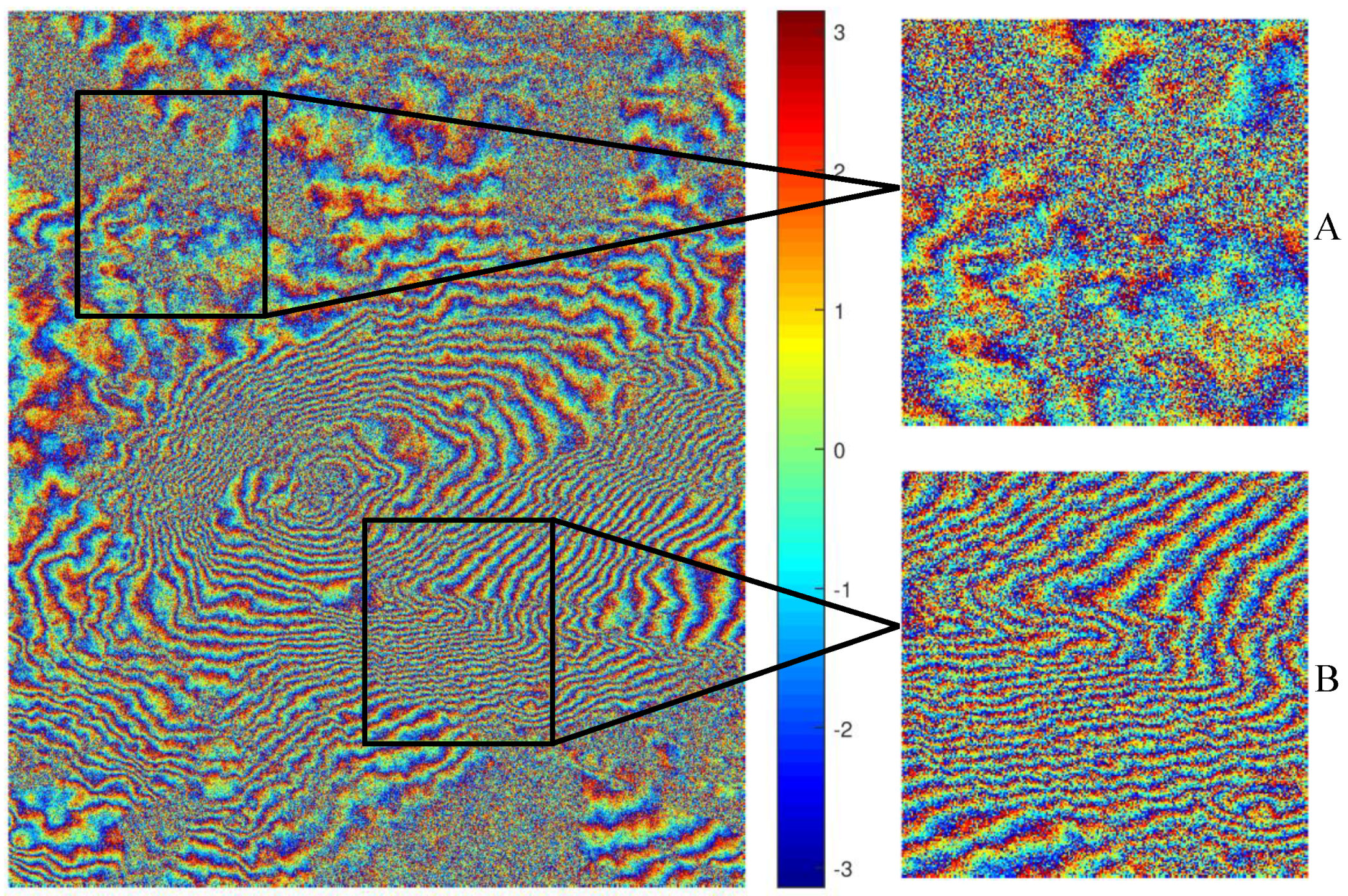
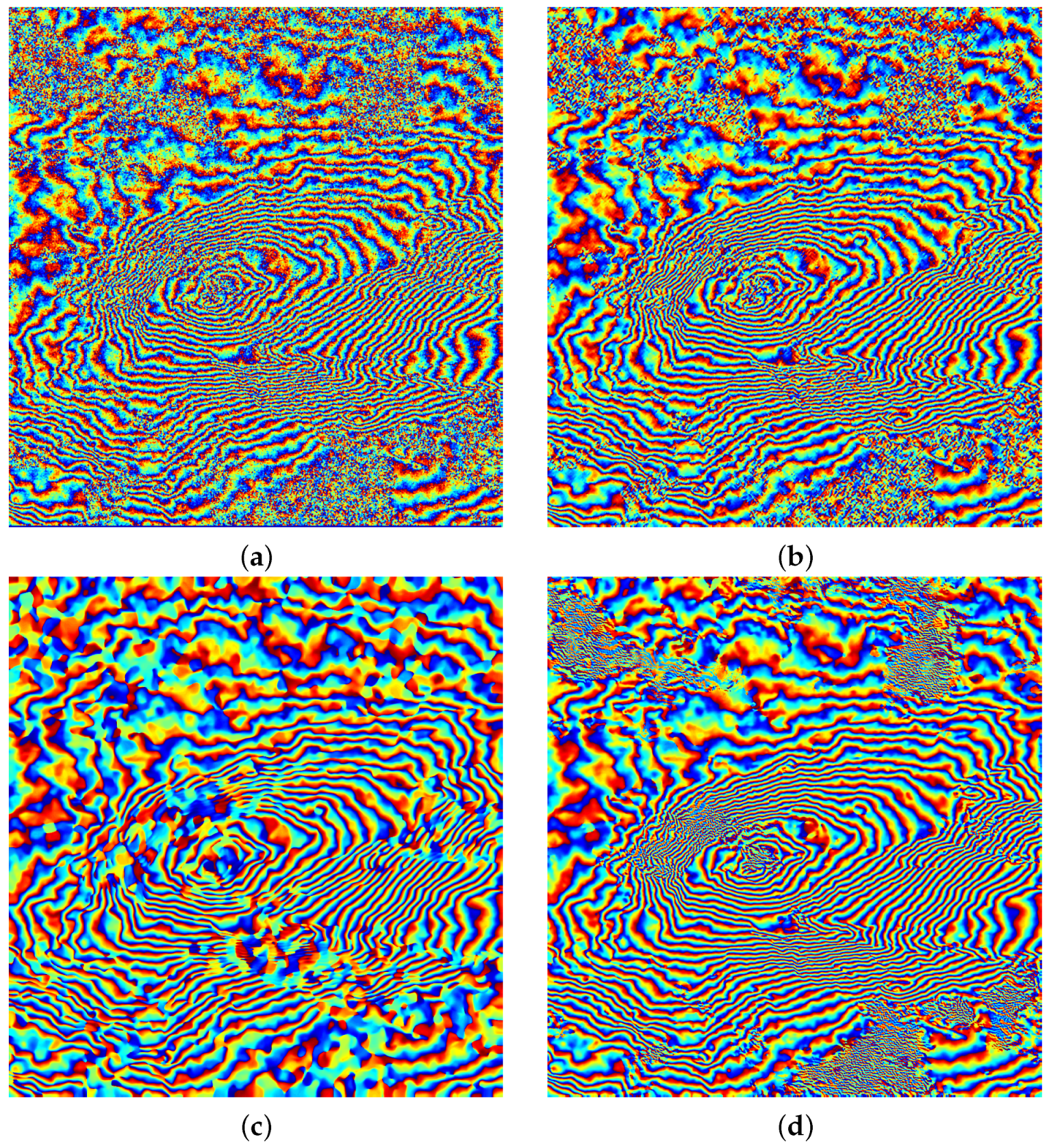
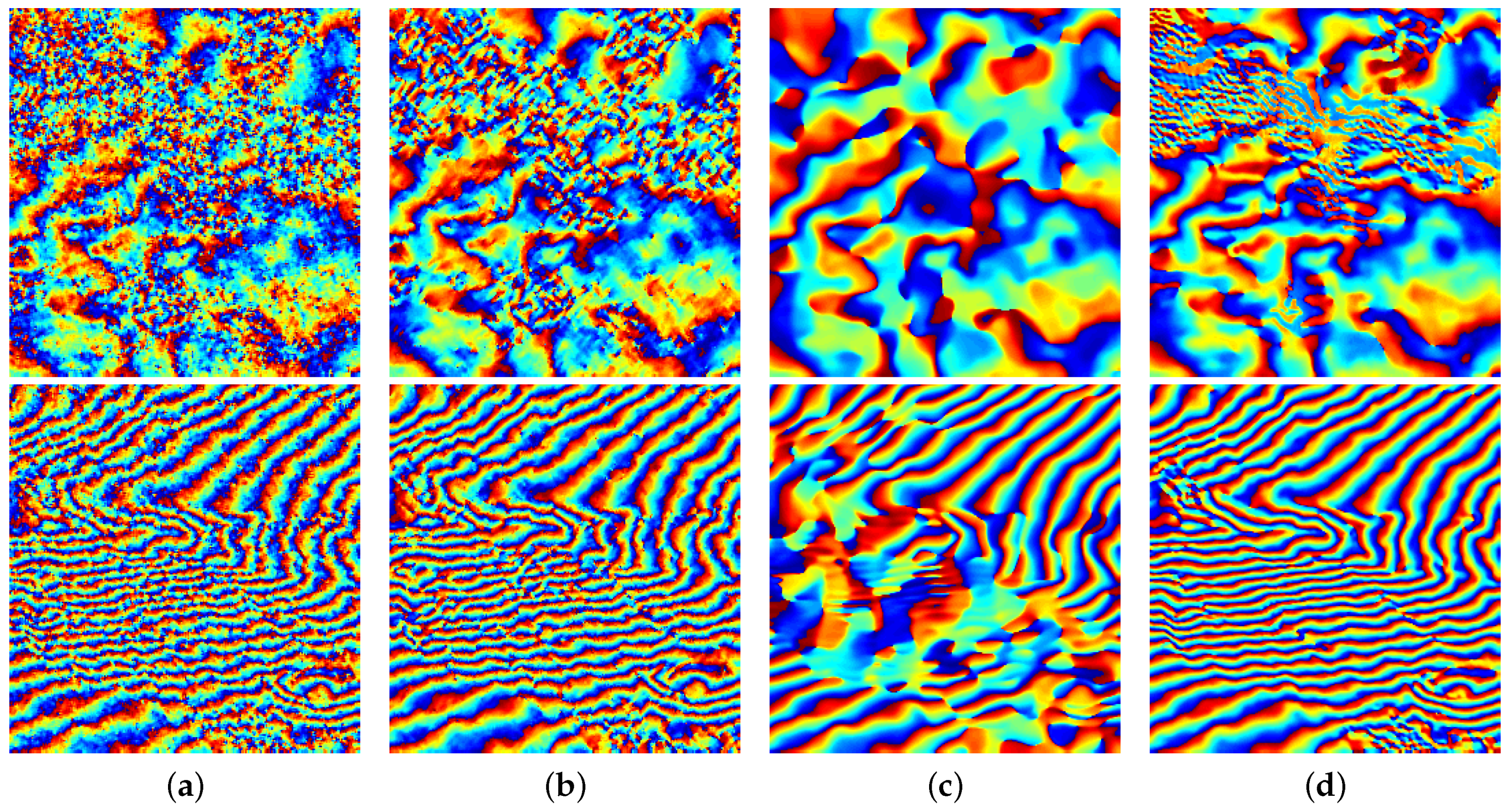
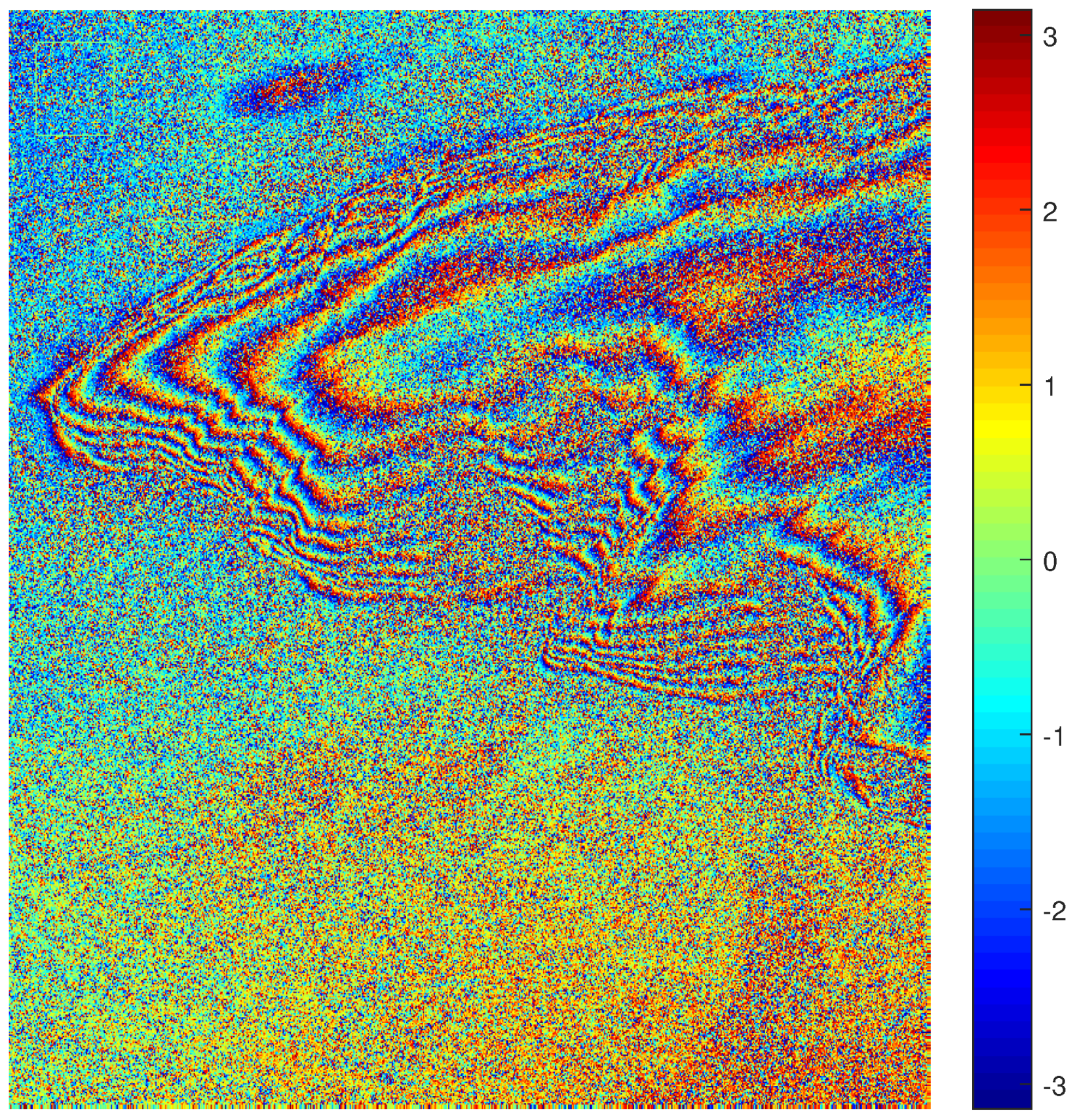
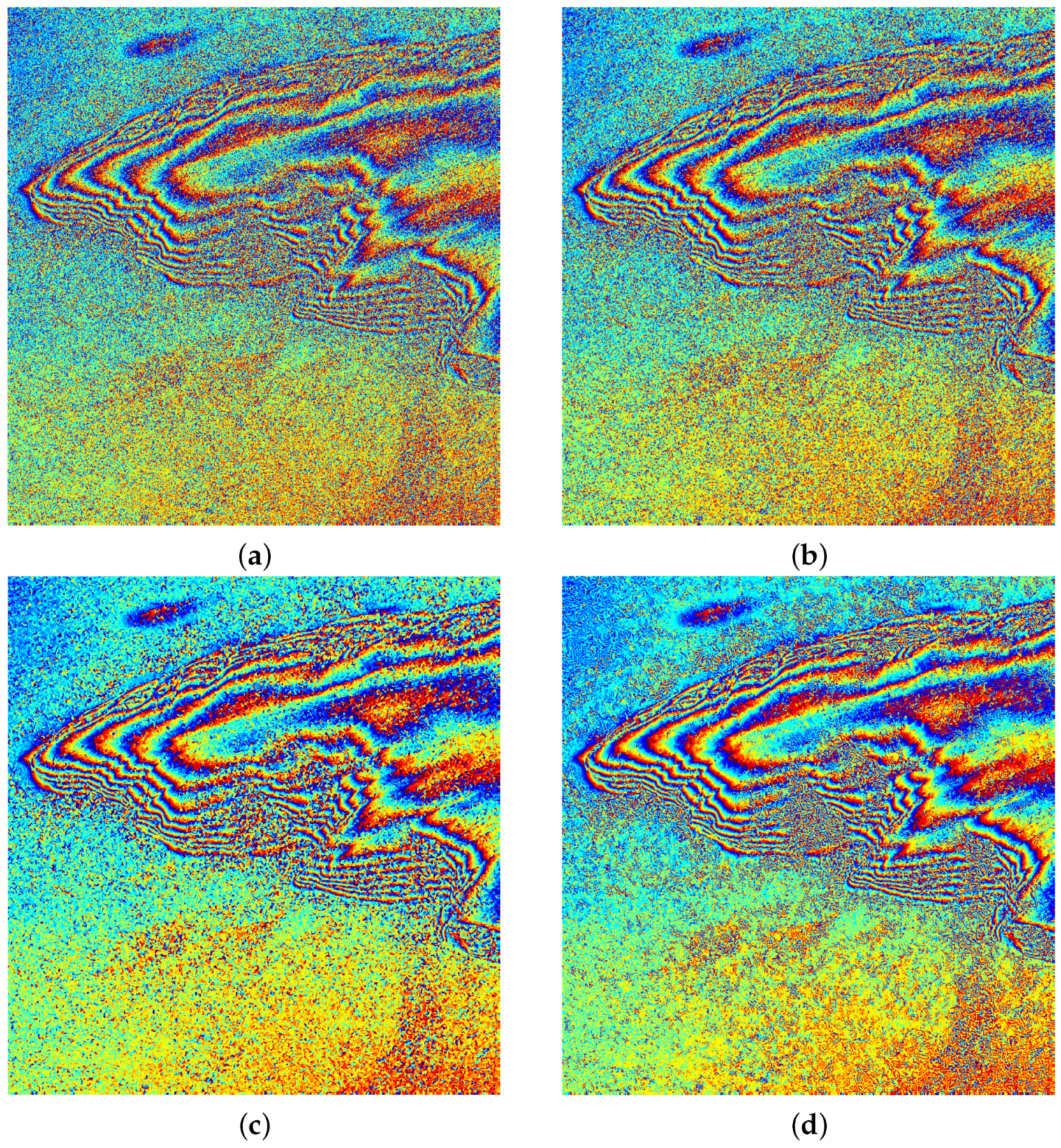
In this subsection, a real interferometric phase image with a size of pixels (SIR-C/X-SAR, Etna Volcano, Italy) was used as a testing sample, as shown in Figure 16. The interferogram was obtained from two SLC images acquired by two shuttle passes on 9 and 10 October 1994 [53], and no multilook processing was performed. For a better comparison of the detailed filtering effects of areas with different values of coherence, a low coherence area (labeled A) and a high coherence area ( labeled B) are enlarged in Figure 16. For qualitative evaluation, the filtered results of Figure 16 using the Lee filter, Goldstein filter, InSAR-BM3D filter, and the proposed method are shown in Figure 17 and Figure 18. From these two figures, we can infer that the results of the Lee filter and Goldstein filter preserve more noise, which is, the noise suppression capacity is not enough, while the result of InSAR-BM3D smooths the fringe edges excessively, that is, the detail preservation capacity is insufficient. Note that the filtering result of the proposed method reaches a balance between the two states among the four methods.
To confirm the above-mentioned inference, the quantitative evaluation indexes of Figure 16 and the corresponding filtered results are calculated and listed in Table 5. Because the corresponding clean interferometric phase is unknown, MSE is no longer used, but the no-reference metric Q that can comprehensively reflect the capacities of noise suppression and detail preservation is used. In addition, due to the residues of Figure 16 can not completely be filtered, the percentage of the reduced residues (PRR) is also calculated to show the noise suppression capacity more clearly. From Table 5, we can see that the PRR and metric Q of the Lee filter and Goldstein filter are significantly lower than the InSAR-BM3D filter and proposed method. When comparing the latter two methods, although the InSAR-BM3D filter has a higher PRR, its Q is lower, which means that its noise suppression capacity is too strong and some detailed information is lost. In more detail, the metric Q of the proposed method increases by 70.76% as compared with the InSAR-BM3D filter. Therefore, it can be seen that the proposed method maintains the best balance between the two capacities among the four methods, which is consistent with the above-mentioned qualitative inference from images. In addition, although the InSAR-BM3D filter has higher MSSIM and PRR than the Lee filter and Goldstein filter, it consumes multiple runtime, which shows the same contradiction between accuracy and computational efficiency as in the simulation experiments. However, the runtime of the proposed method is only about 0.043 s while ensuring the best balance between the noise suppression capacity and detail preservation capacity among the four methods. When compared with the runtime of InSAR-BM3D filter (125.2 s), this thousand-fold improvement in computational efficiency has a great advantage in practical applications that require real-time processing.
4.2.2. TerraSAR-X Data
A real interferometric phase image with a size of pixels (TerraSAR-X, Uluru, Australia) was used as a testing sample in order to further evaluate the generalization ability of the proposed method on real InSAR data, as shown in Figure 19. The interferogram was obtained from two SLC images acquired by two satellite passes on 12 and 23 February 2009 [54], and no multilook processing was performed. The interferogram was processed by the proposed method as a whole. The filtered results are shown in Figure 20 and the quantitative indexes are listed in Table 6. From Figure 20 and Table 6, we can see that the PRR and metric Q of the Lee filter and Goldstein filter are lower than the InSAR-BM3D filter and proposed method. When comparing the latter two methods, although the InSAR-BM3D filter has a higher PRR, its Q is lower, which means that it lost some detailed information due to its strong noise suppression capacity. In more detail, the metric Q of the proposed method increases by 14.84% as compared with the InSAR-BM3D filter. Therefore, it can be seen that the proposed method maintains the best balance between detail preservation and noise suppression among the four methods, which is consistent with the conclusion presented in Section 4.2.1. Through the above analysis, it can be seen that the performance of the proposed method is still better than the other three methods, which further verifies its generalization ability. In addition, comparing the runtime of the InSAR-BM3D filter and the proposed method, the efficiency advantage of the proposed method has been verified again.
5. Conclusions
An interferometric phase filtering method based on deep learning is proposed in this paper in order to better balance the noise suppression capacity and the phase detail preservation capacity and ensure computational efficiency when compared with the widely-used phase filtering methods. In this method, PFNet is used to filter the real and imaginary parts of the interferometric phase. With a scale recurrent strategy, the network includes three single scale subnetworks based on the encoder-decoder architecture. Because the three subnetworks are connected by RNN units that can transmit current state information among different subnetworks, the method can utilize the global structural phase information contained in the different-scaled feature maps. The encoder part is used for extracting the phase features, and the decoder part restores detailed information from the encoded feature maps and makes the size of the output image the same as that of the input image. Experiments on simulated and real InSAR data prove that the proposed method is superior to three widely-used phase filtering methods by qualitative and quantitative comparisons. When compared with the InSAR-BM3D filter, MSSIM and MSE of the proposed method in simulation experiments are improved by 19.62% and 51.15%. In addition, when the SNR of the testing sample is close to the SNR of the training sample, the proposed method can obtain better performance. When the number of training samples is reduced by eight times, the performance of the proposed method is still better than the other three methods. Moreover, on the same data set, the overall performance the proposed method is better than DeepInSAR, because the MSSIM of the proposed method is comparable to DeeInSAR, while its RMSE is improved by 21.47%. When processing SIR-C/X-SAR data, the metric Q of the proposed method increases by 70.76% as compared with the InSAR-BM3D filter, and the runtime of the proposed method is only about 0.043 s for a real interferometric image with a size of pixels, which has the significant advantage of computational efficiency in practical applications that require real-time processing. Furthermore, when processing TerraSAR-X data without retraining, the metric Q of the proposed method increases by 14.84% compared with the InSAR-BM3D filter, which further verifies the generalization ability of the proposed method.
The proposed method successfully introduces scale recurrent networks into the field of InSAR phase filtering. This suggests a path for future research that may focus on new networks with the capacity for better detail preservation and noise suppression. A second topic of future work will be to apply the proposed method to more real data sets.
Author Contributions
All authors made significant contributions to the work. L.P., X.Z., Z.Z. and J.S. designed the research and analyzed the results. L.P. and Z.Z. performed the experiments. L.P. and X.Z. wrote and revised the manuscript. S.W. and Y.Z. provided suggestions for the preparation and revision of the paper. All authors have read and agreed to the published version of the manuscript.
Funding
This work was supported in part by the National Key R&D Program of China under Grant 2017YFB0502700 and in part by the National Natural Science Foundation of China under Grants 61571099, 61501098, and 61671113.
Acknowledgments
We thank all the reviewers and editors for their comments towards improving this manuscript.
Conflicts of Interest
The authors declare no conflict of interest.
References
- Moreira, A.; Prats-Iraola, P.; Younis, M.; Krieger, G.; Hajnsek, I.; Papathanassiou, K.P. A tutorial on synthetic aperture radar. IEEE Geosci. Remote Sens. Mag. 2013, 1, 6–43. [Google Scholar] [CrossRef] [Green Version]
- Zhu, X.; Wang, Y.; Montazeri, S.; Ge, N. A Review of Ten-Year Advances of Multi-Baseline SAR Interferometry Using TerraSAR-X Data. Remote Sens. 2018, 10, 1374. [Google Scholar] [CrossRef] [Green Version]
- Wang, Y.; Huang, H.; Dong, Z.; Wu, M. Modified patch-based locally optimal Wiener method for interferometric SAR phase filtering. ISPRS J. Photogramm. Remote Sens. 2016, 114, 10–23. [Google Scholar] [CrossRef] [Green Version]
- Lee, J.S.; Papathanassiou, K.P.; Ainsworth, T.L.; Grunes, M.R.; Reigber, A. A new technique for noise filtering of SAR interferometric phase images. IEEE Trans. Geosci. Remote Sens. 1998, 36, 1456–1465. [Google Scholar]
- Vasile, G.; Trouvé, E.; Lee, J.S.; Buzuloiu, V. Intensity-driven adaptive-neighborhood technique for polarimetric and interferometric SAR parameters estimation. IEEE Trans. Geosci. Remote Sens. 2006, 44, 1609–1621. [Google Scholar] [CrossRef] [Green Version]
- Fu, S.; Long, X.; Yang, X.; Yu, Q. Directionally adaptive filter for synthetic aperture radar interferometric phase images. IEEE Trans. Geosci. Remote Sens. 2012, 51, 552–559. [Google Scholar] [CrossRef]
- Chao, C.F.; Chen, K.S.; Lee, J.S. Refined filtering of interferometric phase from InSAR data. IEEE Trans. Geosci. Remote Sens. 2013, 51, 5315–5323. [Google Scholar] [CrossRef]
- Yu, Q.; Yang, X.; Fu, S.; Liu, X.; Sun, X. An adaptive contoured window filter for interferometric synthetic aperture radar. IEEE Geosci. Remote Sens. Lett. 2007, 4, 23–26. [Google Scholar] [CrossRef]
- Goldstein, R.M.; Werner, C.L. Radar interferogram filtering for geophysical applications. Geophys. Res. Lett. 1998, 25, 4035–4038. [Google Scholar] [CrossRef] [Green Version]
- Baran, I.; Stewart, M.P.; Kampes, B.M.; Perski, Z.; Lilly, P. A modification to the Goldstein radar interferogram filter. IEEE Trans. Geosci. Remote Sens. 2003, 41, 2114–2118. [Google Scholar] [CrossRef] [Green Version]
- Trouve, E.; Nicolas, J.M.; Maitre, H. Improving phase unwrapping techniques by the use of local frequency estimates. IEEE Trans. Geosci. Remote Sens. 1998, 36, 1963–1972. [Google Scholar] [CrossRef] [Green Version]
- Song, R.; Guo, H.; Liu, G.; Perski, Z.; Fan, J. Improved Goldstein SAR interferogram filter based on empirical mode decomposition. IEEE Geosci. Remote Sens. Lett. 2013, 11, 399–403. [Google Scholar] [CrossRef]
- Abdallah, W.B.; Abdelfattah, R. Two-dimensional wavelet algorithm for interferometric synthetic aperture radar phase filtering enhancement. J. Appl. Remote Sens. 2015, 9, 096061. [Google Scholar] [CrossRef]
- Lopez-Martinez, C.; Fabregas, X. Modeling and reduction of SAR interferometric phase noise in the wavelet domain. IEEE Trans. Geosci. Remote Sens. 2002, 40, 2553–2566. [Google Scholar] [CrossRef] [Green Version]
- Zha, X.; Fu, R.; Dai, Z.; Liu, B. Noise reduction in interferograms using the wavelet packet transform and wiener filtering. IEEE Geosci. Remote Sens. Lett. 2008, 5, 404–408. [Google Scholar]
- Fang, D.; Lv, X.; Wang, Y.; Lin, X.; Qian, J. A sparsity-based InSAR phase denoising algorithm using nonlocal wavelet shrinkage. Remote Sens. 2016, 8, 830. [Google Scholar] [CrossRef] [Green Version]
- Buades, A.; Coll, B.; Morel, J.M. A review of image denoising algorithms, with a new one. Multiscale Model. Simul. 2005, 4, 490–530. [Google Scholar] [CrossRef]
- Parrilli, S.; Poderico, M.; Angelino, C.V.; Verdoliva, L. A nonlocal SAR image denoising algorithm based on LLMMSE wavelet shrinkage. IEEE Trans. Geosci. Remote Sens. 2011, 50, 606–616. [Google Scholar] [CrossRef]
- Cozzolino, D.; Parrilli, S.; Scarpa, G.; Poggi, G.; Verdoliva, L. Fast adaptive nonlocal SAR despeckling. IEEE Geosci. Remote Sens. Lett. 2013, 11, 524–528. [Google Scholar] [CrossRef] [Green Version]
- Deledalle, C.A.; Denis, L.; Tupin, F. NL-InSAR: Nonlocal interferogram estimation. IEEE Trans. Geosci. Remote Sens. 2010, 49, 1441–1452. [Google Scholar] [CrossRef]
- Chen, R.; Yu, W.; Wang, R.; Liu, G.; Shao, Y. Interferometric phase denoising by pyramid nonlocal means filter. IEEE Geosci. Remote Sens. Lett. 2013, 10, 826–830. [Google Scholar] [CrossRef]
- Lin, X.; Li, F.; Meng, D.; Hu, D.; Ding, C. Nonlocal SAR interferometric phase filtering through higher order singular value decomposition. IEEE Geosci. Remote Sens. Lett. 2014, 12, 806–810. [Google Scholar] [CrossRef]
- Su, X.; Deledalle, C.A.; Tupin, F.; Sun, H. Two-step multitemporal nonlocal means for synthetic aperture radar images. IEEE Trans. Geosci. Remote Sens. 2014, 52, 6181–6196. [Google Scholar]
- Sica, F.; Reale, D.; Poggi, G.; Verdoliva, L.; Fornaro, G. Nonlocal adaptive multilooking in SAR multipass differential interferometry. IEEE J. Sel. Top. Appl. Earth Obs. Remote Sens. 2015, 8, 1727–1742. [Google Scholar] [CrossRef] [Green Version]
- Baier, G.; Rossi, C.; Lachaise, M.; Zhu, X.X.; Bamler, R. A Nonlocal InSAR Filter for High-Resolution DEM Generation From TanDEM-X Interferograms. IEEE Trans. Geosci. Remote Sens. 2018, 56, 6469–6483. [Google Scholar] [CrossRef] [Green Version]
- Sica, F.; Cozzolino, D.; Zhu, X.X.; Verdoliva, L.; Poggi, G. INSAR-BM3D: A nonlocal filter for SAR interferometric phase restoration. IEEE Trans. Geosci. Remote Sens. 2018, 56, 3456–3467. [Google Scholar] [CrossRef] [Green Version]
- Tao, X.; Gao, H.; Shen, X.; Wang, J.; Jia, J. Scale-recurrent network for deep image deblurring. In Proceedings of the IEEE Conference on Computer Vision and Pattern Recognition, Salt Lake City, UT, USA, 18–23 June 2018; pp. 174–8182. [Google Scholar]
- Ronneberger, O.; Fischer, P.; Brox, T. U-net: Convolutional networks for biomedical image segmentation. In Proceedings of the International Conference on Medical Image Computing and Computer-Assisted Intervention, Munich, Germany, 5–9 October 2015; Springer: Cham, Switzerland, 2015; pp. 234–241. [Google Scholar]
- Nah, S.; Hyun Kim, T.; Mu Lee, K. Deep multi-scale convolutional neural network for dynamic scene deblurring. In Proceedings of the IEEE Conference on Computer Vision and Pattern Recognition, Honolulu, HI, USA, 21–26 July 2017; pp. 3883–3891. [Google Scholar]
- Hirose, A. Complex-Valued Neural Networks; Springer Science & Business Media: Berlin/Heidelberg, Germany, 2012; Volume 400. [Google Scholar]
- Wang, P.; Zhang, H.; Patel, V.M. SAR image despeckling using a convolutional neural network. IEEE Signal Process. Lett. 2017, 24, 1763–1767. [Google Scholar] [CrossRef] [Green Version]
- Zhou, Y.; Shi, J.; Yang, X.; Wang, C.; Kumar, D.; Wei, S.; Zhang, X. Deep multi-scale recurrent network for synthetic aperture radar images despeckling. Remote Sens. 2019, 11, 2462. [Google Scholar] [CrossRef] [Green Version]
- Zhang, Q.; Yuan, Q.; Li, J.; Yang, Z.; Ma, X. Learning a dilated residual network for SAR image despeckling. Remote Sens. 2018, 10, 196. [Google Scholar] [CrossRef] [Green Version]
- Mukherjee, S.; Zimmer, A.; Kottayil, N.K.; Sun, X.; Ghuman, P.; Cheng, I. CNN-Based InSAR Denoising and Coherence Metric. In Proceedings of the 2018 IEEE SENSORS, New Delhi, India, 28–31 October 2018; pp. 1–4. [Google Scholar]
- Sun, X.; Zimmer, A.; Mukherjee, S.; Kottayil, N.K.; Ghuman, P.; Cheng, I. DeepInSAR—A Deep Learning Framework for SAR Interferometric Phase Restoration and Coherence Estimation. Remote Sens. 2020, 12, 2340. [Google Scholar] [CrossRef]
- Anantrasirichai, N.; Biggs, J.; Albino, F.; Hill, P.; Bull, D. Application of machine learning to classification of volcanic deformation in routinely generated InSAR data. J. Geophys. Res. Solid Earth 2018, 123, 6592–6606. [Google Scholar] [CrossRef] [Green Version]
- Bamler, R.; Hartl, P. Synthetic aperture radar interferometry. Inverse Probl. 1998, 14, R1. [Google Scholar] [CrossRef]
- Rosen, P.A.; Hensley, S.; Joughin, I.R.; Li, F.K.; Madsen, S.N.; Rodriguez, E.; Goldstein, R.M. Synthetic aperture radar interferometry. Proc. IEEE 2000, 88, 333–382. [Google Scholar] [CrossRef]
- Wang, K.; Li, Y.; Kemao, Q.; Di, J.; Zhao, J. One-step robust deep learning phase unwrapping. Opt. Express 2019, 27, 15100–15115. [Google Scholar] [CrossRef]
- Zhou, L.; Yu, H.; Lan, Y. Deep Convolutional Neural Network-Based Robust Phase Gradient Estimation for Two-Dimensional Phase Unwrapping Using SAR Interferograms. IEEE Trans. Geosci. Remote. Sens. 2020, 58, 4653–4665. [Google Scholar] [CrossRef]
- Kingma, D.P.; Ba, J. Adam: A method for stochastic optimization. arXiv 2014, arXiv:1412.6980. [Google Scholar]
- Hochreiter, S.; Schmidhuber, J. Long short-term memory. Neural Comput. 1997, 9, 1735–1780. [Google Scholar] [CrossRef]
- Chung, J.; Gulcehre, C.; Cho, K.; Bengio, Y. Empirical evaluation of gated recurrent neural networks on sequence modeling. arXiv 2014, arXiv:1412.3555. [Google Scholar]
- Lei, T.; Zhang, Y.; Wang, S.I.; Dai, H.; Artzi, Y. Simple recurrent units for highly parallelizable recurrence. arXiv 2017, arXiv:1709.02755. [Google Scholar]
- Matthew, D.; Fergus, R. Visualizing and understanding convolutional neural networks. In Proceedings of the 13th European Conference Computer Vision and Pattern Recognition, Zurich, Switzerland, 6–12 September 2014; pp. 6–12. [Google Scholar]
- He, K.; Zhang, X.; Ren, S.; Sun, J. Deep residual learning for image recognition. In Proceedings of the IEEE Conference on Computer Vision and Pattern Recognition, Las Vegas, NV, USA, 27–30 June 2016; pp. 770–778. [Google Scholar]
- Mao, X.; Shen, C.; Yang, Y.B. Image restoration using very deep convolutional encoder-decoder networks with symmetric skip connections. In Proceedings of the 30th Conference on Neural Information Processing Systems, Barcelona, Spain, 5–10 December 2016; pp. 2802–2810. [Google Scholar]
- Wang, Z.; Bovik, A.C.; Sheikh, H.R.; Simoncelli, E.P. Image quality assessment: From error visibility to structural similarity. IEEE Trans. Image Process. 2004, 13, 600–612. [Google Scholar] [CrossRef] [Green Version]
- Zhu, X.; Milanfar, P. Automatic Parameter Selection for Denoising Algorithms Using a No-Reference Measure of Image Content. IEEE Trans. Image Process. 2010, 19, 3116–3132. [Google Scholar]
- Glorot, X.; Bengio, Y. Understanding the difficulty of training deep feedforward neural networks. In Proceedings of the Thirteenth International Conference on Artificial Intelligence and Statistics, Chia Laguna Resort, Sardinia, Italy, 13–15 May 2010; pp. 249–256. [Google Scholar]
- Yao, Y.; Rosasco, L.; Caponnetto, A. On early stopping in gradient descent learning. Constr. Approx. 2007, 26, 289–315. [Google Scholar] [CrossRef]
- Raskutti, G.; Wainwright, M.J.; Yu, B. Early stopping and non-parametric regression: An optimal data-dependent stopping rule. J. Mach. Learn. Res. 2014, 15, 335–366. [Google Scholar]
- Coltelli, M.; Fornaro, G.; Franceschetti, G.; Lanari, R.; Migliaccio, M.; Moreira, J.R.; Papathanassiou, K.P.; Puglisi, G.; Riccio, D.; Schwabisch, M. On the survey of volcanic sites: The SIR-C/X-SAR interferometry. In Proceedings of the IGARSS’96, 1996 International Geoscience and Remote Sensing Symposium, Lincoln, NE, USA, 31–31 May 1996; Volume 1, pp. 350–352. [Google Scholar]
- Pitz, W.; Miller, D. The TerraSAR-X satellite. IEEE Trans. Geosci. Remote Sens. 2010, 48, 615–622. [Google Scholar] [CrossRef]
Figure 1.
InSAR geometry model.

Figure 2.
Two examples of the random matrices and the corresponding unwrapped phases and interferometric phases. (a) A random matrix (). (b,c) are the corresponding unwrapped phase and interferometric phase, respectively, when the range of the unwrapped phase is 0–20 rad. (d) A random matrix (). (e,f) are the corresponding unwrapped phase and interferometric phase respectively when the range of the unwrapped phase is 0–20 rad. (g,h) are the corresponding unwrapped phase and interferometric phase, respectively, when the range of the unwrapped phase is 0–30 rad.

Figure 3.
Interferometric phase images with different levels of noise. (a) 1.17 dB. (b) −0.87 dB. (c) −2.1 dB.
Figure 3.
Interferometric phase images with different levels of noise. (a) 1.17 dB. (b) −0.87 dB. (c) −2.1 dB.

Figure 4.
Two examples of using DEMs to generate samples. (a) Unwrapped phase (maximum is 150). (b,c) are the corresponding clean interferometric phase and noisy interferometric phase, respectively. (d) Unwrapped phase (maximum is 250). (e,f) are the corresponding clean interferometric phase and noisy interferometric phase, respectively.

Figure 5.
(a) Training and (b) testing process of the proposed method.

Figure 6.
Overall architecture of PFNet.

Figure 7.
Detailed structure of each subnetwork.

Figure 8.
Schematic diagram of residue calculation.

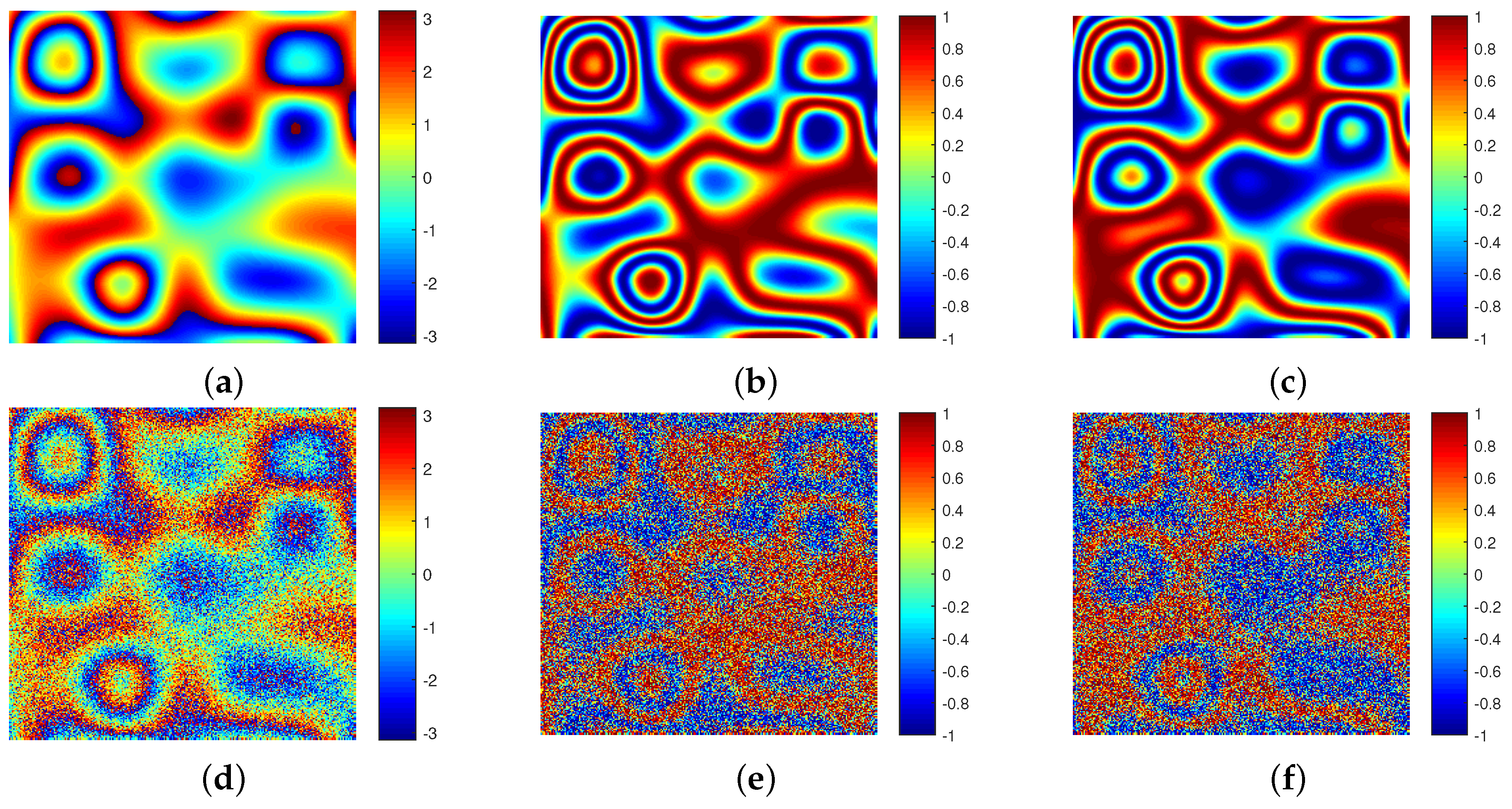
Figure 9.
Simulated interferometric phase. (a) Clean interferometric phase, and its (b) real part and (c) imaginary part. (d) Noisy version of (a), and its (e) real part and (f) imaginary part.
Figure 9.
Simulated interferometric phase. (a) Clean interferometric phase, and its (b) real part and (c) imaginary part. (d) Noisy version of (a), and its (e) real part and (f) imaginary part.

Figure 10.
Filtered results and phase differences of Figure 9e,f using PFNet. (a) Filtered result of the real part. (b) Filtered result of the imaginary part. (c) Phase difference of the real part. (d) Phase difference of the imaginary part.
Figure 10.
Filtered results and phase differences of Figure 9e,f using PFNet. (a) Filtered result of the real part. (b) Filtered result of the imaginary part. (c) Phase difference of the real part. (d) Phase difference of the imaginary part.

Figure 11.
Fitted phase difference histogram curves of Figure 10c,d.
Figure 11.
Fitted phase difference histogram curves of Figure 10c,d.

Figure 12.
Filtered results (Top) and phase difference (Bottom) of four methods on simulated data. (a) Lee filter. (b) Goldstein filter. (c) InSAR-BM3D filter. (d) Proposed method.
Figure 12.
Filtered results (Top) and phase difference (Bottom) of four methods on simulated data. (a) Lee filter. (b) Goldstein filter. (c) InSAR-BM3D filter. (d) Proposed method.

Figure 13.
Fitted phase difference histogram curves of four methods.

Figure 14.
Filtered results of four methods for images with different values of SNR. (a) Noisy interferometric phase. (b) Clean interferometric phase. (c) Phase difference of the Lee filter. (d) Phase difference of the Goldstein filter. (e) Phase difference of the InSAR-BM3D filter. (f) Phase difference of the proposed method.

Figure 15.
Quantitative indexes of four methods on simulated images with different values of signal-to-noise ratio (SNR). (a) Mean structural similarity index (MSSIM). (b) Mean-square error (MSE).
Figure 15.
Quantitative indexes of four methods on simulated images with different values of signal-to-noise ratio (SNR). (a) Mean structural similarity index (MSSIM). (b) Mean-square error (MSE).

Figure 16.
SIR-C/X-SAR data: a real interferometric phase image and its a low coherence area (labeled A) and a high coherence area (labeled B).
Figure 16.
SIR-C/X-SAR data: a real interferometric phase image and its a low coherence area (labeled A) and a high coherence area (labeled B).

Figure 17.
Filtered results of Figure 16 using four methods. (a) Lee filter. (b) Goldstein filter. (c) InSAR-BM3D filter. (d) Proposed method.
Figure 17.
Filtered results of Figure 16 using four methods. (a) Lee filter. (b) Goldstein filter. (c) InSAR-BM3D filter. (d) Proposed method.

Figure 18.
Filtered results of area A (Top) and area B (Bottom) using four methods. (a) Lee filter. (b) Goldstein filter. (c) InSAR-BM3D filter. (d) Proposed method.
Figure 18.
Filtered results of area A (Top) and area B (Bottom) using four methods. (a) Lee filter. (b) Goldstein filter. (c) InSAR-BM3D filter. (d) Proposed method.

Figure 19.
TerraSAR-X data: a real interferometric phase image.

Figure 20.
Filtered results of Figure 19 using four methods. (a) Lee filter. (b) Goldstein filter. (c) InSAR-BM3D filter. (d) Proposed method.
Figure 20.
Filtered results of Figure 19 using four methods. (a) Lee filter. (b) Goldstein filter. (c) InSAR-BM3D filter. (d) Proposed method.


Table 1.
Detailed parameter configuration of each subnetwork.
| # | Layer Name | Filter Size | # Channels | Stride | Padding | Output Size |
|---|---|---|---|---|---|---|
| Encoder block 1 | Conv + Relu | 8 | 1 | 2 | ||
| Resblock | 8 | 1 | 2 | |||
| Conv + Relu | 8 | 1 | 2 | |||
| Encoder block 2 | Conv + Relu | 16 | 2 | 2 | ||
| Resblock | 16 | 1 | 2 | |||
| Conv + Relu | 16 | 1 | 2 | |||
| Encoder block 3 | Conv + Relu | 32 | 2 | 2 | ||
| Resblock | 32 | 1 | 2 | |||
| Conv + Relu | 32 | 1 | 2 | |||
| Encoder block 4 | Conv + Relu | 64 | 2 | 2 | ||
| Resblock | 64 | 1 | 2 | |||
| Conv + Relu | 64 | 1 | 2 | |||
| Encoder block 5 | Conv + Relu | 128 | 2 | 2 | ||
| Resblock | 128 | 1 | 2 | |||
| Conv + Relu | 128 | 1 | 2 | |||
| Decoder block 1 | RNN unit | - | - | - | - | |
| Resblock | 128 | 1 | 2 | |||
| Conv + Relu | 128 | 1 | 2 | |||
| Decoder block 2 | Deconv + Relu | 64 | 2 | 1 | ||
| Resblock | 64 | 1 | 2 | |||
| Conv + Relu | 64 | 1 | 2 | |||
| Decoder block 3 | Deconv + Relu | 32 | 2 | 1 | ||
| Resblock | 32 | 1 | 2 | |||
| Conv + Relu | 32 | 1 | 2 | |||
| Decoder block 4 | Deconv + Relu | 16 | 2 | 1 | ||
| Resblock | 16 | 1 | 2 | |||
| Conv + Relu | 16 | 1 | 2 | |||
| Decoder block 5 | Deconv + Relu | 8 | 2 | 1 | ||
| Resblock | 8 | 1 | 2 | |||
| Conv + Relu | 8 | 1 | 2 | |||
| - | ResBlock | 8 | 1 | 2 | ||
| - | Conv + Relu | 1 | 1 | 2 |
Table 2.
Quantitative indexes of four methods on simulated data.
| Method | NOR | MSSIM | MSE | (s) |
|---|---|---|---|---|
| No filtering | 10,572 | 0.0251 | 4.6494 | - |
| Lee Filter | 369 | 0.2008 | 2.3631 | 3.3 |
| Goldstein Filter | 16 | 0.4617 | 1.4839 | 4.1 |
| InSAR-BM3D Filter | 0.012 | 0.7366 | 0.8227 | 6.9 |
| Proposed method | 0.004 | 0.8811 | 0.4019 | 0.015 |
Table 3.
Quantitative indexes of the proposed method in the case of different numbers of training samples.
Table 3.
Quantitative indexes of the proposed method in the case of different numbers of training samples.
| # Training Samples | MSSIM | MSE |
|---|---|---|
| 20,000 | 0.8811 | 0.4019 |
| 10,000 | 0.8652 | 0.4645 |
| 5000 | 0.8434 | 0.5392 |
| 2500 | 0.8374 | 0.5502 |
Table 4.
Quantitative indexes of the proposed method and DeepInSAR.
| Method | MSSIM | RMSE |
|---|---|---|
| DeepInSAR | 0.8666 | 0.8536 |
| Proposed Method | 0.8606 | 0.6703 |
Table 5.
Quantitative indexes of four methods on SIR-C/X-SAR data.
| Method | NOR | PRR (%) | Metric Q | |
|---|---|---|---|---|
| No filtering | 218,168 | 0 | 0.4776 | - |
| Lee Filter | 36,583 | 83.23 | 21.2007 | 50.9 |
| Goldstein Filter | 14,911 | 93.17 | 38.3316 | 68.1 |
| InSAR-BM3D Filter | 1219 | 99.44 | 46.5475 | 125.2 |
| Proposed method | 11,306 | 94.82 | 79.4867 | 0.043 |
Table 6.
Quantitative indexes of four methods on TerraSAR-X data.
| Method | NOR | PRR (%) | Metric Q | |
|---|---|---|---|---|
| No filtering | 327,488 | 0 | 18.4225 | - |
| Lee Filter | 199,399 | 39.11 | 19.6906 | 425.4 |
| Goldstein Filter | 139,356 | 57.45 | 18.4413 | 605.9 |
| InSAR-BM3D Filter | 27,900 | 91.48 | 21.8857 | 1078.1 |
| Proposed method | 69,455 | 78.79 | 25.1338 | 0.398 |
Publisher’s Note: MDPI stays neutral with regard to jurisdictional claims in published maps and institutional affiliations. |
© 2020 by the authors. Licensee MDPI, Basel, Switzerland. This article is an open access article distributed under the terms and conditions of the Creative Commons Attribution (CC BY) license (http://creativecommons.org/licenses/by/4.0/).
Share and Cite
MDPI and ACS Style
Pu, L.; Zhang, X.; Zhou, Z.; Shi, J.; Wei, S.; Zhou, Y. A Phase Filtering Method with Scale Recurrent Networks for InSAR. Remote Sens. 2020, 12, 3453. https://0-doi-org.brum.beds.ac.uk/10.3390/rs12203453
AMA Style
Pu L, Zhang X, Zhou Z, Shi J, Wei S, Zhou Y. A Phase Filtering Method with Scale Recurrent Networks for InSAR. Remote Sensing. 2020; 12(20):3453. https://0-doi-org.brum.beds.ac.uk/10.3390/rs12203453
Chicago/Turabian StylePu, Liming, Xiaoling Zhang, Zenan Zhou, Jun Shi, Shunjun Wei, and Yuanyuan Zhou. 2020. "A Phase Filtering Method with Scale Recurrent Networks for InSAR" Remote Sensing 12, no. 20: 3453. https://0-doi-org.brum.beds.ac.uk/10.3390/rs12203453
Note that from the first issue of 2016, this journal uses article numbers instead of page numbers. See further details here.