1. Introduction
Floods are the most frequent and perhaps the costliest type of natural calamity, accounting for 24% of disaster-related deaths and 50% of the total disaster-affected victims worldwide in 2018 [
1]. The frequency and magnitude of flood calamities are becoming more pervasive, and this trend is expected to continue due to anthropogenic climatic change and land cover change [
2]. Faced with frequent devastating cyclones and floods, Bangladesh is one of the country’s most affected by climate-propelled disasters [
3,
4,
5]. Mostly flat terrain, the geographical situation between the Bay of Bengal and the Tibetan Plateau, frequency of extreme weather and climate patterns, and a very dense population all contribute to Bangladesh’s high hazard vulnerability [
6]. On 20 May 2020, cyclone Amphan, a severe cyclonic storm struck the densely populated and ecologically sensitive coastal area of Bangladesh, leading to excessive flooding in 19 coastal districts (
Figure 1) along with widespread environmental and agricultural damages and losses from torrential rain and storm surge [
7].
Monitoring such a disaster and assessing its aftermath is essential [
8,
9,
10]; data driven rapid response and recovery efforts can significantly alleviate damages, costs, and suffering by improving relief efforts and guiding rescue operations [
11,
12]. Remote sensing data from space borne platforms provide vital information for emergency support, early warning systems, and strategic decision making for pre-disaster and post-disaster occurrences [
13,
14,
15]. As a result, the use of remotely sensed data for disaster management—especially for flooding events—has shown a significant rise in recent years with more and more applications in developing countries [
16,
17,
18,
19,
20].
In the existing literature, both passive and active remote sensing data have been utilized to delineate flooded and non-flooded areas in disaster-stricken regions [
9,
21,
22]. Passive sensing such as the Moderate Resolution Imaging Spectroradiometer (MODIS) surface reflectance [
9,
23], multispectral Landsat imagery [
18,
21], Advanced Very High Resolution (AVHR) [
24,
25,
26], and other data from commercial satellites were used for studying the magnitude of flooding [
27,
28,
29]. The example includes Nandi, Srivastava, and Shah (2017) [
18] who studied the pre-monsoon and post-monsoon floodplain of the Ganges River at Varanasi, India using the Near-Infrared (NIR) and Short-Wave Infrared (SWIR) band of Landsat-8 with Support Vector Machine (SVM) image classification techniques. Likewise, Sajjad, Lu, Chen, Chisenga, Saleem, and Hassan (2020) [
12] applied Landsat-8 to delineate the historical flood magnitude and occurrences of the Chenab River in the Punjab Plain region of Pakistan. Moreover, Sarker, Mejias, Maire, and Woodley (2019) [
30] employed a large pool of Landsat-5 imagery and a fully Convolutional Neural Network model (F-CNNs) to study the flood events of 2011 in Queensland and New South Wales, in Australia. Their method enables them to distinguish flood water from permanent water-bodies, and the authors believe their technique could be used to deduce the flooded areas from any Landsat images covering floods in Australia. Further, Kordelas, Manakos, Aragonés, Díaz-Delgado, and Bustamante (2018) [
31] used Sentinel-2 data, along with a supervised and unsupervised image classification approach, to determine flooded and non-flooded areas in southwest Spain.
Due to the possible limitations caused by cloud cover in using multispectral imagery during emergency responses, particularly during the monsoon in Southern Asia [
11], many other studies have used active remote sensing data from Synthetic Aperture Radar (SAR) [
10,
13,
32,
33]. Uddin, Matin, and Meyer (2019) [
20] investigated the aerial expansion of flooding events of 2017 at national scale in Bangladesh using SAR images from Sentinel-1. Their study shows that 2% to 7% of Bangladesh was inundated from April to August by the floods of 2017. Similarly, RADARSAT images were employed by Islam, Bala, and Haque (2010) [
34] to examine the expanse of the inundation area in 2004 and 2007 across Bangladesh. Other studies such as Hoque, Nakayama, Matsuyama, and Matsumoto (2011) [
35] conducted a comprehensive investigation of flood inundation in North-Eastern Bangladesh between 2000 and 2004 by using Landsat and RADARSAT data. SAR images have also been used for flood mapping in other countries; an example being Ezzine, Saidi, Hermassi, Kammessi, Darragi, and Rajhi (2020) [
36] who studied the hydraulic hazard in North-Western Tunisia. Clement, Kilsby, and Moore (2018) [
37] studied the floods during the winter of 2015–2016 in Yorkshire, UK using SAR images along with change detection techniques and threshold classification methods.
The above studies suggest that the use of SAR data for crisis mapping has provided an advantage over optical sensors by enabling data collection despite cloud cover, during all the seasons, day or night [
38,
39,
40]. The use of SAR images for mapping the occurrence of floods is now a viable alternative to conventional multispectral-based flood mapping, thanks to its wide swath, weather-independent data collection approach, and improved spatial and temporal resolution [
41,
42,
43,
44].
Flood mapping has been extensively studied in Chinese cities [
45,
46,
47,
48] and the United States [
49,
50,
51,
52] to understand its impact on livelihood, economics, and infrastructure. Many of these existing studies are mainly dedicated to either simply delineating water inundation areas by mapping pre-flooding and post-flooding water expansions or focusing on improved techniques on water-land boundary classification. However, there are concerns about the drawbacks of simple mapping methods [
53,
54]. One such limitation is the misclassification errors with discrete thematic maps [
55,
56,
57], which can undermine the accuracy and reliability of crisis maps [
55,
58]. Additionally, such conventional flood mapping techniques do not address the change in magnitude and areal coverage of the occurrence of floods over a period, which is important for determining if floods are decreasing, increasing, or stabilizing in areas that are surveyed. Such concerns need to be addressed to prioritize targeted mitigation efforts over vast disaster-stricken regions. This may be accomplished by integrating GIS, Earth observation data, and Local Indicators of Spatial Association (LISA) statistics. LISA statistics can aid in identifying and prioritizing areas of a high risk of flooding intrusions over large areas.
In the context of disaster management and planning, LISA could present new opportunities to explore the temporal and spatial behaviors of flooding occurrence, particularly for measures of geographic extent. LISA focuses on identifying variations within the patterns of spatial dependence and is therefore useful for revealing linkages that might otherwise go undetected. The LISA measurements include Anselin Local Moran’s I [
59], Getis–Ord Gi* [
60,
61], and Local Geary’s C. Due to its unique attributes of exploring spatial patterns such as hot and cold spots of any phenomenon distributed in geographical space, LISA statistics are widely used in many disciplines such as landscape ecology [
62,
63,
64], epidemiology [
65,
66], and hazards studies [
67]. The hotspots are spatially explicit because they are detected at specific geographical locations [
59,
60]. Since hotspots are regions of high values that are separated by regions of lower values, it is easy to visualize and trace locations that experience extensive flooding compared to regions with less or sparse flooding. This information can assist disaster managers to precisely decide where and to what extent to prioritize successful mitigation interventions, and rescue missions, enabling managers to be better equipped to steward their communities through rapidly unfolding crises. Though LISA statistics could reveal developing trends of spatial and temporal changes in crisis events such as flooding, these methods remain underexplored regarding flood extent studies. Hence, the primary purpose of this study is to quantify the extent of the inundation area caused by cyclone Amphan in the southwest region of Bangladesh using SAR imagery based on C-band from Sentinel-1. The secondary objective is to use LISA statistics to uncover spatial patterns and magnitudes of inundation, and identify locations that are most likely to see the magnitudes and occurrences of flooding increasing, staying constant, or declining. Using such an approach, flood preparedness, response, adaptation, and mitigation strategies can be implemented in targeted flood-prone hotspots.
2. Study Area
The landscape that is under study encompasses 16 districts and 164 sub-districts located along the northern coast of the Bay of Bengal in the south western coast of Bangladesh (
Figure 2). It is surrounded by the urban agglomeration around Dhaka to the north, the Bay of Bengal to the south, Chittagong to the east, and India to the west. Moreover, the Sundarban mangrove forests are located in the delta in the far south western portion of the area under study. The area consists of the active floodplains of the Ganges River and tidal floodplain as well as part of the Lower Meghna River [
68]. The average altitude throughout the area is 5.8 m above mean sea level, though some areas exceed 20 m in height, mainly in the far south of the study area. Due to almost flat topography and proximity to the Bay of Bengal, the area is intersected by numerous rivers, creeks, and coastal estuaries. The giant Padma River (a Ganges distributary) meets the Bay of Bengal by crossing the Eastern part of this region of the study area, while a large number of rivers play a significant role in the environmental and economic development of this region. Diverse economic activities and spatially heterogeneous population distribution is seen throughout the study region. Jessore and Khulna have the largest population with 2.76 and 2.32 million respectively. The smallest population is in Jhalokati district, with around 0.7 million. The total population in the area is approximately 25.1 million with an average density of 784 people per km
2. The greatest density of the population is found in Chandpur district (1448 people per km
2) and the lowest average density is in Bagerhat district (373 people per km
2) [
69].
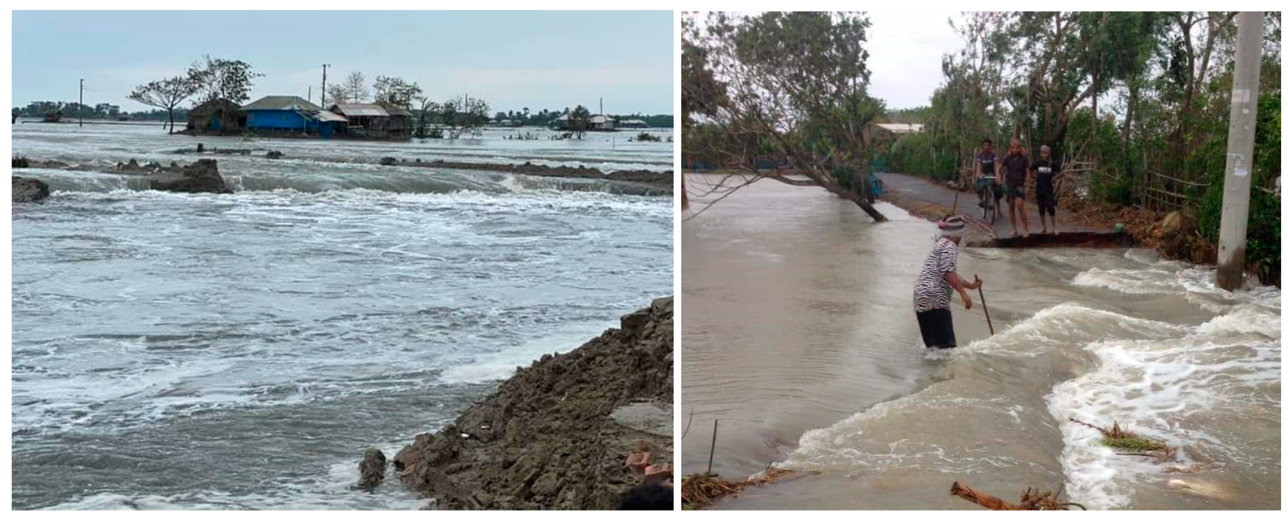
The study area is also frequently exposed to deadly tropical cyclones in the form of freshwater floods and coastal storm surges, with 17 of the 36 deadliest cyclones globally having occurred in the region [
70]. In 1970, cyclone Bhola resulted in the deaths of half a million people [
71]. Other devastating cyclones to hit the region are Sidr (2007), Rashmi (2008), Aila (2009), Komen (2015), Roanu (2016), Mora (2017), as well as Fani and Bulbul in 2019, all causing great physical and infrastructural damages, and human fatalities. Super cyclone Amphan impacted the study area with a storm surge, heavy precipitation, and strong winds from 19 May 2020 to the evening of 20 May 2020, heavily affecting 19 districts of southwestern Bangladesh. According to various estimates, Amphan caused a death toll of 26 in Bangladesh with half a million people displaced [
7,
70]. Torrential rains along with tidal surges washed away villages, livestock, fisheries, and farms with an estimated 55,667 houses and 1490 km
2 of farmland being destroyed [
7,
72]. Such damage, destruction, and the loss of lives inflicted by cyclone Amphan would have been much worse, covering an even larger area, if there were no mangrove forests along the southwest coast of Bangladesh. This natural barrier already serves as a protective wall against floods, storm surges, and tropical cyclones for the millions of inhabitants in and around the coastal rim.
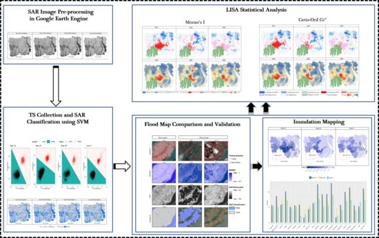
3. Materials and Methods
This study used high-resolution C-band Synthetic Aperture Radar (SAR) imagery from the European Space Agency’s satellites Sentinel-1A and Sentinel-1B. Sentinel-1 is the first satellite mission of the Copernicus Program, consisting of a constellation of two polar-orbiting satellites, acquiring C-band synthetic aperture radar images day and night irrespective of the weather [
73,
74]. Unlike passive optical sensors that require solar reflectance, an active SAR instrument transmits its microwave signal to illuminate the earth [
73,
75]. The advantage of using SAR images is that the radar pulses can penetrate thick clouds, allowing SAR to capture images in extreme conditions [
76,
77]. The attributes of SAR sensors incomputing and retrieving data in almost all weather conditions, irrespective of the intensity of sunlight, are extremely important for flood and disaster research and particularly important for a monsoon climate regime such as for Bangladesh.
Google Earth Engine (GEE), a rapidly growing cloud platform, was used to process SAR images [
78,
79]. The quality of SAR imagery depends on the mode of acquisition and raw data processing. To derive the backscatter coefficient in each pixel of SAR imagery, GEE carried out several computations before making it accessible in the cloud platform (
https://developers.google.com/earth-engine/sentinel1#metadata-and-filtering). The workflow applies a series of standard corrections including orbit files to ensure accurate position and spatial registration of SAR images. Thereafter, different categories of artifacts at the image borders are removed and the thermal adaptive noise in sub-swaths is eliminated to reduce discontinuities between sub-swaths for scenes in multi-swath acquisition mode. The images are later radiometrically calibrated using a digital elevation model to produce the unitless backscatter intensity measure. SAR images are susceptible to speckle noise derived from random signals and backscattered values. The presence of speckle noise seriously affects the quality of SAR images and the outcomes of analysis as well. Hence, several speckle filters including Lee filter [
80], Frost filter [
81] and their enhanced filters [
82], and Kuan filters [
83] were used in existing studies. A comprehensive review on SAR image despeckling can be found in [
84,
85]. Given the flat topography and the SAR polarization used for this study, we employed the commonly used Lee filter with a window size 7×7 in GEE to suppress random speckle noise of the SAR images. After processing these steps, the Digital Number (DN) values of each SAR image are converted into backscatter coefficients in the Decibel (dB) scale as σ
0 at a spatial resolution of 10 m. Finally, the backscattering profile is transformed into a linear shape. The conventional generic workflow to process/compute Sentinel-1 GRD data is described in Filipponi (2019) [
42] and DeVries et al. (2020) [
21]. We processed four temporal SAR images with both VV (Vertical Transmit and Vertical Receive) and VH (Vertical Transmit and Horizontal Receive) from the descending mode of Sentinel-1 in GGE. Cyclone Amphan affected the study area primarily on 19–20 May; thus, we obtained and analyzed a pre-event SAR image from 16 May, and three post-event images from 22 May, 28 May, and 7 June. In addition, slope, elevation, and aspect layers were extracted from a Digital Elevation Model (DEM) from the Shuttle Radar Topography Mission (SRTM). The detailed dataset and GEE assets implemented in this study are illustrated in
Table 1.
3.1. SAR Image Classification Techniques
Flooding extent mapping by utilizing SAR data provides valuable information for crisis response [
8,
14], ecology [
86], and hydraulic modeling [
36]. In the existing literature, a variety of methodologies have been used to determine the pre-crisis and post-crisis flood extent mapping [
37,
87]. These techniques range from unsupervised algorithms, such as ISODATA [
88] and K-means, to parametric supervised algorithms, such as the methodology of ascertaining the highest probability of floods. The radar backscatter threshold techniques are also commonly used, in which a SAR backscatter pixel value is labeled as a flood or non-flood by expert analysis [
31,
37,
89]. This process separates water and land pixels for images having a bimodal histogram and is often used in SAR-based flood mapping [
43]. Threshold techniques are rudimentary and robust but have limited applicability in complexcase studies, such as complex terrains, and lands with a lot of vegetation [
35,
90]. These simple methods lack the features for automatic processing, which may result in inconsistencies in the flood extent mapping for the large volumes of temporal data. Other complex classification methods of SAR images, using ancillary data coupled with machine learning algorithms, have proven to be accurate in providing almost real-time flood mapping indirect situations [
91,
92,
93]. The most commonly used machine learning-based classification techniques found in the literature review are artificial Neural Networks (ANN) [
30,
94], k-Nearest Neighbors (kNN) [
95], Decision Trees (DT), Support Vector Machines (SVM) [
96,
97], and Random Forest (RF) [
41,
52].
In earlier analyses, authors such as Rana and Suryanarayana (2019) [
87] examined floods in Assam and Kerala states in India using SAR data with RF and SVM classification techniques. Their analysis concluded that SVM performed better with SAR images to determine water and land boundaries for flood inundation extension mapping. Similarly, Dumitru, Cui, and Datcu (2015) [
38] implemented the SVM classifier with TerraSAR-X images for the quick mapping and assessment of the damages during the floods in Germany in 2013, and the tsunami in Japan in 2011. Additionally, Nandi, Srivastava, and Shah (2017) [
18] deduced satisfactory outputs with SVMs classification for floodplain mapping in Varanasi, India. Other research comprises flood susceptibility mapping executing SVM techniques to assess the likelihood of floods [
15,
97].
Given the properties to distinguish between two vectors (see
Appendix A), this study used a SVM supervised classification algorithm to differentiate the “water” and “land” backscatter values of SAR data. SVM is a non-parametric statistical learning algorithm which was originally aimed at binary classification by defining an optimal hyper plane and providing maximum parameters by segregating two classes [
98,
99,
100]. In the classification algorithm, only a subset of the data points nearest to the class boundary is used in the computation of the optimal hyperplane, and these data points are known as support vectors. In the case of nonlinear classifications, SVM can execute the classifications by using various categories of kernels which convert nonlinear boundaries to linear ones in high-dimensional regions to determine optimal hyperplanes. More detailed information and mathematical functions of SVM are provided in Vapnik (1995) [
98] and Cortes and Vapnik (1995) [
99].
In previous studies, either single-polarization, such as VV or VH, or both polarizations were used in floodwater monitoring [
32,
37]. Since SVM is a regression-based classification model, we used the VV and VH polarizations including the Digital Elevation Model (DEM), slope, and aspect as predictors to build the SVM classification model. The choice of kernel function in SVM is paramount for classification performance, and we prefer the linear kernel function due to its mathematical simplicity and computation efficiency [
93,
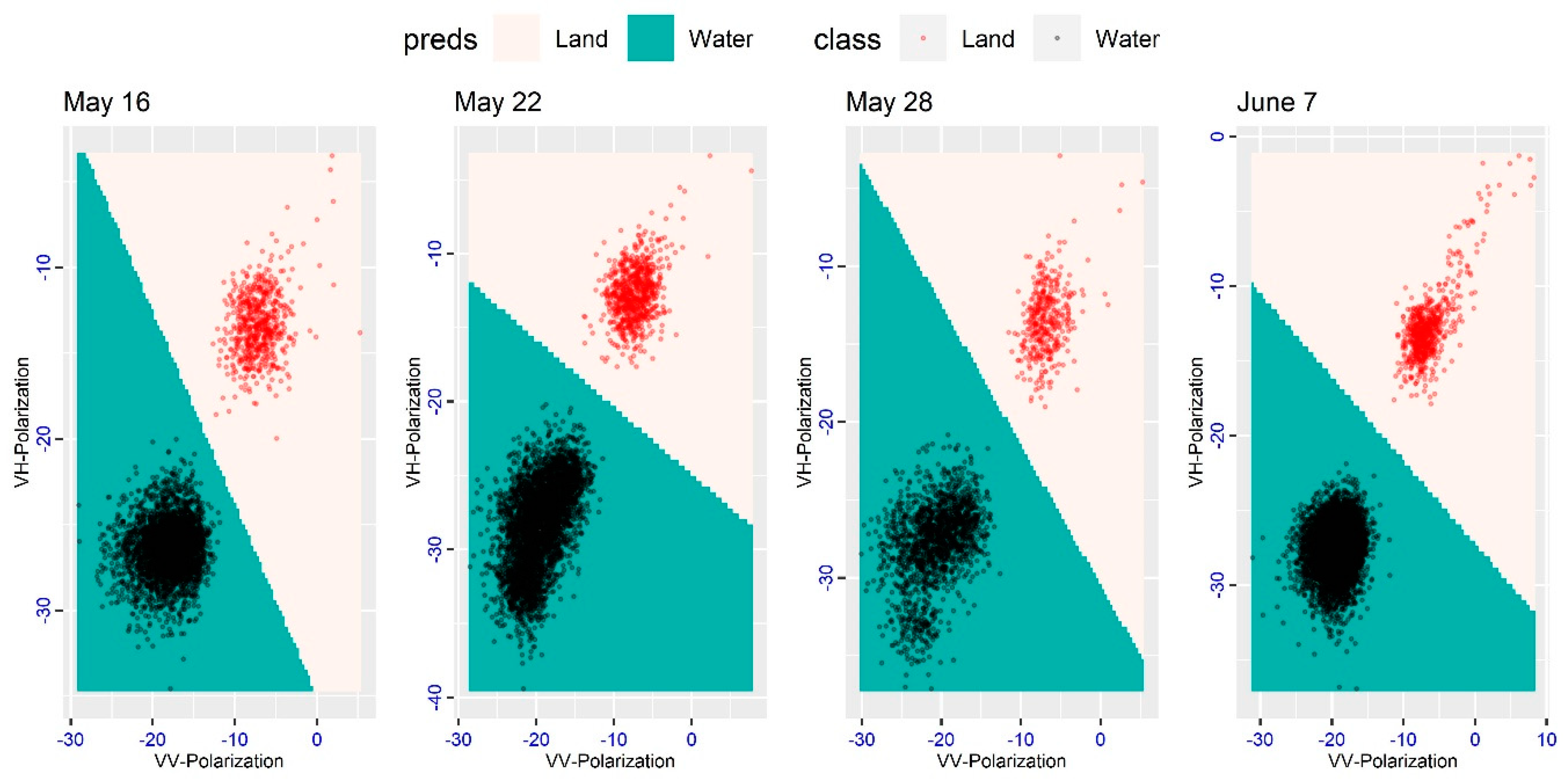
97]. The training samples were collected from composite SAR images. Water surfaces are regarded as slow intensity areas in SAR images due to low specular reflectance, whereas the surrounding terrain corresponds to a brighter intensity due to higher specular reflectance. Therefore, land and water properties of SAR images can be easily visible and divisible, and permanent water-bodies such as rivers, lakes, and ponds look darker in SAR images. These darker intensity areas in SAR images were chosen to collect training samples for various water-bodies. On the other hand, urban, infrastructure, and apparently non-flooded land sites look as brighter, and were used for the land categories training sample. In this way, we collected nearly 500 to 700 pixel values from each SAR image and used them to classify four temporal data sets with two classes—land and water—to produce one map before cyclone Amphan (16 May) and three maps after cyclone Amphan (22 May, 28 May, and 8 June).
Subsequently, the map generated before Amphan was used to exclude the perennial water from the post-Amphan thematic map; thus, we determined the extent of flood inundation water for the post-crisis periods. Finally, the inundation water was aggregated to districts, sub-districts, and the Union level for further analysis. We classified images using GEE and the raster package and we produced graphs using ggplot2 in R Studio.
3.2. Computation of LISA Statistics
LISA statistics identify local statistical patterns in spatial data. In contrast with global measures of spatial autocorrelation that outline the degree of spatial association in a single value, LISA assesses the extent to which the occurrences of similar and dissimilar values are agglomerated for each location [
59]. This method is applicable for this study because the magnitude and extent of flood inundation can be measured within a defined spatial scale. Though there are many methods to compute patterns in spatial data, the most common and popular LISA statistics are Local Moran’s I and the Getis–Ord Gi* statistic [
61]. To compute the LISA statistics, we combined flooding areas at a lower administrative level, locally called “Union” and the percentage of each Union affected by flooding were calculated. Later, two LISA statistics; the Local Moran’s I index [
59] and Getis–Ord Gi* index [
101], were computed at the Union level to map spatial clustering and flooding hotspot across the affected region of cyclone Amphan. The LISA statistics enable us to detect pockets of spatial association that may not be visible when using global statistics.
3.3. Getis–Ord Gi*
Getis–Ord Gi* statistics examine the places or regions where there is a statistically significant spatial clumping of higher magnitudes of a variable, independent of the number of observations [
101]. The Getis–Ord Gi* statistic displays z-scores (standard deviations) and
p-values (statistical probabilities) that indicate if the attribute results are statistically clustered, and the larger z-scores and lower
p-values indicate a spatial clustering of high occurrences of hotspots or a high probability of flooding in the given period. Conversely, a spatial unit with low z-score and high
p-value indicate a spatial clustering of a lower occurrence of hotspots or a low probability of flooding in the given period. A z-score near zero indicates no apparent spatial clumping for the geographical unit being studied. The z-score for every region
i is computed as:
where
represents a probability of flooding within given spatial units (i.e., Union),
is a spatial weight which defines the neighboring Union
,
is the sum of weights
,
is the mean of the Union level inundation rate, and
is the standard deviation of the
values.
3.4. Univariate Moran’s I
The Local Moran’s I compute the degree to which geographic objects or events are clustered, dispersed, or randomly distributed [
59,
60,
102]. Moran’s-I is a useful tool for deriving hotspots, and for classifying them into spatial clusters and outliers. The Local Moran’s-I differs from the Getis–Ord Gi* statistic where the covariance rather than the sums are computed. The standard univariate Moran’s I statistics for remote sensing applications take the following form:
Where
n is the number of spatial units (in this study,
n = 1165),
is the spatial weight between unit
and
,
is the value of unit
,
is the mean value and
is the standard deviation. The weight
can be determined using a distance band or a spatial contiguity matrix. This statistic calculates a z-score, a
p-value, and a code representing each class of clump into four statistically relevant results. A highly positive Local Moran’s I value implies that the locations under investigation have high or low values similar to its neighbors; thus, the locations are considered spatial clusters [
59,
103]. Spatial clusters can be categorized as “high-high” (high values in a high-value/risk neighborhood) and “low-low” (low values in a low-value/risk neighborhood) [
103]. A high negative Local Moran’s I value means that the location under observation is a spatial outlier. Spatial outliers have values that vary from the values of their surrounding locations. Again, these include “high-low outliers” which mean high value in low value neighborhoods and “low-high outliers” that exhibit low value in high value neighbourhoods. To compute LISA statistics, the estimated flooding areas of 22 May, 28 May and 7 June were calculated for the 1162 Unions (lowest level of administrative units, locally called “Unions”) in the area under survey. In determining the spatial weight for the Getis–Ord Gi* and Moran’s-I, the second-order queen’s contiguity index of the neighborhood was assigned for individual Unions. Contiguity weight measure was preferred as this weight measure performs better with a problem of the uneven distribution of neighbor cardinality. The contiguity weight matrices and both LISA statistics were computed in the GeoDa software. The hotspot and cluster of flooding waters were deduced to be statistically significant at 99.99% (
p < 0.001), 99% (
p < 0.01), and 95% (
p < 0.95) confidence levels. We assume that the application of LISA statistics will provide useful and critical data on change and variation of floodwater coverage and intensity over larger geographical areas and such information can be used as important indicators for flood disaster management.
4. Results
4.1. Accuracy of Flood Mapping
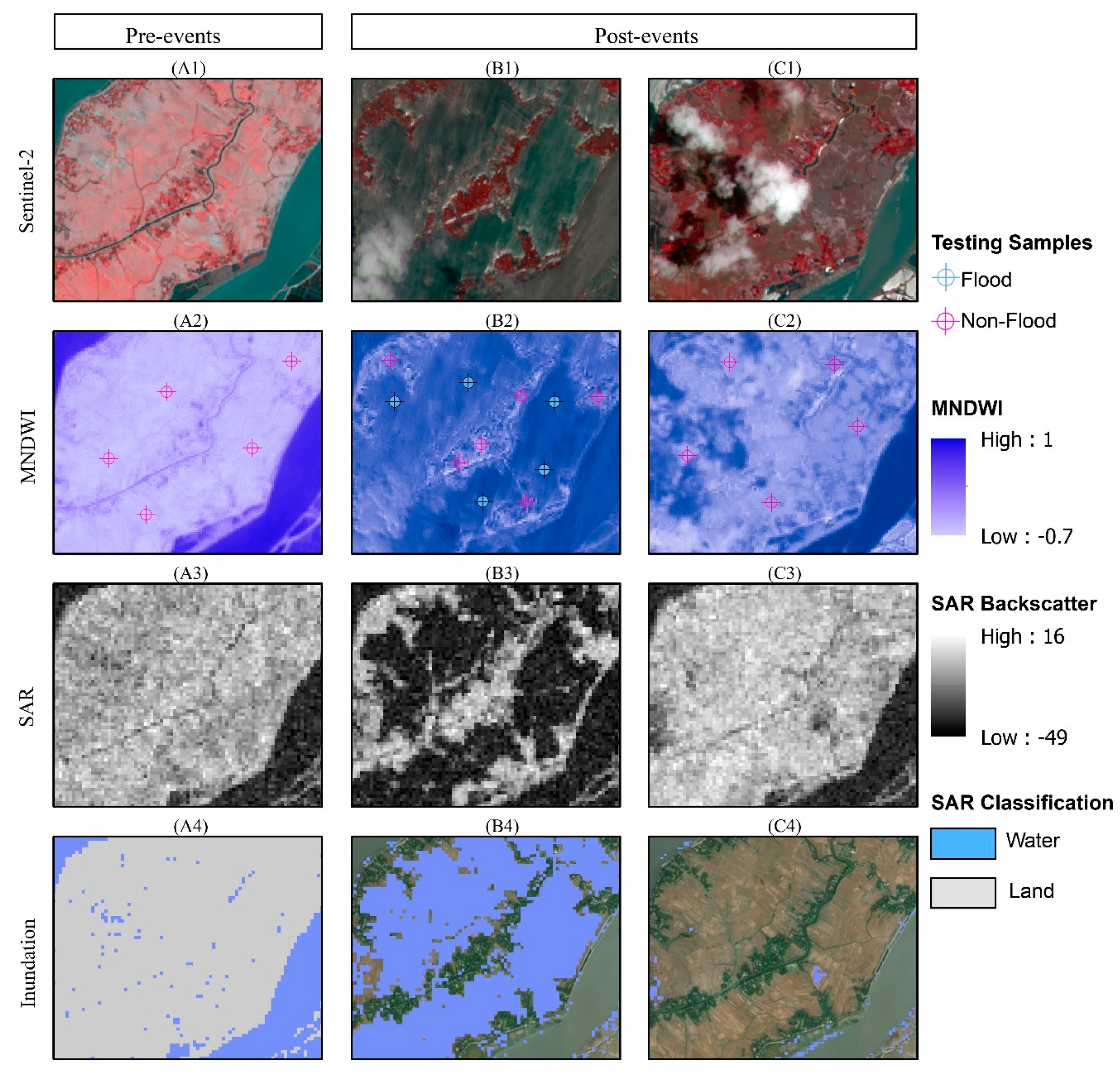
To ensure the authenticity and accuracy of the analysis, a flood map evaluation was performed based on visual comparison and testing samples that were retrieved from the Modified Normalized Difference Water Index (MNDWI). The MNDWI maximizes the high reflectance of water by using the green wavelength and minimizing the low reflectance of the Mid-Infrared (MIR) wavelengths of water features. Thereby, water attributes with their positive values are amplified in the data, whereas vegetation, soil, and other non-water attributes with close to zero or negative values are suppressed. Owing to its ability to delineate water and non-watery features using MIR and Green bands of multispectral imagery, MNDWI has been widely used in many remote sensing applications, especially in assessing flood maps derived from SAR imagery [
12,
104,
105,
106]. Using Green and MIR wavelengths of available multispectral imagery from Landsat-8, and Sentinel-2, MNDWI was computed (Green-MIR/Green+MIR) in GEE. The accessible multispectral imagery that is close to the SAR-acquired date in the study regions are 16 May, 25 May and 8 June. Since large sections of these images are under a thick cloud cover (ranging from 30% to 70%) during the researched periods, a relatively cloud-free area was chosen to extract the testing samples. Thus, we collected 170 testing samples from the computed MNDWI on 16 May, 53 samples from 25 May, and 103 samples from 8 June to evaluate the flood maps of 16 May, 22 May, and 7 June respectively. The accuracy of the flood maps were assessed using the omission and commission errors within the confusion matrix and kappa statistics. The kappa statistics compute the similarity between signature samples and control samples. The overall classification accuracy obtained from all the images ranged between 95% to 97% with a kappa coefficient that ranged between 0.92 to 0.98. The highest overall accuracy of 97% was quantified from the images of 16 May and 22 May (98%), while the least overall accuracy was 95% for the image accessed on 7 June. Similarly, the derived average user and producer accuracy of both classes was almost 95%. The highest user accuracy was derived for water classes which correspond to 98% precision for 16 May, 22 May, and 7 June respectively. The overall high classification accuracy for the flood inundation mapping before and after cyclone Amphan indicates that the flood maps are reliable for further statistical analysis. Due to the lack of available multispectral imagery, the validation for the flood map on 28 May was not possible. However, a close examination using the nearest acquired-date multispectral imagery such as 25 May and 3 June shows that both of the categories (land and water) were well distinguished. We provided a comparison of flood extents with multispectral imagery in
Appendix B.
4.2. Extent of Post-Amphan Flooding
Information on flood inundation extent and change over time is important for understanding changes in societal exposure, volumes of water storage, flood water attenuation, and for management of flood hazards. Super cyclone Amphan struck the coast of Bangladesh accompanied by strong winds and torrential rain on 19–20 May 2020, and these conditions persisted for several days.
The rainfall data derived from CHIRPS in the study area shows that an average of 200 mm of rainfall fell in association with Amphan. Among the 16 affected districts surveyed, the highest rainfall measurement was recorded at Jessore (220 mm), Satkhira (136 mm), and Narail districts (132 mm), while the lowest rainfall was recorded at Bhola (23 mm) and Lakshmipur (22 mm) districts. Such widespread rainfall within a short duration coupled with the storm surge resulted in flooding across vast areas in the coastal regions of Bangladesh.
The flood water derived from the post-Amphan SAR image shows that 2233 km
2 of land was inundated on 22 May, revealing the repercussions and severity of cyclone Amphan (
Figure 3). Among the affected districts, Bagerhat, Pirojpur, Satkhira, Barisal, Jessore, Patuakhali, and Khulna received the highest water inundation during the cyclone. The flood areas obtained from SAR images of 22 May show that these seven districts were inundated by 335, 248, 213, 211, 190, 188, and 173 km
2, respectively. In terms of percentage of land inundated by floodwater for each district, Jhalokati, with the smallest area of the districts surveyed, had nearly 19% of its area inundated by floods on 22 May, while Pirojpur and Bagerhat were flooded 17% and 12% by area, respectively. Barisal and Satkhira were inundated over 7% by area. Jessore and Barguna were each inundated 6% by area.
Later, the floodwaters had abated to 1490 km2 on 28 May, before the affected areas jumped to 1520 km2 on 7 June, linked to floodwaters upstream making it to the lower coastal regions. Similarly, following the immediate consequences of cyclone Amphan, floodwaters started receding from nearly all the flooding districts except Satkhira where extended flooding was observed through 7 June. In the district of Pirojpur, the flood subsided to 85 km2 on 28 May from 249 km2 on 22 May and it further reduced to 29 km2 on 7 June. The districts of Barisal, Jhalokati, Patuakhali, Jessore, and Bagerhat had a similar trend where the flood abated by 109, 104, 53, 103, and 11 km2 respectively between 22 May and 7 June. The districts of Lakshmipur and Barguna had consistent floodwater by the end of the duration of the study. The fairly rapid reduction in flood water extent does highlight the need for rapid analysis following such events, to accurately map impacted areas and prevent under estimation of impacts.
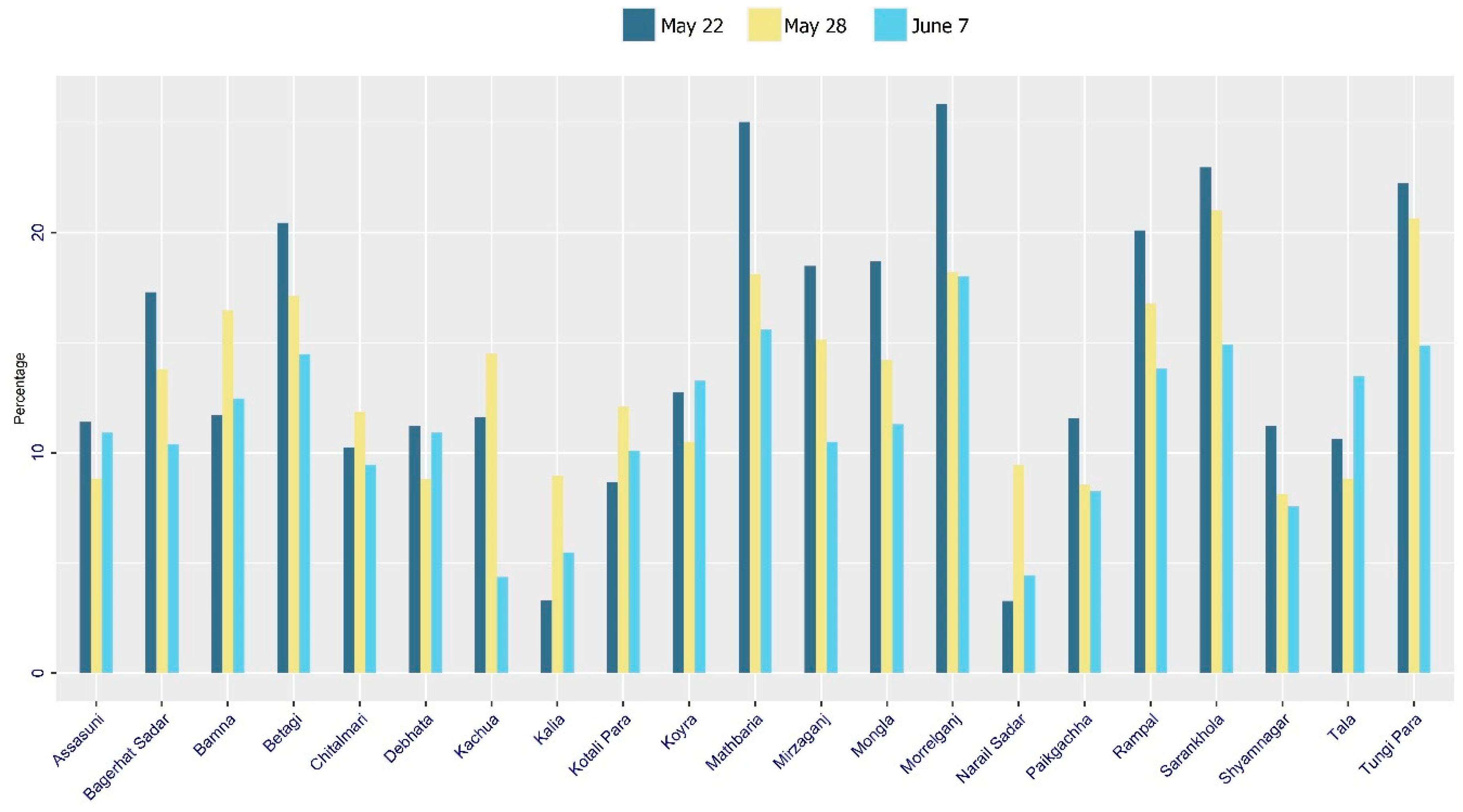
At the sub-districts level (
Figure 4 and
Figure 5), several sub-districts such as Rajapur and Kathalia in Jhalokati district, were submerged by 32% and 27%, respectively on 22 May. Morrelganj and Sarankhola in Bagerhat district were inundated by 26% and 23% respectively. In Pirojpur district, Zianagar and Mathbaria were flooded at 23% and 22% respectively. Other major flooded sub-districts were Bakerganj in Barisal district, Betagi in Barguna district, Koyra in Khulna, and Shamnagar in Satkhira. These sub-districts were inundated to the extent of 79, 34, and 52 km
2 respectively. The changes of inundation areas (as percentages) in each sub-district are illustrated in
Figure 4 and
Figure 5.
4.3. Spatial and Temporal Variability of Getis–Ord Gi*
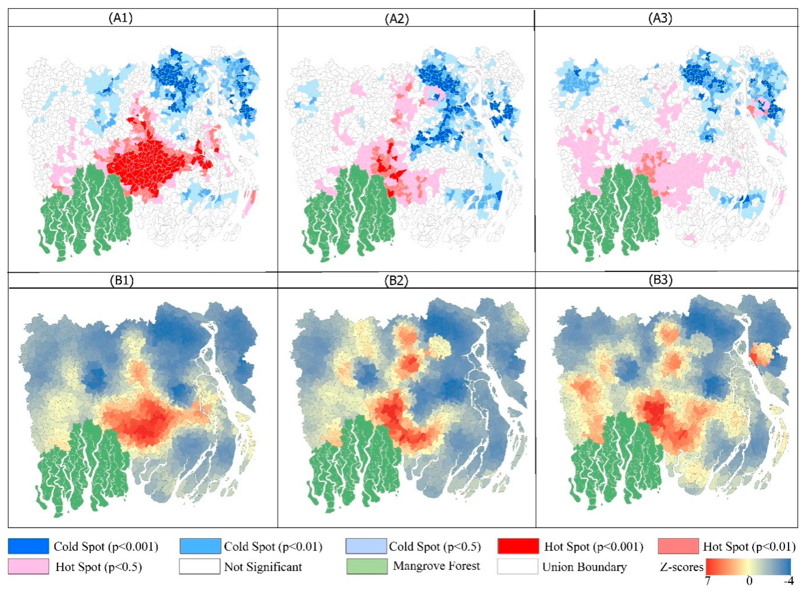
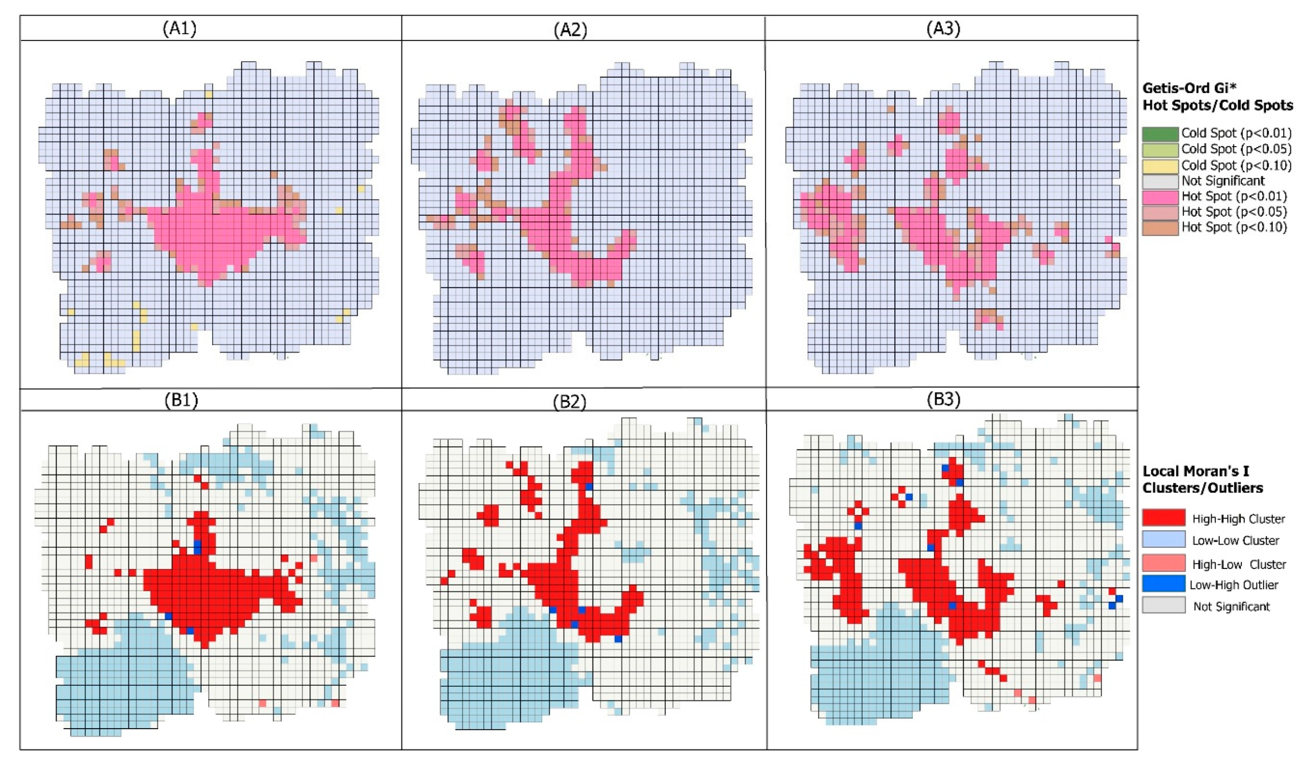
Getis–Ord Gi* depicts the statistically significant spatial clustering of incidences where the high and low values are located, and thus it identifies the occurrences of hotspots and non-hotspots. In this study, we employed this technique to deduce the precise location of statistically significant clusters of inundated areas, i.e., flooding hotspots. The results of Getis–Ord Gi* (
Figure 6) indicate that the statistically significant flooding hotspots are mainly clustered in the central part of the study area, adjacent to the north eastern region of the mangrove forest. The statistically significant negative z-scores of Getis–Ord Gi* are less concentrated geographically, and they are mainly found in the far north eastern regions of the study area.
On 22 May, a total of 238 Unions were identified as hotspots of flooding (
p ≤ 0.05), 101 of them being highly significant hotspots with
p < 0.001, 60 of them were hotspots with
p < 0.01, and 77 flooding hotspots with
p < 0.05 (
Table 2). Bagerhat district exhibited the maximum number of flooding hotspots triggered by cyclone Amphan (
p ≤ 0.05) where a total of 52 flood hotspots were identified on 22 May followed by Pirojpur (46), Jhalokati (26), Barisal (16), Bhola (16), and Khulna (15) (
Table 3).
Among these high statistically significant flooding hotspots, 35 hotspots with p < 0.001 were identified in Pirojpur districts, while 23 are located in Bagerhat, followed by Jhalokati, Barisal, and Barguna. Each district had a flooding hotspot with p < 0.001 at 15, 9, and 8 respectively on 22 May. Later, the number of flooding hotspots identified in the study area dropped to 166 (p ≤ 0.05) in the 2nd week (28 May) after cyclone Amphan. During this period, 8 high flooding hotspots with p < 0.001 were identified in the central region, where 33 hotspots had p < 0.01 and 125 were identified flooding hotspots with p < 0.05. Again, Bagerhat district had the highest number of flooding hot spots; a total of 50 hotspots with p < 0.05, and 7 of them had p < 0.001. Though it was observed that the flood affected areas had decreased in the second week of Amphan, some new areas were reported as having increased flooding at the beginning of June due to additional rainfall and riverbank failure across the southwest part of this study and the inland waters making their way towards the coast within the rivers with their flood waters. As a result, both affected areas and the number of flooding hotspots witnessed a surge on 7 June, when the total flooding hotspots were identified as 208 (p ≤ 0.05). This time, increasing hotspots were found in the Satkhira district; 27 Unions were identified hotspots (p ≤ 0.05); then 3 Unions on 28 May and 11 Unions on 22 May.
In areas where Getis–Ord Gi* values were substantially contrasting to the surroundings; they were considered as neither hot spots nor cold spots. They are indicated as not significant because they did not have as great of a geographic extent of flood water compared to the more widely affected areas. Such areas of “Not statistically significant” increased through the study period. As such, on 22 May a total of 457 Unions detected a non-statistically significant inundation rate, while on 28 May, this number rose to 658 and then to 614 on 7 June. This illustrates that some areas were inundated after Amphan due to heavy downpours but eventually rainwater flowed back into the river. As a result, flood-free zones increased considerably once the immediate flooding in the aftermath of cyclone Amphan began to subside.
4.4. Spatial and Temporal Variability of Local Moran’s I
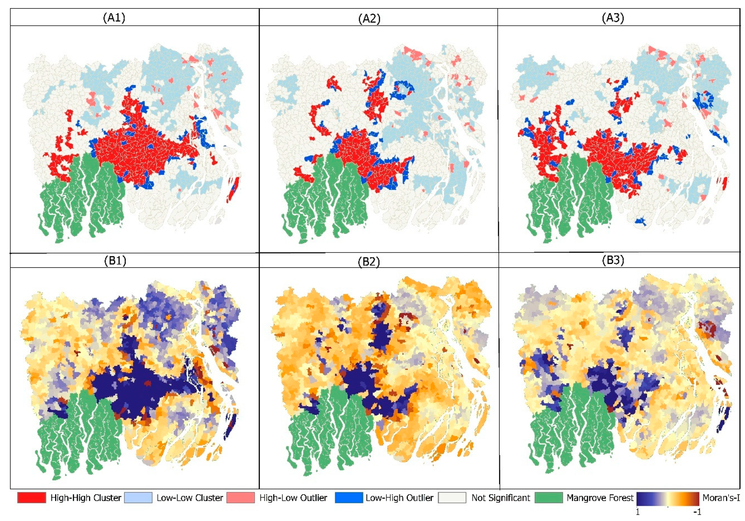
The Local Moran’s I statistic quantifies the degree of spatial autocorrelation at each specific location [
59]. The result of Local Moran’s I and z-scores (
Figure 7) illustrate the locations over which Amphan-triggered inundation occurred and how the spatial distribution of the flood extent changed over the fortnight after cyclone Amphan. In
Figure 7, regions in red High-High clusters (HH) indicate higher than average inundation values located by neighbors that also have higher than average flooding. Similar to the Getis–Ord Gi* analysis, the Moran’s-I statistics depicts those Unions that are located in the central areas and demonstrate the exceedingly high statistically significant cluster of flooding. The most significant cluster of positive spatial autocorrelation decreased in size from 22 May to 7 June (
Figure 7(B1–B3)); the global mean values of local Moran’s-I statistic decreased from 0.46 to 0.17. This result indicates a general decrease in spatial clustering of flooding in the second week after cyclone Amphan. In the immediate aftereffects of Amphan, 188 Unions had high Moran’s-I values with a statistically significant
p-value of less than 0.001. In the weeks following the cyclone, the number of Unions associated with highly significant
p-values (
p < 0.001) declined to 112 on 28 May but showed a bounce back up to 144 at the end of the study period. Similar to the Getis–Ord Gi* analysis, these highly significant spatial associations using Moran’s-I are mainly observed in the Bagerhat district as well as the Pirojpur, Jhalokati, Barisal, and Khulna districts.
Areas in light blue (in
Figure 7) indicate a Low-Low cluster (LL), having lower than average inundation located by neighbors with lower than average inundation rates. During the post-Amphan periods a total of 345 Unions were detected as being in LL inundation clusters (
p < 0.001) on 22 May, whereas 313 and 311 Unions were in LL clusters on 28 May and 7 June respectively. These LL clusters were mainly located in the Chandpur, Barisal, Madaripur, Khulna, and Shariatpur districts. Areas in the blue Low-High outlier category (LH) revealed locations where inundation rates are below average, but neighbors have above average inundation. They have a low negative z-score for the location and were classified as a Low-High outlier. These LH outliers of flood occurrence were found in 50 Unions on 22 May, 54 Unions on 28 May, and 64 Unions on 7 June with a statistically significant
p-value (
p < 0.001). Areas in pink demonstrate High-Low outliers (HL) where inundation rates are above average, but neighbors have below average values. In total, HL flood occurrences were identified in 25 Unions on 22 May, 34 Unions on 28 May, and 27 Unions on 7 June. These HL and LH clusters are sporadically distributed across the study area but mainly detected in the districts of the Barisal, Khulna, Bhola, and Chandpur.
5. Discussion
Super cyclone Amphan caused massive flooding and destruction along its path across the coastal belt of Bangladesh. This study utilized publicly available SAR data from Sentinel-1 to quantitatively examine the spatial variation of flooding triggered by cyclone Amphan within 16 coastal districts of southwestern Bangladesh. Our study demonstrates that the image collected on 22 May shows the greatest flooding extent, demonstrating the widespread consequences of cyclone Amphan. On 22 May, approximately 2233 km
2 was inundated, which accounted for 8% of the study area. An initial decrease in the flood extent was observed by 28 May when the total inundation area dropped to 1490 km
2. The results also revealed that there was a further spike in flooding in the third week after Amphan, when some areas reported consistent flooding. As a result, flood-affected areas under the survey were estimated to be as much as 1520 km
2 on 7 June. One probable hypothesis for some regions becoming newly flooded on 7 June is due to additional downpours in the first week of June and rainwater, which landed upstream making it downstream as a storm surge, causing additional stream flooding. The rainfall data presented in (
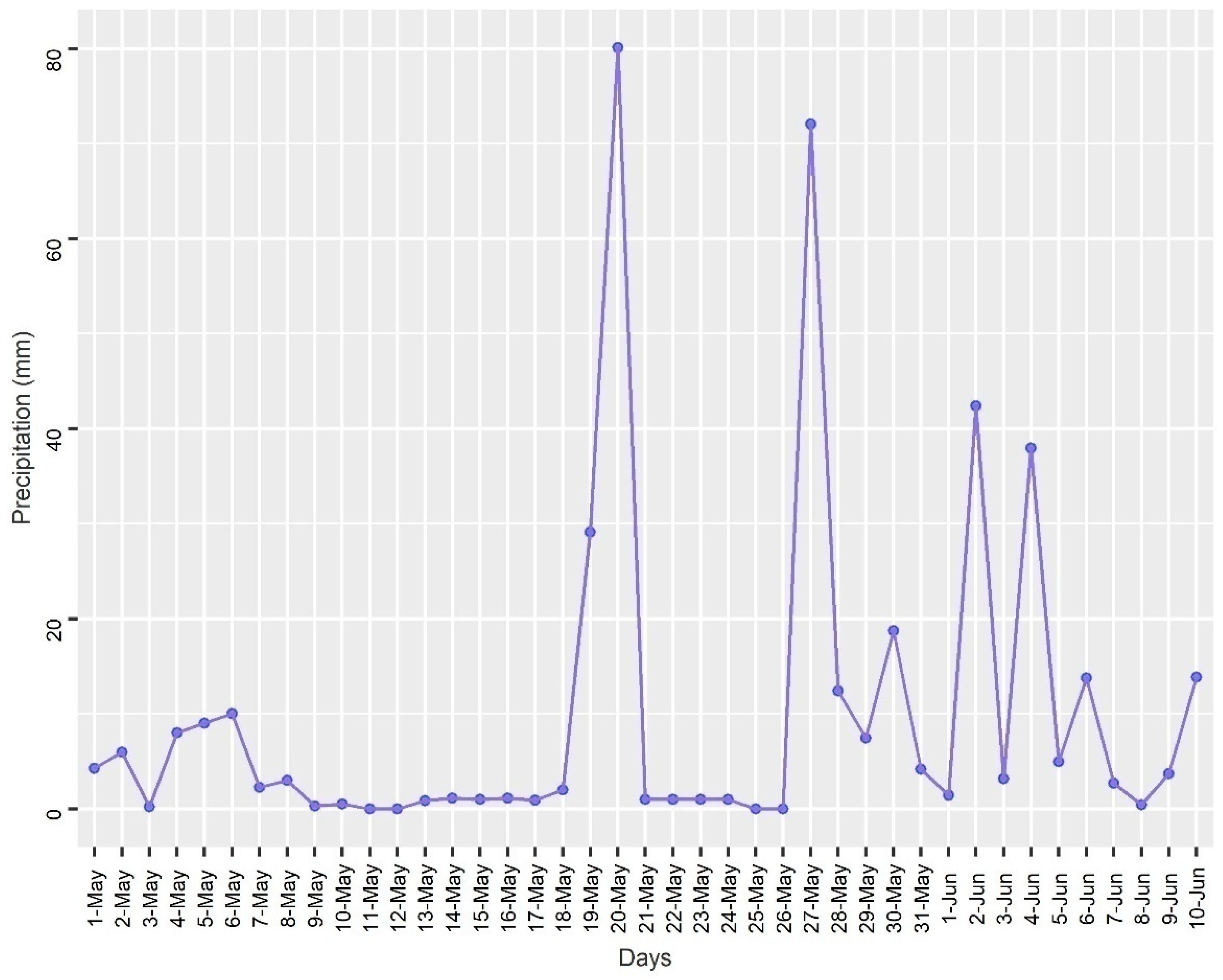
Figure 8) show that the average rainfall received in the study area was approximately 40 mm between 2 June and 5 June. Moreover, riverbank failure along with coastal polders and dikes were reported to have broken out due to increased volumes of surface runoff in south western regions of the area that was eventually resulting in incessant flooding [
7]. This extended duration of flooding was observed in Satkhira districts where 13 Unions were reported to have been newly flooded on 7 June.
The ubiquity of flooding may correspond with favorable geophysical, topographical, and land cover elements. Within the academic framework, such a geophysical variable has been prioritized in earlier research across the area under study [
107,
108,
109,
110]. Many of the existing studies [
8,
9,
10,
12,
13,
16,
19,
20,
26], however, are dedicated to simply flood mapping which undermine the need of rapid flood assessment and subsequent relief implementation. It is paramount to determine how such floodwaters are distributed and how their locations are fluctuating in time and space, and how they are related to specific geographical territories. Having knowledge of spatial and temporal distribution patterns of flooding and the trend of their agglomerating or dispersing that are statistically distinct from random spatial patterns, disaster managers can ascertain better measures in responding to the evolving crisis. As such, disaster managers need actionable data highlighting the regions that need prioritization compared to other regions across the large affected area. Hence, we assert that a simple flood mapping or ratio computation of flooding water at a local spatial scale would not suffice for studying this heterogeneity, as this measure would not indicate how different regions compare with each other in terms of statistical significance. As such, the methodologies presented in this research are superior in performance, as LISA statistical techniques enable us to categorize and provide a quantitative assessment of spatial data that emphasizes the probability and extent of potential disasters that are clustered, dispersed, or simply randomly distributed in a geographical area. LISA has been utilized to reveal emerging trends in spatial data and this application has been reported in a wide range of ecological studies. The application of LISA in the mapping of the geographical discrepancy of flooding occurrence, however, has not been seen in any previous application. Hence, this study contributes new knowledge in several ways. Firstly, we combine active remote sensing data with LISA statistics to quantify the extent and regional variation of flooding at different spatial scales. We employed commonly used LISA statistics such as Moran’s-I, which calculates the degree to which geographic events are clustered, dispersed, or random at a local spatial scale. Hence, the simplicity of our employed method, readily available data sources, and rapid assessment post-disaster which is critical for management and disaster relief implementation are actually a huge strength of this research—making this approach readily useable across the world. The other frequently used LISA index is Getis–Ord Gi*, which measures the degree of clustering for either high or low values. The main strength of the Getis–Ord Gi* analysis is that it identifies clusters that are not merely regions of high-flooding density but regions of statistically significant high-flooding density, which provides analysts with an empirical measure of spatial heterogeneity. Alternatively, the advantage of using Moran’s-I is that it computes the spatial dependence in a given set of geographic data. In other words, it measures the spatial autocorrelation of a variable according to its geographical location [
100]. In our study, both LISA statistics of Getis–Ord Gi* and Local Moran’s I were able to explicitly delineate regions associated with homogenous and heterogeneous patterns of flooding. The more homogenous flooding areas revealed a high positive spatial autocorrelation as observed by both Local Moran’s-I and Getis–Ord Gi* statistics. Small, isolated, and scattered flooding belts were characterized by a low positive and negative spatial autocorrelation.
Such spatial variances of disaster occurrence highlight their concentration on the map and can be an important objective tool for the experimental investigation of causes of flooding occurrence upon which an effective flood response and mitigation strategy can be implemented to control future flooding occurrence and damages. Therefore, this methodology is an important contribution to quickly identify flooding hotspots given the need for timely response especially in the developing countries with limited resources, such that these methods will allow for quicker and more effective targeted response efforts where most critically needed.
In previous studies, single-polarization images with either VV or VH of the SAR band were used to examine the extent of flooding. Some studies used both VV and VH polarizations and compared their suitability to flood mapping. Such examples include Clement et al. (2018) [
37] who compared the inundation results between VV and VH, and found that VV polarization had fewer misclassifications than VH. Similarly, Twele et al. (2016) [
111] and Uddin et al. (2019) [
20] deduced that VV polarization provided slightly better accuracy to VH. Meanwhile, other studies including Carreño Conde, and De Mata Muñoz (2019) [
8] and Ezzine, Saidi, Hermassi, Kammessi, Darragi, and Rajhi (2020) [
36] concluded that using VH polarization in their studies accomplished the best results for flood mapping. However, it is still unclear which of the two Sentinel-1 polarizations is the primary choice for delineate flooding. In this study, we employed ensemble techniques with both VH and VV polarizations combined with DEM, slope, and aspect to delineate flooding areas from SAR images. In such methods, the contribution of each band and the associated predictors to the model performance and classification are estimated and reported individually in scales between 0 and 100. By implementing this approach, we could avoid the uncertainty and ambiguity of selecting the best polarization band, permitting a cumulative contribution of each indicator to the best classification performance and output.
Though the outcomes of LISA statistics to ascertain potential flooding hotspots or agglomerations are promising, the study has several methodological limitations. The first limitation is the combination of flooding data into Unions (smallest administrative units) which have different spatial extents. The study area consists of 1162 Unions, covering an area of 26,738 km
2 (excluding mangrove forest). The dimensions of the 1162 polygons range from a minimum of 0.22 to 127 km
2, with a mean value of 23 km
2. Data aggregation within such ranges of sizes of geographical units may have affected our analysis of LISA statistics. In such circumstances, the Modifiable Areal Unit Problem (MAUP) occurs with a high probability of affecting the result. Referring to the data aggregation problem stated above, we further examined whether data aggregation to Unions influenced the performance and output of LISA. Since the calculation of an appropriate grid cell size is highly controversial and there is not currently a consensus in academia, we determined each grid cell size by considering the average areal size of Unions, which is 23 km
2. Hence, we created a rectangular grid of the size of 4796/4796 m which corresponds to the area of each gird cell that is approximately 23 km
2. In this way, we created a total of 1665 grid cells covering the entire studied area. Later, the proportions of the inundation rate were computed and aggregated to individual grid cells before they were used for LISA analysis. The scaling of data aggregation at Union versus gridding and its influence on clustering and hotspots analyses are presented in
Appendix C. The comparison of the results based on a grid cell with the results based on aggregation by Unions shows that the LISA output was affected by zonation effects. Data aggregation by the grid cell increased the number of inundation clusters and hotspots while reducing the number of unaffected locations. This is because the number of analysis units for the grid is higher than the Unions. However, a thorough examination of the output of both Union and grid-based LISA outcomes shows that the inundation hotspots and agglomerations within the grid and Union are very similar. In both spatial scale analyses, inundation hotspots and clusters are mainly spotted in the central regions of the surveyed area; though several hotspots for the 7 June map at the grid-scale are eliminated in the north eastern belt of the studied area. Since the objective of this research is to ascertain the hotspots of flooding; such minor effects on the performance of LISA from zonation would not largely affect the importance of these detections. Hence, our analysis was conducted solely upon Unions.
Additionally, each of the techniques adopted in this study has its advantages and deficiencies. The Getis–Ord Gi* identifies clusters of high or low values, but it does not detect a negative spatial autocorrelation (spatial outliers). Local Moran’s I, on the other hand, can detect both positive and negative spatial correlations. The Getis–Ord Gi* statistic has been preferred in some case studies as it matches the usual definition of a cluster and is indicated for use with variables that constitute the natural origin [
112]. Geary’s C is another computation method of spatial autocorrelation, which emphasizes the variances in small neighborhoods and is statistically less well-behaved than local Moran’s I. Therefore, Moran’s-I is usually preferred to Geary’s C [
113].
Though SAR data provide excellent delineation of flood extent mapping during all weather conditions and day and night, uses of such data, however, is not exclusively straightforward. SAR images are effective for mapping smooth, and open water bodies, however, emergent vegetation, dense tree cover, rough winds, and a turbulence environment can increase radar back-scatter returns, making delineation of inundated areas problematic [
114]. Hence, a combination of visible and near infrared bands (e.g., Normalized Difference Vegetation Index) from passive remote sensing data and multi-frequency polarimetric SAR data with other ancillary data including land cover maps, DEM, river network, etc., will be used for future study.
Since a majority of the flood-prone areas were inaccessible due to COVID-19 lockdown and due to the communication network being completely cut off due to the flooding, a robust validation from ground observation data was infeasible. Hence, flood maps were validated using a surrogate computation methodology from MNDWI, derived from NIR and Green bands of Sentinel-2 data. This approach has been extensively used in earlier studies for extracting floodwaters and validation of SAR-based binary mapping [
12,
18,
104,
105,
106]. We also used the visual comparison of SAR backscatter reflectance, MNDWI, and classified flood maps to verify that floodwater extracted using SVM learning corresponds well with apparently shown water-bodies on existing SAR images and MNDWI (
Figure A2 of
Appendix B). Such methodologies were also employed in studies conducted by Gan et al. (2012) [
77]; Grimaldi et al. (2020) [
114], and Martinis et al. (2018) [
115]. For more validity and accuracy in the flood maps derived from SAR images, further evaluation is recommended using robust ground truth data combined with stream gage information.
6. Conclusions
Quantifying the spatial heterogeneity of flooding disasters is of considerable importance, both for an immediate response and understanding the areas of greatest need for assistance, but also in the longer term for developing adaptive management measures for communities and building location-specific resilience to impede the impacts of the disaster. Simple flood mapping and analyses at local scales, however, bear a challenge to differentiate a region that is highly vulnerable to flooding disaster occurrence from a location that is vulnerable in general. Here, we analyzed the post-Amphan flooding extent and spatial variation across the affected coastal districts of Bangladesh. We employed LISA statistics, a powerful computational method for extrapolating the degree of flooding occurrence at Unions, which can be used to complement the visual assessment of flooding propensity at a local scale by disaster managers. In particular, we have shown that identifying the region of flooding using the image analysis can allow the application of spatial statistical tools to effectively compute the spatial heterogeneity in the flooding incidents, which can add valuable information for rapid, proactive, and operational flood management. The results indicate that there is a high spatial variability in the occurrence of flooding that was characterized by LISA across the surveyed region. Predominantly, the area of the central locales associated with low altitudes (i.e., Bagerhat, Khulna, Barguna, and Barisal districts) demonstrated the highest inundation caused by cyclone Amphan. This area was also associated with a high z-score and Moran’s I, signifying that the identified locations are more vulnerable to any type of flooding. Additionally, the average mean z-scores and I-scores reveal a receding trend over time, indicating that the spatial variation and magnitude of flooding clusters occur initially with a high magnitude and larger clusters, which convert to the low magnitude with comparatively smaller clusters by the end of the study period. By maximizing the advantage of LISA utilities, this study enabled us to uncover the flooding anomalies of high and low concentrations in what is otherwise characterized as a homogenous inundation area when using simple flood mapping techniques. The approach presented in this study may be of great interest for disaster managers for future study such as local regions of spatially explicit high or low flooding. The shortcomings of this study included the use of MNDWI to evaluate the flood maps, which may be good for interim validation purposes. However, a robust validation incorporating ground-based training samples combined with information over stream flow discharge is recommended for improved reliability and performance of the products. Refinement in the methodology can be addressed, particularly in the flood data aggregation at the Union or artificial grid cell, which may have affected our results. Hence, a sensitivity analysis with different spatial scale data aggregations is needed to adopt and implement the best combination for examining flooding hotspots and clusters. Future work is recommended to integrate ground data, land cover information, stream gage data, and predictive models to achieve a long-lasting flood management goal throughout the coastal regions of Bangladesh.

 ,
, 


