Patch Pattern and Ecological Risk Assessment of Alpine Grassland in the Source Region of the Yellow River

Abstract

The source region of the Yellow River (SRYR) is an important water conservation and animal husbandry resource in China. It is of great significance to understand the patch pattern and ecological risk of alpine grassland in the SRYR for ecological environment management. This study first used 12 unmanned aerial vehicle (UAV) aerial images and eight moderate resolution imaging spectroradiometer (MODIS) vegetation index product MOD13Q1 images from July to August in 2019 to extract alpine grassland patch patterns in the SRYR, then constructed an ecological risk model based on the landscape vulnerability index and landscape disturbance index, and finally combined spatial self-reliance correlation and semi-variance analysis methods to explore the spatial distribution of ecological risks. The results showed that the patch fragmentation degree (Pi), area weighted shape index (AWMSI), and separation degree (Si) of the four grassland types in the SRYR are ordered as follows: alpine steppe > degraded meadow > alpine meadow > swamp meadow. Moreover, the greater the fractional vegetation cover (FVC), the greater the landscape dominance index (DO_i), and the better the ecosystem stability. The spatial difference of ecological risk in the SRYR shows a situation of low risk in the east (ERI_min = 1.5355) and high risk in the west (ERI_max = 70.6429). High FVC was found in low and mild low risk areas where the vegetation types are mainly swamp meadow and shrub, while low FVC was found in high and mild high-risk areas where the vegetation types are mainly alpine steppe and degraded meadow. The spatial distribution of ecological risk of the SRYR has obvious positive spatial correlation (Moran’s I = 0.863), the spatial aggregation distribution is distinct, and the local space has significant high-high aggregation and low–low aggregation phenomena. The results of this study reveal that patch characteristics have good indicative significance for alpine grassland ecological protection and should be considered in future studies. In addition, the ecological risk in the SRYR is relatively high, especially in the western region, which should be taken seriously in future ecological management and governance.

1. Introduction

Fragile ecosystems are defined as lacking natural resilience or by being impacted heavily by an unnatural (human) event that it changes in an unexpected or undesired way [1]. It is estimated that by 2025, fragile ecosystems will account for about 45% of the earth’s land area [2]. Ecosystem stability is a necessary prerequisite for human survival and socio-economic development. Systematic analysis, maintenance, and stability of the ecosystem are important areas of research in the current field of ecosystem research. In recent years, under the dual influence of global warming and frequent human activities, the changes of global landscape patterns are significant and cause many ecological risks, which leads to the formation of fragile ecosystems in many regions [3]. As an important part of the ecosystem, patches are the basic structural and functional units of the landscape [4,5]. They are ubiquitous in fragile ecosystems, which have a wide distribution and large area in the global scope.

With the influence of five patchy mechanisms for resource distribution, biological aggregation behavior, competition, reaction-diffusion process, propagule, or individual dispersal, different patch patterns will occur within and between patches [6]. Patch pattern, as a representative of fragile ecosystem patches, has important indicative significance to ecological risk. Landscape pattern indices can quantitatively express patch size, number, shape, random pattern, homogeneous, or clustered distribution. It is a concrete manifestation of landscape heterogeneity, and also a result of various natural and manmade factors acting on various ecological processes at different scales. At present, many scholars use the landscape pattern indices based on landscape ecology to quantify the patch pattern characteristics of different scales related to ecological processes [7,8]. Therefore, the study of patch pattern is of great significance for understanding the status and succession of fragile ecosystems.

Previous research on patch pattern at the landscape scale is mainly based on land use type data, most of which are derived from satellite remote sensing images [9,10]. For example, Lavorel et al. [11] used land use data to analyze the historical trajectories in land use pattern and grassland ecosystem services in two European alpine landscapes; Ramachandra et al. [12] studied the complex process of urban expansion based on quantifying the Bangalore’s land use. The wide coverage of satellite remote sensing images can well reflect the spatial heterogeneity of the ground and the characteristics of landscape patch patterns on the landscape scale. However, limited by the spatial resolution of satellite images, traditional satellite remote sensing image is difficult to accurately identify vegetation and bare land patches in fragile ecosystems.

Vegetation and bare land patches are ubiquitous in fragile ecosystems, which constitute the core content of the structure and function of ecosystems. If patches within a regional ecosystem become fragmented under exogenous tissue distribution and endogenous self-organization distribution, this area is likely to be in ecological degradation, loss of ecological resilience, or signal that the regional ecosystem is in an imminent critical transition [13]. Therefore, studying fragmented patches at small-scale can not only understand spatial differentiation characteristics of patches, but also has important indications for understanding ecological processes. However, there are relatively few researches on small-scale patches, and they mainly focus on theoretical models without field measured data [14,15], such as Mustapha [16], who used numerical simulation to predict vegetation patches self-organization distribution trend. Moreover, Sonia et al. [17] applied the arid ecosystem model, etc., to study the patch pattern succession characteristics. Therefore, how to obtain high-precision fragmented patches at a small-scale of the ecosystem has become the key.

Unmanned aerial vehicle (UAV) low-altitude remote sensing technology provides an effective approach for the extraction of vegetation and bare land patches on a small-scale due to its ability to obtain high spatial resolution remote sensing images, so as to better make up for the disadvantages of satellite remote sensing images that are difficult to study vegetation and bare land patch characteristics. However, UAV low-altitude remote sensing technology still has certain limitations for the extraction of vegetation and bare land patches on the landscape scale. Fractional vegetation cover (FVC) is the percentage of the area covered by vegetation on the vertical projection plane [18], which has a good correlation with vegetation and bare patches based on landscape scale. It can well measure the FVC of the ecosystem on the landscape scale, and is widely used in natural ecosystems. For example, Fu [19] tested the relationship between the change of FVC and overgrazing sheep units in Maqu grassland in the eastern of Qinghai-Tibet Plateau by using the improved model. Peng [20] quantified FVC in mountainous areas of northwest Yunnan based on remote sensing data to analyze its driving force of change. Therefore, the combination of landscape-scale FVC data and small-scale UAV high-spatial resolution data can characterize the patch pattern of natural ecosystems well.

Ecological risk assessment originated in the United States at the end of the 1970s, and has scientific significance in evaluating and predicting the ecological status [21]. Its main idea is to study the adverse effects of human activities and other factors on the ecological environment [22]. Loucks divided the ecological risk assessment process into four parts: hazard assessment, exposure assessment, receptor analysis, and risk characterization [23]. With the rapid development of society and economy and the improvement of people’s quality of life in the past 30 years, eco-environmental problems have become increasingly prominent. The previous research on ecological risks has evolved from single risk sources, such as heavy metals [24] and chemical substances [25] to the comprehensive ecological risk on the regional environment closely related to human beings, such as Sciera et al. [26] evaluated the ecological risk characteristics of the river basin from the perspective of land use. Malekmohammadi [27] conducted multiple studies on risk sources and ecological endpoints on wetland ecosystems, and provided effective management strategies for wetland ecosystem management.

Since the occurrence of the first ecological risk assessment standard proposed by the U.S. Environmental Protection Agency [28], the categorization, technology, and methods of ecological risk assessment have developed significantly [29]. Scholars mostly use the 3S [30], model method [31], index method [32], exposure response method [33] and other technologies to carry out research. Some studies on the ecological risk of a single indicator adopt the model method, such as Barnthouse et al. [34] used the environmental appropriate migration model to evaluate the ecological risk of biological exposure level and its effects. Hunsaker et al. [35] used a population model to analyze the impact of chemical toxicity on populations and ecosystems based on the study of Barnthouse. In order to better assess regional ecological risks, many scholars had constructed a comprehensive ecological risk assessment index based on multi-factors to better assess regional ecological risks, such as Paukert et al. [36], who combined land use with patch patterns to assess the ecological risk status of the Colorado River Basin. Moreover, Peng et al. [37] used the landscape connectivity index to quantify the ecological degradation risks of different land use types in Shenzhen. However, the current research on ecological risk mainly uses landscape structure data to construct ecological risk indexes, and then carries out ecological risk assessment by means of geostatistics, which ignores the correlation between evaluation units and fails to reveal the ecological risk spatial variation law. Therefore, in order to better reveal the spatial characteristics of ecological risks and their changing laws based on patch pattern, the key research is to combine geostatistics with spatial statistical analysis (spatial autocorrelation) [33].

Based on the above research progress and existing problems, this study combines high spatial resolution drone aerial images with some low spatial resolution traditional satellite remote sensing to obtain high-precision fragmented patches at two scales. Firstly, multiple indicators, such as landscape fragmentation index (Pi), area weighted shape index (AWMSI), and landscape separation index (Si) are selected to study the patch pattern. This is followed by using the comprehensive index method to build an ecological risk index with a quantitative degree of ecological risk. Finally, with the landscape ecology principle and spatial statistics analysis method, the spatial and temporal variation characteristics of the ecological risk in the alpine grassland in the source region of the Yellow River (SRYR) are revealed, and the ecological risk of different vegetation types is further evaluated. This study combines large-scale remote sensing research with small-scale drone research, and mutually verifies the feasibility of the research results. It provides a scientific basis for grassland monitoring and ecological risk management in the SRYR, thereby promoting the coordinated development of alpine grasslands and socio-economy. At the same time, it provides data support for the influence of patch spatial differentiation in alpine grassland.

2. Materials and Methods

2.1. Study Area

The SRYR is known as the “Yellow River Water Tower”. As one of the three river sources, it is an important water conservation area and animal husbandry base on the Qinghai-Tibet Plateau, as well as the main flow producing area of the Yellow River Basin [38]. It is located in N33°56′ ~ 35°51′ and E95°55′ ~ 98°40′. The overall topographical features are high in the northwest and low in the southeast (Figure 1). The high altitude and thin air in the SRYR make it particularly sensitive to climate change and human activities, which makes it a typical area of China’s ecosystem degradation. The total area of the SRYR is approximately 12.54 × 10⁴ km², accounting for 15.35% of the Yellow River Basin total area (795,000 km²), and accounting for 39.0% of the entire Sanjiangyuan area. Among them, grassland resources are extremely rich, covering about 80% of the source area [39]. Alpine steppe, degraded meadow, alpine meadow, and swamp meadow are the main grassland types in the SRYR. The stability of grassland ecosystem plays a great decisive role in the stability of the SRYR, and it also has a protective effect on the ecological security and water security of China and even East Asia. In the past few decades, the structure and function of alpine grassland in the SRYR have undergone significant changes. These changes have seriously affected the stability of the ecosystem in the SRYR, and even threatened the sustainable development of the animal husbandry economy.

2.2. Data Source

2.2.1. UAV Image Data

In this study, four typical grassland types (alpine steppe, degraded meadow, alpine meadow, swamp meadow) were selected as the research objects to better reflect the patch pattern of alpine grassland in the SRYR. In each grassland type, we set up three observation sites, which can represent relevant grassland type, and a 250 m × 250 m sample plot was set up at each observation site. In each sample plot, a UAV was used to obtain high-resolution aerial photography images through our FragMAPUAV aerial photography system [40], and GRID mode was selected as the aerial photography mode (Figure 2). The UAV used in this study is a four-axis gyroplane designed and manufactured by DJI Innovation Technology Co., Ltd. (Hong Kong, China) (http://www.dji.com), and its model is Phantom 4 Professional. The UAV is equipped with a three-axis gimbal and camera (model: Sony Exmor Sensor). The Sony Exmor Sensor contains red, green and blue bands, and the image storage format is Joint Photographic Experts Group (JPEG) with a spatial resolution of 20 megapixels. The effective coverage of a single photo taken vertically at a height of 20 m is about 26 m × 35 m, and its ground spatial resolution is approximately 1 cm [41].

2.2.2. Remote Sensing Image Data

The satellite remote sensing images used in this research are moderate resolution imaging spectroradiometer (MODIS) vegetation index product MOD13Q1 downloaded from National Aeronautics and Space Administration (NASA) Earth Observing System Data and Information System (https://earthdata.nasa.gov/). Its spatial resolution and temporal resolution are 250 m and 16 days respectively. The transit time of the images (Tile h25v05 and h26v05) used was from July to August in 2019.

2.2.3. Vegetation Types Data

The data of vegetation types in the SRYR are from the Environmental and Ecological Science Data Center for West China, which is sponsored by the National Natural Science Foundation of China (http://westdc.westgis.ac.cn), and it was digitally obtained according to the Vegetation Map of the People’s Republic of China (1:1,000,000), published by the Chinese Academy of Sciences (Figure 3). The vegetation types in the SRYR mainly contain alpine meadow, alpine steppe, alpine vegetation, shrub, grassland, and no vegetation. They are mainly used to analyze the ecological risks of vegetation types in the SRYR.

2.3. Research Methods

2.3.1. Patch Extraction

Small-Scale Patch Extraction Based on UAV Images

This study used JAVA-based patch classification software, which can effectively extract patch information from aerial images [42]. The software is based on the vegetation index threshold method and OpenCV image recognition to extract vegetation and bare land patches [43,44]. Since the vegetation and bare land in the green band reflectance had significant differences, the vegetation index used in this research was the excess green index (EGI = 2G − R − B, where R, G, and B represent the radiance values of the three bands.) The vegetation index can enhance vegetation information and then optimize the effect of vegetation patch extraction. Figure 4 is the interface diagram extracted by the patch classification software.

Large-Scale Patch Extraction Based on Remote Sensing Images

MODIS Reprojection Tools (MRT) is used to convert the spatial resolution of 243 m from the original data of MOD13Q1 to 250 m through the method of adjacent natural; the data format of Hierarchical Data File (HDF) is converted to TIFF; and the sinusoidal projection is converted to Albers-level conic projection. In order to calculate the Normalized Difference Vegetation Index (NDVI) value, we first converted the NDVI information layer in MOD13Q1 into the NDVI value layer by scale factor (10000), and then used the maximum value composite (MVC) method to obtain the NDVI spatial distribution map of the SRYR (Figure 3). This method can largely eliminate the influence of factors such as the atmosphere, clouds, and solar altitude on the NDVI value.

$$\mathrm{FVC}=\frac{\mathrm{NDVI}-{\mathrm{NDVI}}_{\mathrm{soil}}}{{\mathrm{NDVI}}_{\mathrm{veg}}-{\mathrm{NDVI}}_{\mathrm{soil}}}$$

(1)

Combining with the distribution of NDVI, the FVC in the study area was inverted to obtain large-scale patch according to the pixel dichotomy method (Formula (1)), where NDVI_soil = 0.192 and NDVI_veg = 0.794 [45]. The FVC data obtained from UAV images was used to correct the FVC inversion results.

2.3.2. Landscape Patch Pattern Analysis

In this study, the landscape fragmentation index, area weighted index, and landscape separation index are used in landscape patch analysis, and their formulas and ecological significance are shown in

Table 1. Landscape index for patch pattern analysis.

Index Name	Formula	Ecological Significance
Landscape fragmentation index (Pi)	${\mathrm{P}}_{\mathrm{i}}=\frac{{\mathrm{n}}_{\mathrm{i}}}{{\mathrm{A}}_{\mathrm{i}}}$	Its value is applied to describe the entire landscape or a certain landscape type fragmentation degree at a specific time and nature. The greater the value, the lower the landscape stability unit, and the lower the corresponding landscape ecosystem stability [46].
Area weighted shape index (AWMSI)	${\mathrm{AWMS}}_{\mathrm{I}}={\displaystyle {\displaystyle \sum }_{\mathrm{i}=1}^{\mathrm{m}}}{\displaystyle \sum _{\mathrm{j}=1}^{\mathrm{m}}}\left[\left(\frac{0.25{\mathrm{P}}_{\mathrm{i}\mathrm{j}}}{\sqrt{{\mathrm{a}}_{\mathrm{i}\mathrm{j}}}}\right)\left(\frac{{\mathrm{a}}_{\mathrm{i}\mathrm{j}}}{\mathrm{A}}\right)\right]$	In order to explore the complexity of the landscape patch pattern, the patch shape affects material energy exchange and the survival of animals and plants [27].
Landscape separation index (Si)	${\mathrm{S}}_{\mathrm{i}}=\frac{\mathrm{A}}{2{\mathrm{A}}_{\mathrm{i}}}\sqrt{\frac{{\mathrm{n}}_{\mathrm{i}}}{\mathrm{A}}}$	Its value indicates patches separation degree in a certain landscape type. The greater value of separation, the more complex the landscape is in regional distribution and the higher the degree of fragmentation [47].

In the above table, n_i is the landscape patches number, A_i is the landscape total area, and A is the landscape total area.

.

2.3.3. Comprehensive Ecological Risk Analysis

Ecological risk is determined by the strength of external disturbances and the internal resistance of the ecosystem. Different landscape types have variances in maintaining regional ecological stability, maintaining biodiversity, and promoting the natural evolution of landscape patterns [48]. Therefore, the landscape patch pattern and ecological risk have a certain degree of correlation and connectivity. The landscape disturbance index (consisting of the landscape fragmentation index, area weighted shape index, landscape separation index, etc.) can describe the degree of disruption to the ecosystem represented by different landscape types, and the landscape vulnerability index can express the sensitivity of different landscape patch types to external interference (i.e., the higher the value, the higher the ecological risk). In this paper, the ecological risk index (ERI) model (formula 2) was constructed on the basis of landscape disturbance index and landscape vulnerability index to quantify ecological risks, so as to better describe the relationship between landscape patch pattern and ecological environment. The index formula and ecological significance used to analyze ecological risks in this study are as follows (

Table 2. Landscape patch pattern indices used in this study.

Index Name	Formula	Ecological Significance
Landscape dominance index (DOi)	$\mathrm{D}{\mathrm{O}}_{\mathrm{i}}=\frac{\left({\mathrm{Q}}_{\mathrm{i}}+{\mathrm{M}}_{\mathrm{i}}\right)+2{\mathrm{L}}_{\mathrm{i}}}{4}$	The higher the value, the greater the impact of the patch on the distribution and succession of the landscape pattern, and the higher ecological risk [49].
Landscape disturbance index (Ei)	${\mathrm{E}}_{\mathrm{i}}=\mathrm{a}{\mathrm{P}}_{\mathrm{i}}+\mathrm{b}{\mathrm{S}}_{\mathrm{i}}+\mathrm{c}\mathrm{D}{\mathrm{O}}_{\mathrm{i}}$	It indicates the extent to which ecosystems represented by different landscape types are disturbed. The greater the disturbance is, the greater the value is, and the greater the ecological risk is [50].
Landscape vulnerability index (Fi)	Expert score normalization	It indicates the sensitivity of different landscape types to external environmental disturbance. The greater the value is, the higher the ecological risk. Based on the previous studies, the Fi value of alpine grassland is selected as 2 in this paper [51].

).

In the above table, Q_i is the number of quadrats/total quadrats, M_i is the number of patches/total patches, and L_i is the patch area / the total patch area. Moreover, a, b, and c are the weights of fragmentation, separation, and dominance, respectively, and a + b + c = 1. Previous studies have shown that the degree of fragmentation index (P_i) is the most important, followed by the degree of separation (S_i), and degree of dominance (DO_i) [52]. According to the balanced distribution of values of a, b, and c as 0.5, 0.3, and 0.2, landscape disturbance index can better reflect the resistance of landscape pattern to external interference and the ecological environment it represents [52].

$$\mathrm{ERI}={\displaystyle \sum _{\mathrm{i}}^{\mathrm{N}}\frac{{\mathrm{S}}_{\mathrm{k}\mathrm{i}}}{{\mathrm{S}}_{\mathrm{k}}}\sqrt{{\mathrm{E}}_{\mathrm{i}}\times {\mathrm{F}}_{\mathrm{i}}}}$$

(2)

In Formula (2), N is the number of landscape types, S_ki is the area of the i^th landscape component of the k^th risk cell, and S_k is the total area of the k^th risk cell.

Previous studies have shown that the landscape patch pattern information around the sampling point can be comprehensively reflected when the landscape sample area is 2–5 times the average area of the patch [53]. Therefore, in order to establish the relationship between landscape structure and comprehensive ecological environment conditions, we combined the study area scope, spatial heterogeneity, landscape patch area, geological, and geomorphologic conditions to analyze the spatial distribution law of ecological risk with the area proportion of landscape components. Based on the grid equal-spacing system sampling method, the SRYR was divided by the grid size of 20 km × 20 km to obtain 379 risk districts (for visual observability, choose the boundary map of the study area instead of the FVC grade distribution map, Figure 5). Since each risk district has different landscape type distribution, the ecological risk (ERI_i) of every landscape type (five FVC levels) in each risk district can be clearly calculated according to Formula (1). Thus, the sum of the ecological risks (ERI) of five landscape types in each risk district can be calculated, which can be taken as the ecological risk value of grassland patches at the central point of each risk district. Finally, the spatial distribution of ecological risk is obtained so that the regional ecological risk index can be expressed visually.

In order to explore the ecological risk characteristics of the four grassland types with temporal and spatial ecological significance based on the scale of UAV site, this study used the above-mentioned related landscape index and ecological risk index model to evaluate the patch pattern and ecological risk of each grassland types, of which S_ki is the area of each of the four types of grassland vegetation patches, and S_k is the total area of each landscape type.

2.3.4. Spatial Analysis of Ecological Risks

Spatial Interpolation Analysis

Spatial interpolation analysis is based on the ecological risk index of each risk sampling area and uses the geostatistical analyst module in ArcGIS 10.2 to obtain experimental variograms to fit the theoretical semivariogram. Furthermore, the ordinary Kriging interpolation method was applied to draw the spatial distribution map of ecological risk degree in order to analyze the ecological risk of alpine grassland in the SRYR.

Spatial Autocorrelation Analysis

In this paper, OpenGeoDa software was applied to complete spatial autocorrelation analysis of the ERI. By calculating Moran’s I index and local indicators (LISA) spatial weight, the spatial autocorrelation of the ecological risk of alpine grassland in the SRYR was obtained. Spatial autocorrelation analysis is an algorithm that tests whether the attribute values of certain spatial indexes at specific locations are significantly correlated with the attribute values of neighboring locations. Analysis types contain global and local spatial autocorrelation [54]. In this study, these two correlation algorithms were applied to analyze the autocorrelation of ecological risks in the SRYR.

Global spatial autocorrelation is used to study the correlation of spatial index attribute relationships. A commonly used measurement index is Moran’s I, with its value ranging from −1 to 1. The closer its absolute value is to 1, the stronger the spatial autocorrelation of the research unit is. When Moran’s I > 0, it indicates that the element attribute values have a positive spatial autocorrelation, and are homogeneous and scattered; when Moran’s I < 0, it indicates that the element attribute values have a negative spatial autocorrelation and the research unit attribute values are discretely distributed; and when Moran’s I = 0, it indicates that the element attribute values have no spatial autocorrelation and the observations of spatial units are randomly distributed [55]. The calculation formula of I is as follows:

$$\mathrm{I}=\frac{\mathrm{n}}{{\displaystyle {\sum }_{\mathrm{i}=1}^{\mathrm{n}}{\displaystyle {\sum }_{\mathrm{i}=1}^{\mathrm{n}}{\omega }_{\mathrm{i}\mathrm{j}}}}}\times \frac{{\displaystyle {\sum }_{\mathrm{i}=1}^{\mathrm{n}}{\displaystyle {\sum }_{\mathrm{i}=1}^{\mathrm{n}}{\omega }_{\mathrm{i}\mathrm{j}}}}\left({\mathrm{x}}_{\mathrm{i}}-\overline{\mathrm{x}}\right)\left({\mathrm{x}}_{\mathrm{j}}-\overline{\mathrm{x}}\right)}{{\displaystyle {\sum }_{\mathrm{i}=1}^{\mathrm{n}}{\left({\mathrm{x}}_{\mathrm{i}}-\overline{\mathrm{x}}\right)}^2}}$$

(3)

In Formula (3), n is the total number of samples, x_i and x_j are the attribute values of samples i and j at the location, respectively, ${\omega }_{\mathrm{i}\mathrm{j}}$ is the sample average value, and $\overline{\mathrm{x}}$ is the spatial weight value.

For the local anomaly of the spatial index in the overall space, it is necessary to describe the ecological risk spatial pattern through spatially correlated local indicators (LISA). The spatial aggregation of ecological risks can be displayed in the form of graphics, which contain high–high aggregation, high–low aggregation, low–low aggregation, and low–high aggregation [56].

$${\mathrm{I}}_{\mathrm{i}}={{\mathrm{x}}^{\prime }}_{\mathrm{i}}{\displaystyle \sum _{\mathrm{i}=1}^{\mathrm{n}}{\omega }_{\mathrm{i}\mathrm{j}}}{{\mathrm{x}}^{\prime }}_{\mathrm{j}}$$

(4)

In Formula (4), I_i is the LISA index spatial unit value, x_i represents the sample i spatial unit standard value after normalization, and x_j represents the sample j spatial unit standard value after normalization. The value of Moran’s I and the LISA chart were obtained by OpenGeoDa software.

3. Results and Analysis

3.1. Patch Extraction Results

3.1.1. Small-Scale Patch Extraction Result Based on UAV Images

It can be seen from the classification results that the software can efficiently distinguish between vegetation and bare land patches. Figure 6 shows the patch extraction results of the four grassland types (black is bare land, green is vegetation). The swamp meadow is mainly distributed by large and regular-shaped patches. Patches in alpine meadow have a tendency to fragment, with different patch shapes. Degraded meadow shows fragmented distribution as a whole, with a large number of patches and complex shapes. The alpine steppe presents a large area of desertification distribution, and the grassland patches are distributed in fine pieces.

3.1.2. Large-Scale Patch Extraction Based on Remote Sensing Images

The FVC data was classified into five grades according to FVC value: 0–20%, 20%–40%, 40%–60%, 60%–80%, and 80%–100%, and each grade was considered as a patch type (Figure 7). Vegetation patches with FVC grade of 80–100 are distributed in the east, with a large area and no fragmentation trend. The vegetation patches of other FVC grades are distributed in the west, among which the patches of vegetation with FVC grade of 60–80 are scattered and fragmented. The vegetation patches with FVC grade of 40–60 are distributed in broken strips. The vegetation patches with FVC grade of 0–20 and 20–40 are less distributed and clustered.

3.2. Patch Pattern of Alpine Grassland in the SRYR

From the perspective of landscape index distribution in the SRYR, the distribution of different landscape indexes has significant characteristics. The number, fragmentation, and separation of patches in the central of the SRYR are large, while the area-weighted index in the western is large (Figure 8). At the landscape level, the number of patches is relatively large, the total number of patches is 48,194, the fragmentation index is 0.3919, the area-weighted shape index and the landscape separation index are 23.7954 and 3.6884, respectively (

Table 3. Landscape hierarchy landscape pattern indices of the SRYR.

Landscape Index	Result
landscape patches type number(ni)	48,194
Landscape fragmentation index (Pi)	4.3636
Area Weighted Shape Index (AWMSI)	23.7954
Landscape separation index (Si)	37.318

). The indexes of patch landscape patterns of alpine grassland with different FVC levels in the SRYR are significantly different (

Table 4. Type hierarchy landscape pattern indices of the SRYR.

Fractional Vegetation Cover (FVC)	Patch Type Area (Ai)	Number of Patches (ni)	Area Weighted Shape Index (AWMSI)	Landscape Fragmentation Index (Pi)	Landscape Separation Index (Si)	Landscape Dominance Index (DOi)	Landscape Disturbance Index (Ei)
0–20%	942,156	4092	6.130	0.033	561.800	0.081	168.573
20–40%	1,055,119	10,555	11.681	0.086	4801.975	0.152	1440.666
40–60%	1,276,238	13,696	5.749	0.111	12,044.171	0.194	3613.345
60–80%	1,938,144	14,520	3.762	0.118	1158.472	0.229	347.646
80–100%	7,085,406	5331	26.032	0.043	3.729	0.343	1.209

). The FVC level with the largest patch type area and landscape dominance is 80%–100%, followed by 60%–80%, 40%–60%, 20%–40%, and 0%–20%, respectively. The FVC level with the largest number of patches is 60–80%, followed by 40–60%, and the smallest is 0–20%. The patch area weighted shape index is the largest when the FVC level is 80-100% and the smallest when the FVC level is 60%–80%. When the FVC level is 0–20%, 20%–40%, 40%–60%, 60%–80%, and 80%–100%, the patch fragmentation is 0.033, 0.086, 0.111, 0.118, and 0.043, respectively. The patch separation degree and landscape disturbance index of different FVC levels are significantly different; when the FVC level is 40%–60%, the patch separation degree and landscape disturbance index are the largest (12,044.171 and 3,613.345, respectively), whereas when the FVC level is 80%–100%, the patch separation degree and landscape disturbance index are the smallest (3.729 and 1.209, respectively).

The characteristics of the vegetation and bare land patches of the four grassland types in the SRYR are quite different. When the area is constant, the largest number of patches is the alpine steppe, followed by degraded meadow, alpine meadow, and swamp meadow (Figure 9a). The alpine steppe has the largest patch fragmentation and separation, followed by degraded meadows, alpine meadow, and swamp meadow with the smallest patch fragmentation (Figure 9b,d). The area weighted shape indices of the four grassland types of swamp meadow, alpine meadow, degraded meadow, and alpine steppe are 43.355, 60.186, 112.680, and 155.014, respectively (Figure 9c).

3.3. Ecological Risk Characteristics of Alpine Grassland in the SRYR

The ecological risk levels of the SRYR showed significant spatial differences. The ecological risk value is lower in the eastern region and higher in the western region, with a minimum of 1.5355 and a maximum of 70.6429 (Figure 10A). According to the natural breaks function of ArcGIS, the ecological risks of the study area are divided into five levels: low risk areas (ERI ≤ 14.13), mild low risk areas (14.13 < ERI ≤ 28.25), medium risk areas (28.25 < ERI ≤ 42.37), mild high-risk areas (42.37 < ERI ≤ 56.49), and high-risk areas (56.49 < ERI ≤ 70.64). The spatial distribution map of ecological risk levels of alpine grassland in the SRYR (Figure 10B) was calculated by the spatial interpolation of the ecological risk index using the ordinary Kriging method and then calculating the distribution area and proportion of the different levels (

Table 5. Area and proportion of each ecological risk level.

Ecological Risk Level	Area/m2	Proportion/%
High risk area	942,156	7.7
Mild high risk area	1,055,119	8.6
Medium risk area	1,276,238	10.4
Mild low risk area	1,938,144	15.7
Low risk area	7,085,406	57.6

). Combined with the FVC distribution map (Figure 7), the high-risk area accounts for 7.7% of the area of the SRYR, and its FVC level is mainly 0–20%. The outer area of the high-risk area is the mild high-risk area, accounting for 8.6% of the SRYR, and its FVC level is mainly 20%–40%. The medium risk area, mild low risk area, and low risk area account for 10.4%, 15.7%, and 57.6% of the area of the SRYR, respectively, and their FVC levels are mainly 40%–60%, 60%–80%, and 80%–100%, respectively.

At site scale, alpine steppe has the largest disturbance index of vegetation and bare land patches of the four grassland types in the SRYR, followed by degraded meadows and alpine meadow, and the smallest is swamp meadow (

Table 6. Ecological risk index of four grassland types in alpine grassland.

Vegetation Type	Landscape Disturbance Index (Ei)	Ecological Risk Index (ERI)
Swamp meadow	5892.534	107.521
Alpine meadow	10,089.842	135.972
Degraded meadow	23,582.946	200.102
Alpine steppe	35,454.063	249.144

). The ecological risk indices of swamp meadow, alpine meadow, degraded meadow, and alpine steppe are 107.521, 135.972, 200.102, and 249.144, respectively (Table 6). At regional scale, the ecological risk statuses of different vegetation types in the SRYR are quite different (Figure 11). Among the different types of vegetation, only alpine steppe, alpine meadows, and alpine vegetation have high-risk area proportions. Alpine vegetation and no vegetation areas have the highest proportion of mild high risks, followed by alpine meadow, alpine steppe, and grassland. The risk proportion was the largest in the no vegetation area and the smallest in the shrub area. The mild low risk areas of alpine steppe, alpine vegetation, and grassland account for a large proportion, followed by alpine meadow and non-vegetated areas. Shrubs have the highest proportion of low risk, followed by alpine meadow, grassland, alpine steppe, alpine vegetation, and no vegetation areas.

4. Discussion

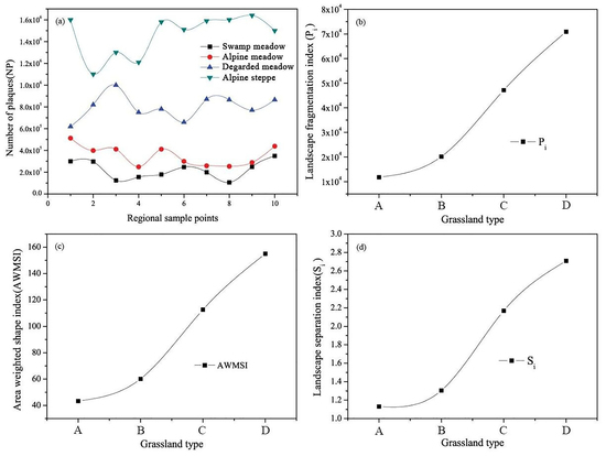
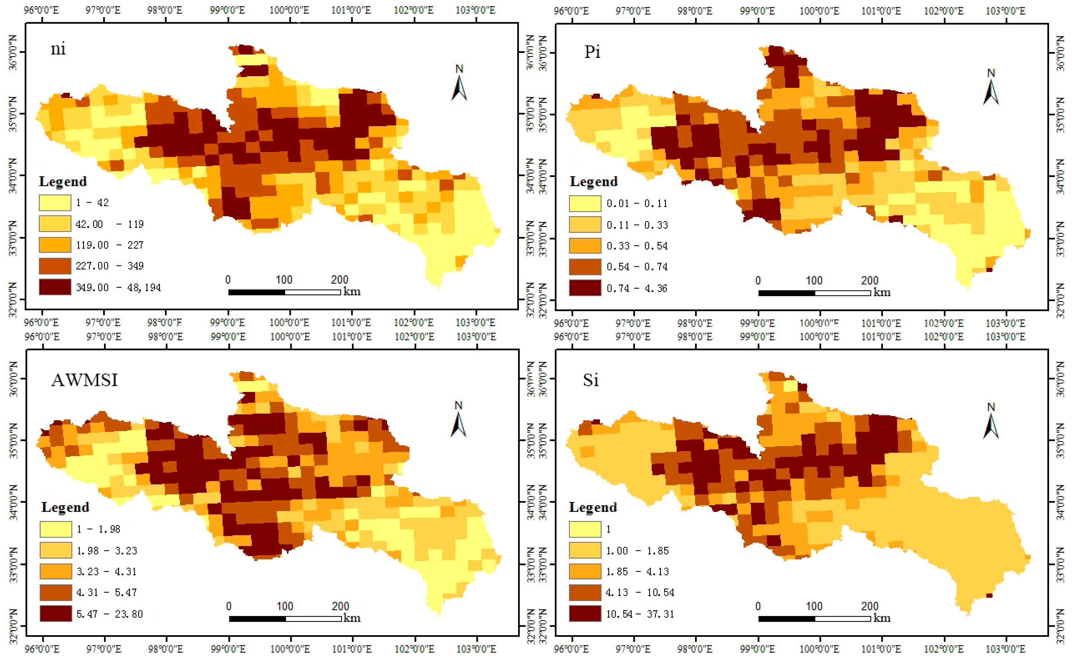
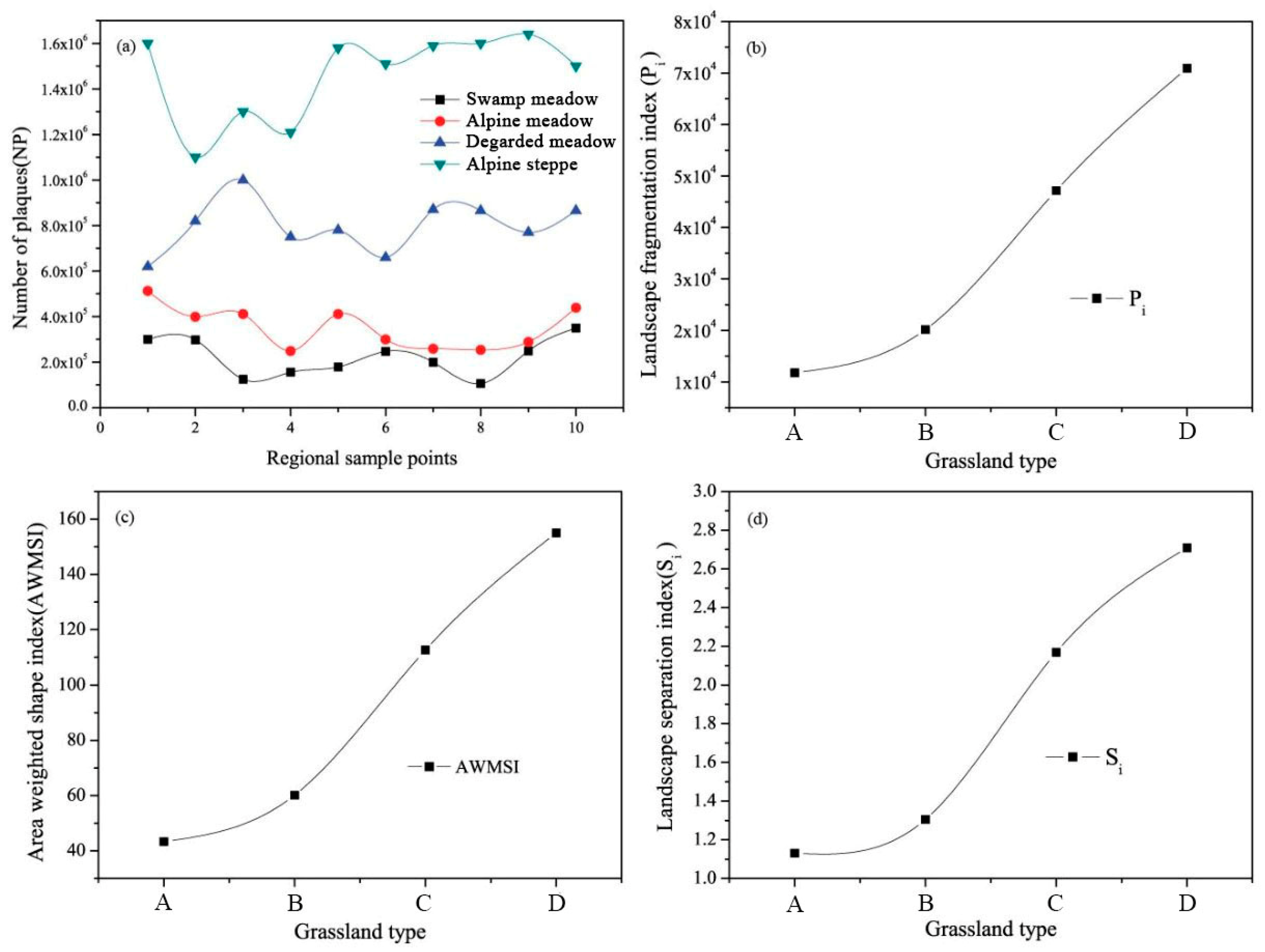
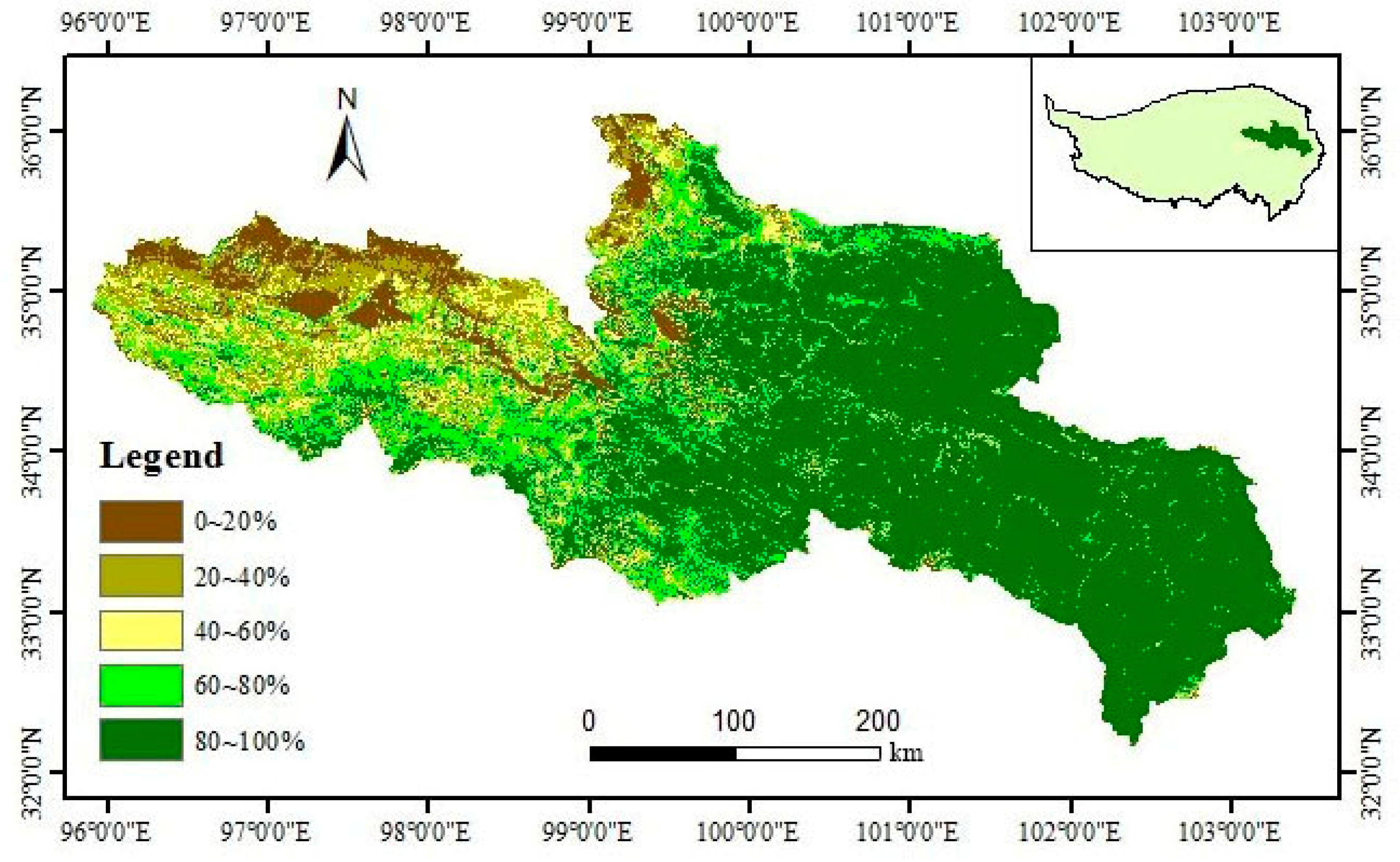
The results of the study on the patch pattern of alpine grassland in the SRYR (Figure 8) showed that the overall number of patches (n_i), fragmentation index (P_i), area-weighted shape index (AWMSI), and separation index (S_i) for the four grassland types are ordered as follows: alpine steppe > degraded meadow > alpine meadow > swamp meadow. Moreover, the greater the FVC level, the larger the landscape dominance index (DO_i), and the more complex the landscape patch pattern. Combined with landscape ecology principle, the fragmentation degree of patches is positively correlated with the number of patches. The alpine grassland and FVC levels of 60% to 80% correspond to the largest fragmentation values, indicating that this grassland type has the largest number of patches generated by ecological evolution and thus the lowest ecosystem stability. If the global climate change and livestock gradually intensified, patch fragmentation will continue to worsen, the degree of soil exposure will continue to increase [57], and the alpine grassland desertification area will gradually expand. In addition, the area weighted shape index can measure the complexity of the landscape spatial pattern. Higher values indicate more complex shapes, and it is more difficult to exchange materials, energies, and organisms with the external environment. The value of the area weighted shape index is the highest when the FVC level of grassland is 80%–100%. The area weighted index of swamp meadow is 43.355, indicating that this grassland type has the most regular shape and can promote material energy exchange, mass migration of animals and other activities. The separation index can reflect the aggregation degree between patches, and thus affects the compressive resistance between patches. When the FVC level of grassland is 40%–60%, the value is the highest (12,044.171), indicating that the landscape is the most disperse in geographical distribution and more vulnerable to external interference. The landscape dominance index can reflect the important position of patches in the landscape, and the value is the highest when the FVC level of grassland is 80%–100%, indicating that such patches can resist external interference to a greater extent, and have a better patch pattern. Many scholars used landscape indices based on landscape ecology to describe spatial structure characteristics at different scales. For example, Bautista et al. [58] found that patch metrics (such as patch number and grainsize pattern) were more suitable as explanatory variables of landscape patch pattern than patch coverage when predicted runoff and sediment yield of semi-arid landscapes based on patch level. Saura and Rubio [59] quantified the characteristics of different forest patches in the Lleida Province of Northeastern Spain based on probabilistic connectivity metric (PC) to assess the connectivity of the entire landscape ecological network. Therefore, the landscape index of quantity, fractal, and aggregation, which evolved from information theory and fractal geometry in this study, can well quantify the patch pattern related to the ecological process in the SRYR.

Patch pattern has important indicative significance to ecological risk. This study found that the patch patterns of different landscape types of ecosystems driven by nature and man-made have significant differences, which to a certain extent reflects the ecosystem’s ability to resist external disturbances [60]. Patches are affected by endogenous and induced driving forces such as altitude, temperature, geology, soil, and drought stress gradients, which will produce endogenous self-organized distribution of patches. For example, Rietkerk [61] found through predictive sequence model that with the vicious circle of global natural resources, and its catastrophic transformation of self-organized patch, depends on the degree of dominance of the initial ecosystem patch pattern. Zelnik [13] found that with the change of disturbance parameters on the Maxwell point threshold, the three trends of patch pattern are mainly perturbed by the initial disturbance degree, the greater the disturbance degree, the faster the threat to the entire ecosystem [62]. There are also scholars based on indicators and models to generate a time-series ecological model used to detect key changes in ecosystem disturbances [63]. In addition, exogenous tissue distribution can occur in patches under the influence of rodents and overgrazing. Davidson [64] studied the influence of burrowing herbivorous rodents on the vegetation community of Chihuahua Desert grassland, and found that the herbivorous and disturbance of rodents would lead to a great difference in landscape structure on spatial and temporal scales. Moreover, the overgrazing of cattle has resulted in the lack of vegetation structure resources in the agricultural ecosystem of the Sahel region of Africa [52]. Therefore, the aboveground net primary production (ANPP), root biomass, and soil nutrients in the natural environment under exogenous interference would make the energy flow and material exchange between patches more difficult [65]; thus, affect the landscape patch pattern. However, there are still uncertainties in the formation and succession mechanism of patch patterns in the SRYR, and long-term monitoring is needed to understand the driving mechanism of patch formation and development. In this study, the patch pattern represented by landscape index can well describe and predict the ability of the ecosystem to resist external interference. The larger the number (n_i, P_i), fractal (AWMSI), and the aggregation (S_i) characteristics of the patch pattern, the worse its anti-interference ability, and it will be particularly sensitive to ecological changes. The main manifestation is that the patch fragmentation shows an accelerated trend, the shape is more deviated from the regular state, and the connectivity between the patches gradually disappear.

Driven by different temperature, precipitation, topography, human activities and other factors, the patch pattern formed has a significant difference in the ability to resist external interference, which provides a protective early warning for the understanding of ecological status and catastrophic transformation of the ecosystem. Patches will gradually adapt to the ecosystem in which they are located in the process of resisting external disturbances, such as continuous degradation, succession, and ecological restoration. Some scholars have carried out researches on the adaptability of patches to ecosystems. For example, Kumar et al. [66] studied the mechanism, morphology and biochemical level of vegetation patches adapting to changes in altitude in the western Himalayas; Hesp [67] studied the adaptation pressure of coastal plants to the environment in the coastal dune environment. Therefore, different vegetation patches interact with their environmental conditions to form different patch patterns to promote ecological balance. Some vulnerable patches after external disturbance will be restored to the original ecosystem during the adaptation process. For example, Zhou et al. [57], by comparing the resilience of four grassland ecosystems in Israel and South Africa, found that the alpine meadow ecosystem has a strong resilience. Cui et al. [68] studied the vegetation restoration of typical arid and semi-arid ecosystems in the Loess Plateau of China and found that the vegetation patch pattern under the natural grassland restoration model was relatively stable under environmental stress. However, there are still certain difficulties in relying on self-recovery in ecosystems that are subject to strong external disturbances [69]. When the ecosystem shows a severe reduction of vegetation patches and the loss of the structural function of material exchange and energy exchange between the patches, the ecosystem is likely to show malignant metastasis or large-scale extinction beyond its recovery scope [70]. According to the results of this study, patches with less FVC have worse spatial pattern and are more sensitive to ecological drive. In recent years, the grassland FVC in the SRYR has been reduced due to the interference of overgrazing and rampant pika, which has a great impact on the restoration of alpine grassland.

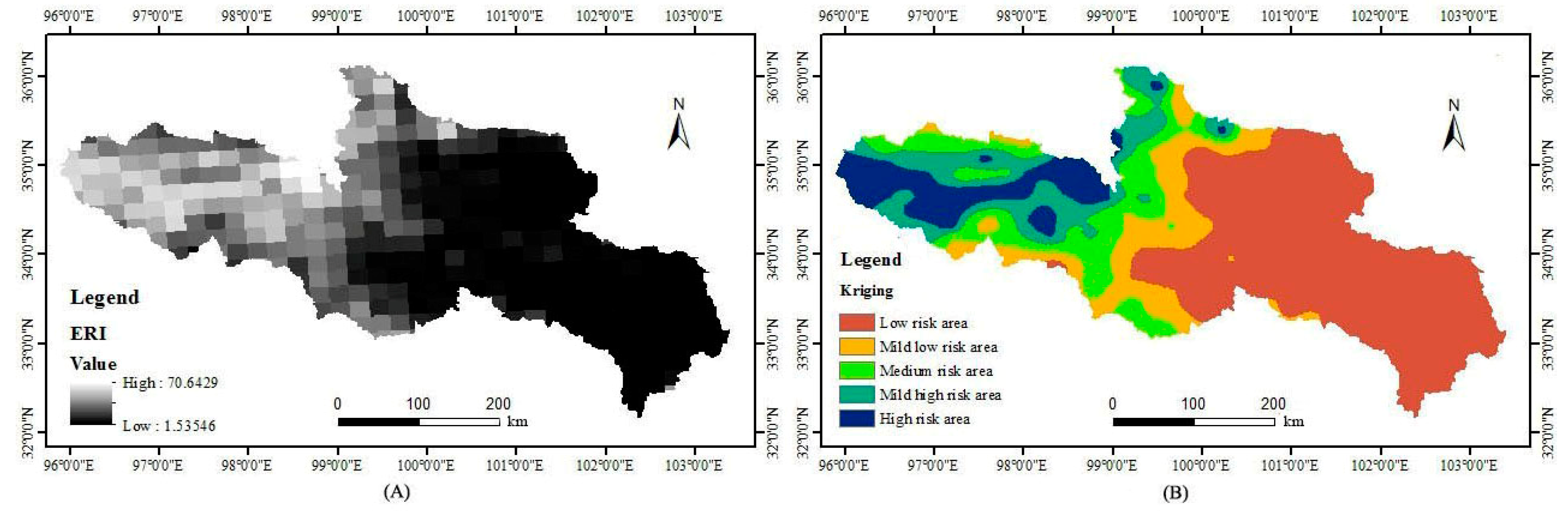
Regarding the ecological risk assessment study of the alpine grassland in the SRYR, the ecological risk index at the watershed scale is a variable that reflects the spatial pattern, and the changes in spatial structure have a certain randomness and structure [71]. Compared with the ecological risk index of site-scale, it is more capable of studying the spatial regularity and hierarchical structure of the landscape in the ecological risk spatial analysis, and it intuitively describes the spatial–temporal differentiation characteristics of ecological risk in the research area [72]. According to the results of the watershed scale and site scale, the ecological risk characteristics of alpine grassland in the eastern part of the SRYR is in the low and mild low risk area. The type of grassland is mostly swamp meadow, and the FVC is mostly 60%–80% and 80%–100%, indicating that swamp meadow is an important grassland type structure to maintain ecological stability and reduce ecological risk. Mainly because the swamp meadow grows under the conditions of over-humidity and anaerobic soil, its ecosystem is a relatively stable system formed by the driving factors of water. Moreover, it has a good patch pattern and can effectively exchange materials and information between patches. The ecological risks in the western region are in high, mild high, and medium risks. The types of grassland are mostly degraded meadow, alpine meadow, and alpine steppe, and its FVC is mostly 0–60%. This indicates that due to the influence of global warming and other factors, the grassland types in these risk areas are subject to a gradual reduction in grassland patches and FVC. Government departments should emphasize the importance of ecological planning of this type of grassland, build blue-green ecological corridors, increase the connectivity of small ecological patches, and improve ecological services.

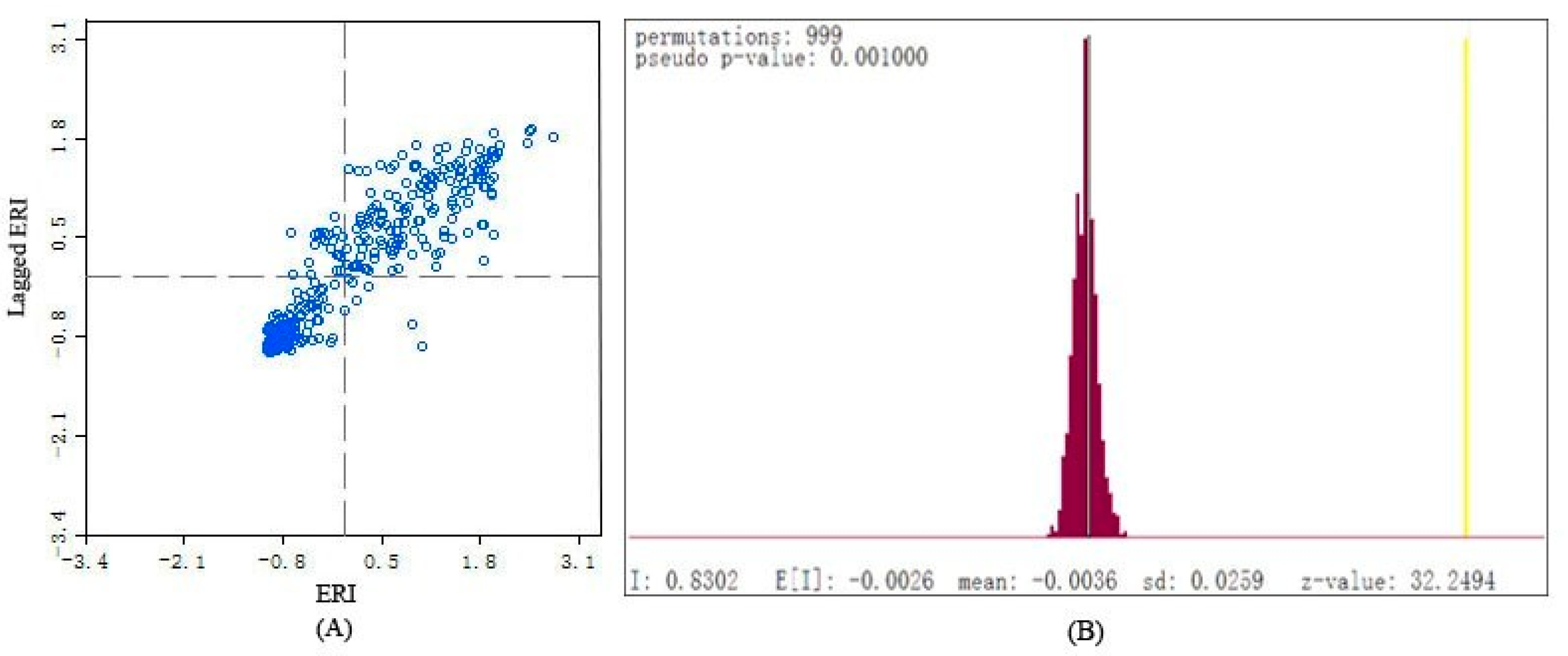
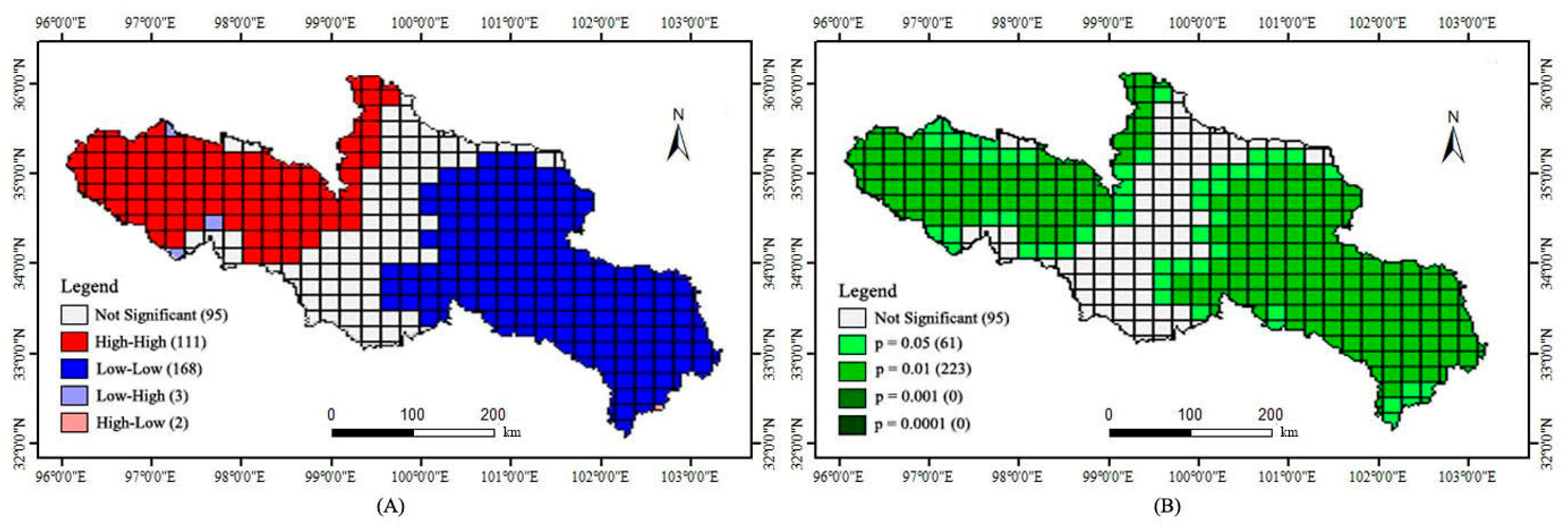
This study performed global spatial autocorrelation analysis on ecological risk by exploring the spatial correlation of ecological risk characteristics of alpine grassland in the SRYR. From this analysis, Moran’s I was 0.863 and Z = 32.249 from the random distribution test (Figure 12), which indicates that the ecological risk index has a remarkable positive correlation in space. There is mutual influence between adjacent plots, and the space tends to be homogeneous and dispersed. In addition, the standard deviation is 0.0388, which is relatively small, indicating that the fluctuation of the risk value is not significant and the overall level is stable. Since global autocorrelation analysis cannot recognize the spatial correlation of the ecological risk index between adjacent regions, local autocorrelation analysis was applied (Figure 13). LISA analysis was performed, and the results were combined with the previous research results; the high-high aggregation areas in the SRYR were mainly distributed in areas with FVC of 0–20% and 20%–40%. This showed that this region has a high ecological risk value, fragile ecological environment, and poor ecosystem stability, which aggravates the fragmentation degree of alpine grassland patches and leads to an increase in ecological risk value. The low-low aggregation area was distributed mainly in the area with FVC of 80%–100%, indicating that the area has a low ecological risk value and strong landscape connectivity. The ecological risk value of the adjacent alpine meadow with FVC of 60%–80%, which was also low. Therefore, the aggregate distribution of LISA is highly consistent with the east-west gradient spatial distribution of ecological risks and the stability of the ecosystems, and the spatial autocorrelation of patch perturbation was also explained. In addition, the high–high and low–low aggregation of the spatial autocorrelation studies is related to economic activities. For example, Ye et al. [73] studied the ecological risk spatial autocorrelation of different land use types in the Pearl River Delta, and the results showed that the high–high aggregations are distributed in core areas with high regional economic development levels and large proportions of construction, such as Guangzhou, Foshan, and Shenzhen, while the low–low aggregations are distributed in woodlands and islands with little human interference. Liu et al. [74] studied the spatial autocorrelation of ecological risks in the Honghe Basin of the Yunnan province, and found that the high-value risks were aggregated and distributed in the upper and lower riparian areas with frequent economic activities, while the low-value risks were distributed in the lower riparian areas, located in Wenshan, Xizhou, and Maguan counties. The high-risk values in this paper are aggregated in the areas with low FVC and high ecological risk where large areas of alpine meadow are distributed. The low risk values are aggregated in areas with high FVC and low ecological risk, such as shrubs and swamps. The SRYR, as a significant water source and ecological source area in China, the aggregate distribution of LISA values not only affects the ecosystem stability in the SRYR, but also has a certain regulating effect on the climate and water resources in East Asia. Therefore, in order to ensure the safety of the water for the people and to rationally develop the animal husbandry economy in the SRYR, appropriate countermeasures should be taken against the high-high and low-low aggregations analyzed by LISA.

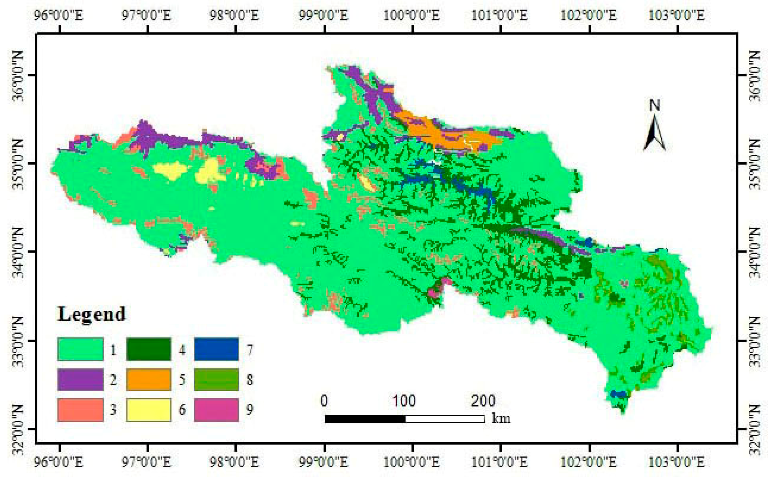
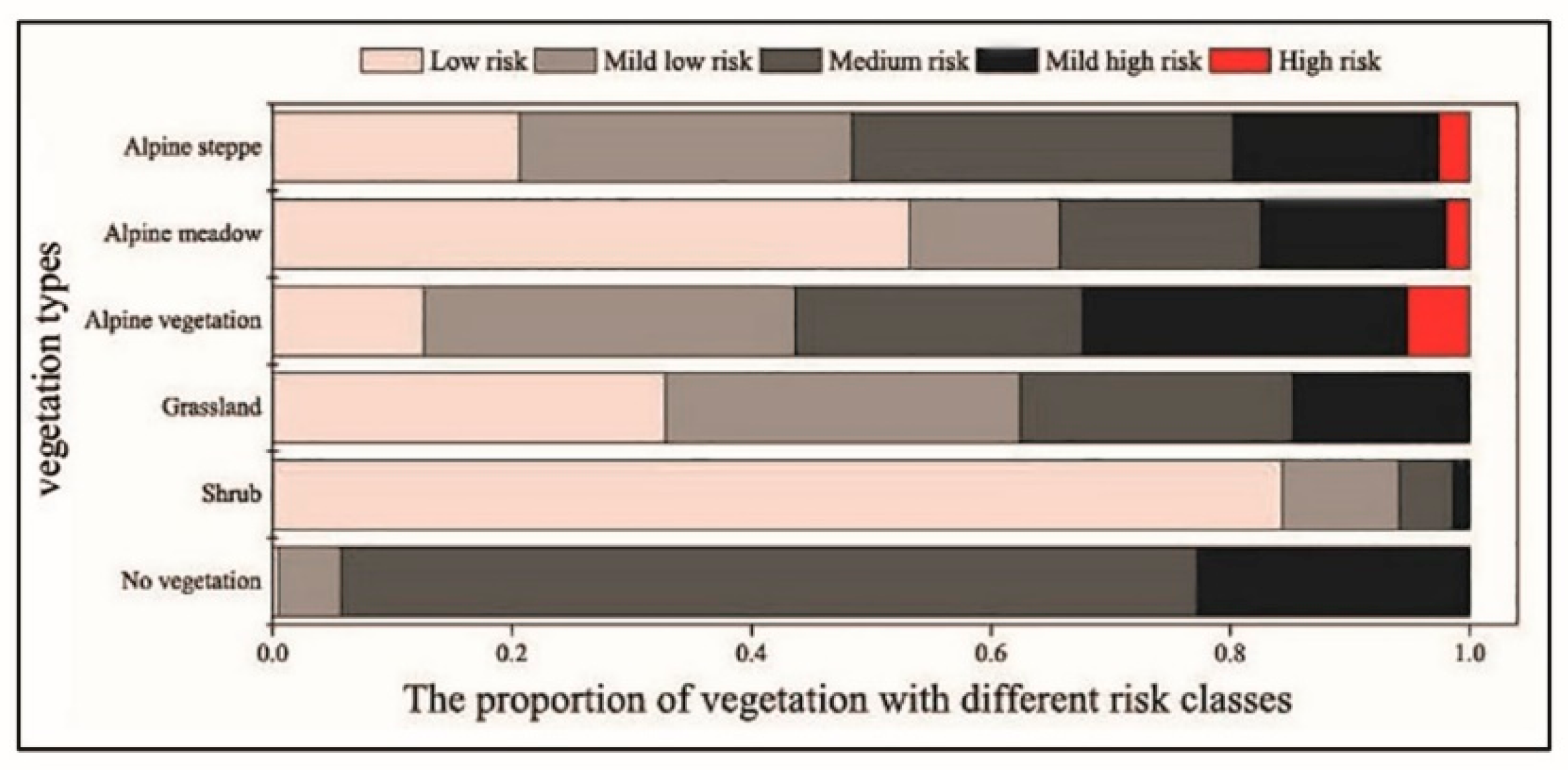
The ecological risks of different vegetation types in the SRYR (Figure 5) indicate that the area proportion of each vegetation is consistent with the study on alpine grassland patch pattern in the SRYR. The results show that there are high-risk patch distributions in the three following types: alpine vegetation, alpine steppe, and alpine meadow, which account for 3.51%, 5.05%, and 74.99% of the SRYR total area, respectively (

Table 7. Proportion of each vegetation type area to total area of the SRYR.

Vegetation Type	Percentage of the Total Area of the SRYR/%
Alpine steppe	5.05
Alpine meadow	74.99
Alpine vegetation	3.51
Grassland	1.70
Shrub	10.04
No vegetation	1.27

). Their patch fragmentation is large, FVC is small, and the overall patch pattern is complex and poorly aggregated, and great attention should be given to take protective measures for these three vegetation types, whereas only preventive measures need to be taken in other risk areas. The low-risk area is dominated by shrubs, which account for 10.04% of the SRYR total area and are mainly distributed in the eastern part of the SRYR. It should be emphasized to avoid the continual degradation of the ecosystem caused by human interference and other factors. Therefore, the characteristic distribution of ecological risk is closely bound up with landscape type. For example, Ruan et al. [75] studied the ecological risk distribution of different landscape types in Qingpu District, Shanghai. The results showed that towns are the main contributors to high-risk areas, farmland is the main contributor to medium-risk areas, and low-risk areas are dominated by wetlands and woodlands. Zhao et al. [50] studied major land use transformation and the rate that it affected ecological risk degree in the upper reaches of the Ganjiang River, and found that land use transformation leads to an increase in landscape ecological risks. The results show that there is a high ecological risk in the transformation between agriculture and forest land. In combination with the research results, the ecological risk level is the highest for landscape types with weak ecological stability and susceptibility to human disturbance. There will be different levels of ecological risks if the two landscape types are converted. Ecological protection should be increased for ecologically sensitive landscape types, and quantitative and qualitative research on the ecological risk impact factors of landscape types should be continued in future research.

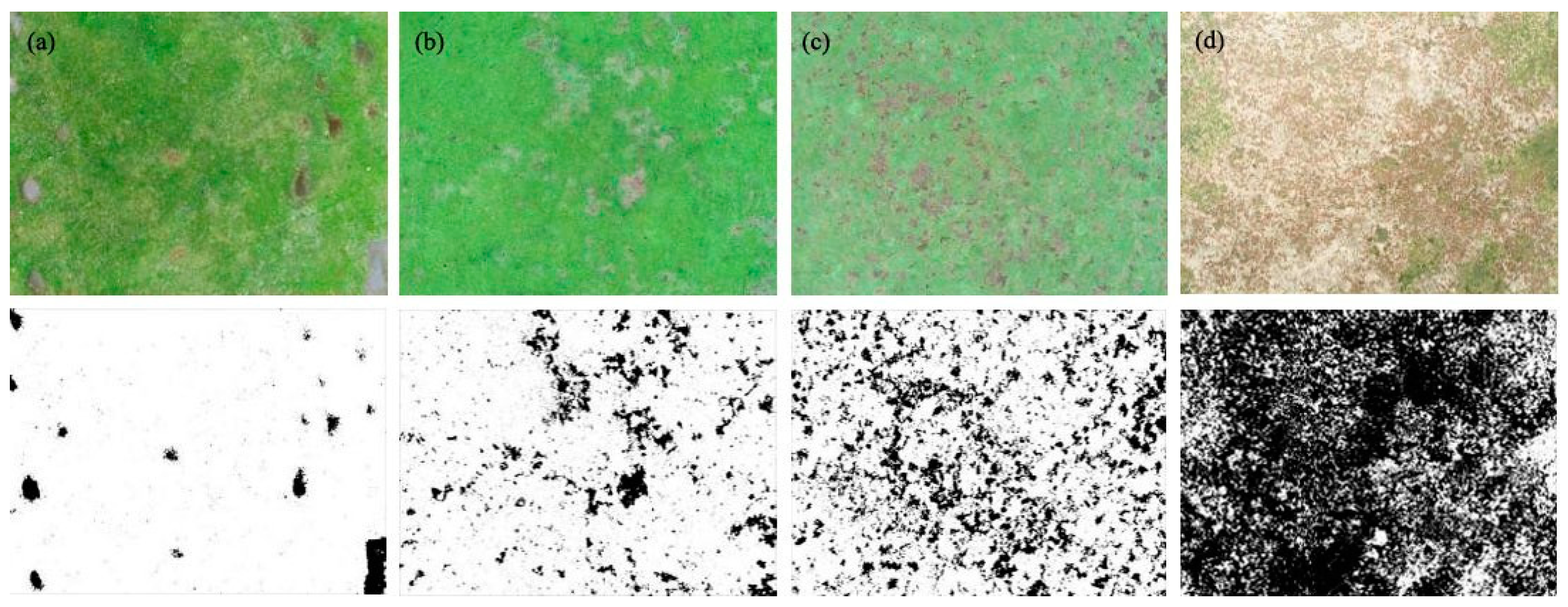
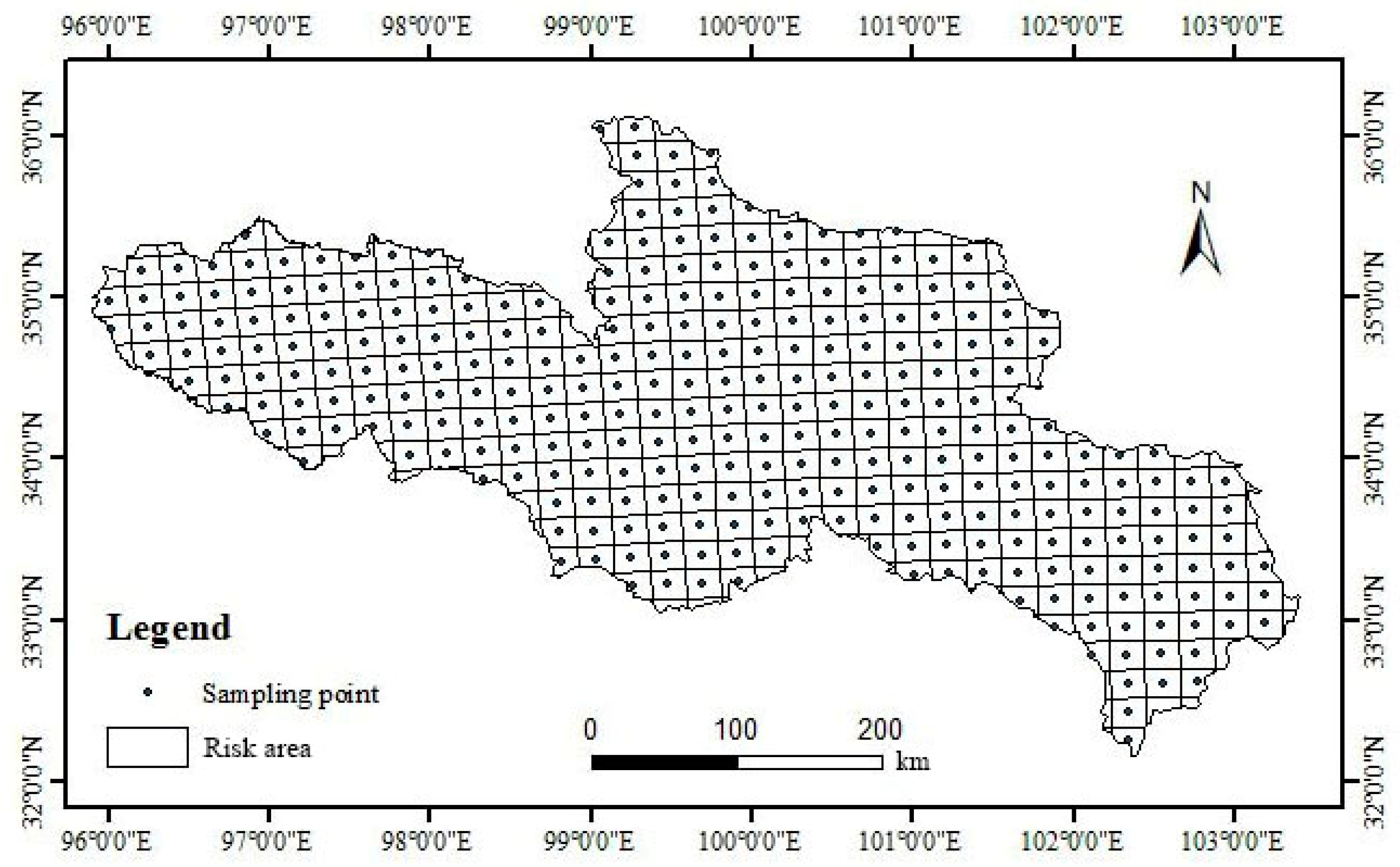
With the increasing warming of the global climate and the frequent expansion of human activities, vegetation and bare land patches in fragile ecosystems alternate in the spatial pattern [76]. Bordeu et al. [77] discovered the phenomenon of self-replication in the Festuca grassland patch through remote sensing analysis of the Andean highlands. Meng et al. [78] found that the heterogeneity of bare patch increased year by year in Changting County, Fujian Province, China. The pattern characteristics reflected by patches play an important role in understanding ecological status and processes. By exploring the patch pattern and ecological risks of alpine grasslands in the SRYR, we can take targeted protection measures for vegetation patches of different grassland types and different FVC to achieve ecosystem stability. This study used both high-resolution UAV aerial images and satellite images to analyze patch patterns and ecological risks at two scales, and it avoids the uncertainty caused by a single data. The results of this study have certain reference significance for other fragile ecosystem patch research. In addition, we have set up 417 long-term observation sites in the SRYR since 2015. For each observation site, we use UAV to monitor grassland patches during the peak season of vegetation growth every year, to study the patch changes and succession characteristics in this region. At the same time, we have installed soil water heat and air temperature and humidity measurement systems for different grassland types to provide environmental factor data for the study of patch change processes. However, the natural succession process of patches is very slow, and it is difficult to obtain ideal results in the short term. Therefore, long-term monitoring data is needed to understand and master the drivers of alpine grassland patch change and succession, which is also our long-term research goal.

5. Conclusions

Based on UAV aerial images and satellite remote sensing images, this study evaluated the patch patterns and ecological risks characteristics of alpine grassland in the SRYR at site and watershed scales using image interpretation, spatial analysis, and other methods. The results showed that the patch pattern is complex, and the patch characteristics of different grassland types are significantly different in the SRYR. The patch fragmentation, area weighted shape index, and separation degree of alpine steppe, degraded meadow, alpine meadow, and swamp meadow increased gradually, indicating that patch characteristics have good indicative significance for alpine grassland ecological protection, which should be considered in future studies. In addition, the ecological risk in the SRYR has a gradual increase from east to west. Among this, the ecological risk in the northwest region is relatively high, and the ecological risk has obvious high–high aggregation and low–low aggregation phenomena. Therefore, it is necessary to increase ecological and environmental protection in the future in order to better protect the SRYR, especially in the northwest region of the SRYR.

References

1. Giovannetti, F. A Framework for Integrating Sustainable Management Plan for Kalagala Offset into the Management Plans of the Central Forest Reserves of Mabira Ecosystem; The World Bank: Washington, DC, USA; National Forestry Authority: Kampala, Uganda, 2009; pp. 1–21.
2. Shekhawat, N.S.; Phulwaria, M.; Rai, M.K.; Kataria, V.; Shekhawat, S.; Gupta, A.K.; Rathore, N.S.; Vyas, M.; Rathore, N.; Vibha, J.B.; et al. Bioresearches of fragile ecosystem/desert. Proc. Natl. Acad. Sci. India Sect. B Biol. Sci. 2012, 82, 319–334. [Google Scholar] [CrossRef]
3. Chuvieco, E.; Aguado, I.; Yebra, M.; Nieto, H.; Salas, J.; Martín, M.P.; Vilar, L.; Martínez, J.; Martín, S.; Ibarra, P.; et al. Development of a framework for fire risk assessment using remote sensing and geographic information system technologies. Ecol. Model. 2010, 221, 46–58. [Google Scholar] [CrossRef]
4. Forman, R.T.T.; Godron, M. Patches and structural components for a landscape ecology. Bioscience 1981, 31, 733–739. [Google Scholar]
5. Forman, R.T.T.; Godron, M. Landscape Ecology; Wiley: New York, NY, USA, 1986. [Google Scholar]
6. Roughgarden, J. Patchiness in the spatial distribution of a population caused by stochastic fluctuations in resources. Oikos 1977, 29, 52–59. [Google Scholar] [CrossRef]
7. Bastin, G.N.; Ludwig, J.A.; Eager, R.W.; Chewings, V.H.; Liedloff, A.C. Indicators of landscape function: Comparing patchiness metrics using remotely-sensed data from rangelands. Ecol. Indic. 2002, 1, 247–260. [Google Scholar] [CrossRef]
8. Gustafson, E.J. Quantifying landscape spatial pattern: What is the state of the art? Ecosystems 1998, 1, 143–156. [Google Scholar] [CrossRef]
9. Pei, L.; Jia, S.J.; Han, R.M.; Zhang, H.W. Landscape Pattern and Ecological Security Assessment and Prediction Using Remote Sensing Approach. J. Sens. 2018, 2018, 1058513. [Google Scholar]
10. Fernando, M.; Nakamura, G.M.; Granzotti, C.R.F.; Martinez, A.S. Vegetation cover reveals the phase diagram of patch patterns in drylands. Phys. A Stat. Mech. Appl. 2019, 534, 122048. [Google Scholar]
11. Lavorel, S.; Grigulis, K.; Leitinger, G.; Kohler, M.; Schirpke, U.; Tappeiner, U. Historical trajectories in land use pattern and grassland ecosystem services in two European alpine landscapes. Reg. Environ. Chang. 2017, 17, 2251–2264. [Google Scholar] [CrossRef]
12. Ramachandra, T.V.; Aithal, B.H.; Sanna, D.D. Insights to urban dynamics through landscape spatial pattern analysis. Int. J. Appl. Earth Obs. Geoinf. 2012, 18, 329–343. [Google Scholar]
13. Zelnik, Y.R.; Meron, E. Regime shifts by front dynamics. Ecol. Indic. 2018, 94, 544–552. [Google Scholar] [CrossRef]
14. Wright, J.P.; Gurney, W.; Jones, C.G. Patch dynamics in a landscape modified by ecosystem engineers. Oikos 2004, 105, 336–348. [Google Scholar] [CrossRef]
15. Xu, Z.; Shen, Y.; Liao, J. Patch dynamics of various plant-animal interactions in fragmented landscapes. Ecol. Model. 2018, 368, 27–32. [Google Scholar] [CrossRef]
16. Tlidi, M.; Bordeu, I.; Clerc, M.G.; Escaff, D. Extended patchy ecosystems may increase their total biomass through self-replication. Ecol. Indic. 2018, 94, 534–543. [Google Scholar] [CrossRef] [Green Version]
17. Kefi, S.; Rietkerk, M.; Roy, M.; Franc, A.; Ruiter, P.C.; Pascual, M. Robust scaling in ecosystems and the meltdown of patch size distributions before extinction. Ecol. Lett. 2011, 14, 29–35. [Google Scholar] [CrossRef] [Green Version]
18. Liang, S.L.; Li, X.W.; Wang, J.D. Chapter 13—Fractional Vegetation Cover. Adv. Remote Sens. 2012, 9780123859549, 415–438. [Google Scholar]
19. Fu, L.T.; Bo, T.L.; Du, G.Z.; Zheng, X.J. Modeling the responses of grassland vegetation coverage to grazing disturbance in an alpine meadow. Ecol. Model. 2012, 247, 221–232. [Google Scholar] [CrossRef]
20. Peng, J.; Liu, Y.H.; Shen, H.; Han, Y.N.; Pan, Y.J. Vegetation coverage change and associated driving forces in mountain areas of Northwestern Yunnan, China using RS and GIS. Environ. Monit Assess 2012, 184, 4787–4798. [Google Scholar] [CrossRef]
21. Sun, C.Y.; Zhang, J.Q.; Ma, Q.Y.; Chen, Y.N. Human Health and Ecological Risk Assessment of 16 Polycyclic Aromatic Hydrocarbons in Drinking Source Water from a Large Mixed-Use Reservoir. Int. J. Environ. Res. Public Health 2015, 12, 13956–13969. [Google Scholar] [CrossRef] [Green Version]
22. Faber, J.H.; Van, W.J. Elaborations on the use of the ecosystem services concept for application in ecological risk assessment for soil. Sci. Total Environ. 2011, 415, 3–8. [Google Scholar] [CrossRef]
23. Loucks, O.L. Looking for surprise in managing stressed ecosystems. BioScience 1985, 35, 202–207. [Google Scholar] [CrossRef]
24. Mansour, S.; Gad, M.F. Risk assessment of pesticides and heavy metals contaminants in vegetables: A novel bioassay method using Daphnia magna Straus. Food Chem. Toxicol. 2010, 48, 377–389. [Google Scholar] [CrossRef] [PubMed]
25. Natio, W.; Miyamoto, K.; Nakanishi, J.; Masunaga, S.; Bartell, M.S. Evaluation of an ecosystem model in ecological risk assessment of chemicals. Chemosphere 2003, 53, 363–375. [Google Scholar]
26. Sciera, K.L. Quantifying the effects of land use change on stream ecosystems for use in ecological risk assessment. ProQuest LLC 2008, 333, 9416. [Google Scholar]
27. Malekmohammadi, B.; Blouchi, L.R. Ecological risk assessment of wetland ecosystems using Multi Criteria Decision Making and Geographic Information System. Ecol. Indic. 2014, 41, 133–144. [Google Scholar] [CrossRef]
28. Brown, S.S.; Reinert, K.H. Framework for ecological risk assessment. Environ. Toxicol. Chem. 1992, 11, 143–144. [Google Scholar] [CrossRef]
29. Suter, G.W.; Norton, S.B.; Barnthouse, L.W. The evolution of frameworks for ecological risk assessment from the red book ancestor. Hum. Ecol. Risk Assess. 2003, 9, 1349–1360. [Google Scholar] [CrossRef]
30. Mcdonald, L.; Mcdonald, T.L. A new ecological risk assessment procedure using resource selection models and geographic information systems. Wildl. Soc. Bull. 2002, 30, 1015–1021. [Google Scholar]
31. Thomsen, M.; Faber, J.H.; Sorensen, P.B. Soil ecosystem health and services: Evaluation of ecological indicators susceptible to chemical stressors. Ecol. Indic. 2012, 16, 67–75. [Google Scholar] [CrossRef]
32. Hakanson, L. An ecological risk index for aquatic pollution control—A sedimentological approach. Water Res. 1980, 14, 975–1001. [Google Scholar] [CrossRef]
33. Washington-Allen, R.A. Retrospective Ecological Risk Assessment of Rangeland Health Using Multitemporal Satellite Imagery. Ph.D. Thesis, Utah State University, Logan, UT, USA, 2003. [Google Scholar]
34. Barnthouse, L.; Suter, G.W.; Bartell, S.M. Quantifying risks of toxic chemicals to aquatic populations and ecosystems. Chemosphere 1988, 17, 1487–1492. [Google Scholar] [CrossRef]
35. Hunsaker, C.T.; Graham, R.L.; Suter, G.W.; O’Neill, R.V.; Barnthouse, L.W.; Gardner, R.H. Assessing ecological risk on a regional scale. Environ. Manag. 1990, 14, 325–332. [Google Scholar] [CrossRef]
36. Paukert, C.P.; Pitts, K.L.; Whittier, J.B.; Olden, J.D. Development and assessment of a landscape-scale ecological threat index for the Lower Colorado River Basin. Ecol. Indic. 2011, 11, 304–310. [Google Scholar] [CrossRef]
37. Peng, J.; Pan, Y.J.; Liu, Y.X.; Zhao, H.J. Linking ecological degradation risk to identify ecological security patterns in a rapidly urbanizing landscape. Habitat Int. 2018, 71, 110–124. [Google Scholar] [CrossRef]
38. Zhao, X.Q.; Ma, Y.S.; Zhou, H.K. Restoration and Sustainable Management of Degraded Ecosystems in the Three River Source Areas; Science Press: Beijing, China, 2011; pp. 85–126. [Google Scholar]
39. Wang, G.X.; Li, Y.S.; Wang, Y.B. Landsurface Processes and Environmental Changes River Headwater Regions of QINGHAI-TIBET Plateau; Science Press: Beijing, China, 2010; pp. 65–98. [Google Scholar]
40. Yi, S. FragMAP: A tool for long-term and cooperative monitoring and analysis of small-scale habitat fragmentation using an unmanned aerial vehicle. Int. J. Remote Sens. 2017, 38, 2686–2697. [Google Scholar] [CrossRef]
41. Yi, S.H.; Chen, J.J.; Qin, Y. Preliminary application of aerial photos using UAV on the ecological studies ofalpine grassland on Qinghai-Tibetan Plateau. J. Southwest Univ. Natl. (Nat. Sci. Ed.) 2016, 42, 1–7. [Google Scholar]
42. Chen, J.J.; Yi, S.H.; Qin, Y.; Wang, X.Y. Improving estimates of fractional vegetation cover based on UAV in alpine grassland on the Qinghai-Tibetan Plateau. Int. J. Remote Sens. 2016, 8, 1922–1936. [Google Scholar] [CrossRef]
43. Chen, J.J.; Yi, S.H.; Qin, Y. The contribution of plateau pika disturbance and erosion on patchy alpine grassland soil on the Qinghai-Tibetan Plateau: Implications for grassland restoration. Geoderma 2017, 297, 1–9. [Google Scholar] [CrossRef]
44. Chen, J.J.; Zhao, X.N.; Zhang, H.Z.; Qin, Y.; Yi, S.H. Evaluation of the accuracy of the field quadrat survey of alpine grassland fractional vegetation cover based on the satellite remote sensing pixel scale. ISPRS Int. J. Geo-Inf. 2019, 8, 497. [Google Scholar] [CrossRef] [Green Version]
45. Kun, J.; Liang, S.L.; Liu, S.H.; Li, Y.W.; Xiao, Z.Q.; Yao, Y.J.; Jiang, B.; Zhao, X.; Wang, X.X.; Xu, S.; et al. Global Land Surface Fractional Vegetation Cover Estimation Using General Regression Neural Networks from MODIS Surface Reflectance. IEEE Trans. Geosci. Remote Sens. 2015, 53, 4787–4796. [Google Scholar]
46. Wu, Z.H.; Lei, S.G.; Lu, Q.Q.; Ge, S.J. Spatial distribution of the impact of surface mining on the landscape ecological health of semi-arid grasslands. Ecol. Indic. 2019, 111, 105996. [Google Scholar] [CrossRef]
47. Cao, Q.W.; Zhang, X.W.; Lei, D.M. Multi-scenario simulation of landscape ecological risk probability to facilitate different decision-making preferences. J. Clean. Prod. 2019, 227, 325–335. [Google Scholar] [CrossRef]
48. Wendel, J.; Buttenfield, B.P.; Stanislawski, L.V. An evaluation of unsupervised and supervised learning algorithms for clustering landscape types in the United States. Cartogr. Geogr. Inf. Sci. 2016, 43, 233–249. [Google Scholar] [CrossRef]
49. Bartolo, R.E.; Dam, R.A.; Bayliss, P. Regional ecological risk assessment for Australia’s tropical rivers: Application of the relative risk model. Hum. Ecol. Risk Assess. 2012, 18, 16–46. [Google Scholar] [CrossRef]
50. Zhao, Y.; Luo, Z.J.; Li, Y. Study of the spatial-temporal variation of landscape ecological risk in the upper reaches of the Ganjiang River Basin based on the “production-living-ecological space”. Acta Ecol. Sin. 2019, 39, 4676–4686. [Google Scholar]
51. Wang, P.; Wang, Y.J.; Liu, X.P.; Kong, F.X. Ecological risk assessment of an ecological migrant resettlement region based on landscape structure: A case study of Hongsibu in Ningxia. Acta Ecol. Sin. 2018, 38, 2672–2682. [Google Scholar]
52. Hu, H.B.; Liu, H.Y.; He, J.F.; An, J. The urbanization effects on watershed landscape structure and their ecological risk assessment. Acta Ecol. Sin. 2011, 31, 3432–3440. [Google Scholar]
53. O’Neill, R.V.; Hunsaker, C.T. Scale problems in reporting landscape pat tern at the regional scale. Landsc. Ecol. 1996, 11, 169–180. [Google Scholar] [CrossRef]
54. Darand, M.; Doostkamian, M.; Rehmani, M.I.A. Spatial autocorrelation analysis of extreme precipitation in Iran. Russ. Meteorol. Hydrol. 2017, 42, 415–424. [Google Scholar] [CrossRef]
55. Cuoco, A.; Serpico, P.D.; Haugboelle, T.; Kachelriess, M.; Hannestad, S. A global autocorrelation analysis of the Auger data. Eur. Solid State Device Res. Conf. IEEE 2008, 702, 825. [Google Scholar]
56. Melecky, L. Spatial autocorrelation method for local analysis of the EU. Procedia Econ. Financ. 2015, 23, 1102–1109. [Google Scholar] [CrossRef] [Green Version]
57. Zhou, H.K.; Zhao, X.Q.; Zhao, L.; Li, Y.N.; Wang, S.P.; Xu, S.X.; Zhou, L. Restoration capability of alpine meadow ecosystem on Qinghai-Tibetan Plateau. Chin. J. Ecol. 2008, 27, 697–704. [Google Scholar]
58. Bautista, S.; Mayor, A.G.; Bourakhouadar, J.; Bellot, J. Plant Spatial Pattern Predicts Hillslope Runoff and Erosion in a Semiarid Mediterranean Landscape. Ecosystems 2007, 10, 987–998. [Google Scholar] [CrossRef] [Green Version]
59. Saura, S.; Rubio, L. A common currency for the different ways in which patches and links can contribute to habitat availability and connectivity in the landscape. Ecography 2010, 33, 523–537. [Google Scholar] [CrossRef]
60. Maestre, F.T.; Escudero, A. Is the patch size distribution of vegetation a suitable indicator of desertification processes? Ecology 2009, 90, 1729–1735. [Google Scholar] [CrossRef]
61. Rietkerk, M.; Dekker, S.C.; Ruiter, P.C.; Koppel, J. Self-Organized Patchiness and Catastrophic. Science 2004, 305, 1926–1929. [Google Scholar] [CrossRef] [Green Version]
62. Zelnik, Y.R.; Meron, E.; Bel, G. Gradual regime shifts in fairy circles. Proc. Natl. Acad. Sci. USA 2015, 112, 12327–12331. [Google Scholar] [CrossRef] [Green Version]
63. Dakos, V.; Carpenter, S.R.; Brock, W.A.; Ellison, A.M.; Guttal, V.; Rlves, A.; Kefi, S.; Livina, V.; Seekell, D.A.; Vannes, E.H.; et al. Methods for Detecting Early Warnings of Critical Transitions in Time Series Illustrated Using Simulated Ecological Data. PLoS ONE 2012, 7, e41010. [Google Scholar] [CrossRef] [Green Version]
64. Davidson, A.D.; Lightfoot, D.C. Burrowing rodents increase landscape heterogeneity in a desert grassland. J. Arid Environ. 2008, 72, 1133–1145. [Google Scholar] [CrossRef]
65. Milchunas, D.G.; Lauenroth, W.K. Quantitative Effects of Grazing on Vegetation and Soils over a Global Range of Environments. Ecol. Monogr. 1993, 63, 327–366. [Google Scholar] [CrossRef]
66. Kumar, S.; Vats, S.K. Plant adaptation in mountain ecosystem. In Plant Biotechnology: Principles and Applications; Abdin, M., Kiran, U., Kamaluddin Ali, A., Eds.; Springer: Singapore, 2017. [Google Scholar]
67. Hesp, P.A. Ecological processes and plant adaptations on coastal dunes. J. Arid Environ. 1991, 21, 165–191. [Google Scholar] [CrossRef]
68. Cui, Y.X.; Linchuan Fang, L.C.; Guo, X.B.; Han, F.; Ju, W.L.; Ye, L.P.; Wang, X.; Tan, W.F.; Zhang, X.C. Natural grassland as the optimal pattern of vegetation restoration in arid and semi-arid regions: Evidence from nutrient limitation of soil microbes. Sci. Total Environ. 2018, 648, 388–397. [Google Scholar] [CrossRef] [PubMed]
69. Brandner, J.; Auerswald, K.; Cerwenka, A.F.; Schliewen, U.K.; Geist, J. Comparative feeding ecology of invasive Ponto-Caspian gobies. Hydrobiologia 2013, 703, 113–131. [Google Scholar] [CrossRef]
70. Fischer, J.; Lindenmayer, D.B. Landscape modification and habitat fragmentation: A synthesis. Global Ecol. Biogeogr. 2007, 16, 265–280. [Google Scholar] [CrossRef]
71. Mcdaniels, T.; Axelrod, L.J.; Slovic, P. Characterizing perception of ecological risk. Risk Anal. 1995, 15, 575–588. [Google Scholar] [CrossRef] [Green Version]
72. Olivera, M.A.; Webster, R. A tutorial guide to geostatistics: Computing and modelling variograms and Kriging. Catena 2014, 113, 56–69. [Google Scholar] [CrossRef]
73. Ye, C.S.; Feng, Y.F. Ecological risk assessment for Pearl River Delta based on land use change. Trans. Chin. Soc. Agric. Eng. 2013, 29, 224–232. [Google Scholar]
74. Liu, S.L.; Liu, Q.; Zhang, Z.L. Landscape ecological risk and driving force analysis in Red river Basin. Acta Ecol. Sin. 2014, 34, 3728–3734. [Google Scholar]
75. Ruan, J.J.; Wang, M.; Wang, H.Y. Regional Ecological Risk Assessment Based on Landscape Pattern: A Case Study in Qingpu District of Shanghai City. Shanghai Environ. Sci. 2016, 35, 47–52. [Google Scholar]
76. Noy-Meir, I. Desert ecosystems: Environment and producers. Annu. Rev. Ecol. Syst. 1973, 4, 25–52. [Google Scholar] [CrossRef]
77. Bordeu, I.; Clerc, M.; Couteron, P.; Lefever, R.; Tlidi, M. Self-Replication of Localized Vegetation Patches in Scarce Environments. Sci. Rep. 2016, 6, 33703. [Google Scholar] [CrossRef] [PubMed] [Green Version]
78. Meng, Y.Y.; Liu, X.M.; Wu, L.; Liu, M.L.; Zhang, B.Y.; Zhao, S. Spatio-temporal variation indicators for landscape structure dynamics monitoring using dense normalized difference vegetation index time series. Ecol. Indic. 2019, 107, 105607. [Google Scholar] [CrossRef]
Figure 1. Overview of the source region of the Yellow River (SRYR).
Remotesensing 12 03460 g001
Figure 2. Unmanned aerial vehicle (UAV) field route setting.
Remotesensing 12 03460 g002
Figure 3. Spatial distribution of vegetation types (1 is alpine meadow; 2 is alpine steppe; 3 is alpine vegetation; 4 is shrub; 5 is grassland; 6 is non-vegetated area; 7 is coniferous forest; 8 is swamp; 9 is desert).
Remotesensing 12 03460 g003
Figure 4. Vegetation patch extraction software interface.
Remotesensing 12 03460 g004
Figure 5. Regional division of ecological risk plots.
Remotesensing 12 03460 g005
Figure 6. Patch extraction results of four grass types (a) swamp meadow; (b) alpine meadow; (c) degraded meadow; (d) alpine steppe.
Remotesensing 12 03460 g006
Figure 7. Hierarchical map of fractional vegetation cover (FVC) in the SRYR.
Remotesensing 12 03460 g007
Figure 8. Distribution of landscape index in the SRYR.
Remotesensing 12 03460 g008
Figure 9. Patch characteristics of four grassland types ((a) patch quantity characteristics; (b) patch fragmentation characteristics; (c) patch fractal characteristics; (d) patch aggregation characteristics, A: swamp meadow; B: alpine meadow; C: degraded meadow; D: alpine steppe).
Remotesensing 12 03460 g009
Figure 10. Spatial distribution of ecological risks in the SRYR (A) Raster distribution map of ecological risk; (B) Kriging interpolation distribution map of ecological risk.
Remotesensing 12 03460 g010
Figure 11. Proportion of ecological risk area of vegetation.
Remotesensing 12 03460 g011
Figure 12. Global autocorrelation analysis of ecological risk (A) Moran’s I scatter distribution; (B) Moran’s I random distribution test results.
Remotesensing 12 03460 g012
Figure 13. Local autocorrelation analysis of ecological risks (A) spatial distribution characteristics of local indicators (LISA) index; (B) spatial weight distribution of LISA index.
Remotesensing 12 03460 g013