Drought Stress Detection in Juvenile Oilseed Rape Using Hyperspectral Imaging with a Focus on Spectra Variability


1
Crop Research Institute Prague-Ruzyně, Division of Crop Management Systems, Drnovská 507/73, CZ161 06 Praha 6 Ruzyně, Czech Republic
2
Crop Research Institute Prague-Ruzyně, Division of Crop Protection and Plant Health, Drnovská 507/73, CZ161 06 Praha 6 Ruzyně, Czech Republic
*
Author to whom correspondence should be addressed.
Remote Sens. 2020, 12(20), 3462; https://0-doi-org.brum.beds.ac.uk/10.3390/rs12203462
Submission received: 8 September 2020
/
Revised: 5 October 2020
/
Accepted: 16 October 2020
/
Published: 21 October 2020
(This article belongs to the Special Issue Spectroscopic Analysis of Plants and Vegetation)
Abstract
:Hyperspectral imaging (HSI) has been gaining recognition as a promising proximal and remote sensing technique for crop drought stress detection. A modelling approach accounting for the treatment effects on the stress indicators’ standard deviations was applied to proximal images of oilseed rape—a crop subjected to various HSI studies, with the exception of drought. The aim of the present study was to determine the spectral responses of two cultivars, ‘Cadeli’ and ‘Viking’, representing distinctive water management strategies, to three types of watering regimes. Hyperspectral data cubes were acquired at the leaf level using a 2D frame camera. The influence of the experimental factors on the extent of leaf discolorations, vegetation index values, and principal component scores was investigated using Bayesian linear models. Clear treatment effects were obtained primarily for the vegetation indexes with respect to the watering regimes. The mean values of RGI, MTCI, RNDVI, and GI responded to the difference between the well-watered and water-deprived plants. The RGI index excelled among them in terms of effect strengths, which amounted to and units for each cultivar. A consistent increase in the multiple index standard deviations, especially RGI, PSRI, TCARI, and TCARI/OSAVI, was associated with worsening of the hydric regime. These increases were captured not only for the dry treatment but also for the plants subjected to regeneration after a drought episode, particularly by PSRI (a multiplicative effect of for ‘Cadeli’). This result suggests a higher sensitivity of the vegetation index variability measures relative to the means in the context of the oilseed rape drought stress diagnosis and justifies the application of HSI to capture these effects. RGI is an index deserving additional scrutiny in future studies, as both its mean and standard deviation were affected by the watering regimes.
1. Introduction
Given the continuing increases in average temperatures [1] and projections of more frequent and severe droughts in agricultural regions [2,3], water deficiency has been among the most extensively studied crop stress factors [4]. In pot experiments, crop responses to drought can be investigated by varying the watering regime and comparing the obtained plant reactions across the treatments [5,6,7,8]. An alternative approach is to exploit the variability of water management strategies exhibited by individual genotypes [9,10].
Several dehydration avoidance mechanisms have been described in crops [11,12]. Plants can rapidly respond to a water deficit by closing their stomata, which reduces the leaf transpiration. As a trade-off, this reduction leads to a simultaneous decrease in the photosynthesis rate, related to limited CO2 assimilation [13,14]. Differentiation of crop cultivars with respect to their stomatal conductance regulation has been proposed. Plants that manage their water resources in a conservative way and maintain a steady CO2 fixation rate, affected by moisture availability to a limited extent, have been termed as water-savers. Water-spenders, on the other hand, maximise their CO2 assimilation, depleting the available water resources at the onset of a drought due to a delayed closure of the stomata [15,16]. Cultivars with a high baseline stomatal conductance tend to not exhibit a mid-day depression in photosynthetic rates. They are capable of sustaining a high photosynthesis rate and can avoid heat stress due to the cooling action of the transpiration, provided that water is available [17].
Stressed and healthy vegetation differ with respect to their spectral reflectances, with the effects of stress detectable before they become apparent to the naked eye [18,19,20]. The visible spectral region is affected by stress-induced changes in pigment concentrations and activities. These changes include anthocyanin and (relative) carotenoid accumulation aimed at protecting the photosynthetic apparatus and pigment breakdown, which accompanies chloroplast deterioration caused by oxidative stress [13,21,22,23]. As leaf mesophyll cells lose their turgor and shrink, there can be a temporary increase in the near-infrared reflectance, eventually followed by a decrease below the normal level [19]. The red-edge shifts towards shorter wavelengths and becomes less steep [20,24,25].
Among the spectral methods, imaging spectrometry (hyperspectral imaging) has been gaining recognition as a promising proximal and remote sensing technique for crop status assessment [26,27,28]. Its important advantage over the more traditional point spectrometry is the availability of precise spatial information [26], which can address the mixed spectra problem in close-range applications. This advantage is accomplished by using spectral segmentation methods [29], which enable the separation of the object and background pixels [30], or the identification of pixels affected by unfavourable illumination effects [6]. Furthermore, the presence and distribution of geometric features can be analysed in the image [29,31].
Studies devoted to drought effects on crop hyperspectra have been primarily focused on the species that dominate the global commodity market. Those species include maize [6,30] and other staple cereals [7,32,33]. A relatively large amount of attention has also been given to fruit crops [18,34,35]. On the other hand, numerous other species have so far been largely neglected by the studies, including those of regional importance.
Due to its nutritional [22,36,37] and technical [37,38] value, oilseed rape (Brassica napus L.; hereafter, OSR) is an important crop in many parts of the world. It is widespread in North America [39,40], China [40], Europe [39], and India [41]. OSR is susceptible to drought [12,22] and, along with other brassicas, the future cultivation of this species is endangered by dry spells [39,42].
The reproductive phase of OSR has been associated with an especially high sensitivity [22,43], but it can also be permanently affected by water deprivation earlier in its development. This possibility justifies extending studies to juvenile plants and to crop recovery after conclusion of the drought period, which is an underexplored research area [5]. Müller et al. [44] compared the physiological status of OSR plants that had been water-deprived at the shooting developmental stage and then rewatered with specimens receiving irrigation for the entire duration of the experiment. The treated plants exhibited reduced productivity and their physiological profiles were affected. The physiological changes in even younger plants were studied by Kosová et al. [45] and Urban et al. [15].
In addition to the physiological parameters, a trace of a drought episode can be detectable in a spectral signature of the affected crop. Such a possibility was demonstrated by Linke et al. [8] for wheat and by Sun et al. [5] for maize. The authors tested the changes of several vegetation indexes in plants exposed to repeated drought and recovery cycles. They observed a full recovery after the first cycle, but the second recovery was incomplete. As a possible cause, the authors suspected progressing cell deterioration due to oxygen radicals, which could not be neutralised in the absence of carotenoids due to their removal in the course of the preceding stress episode.
OSR has been the subject of various hyperspectral imaging studies. Based on field experiments, Piekarczyk et al. [46] and Zhang and He [47] attempted to predict its yield using vegetation indexes and partial least squares regression, respectively. Kumar et al. [41] cite several publications devoted to OSR pests and diseases. Xia et al. [37] analysed the imagery of water-logged plants. The effects of herbicide exposure were studied by Kong et al. [48]. In contrast to these stress factors, the possibilities of capturing the OSR response to drought using a hyperspectral camera remain unaddressed.
As highlighted by Kruschke and Liddell [49], “stressors […] can increase the variance of a group because not everyone responds the same way to the stressor”. In the context of close-range crop hyperspectral imaging, the “group” can refer to plant foliage or leaf tissue composed of individual leaves and cells, respectively, each responding to the change in the environment in a distinct way. Especially characteristic for stress-induced leaf senescence is the source–sink differentiation between the older and younger leaves [23]. The potential of imaging spectrometry to provide an insight into the spatial variation of stress symptoms across crop foliage was demonstrated for drought [7,32,33,50], nitrogen deficiency [51], pest infestation [50], and herbicide exposure [48]. OSR is characterised by relatively large leaves, even in early developmental phases. Hyperspectral imaging that captures leaf-level spectral variation may, therefore, prove to be a suitable approach for water deficiency detection in this crop [32].
Studies on crop responses to stress conditions frequently employ traditional experimental designs, such as a randomised block design, coupled with linear modelling for statistical inference [42,43,52]. The frequentist approach prevails in the fitting and evaluation of these models. Various authors noted the shortcomings of the frequentist statistics, and have advocated Bayesian methods as an alternative [49,53,54]. Historically, first the lack and then the high computational demands of suitable numerical methods posed obstacles towards a wider adoption of the Bayesian paradigm [55]. These hindrances have been largely removed by an increase in computer speeds [55,56], followed by improved accessibility of parallel computing [57], and the availability of software with capabilities suited to the needs of the scientific community [55,58,59,60].
One major appeal of Bayesian statistics is the ease with which interval estimates of model parameters can be quantified, even for complex models. Notably, it is possible to obtain estimates with respect to not only the mean values but also standard deviations, shape factors, or hurdle values—again, also for complex models [49]. In the context of stress detection with imaging spectroscopy, this capability can be readily exploited to assess the influence of the stressor on the spectral variation across the foliage of the affected plant.
The aim of the present study is to determine the spectral response of juvenile OSR representing two water management strategies to three types of watering regimes. The study is performed at the leaf level by employing a high-resolution hyperspectral camera. The influence of the OSR cultivars and watering regimes on the extent of leaf discolourations, vegetation indexes, and principal component scores are investigated. Bayesian statistics are used to obtain the interval estimates of the treatment effects with respect to the mean value and standard deviation differences.
2. Material and Methods
2.1. Plant Material and Experimental Factors
The experiment was based on winter OSR plants of the ‘Cadeli’ and ‘Viking’ cultivars. The two genotypes differ in terms of their drought-coping strategies, with ‘Cadeli’ representing the “water-saver strategy” and ‘Viking’ exhibiting the “water-spender strategy”, as revealed by their physiological [15,45] and proteomic [15] profiles. This difference is related to the origin of the cultivars, which is France for ‘Cadeli’ and Germany for ‘Viking’ [15].
The study was conducted on the premises of the Crop Research Institute in Prague-Ruzyně (Czech Republic). The seeds of both cultivars were obtained from OSEVA PRO s.r.o. (Opava, Czech Republic). Each seed was started on 11th May 2018 by placing it in a thermostat (Biological thermostat BT-120, Laboratorní přístroje Praha, Prague, Czechoslovakia) for two days set to 20 . The obtained seedlings were transplanted three days later to 14- diameter pots filled with of potting mixture produced at the site. The seeds were topped with an additional of the mixture. Each pot contained five seedlings of either of the cultivars. The potted plants were grown in a growth chamber (T-64, Tyler, Budapest, Hungary) in 18 –20 , under a 16- photo period, exposed to 400 // irradiance up to the second leaf (BBCH 12) developmental stage. At that point, the watering regime experimental factor was introduced.
The watering of the pots followed one of the three treatments: The control pots were watered daily to 70% of the substrate water capacity (SWC). For the pots in the dry treatment, the watering was reduced to 45% of the SWC, starting 14 days after the sowing, and 10 more days later the watering was stopped completely. The pots in the rewatered treatment were treated according to the same plan as the water-deprived plants, but after 5 days of suspended watering they were watered to 100% of the SWC to induct regeneration. The pots were grouped in the growth chamber according to the watering regime, which resulted in a lack of true replication of this factor.
A total of pots were used in the study. Table 1 depicts the pot numbers according to the two experimental factors. The uneven numbers across the treatment combinations stem from the fact that the material was used in another experiment, which involved destructive sampling.
2.2. Image Acquisition and Pre-processing
The imaging took place on 27 June 2018. By that time, the plants had attained the phase of 3 to 4 leaves (BBCH 13, 14), and pigmentation changes due to water deprivation were apparent (Figure 1a). The images were collected between 14:45 and 15:45, outdoors, in natural light conditions. The illumination was variable, as illustrated by the radiant exposure measurements from a meteorological station located at the site (Figure 2), and there were periods of no direct sunlight. A photo tent was used to obtain diffuse illumination and create a wind barrier.
The imager was a 2D frame hyperspectral camera (Rikola, Senop, Oulu, Finland), mounted on a tripod at the tent entrance (Figure 1b). An irradiance sensor was placed inside the tent to account for the variation in the illumination conditions. Its readings, expressed in relative units, varied between 82 and 181 (Figure 2), reflecting the unstable light conditions during the campaign. A dark reference was obtained prior to the acquisition of the OSR images with the aid of a 50- black masking tape (T743-2.0, Thorlabs Inc., Newton, NJ, USA). Four pots—two per cultivar and placed at the tent bottom in an alternated manner against a background of black non-woven textile—were captured in each image. Since the number of pots in the rewatered treatment was not divisible by four, some of the pots were captured for a second time. Those extra pot images were not included in the analysed dataset. First, the dry plants were imaged, followed by the watered plants, and then followed by the rewatered plants. This ordering reflected the pot grouping in the growth chamber. The images of the plants were interleaved with images of Spectralon tiles with 2, 9, 23, 44, and 75% reflectance factors. The internal camera temperature was stable, in the 32.56 –33.81 range.
The hyperspectral data cubes comprised 41 evenly spaced bands ranging from 503 to 903 . The spatial resolution was 1010 × 1010 pixels and the radiometric resolution was 12 bits. The integration time was set to 30 . The pot rims were approximately away from the camera lens, resulting in a GSD of approximately per image pixel.
Figure 3 depicts the imagery pre-processing and processing workflow. After the conversion from the digital numbers, Spectralon radiance values were sampled on a 20 × 20 pixel grid. The grid sampling was intended to reduce the effect of spatial autocorrelation and the computation time. For every band, a mixed-effect empirical line model [61] was fitted with a reflectance logit as the dependent variable, radiance as the independent variable, and pixel as the grouping variable (fit ELM in Figure 3). The logit transformation accounted for the reflectance values being constrained between 0 and 100% [62], and the grouping variable was introduced for the possibility of an uneven illumination of the scene during the acquisition process. A transformation of the radiance values to the reflectance values was performed by applying the obtained models to the individual spectral bands (pred ELM).
In the next pre-processing step, the reflectance images were subjected to band registration (reg) to remove the effect of camera sensor misalignment [63]. The ORB algorithm was used for feature detection and description and was coupled with brute-force descriptor matching [64]. The band registration failed for one of the images of the rewatered plants, probably because of leaf movements from the wind. That image was excluded from the subsequent analyses (Table 1).
In each of the plant images, the coordinates of three points along each pot circumference were identified by hand. From these, the pot centre coordinates and radii were derived. The radii lengths were then reduced by a factor of 0.95 to exclude the pot rims from the regions of interest, which were delimited as inscribed squares (crop).
2.3. Pixel Classification and Evaluation of Class Size Proportions
A random sample of 200 pixels was drawn from across all regions of interest to train and validate a classification model aimed at distinguishing between healthy (fresh) leaf zones and those exhibiting discolouration, which was attributed to drought. Due to an uneven number of pixels across the pot images, stratified sampling was employed. First, a pot was sampled, followed by a pixel within. The sampled pixels were subsequently hand-classified as either background, fresh-leaf, dry-leaf, or edge pixel, based on pseudo-RGB (R: 647 , G: 563 , B: 503 ) rendering of the pot images (Figure 1c).
The pixels at the leaf edges or zone boundaries were treated as missing data and dropped. The reflectance spectra of the remaining pixels () were randomly partitioned into the training and test dataset at a 3:1 proportion. The partitioning was stratified with respect to the pixel class. Using the training dataset, a Support Vector Machine (SVM) classification model with the radial basis function kernel [65] was fitted to the pixel hyperspectra (fit SVM). The cost hyperparameter of the model was tuned to maximise the classification accuracy using 10-fold cross-validation and the Bayesian model-based optimisation search algorithm [66]. The performance of the obtained model was then assessed using the test dataset. Finally, the model was applied to classify every pixel in the pot images (pred SVM).
The dry-leaf and fresh-leaf classes were merged to create plant masks [67], which were subsequently subjected to 3-pixel erosion [63] to remove leaf pedicels and artefacts resulting from imperfect band registration. The eroded masks were then applied to the pot images (mask).
Dry-leaf pixels were counted in each masked pot image, and the effects of the experimental treatments on the dry-leaf pixel proportion were assessed using a Bayesian linear mixed-effect model (fit LM1). The model assumed a zero-inflated binomial data generating distribution of the response variable (with a logit link) and accounted for the grouping of the leaf pixels within the pots and of the pots within the individual images. In addition to reflecting the dataset structure, the inclusion of the grouping variables was intended to address the problem of variable illumination conditions during the hyperspectral data acquisition campaign. Conservative, yet meaningful priors [54,68] were assumed.
2.4. Vegetation Index and Full-Spectrum Analyses
Twenty vegetation-index values (Table 2) were calculated for each pixel of the masked pot images (vegind). In cases where the wavelengths present in an index definition did not match the available image wavelengths, the closest wavelength was used, instead.
From each vegetation index pot image, 36 pixels were sampled on a regular grid to reduce the effect of spatial correlation while retaining information on the within-pot index value variation. Pixels located in the masked-out areas were discarded. To assess the effect of the experimental treatments on the index values, an ensemble of univariate Bayesian linear mixed-effect models was fitted (fit LM2). The individual model formulations took the sample–pot–image grouping hierarchy of the observations into account and relaxed the assumption of index value homoscedasticity across the treatment combinations. Because of the variety of the indexes, the modelling assumed uninformative priors [55,84].
In addition to the vegetation-index approach, an analysis based on the full-spectrum information from raw and pre-processed spectra was attempted. The pre-processing scenarios (trans) comprised the Savitzky–Golay filter (SGF), multiplicative scatter correction (MSC), finite differences derivation, and second derivation [85]. In the next step, the spectra were subjected to dimensionality reduction using PCA to remove redundant radiometric information. The influence of the experimental treatments on the first four PCA loading values was then assessed using multivariate linear modelling (fit LM3), readily available in the Bayesian paradigm [55], to take the correlations between the loadings into account. The predictor part of the model was formulated in the same way as for the vegetation indexes.
2.5. Statistical Inference and Model Diagnostics
Accuracy of the SVM classification was determined using a confusion matrix. For the linear models, the posterior distributions of parameters were derived and visualised to assess the directions, magnitudes, and uncertainties of treatment effect estimates. Numerical summaries: posterior mode and a 95% credibility interval [49,54] were also computed. The estimated differences among the vegetation index means were additionally converted to Cohen’s d relative effect sizes, with the watered treatment index standard deviations pooled across the cultivars as the standardiser [86]. The fits of the linear models were assessed using the R-hat statistics [59], by inspecting posterior trace plots [55], and performing predictive posterior checks [54].
2.6. Reproducing the Study
Pre-processed hyperspectral data cubes are available from a Zenodo repository along with the scripts that were employed for their analysis (doi:10.5281/zenodo.3975431). A GNU Guix [87] manifest file and definitions of extra software packages are also included to recreate the computational environment. A Makefile [88] describes and facilitates the execution of individual steps of data processing.
A major part of the analysis was programmed in the R language, and run in the 3.6.1 version of the interpreter [89]. The e1071 package (version 1.7.2) [90] was employed to fit the SVM model, and mlr (2.15.0) [91] was used in combination with mlrMBO (1.1.2) [66] for its tuning. The Bayesian linear models were fitted with the aid of the brms (2.10.0) [58] interface to Stan (2.19.1) [59]. Tools available in SAGA GIS (6.3.0) [92], accessed from the RSAGA package (1.3.0) [93], enabled image masking and erosion. Band registration was performed using Python bindings to the OpenCV library (3.4.3) [94].
3. Results
3.1. Image Segmentation and Dry Pixel Occurrence
Accurate classification of the reflectance spectra was obtained with SVM, with all but 2 of the 47 pixels in the test set correctly assigned (Table 3). The spectra of ten randomly sampled pixels in each pot data cube are shown in Figure 4. As expected, the spectra of the pixels identified as dry exhibit a decreased red-edge slope and absent chlorophyll absorption features [24,25]. Their spectral variability for wavelengths below 700 appears higher relative to the fresh pixels. The background spectra form a slightly curved pattern, which is typically encountered for soil. Some pixels in this class are characterised by an increase in the near infrared reflectance, which can be attributed to organic debris and sub-pixel effects (spectral mixing).
Figure 5 depicts the relationship between the experimental factors and the proportion of pixels identified by the SVM model as dry in a hyperspectral image. The narrowest posterior distribution was obtained for the cultivar contrast under the dry regime, meaning that the cultivar effect was estimated with the highest certainty in this analysis [49]. However, since the distribution is centred close to the value of 1, it fails to provide information on the sign of the difference. Wide posterior distributions were obtained for the two remaining comparisons in this group. The multiplicative effect size along with the 95% credibility interval is . The contrasts involving the watering regime suggest the dry pixel occurrence having been affected by a restricted water supply, albeit with a high uncertainty. As expected, all but two comparisons indicate a lower dry leaf surface area with improved water availability, especially for ‘Viking’ ().
3.2. Vegetation Indexes
The influence of the experimental factors on the vegetation index values is shown in Figure 6. Because of the different numeric scales associated with individual formulations, the x-axis ranges pertaining to the index means are proportional to their standard deviations in the watered treatment, and the y-axis ranges are inversely proportional. In this way, not only can treatment effect directions and the strength of evidence be assessed for single indexes, but it is also possible to quantify the relative effect sizes [86] and to compare them across the formulations. Treatment effects with respect to index standard deviations were measured on a multiplicative scale. For this reason, fixed axis ranges were employed for the remaining subplots.
Regarding the cultivar effect (odd column pairs), ‘Viking’ and ‘Cadeli’ maintained under the watered treatment clearly differed with respect to the MCARI and MTCI mean index values (left-hand column in each odd column pair), as indicated by the value of zero being in the tail of the posterior density distribution. For MCARI, the relevant curve extends over the positive values of the estimated difference, which indicates that ‘Viking’ had, on average, higher values of this index. The raw effect size is , and Cohen’s d is . To a limited extent, the cultivars in the control treatment differed in terms of TCARI (, ) and TCARI/OSAVI (, ) PRInorm appears to be insensitive to the cultivar differences, as indicated by the compressed mass of the posterior density centred around the value of zero (). On the other hand, the Cohen’s d credibility interval is wide ().
In addition to the vegetation index mean values, their standard deviations differed across the two cultivars (right-hand columns). Discernible differences occurred in a larger number of indexes, primarily for the control treatment. The density distributions of SR, DVI, NDVI, RDVI, PSSRa, and TCARI/OSAVI extended below a ratio of one, indicating lower index value variations in watered ‘Viking’ than in ‘Cadeli’. An opposite effect occurred for RGI, MCARI, and CIgreen. Similar differentiation is not so apparent for the remaining treatments.
The influence of the watering regimes (even column pairs in Figure 6) on the leaf spectra was captured by the mean values of several vegetation indexes. Unsurprisingly, particularly large differences were obtained for the watered:dry contrast. The RGI index exhibited a high sensitivity in the ‘Cadeli’ cultivar, with its values lower in the control plants (, ). Moreover, the water availability had a positive influence on the MTCI, RNDVI, and GI indexes in the ‘Cadeli’ cultivar, with the effect not as strong as for RGI, but more precisely estimated, as indicated by the concentrated mass of the posterior density curve. Similarly to the cultivar effect, the PRInorm mean appears to have been insensitive to the leaf spectra differences across the individual watering regimes (e.g., , for ‘Cadeli’). The PRI index that appears to respond to the watering treatments is PRI512, but this pattern is uncertain (e.g., , for ‘Cadeli’).
The variation in RGI and PSRI vegetation indexes exhibited sensitivity to the difference between the dry and control leaf spectra in ‘Cadeli’. Not only is the observed treatment effect strong, but its estimate is fairly precise ( for RGI and for PSRI; note that the effects are multiplicative). The same indexes revealed an effect of drought on the ‘Viking’ spectra, albeit to a lesser degree ( and ). The variations in the majority of the remaining indexes were affected by the discussed treatment contrast for at least one of the cultivars. Several indexes revealed the difference between the rewatered and dry treatment, particularly PSRI ( for ‘Cadeli’). Even more interestingly, the variations in TCARI and TCARI/OSAVI responded to the watered:rewatered contrast in both cultivars, with the latter index associated with a stronger effect ( for ‘Cadeli’). What is striking it that all of the affected indexes exhibited the same direction of the water regime effect, namely, a variation decrease with an improving water availability (posterior distributions extending over values below one).
3.3. Full Spectrum Information
The distribution of the leaf pixel spectra in the principal component space did not reveal any differences between the investigated cultivars Figure 7. Regarding the watering regime, the observations representing the rewatered treatment occur in clusters. For the raw spectra, they form a line corresponding to positive PC1 or negative PC2 coordinates, and the values in-between. According to the loadings plot, both of these directions can be associated with a decreased NIR reflectance. A similar pattern, with the PC2 axis reversed, was obtained for SGF. As a matter of fact, this pre-processing altered the spectra to a minimal degree. After MSC pre-processing, the rewatered pixel spectra become associated with high PC1 values, indicative of increased green and decreased red and red-edge reflectance, suggesting a red-edge shift towards longer wavelengths. The derivated spectra of the rewatered regime are associated with positive PC2 values, indicating a more descending slope to the left of the red absorption feature and a more ascending slope towards the longer wavelengths; thus more pronounced red light absorption. The double derivation did not result in any clustering; however, the pixels representing the dry watering regime appear to extend over a larger area of the principal component space, suggesting a higher spectral variation. An interesting pattern, though unrelated to any of the experimental treatments, can be discerned in the MSC PCA plot, in which the spectra are separated into two large clusters.
By using the obtained PCA coordinates of individual pixels as input data for linear modelling, the information on grouping of the observations could be incorporated into the analysis. With this additional step, patterns suggested by the PCA plots turned out to be largely spurious, but some new ones emerged (Figure 8). Regardless of the spectra pre-processing, no separation of the cultivars was obtained with respect to the means of the first principal component scores (first subplot column). However, the comparison of the PC1 score standard deviations (second column) revealed less varied values for the watered ‘Viking’ plants relative to the ‘Cadeli’ cultivar for MSC (), indicating a higher variation of green, red, and red-edge reflectances in the latter (Figure 7).
Regarding the treatment contrasts, the raw and SGF-filtered spectra exhibit somewhat lower PC1 mean values of the leaf pixels in the control watering regime compared to the regeneration treatment ( and , respectively for ‘Cadeli’; third column in Figure 8). This outcome is in agreement with the clustering of the rewatered pixels in the right-hand part of the respective PCA plots (Figure 7), but the evidence is too weak to draw any conclusions.
A consistent pattern of treatment effect posterior distributions is apparent for the remaining pre-processing approaches. The variability of the PC1 scores was found to be higher in the watered regime than in both dry (‘Cadeli’) and rewatered plants (both cultivars). When the latter two treatments are compared, the dry spectra appear to be more variable. The treatments can, thus, be ordered as watered > dry > rewatered. The patterns are especially pronounced in the case of derivative spectra and spectra subjected to MSC.
4. Discussion
4.1. Image Quality and Patterns Related to Segmentation
The inconsistency in the irradiance sensor readings with regard to the radiant exposure measurements suggest that artefacts were introduced during the conversion of digital numbers to radiance values. This problem most likely stems from the directional sensitivity of the sensor, which was placed on the flexible photo tent construction. Directional sensitivity of the device delivered with a Rikola camera has been reported also by other authors [95]. Other potential nuisance factors include the distance from the meteorological station to the spot where the imagery was captured and the presence of a building and the camera operators in the proximity of the photo tent. Although the formulations of the linear models, employed at later stages of the image analysis, accounted for radiometric differences between the individual data cubes, it is still preferable to acquire data of maximum quality in the first place. Therefore, for similar studies, rigid installation of a Rikola irradiance sensor is recommended.
SVMs are a versatile multivariate classification tool due to their non-parametric nature, robustness against outliers, reduced risk of training data over-fitting, quick and reliable convergence to a global optimum, and the availability of the kernel trick, which can yield non-linear hyperplanes [65,96]. The applicability of SVMs to assigning leaf pixels into drought stress classes was demonstrated by Asaari et al. [6] and Behmann et al. [7] for cereals. The high pixel classification accuracy and plausible spectral patterns that can be discerned in the obtained classes highlight the potential of SVMs to segment OSR images, a crop from a different agronomic group and a botanical family.
An obvious disadvantage of the adopted approach is the laborious pixel labelling. SVMs and their extensions give satisfactory predictions even when trained with small datasets. On the other hand, the modelling can fail when errors are present in the reference data [96]. Rather than reducing the size of the training pool, it would be more desirable to employ a solution that allows for dispensing of pixel labelling, especially considering the fact that it is challenging before stress symptoms are visible. In a maize drought phenotyping study, Asaari et al. [6] avoided this step by performing unsupervised classification on a reduced dataset and labelling the obtained clusters, rather than individual pixels, prior to SVM classification. Behmann et al. [7] devised a workflow based on ordinal clustering, which further facilitated the process, as only the extreme clusters needed to be labelled.
Scarce evidence of treatment effects was obtained from pixel counts representing fresh and dry pixel classes. The estimation uncertainty can, in part, be attributed to low pot counts in the control and regeneration treatments. The stronger reduction of the dry-pixel proportion in well-watered conditions estimated for ‘Viking’ relative to ‘Cadeli’ would be in agreement with the high drought sensitivity of this cultivar [15]. However, additional data are needed to confirm this pattern.
4.2. Vegetation Indexes
In a spring wheat experiment by Peteinatos et al. [52], water-stressed plants exhibited decreased MCARI values. One of the components on this index is the green reflectance. Consequently, the authors linked the observed effect to a reduced chlorophyll content, which is a common stress symptom in plants [24,97]. Similarly, in the present study, a higher MCARI in well-watered ‘Viking’ can be explained in terms of increased photosynthetic activity fostered by the favourable hydric conditions. The tendency towards minimising the periods of stomatal closure allows this water-spender to thrive in the control watering regime.
However, this interpretation can be questioned in light of the results obtained by Haboudane et al. [98] for maize. The authors reported a negative, rather than positive, relationship between the chlorophyll content and MCARI. At the same time, the relation was positive for MTCI, an index that employs reflectances around the red-edge [79]. The latter result was corroborated by Gitelson [99] for maize and soybean. The discrepancy pattern between MCARI and MTCI is in agreement with the present study findings. While watered ‘Viking’ exhibited higher MCARI than ‘Cadeli’ maintained under the same regime, the MTCI values were found to be lower (, ).
Contradictions of this kind reveal the problematic nature of relying on single vegetation indexes, at least as far as index means are concerned. In addition to the property of interest, the index value can be affected by additional confounding variables; in particular, the relationships tend to be crop-specific [98]. Interpretation of MCARI is especially challenging, given the erratic behaviour of this index for samples with a low chlorophyll content. It was shown that below a certain threshold, the relationship between MCARI and the pigment becomes reversed [81]. Such reports highlight the need for joint interpretation of multiple indexes, either in an informal fashion or by their further statistical processing [7,98].
The TCARI and TCARI/OSAVI indexes were originally developed in the context of chlorophyll content estimation [81], and their suitability to crop water status diagnosis can be linked to pigmentation changes in drought-affected tissues. Both were tested by Perry and Roberts [100] in a maize experiment, in which they discriminated between irrigated and unirrigated parts of the field. Just as for MCARI, the increased values of these indexes associated with the ‘Viking’ cultivar can be linked to its water-spender management strategy, but more data are needed to verify this finding.
Some of the index values varied more in values for well-watered ‘Viking’ than for well-watered ‘Cadeli’, while for certain others, the relationship was the opposite. An explanation linking these patterns to the differing water management strategies (a water-saver and a water-spender) seems dubious. More plausibly, the observed effects were determined by additional cultivar properties, particularly those related to the leaf surface and structure of the forming canopy [29]. Due to the dearth of studies comparing crop cultivars with respect to the variability of their spectral characteristics, the discussed results cannot be confronted with the findings of other authors. With regard to the lack of similar differences under the remaining watering regimes, it can be argued that the severity of pigmentation and structural (e.g., leaf shrinkage) changes caused by a drought episode [13,21,22] occluded the differences between the genotypes. An alternative explanation is the lower number of plant samples in the drought and regeneration treatments, making the effect estimates less precise, and treatment differences less likely detectable, as a further consequence.
RGI excelled among the vegetation indexes when evaluating their strength of response to restricted water availability. In their maize study, Sun et al. [5] associated the occurrence of a drought with an RGI increase of approximately units on the index scale (point estimate inferred from the marginal estimates given in the paper), a value captured by the and raw intervals obtained in the present study for ‘Cadeli’ and ‘Viking’, respectively. The potential usefulness of this index is further illustrated by its strong negative correlation to leaf water status indicators investigated by Rodríguez-Pérez et al. [101] in a commercial vineyard. Water availability revealed a positive influence on MTCI, RNDVI, and GI. The RNDVI difference (, ) is similar in magnitude to the spring wheat cultivars responses reported by Gutierrez et al. [102]. Depending on the crop developmental stage and the trial, RNDVI of the control plants exceeded the water-stressed treatment by 0.03 to 0.18 units (point estimates based on the marginal estimates mentioned in the paper). RNDVI is an NDVI-like index originally developed for woody species [75], and then employed to monitor cereal crops grown in areas with drought occurrence [102]. In light of the above findings, it seems to also be suited to OSR cultivation. The raw effect estimate obtained for GI, (), is in agreement with the difference between treatment means reported by Peteinatos et al. [52] for spring wheat (0.17 units). GI is a simple index combining green reflectance with the reflectance near the lower end of the red-edge. Despite its name (“greenness index”), in the present study its value seems to have been affected by the red-edge shift and flattening, rather than by changes in the green region, which appeared to be limited. Main et al. [103] published an extensive comparison of vegetation index performances with respect to the chlorophyll content prediction, which provides additional evidence of a weak GI response to the pigment signal.
One of the strengths of Bayesian statistics is the possibility of inferring an absence of a practical significance of an effect [49,54]. Surprisingly, the PRInorm mean appeared to have been insensitive to the leaf spectra differences across both cultivars and individual watering regimes. The PRI family detects changes in crop photosynthetic radiation use efficiency by providing an insight into xanthophyll epoxidation processes [76,104]. According to Penuelas et al. [105], this information is a better proxy of physiological status than total chlorophyll content. In a comparison of vegetation indexes by Rossini et al. [104], PRI570 turned out to be the best predictor of a range of maize water status indicators. In another maize study, the order of PRI570 values reflected the assignment of experimental plots to irrigation levels and the timing of irrigation suppression [106]. The same index exhibited reliable correlations with several indicators of the winter wheat water status [107].
PRI is known to be sensitive to ambient illumination and other confounding factors [104,106]. Although in the present study the samples were placed in a photo tent to obtain diffuse illumination, a sensor was employed during the imagery acquisition to compensate for irradiance instability, and the linear model accounted for radiometric variability between the data cubes; the obtained correction might have been insufficient given the variable external conditions. In the case of the cultivar treatment, the examination of Cohen’s d points to the overall small variability of this index as an alternative explanation of the obtained pattern with respect to PRInorm. For a drought diagnosis based on proximal hyperspectral imaging and vegetation index means, we recommend avoiding days with unstable illumination conditions, unless artificial illumination is employed, or one or more calibration panels are included in every image.
Merzlyak et al. [73] proposed PSRI as an indicator index of leaf senescence, which can be triggered by water deprivation. This index was among the features discerning between barley drought senescence classes in the study by Behmann et al. [7]. Accordingly, the obtained PSRI standard deviation sensitivity to the contrasting watering regimes in ‘Cadeli’ can be linked to the source–sink character of the leaf senescence process [23]. TCARI and TCARI/OSAVI responded to the difference between the watered and rewatered treatments. Such a separation was not possible with the index means, suggesting that analysing the spectral variability is more suited to detecting a trace of a drought episode from which a crop did not necessarily fully recover. TCARI/OSAVI can perform better than TCARI and OSAVI by disentangling the effect of chlorophyll and LAI [81], as demonstrated by Haboudane et al. [98] and Perry and Roberts [100]. It was one of the indexes reported to reflect the maize physiological status in the Rossini et al. [104] drought experiment. It may seem that LAI plays a limited role in the present study, as the background is filtered out using segmentation. However, drought alters the structure of the foliage, leading to LAI modification accompanied by increased chlorophyll concentration in shrunken leaves [8,105], both affecting the reflectance spectrum. The remarkable overall consistency of the index standard deviations increasing with restricted watering corroborates the relationship between the stress level and symptom variability mentioned by Kruschke and Liddell [49]. In light of these findings, vegetation index standard deviations appear to be sensitive stress indicators in the context of drought diagnosis using proximal hyperspectral imaging, perhaps more so than the index means.
Biochemical and physiological parameters determined in the laboratory from leaf samples are reliable indicators of a crop status [108]. Drought stress occurrence is commonly assessed by analysing water content [15,24,44,104,107], pigment [5,15,24,108] and nutrient [5,8] concentrations, photosynthetic fluorescence [44] and photosynthetic [8,15] and transpiration [15] rates, or stomatal conductance [15]. Some measurements are possible in field conditions, such as leaf water potential [24,101], stomatal conductance [109], fluorescence [24,104,106,108], SPAD chlorophyll [98]; and leaf [104,106,109] and canopy [102] temperature.
Relationships between the parameter values and vegetation indexes were demonstrated in various drought studies. PRI570 and red edge position responded to chlorophyll and carotenoid concentrations in maize [5]. The former index was also sensitive to the changes in the pigment concentration ratio and leaf fluorescence [106]. In another maize study, PRI570 and TCARI/OSAVI exhibited strong relationships to chlorophyll fluorescence and leaf temperature [104]. Several published vegetation indexes predicted to a satisfactory degree leaf and canopy water contents of wheat, and further improvements were obtained by formulating custom indexes based on raw and derivative spectra [107]. Multiple indexes responded to water deficit in wheat caused by a powdery mildew infection [108]. Rodríguez-Pérez et al. [101] obtained high correlations between grapevine leaf water contents and indexes derived from spectra subjected to continuum removal.
OSR readily responds to drought stress in terms of biochemical and physiological indicators. Clear differentiation between control and stressed plants was obtained by Urban et al. [15], with the differences especially pronounced for net photosynthetic rate, stomatal conductance, leaf transpiration rate, evapotranspiration change, and proline content. Pasban Eslam [109] reported a consistent modification of leaf relative water content, stomatal conductance, and temperature across five OSR cultivars over two years of his experiment. In another experiment, water deprivation was associated with decreased leaf fluorescence and an osmolarity increase [44]. The present study related the patterns of vegetation index values to the experimental treatments: the OSR cultivar and the watering regime. In the light of the cited results, it is plausible that a number of the obtained effects could be replicated in an observational study, in which the treatments would be replaced with biochemical and physiological parameter measurements at the linear modelling step. Further research is needed to verify this expectation.
4.3. Full Spectrum Information
The distribution of the leaf pixel spectra in the principal component space differentiated the regeneration treatment from the remaining investigated watering regimes. The indicated decrease in the NIR reflectance for the raw spectra and the spectra subjected to SGF can be linked to leaf cell structure alteration by stress [19]. However, this interpretation is contradicted by the redshift revealed by the MSC transformation, indicative of good hydration [20]. Similarly, the steep red-edge pattern obtained for the finite differences derivation can be associated with an increased chlorophyll concentration [24]. These patterns need to be approached with caution, considering the fact that PCA does not account for the experimental design resulting in the hierarchical structure of the dataset. Moreover, only one data cube representing the rewatered treatment was analysed in the present study, as registration failed for the other one, which had to be discarded. The obtained pixel clusters could be the result of specific illumination conditions at the moment of image capture, which dominated the spectral signal [29].
Regarding the double derivation, the apparent differences in pixel extents are in agreement with the preceding part of the analysis, which revealed higher standard deviations of vegetation indexes derived for the drought treatment relative to the control plants. One could suspect that the occurrence of two large clusters for the MSC-transformed spectra is related to changing ambient illumination conditions or an uneven distribution of radiant energy inside the photo tent. In that case, each cluster would contain pixels associated with individual images or pot positions, respectively. However, none of those hypotheses was confirmed by consulting the dataset.
The little-varied PC1 scores obtained for ‘Viking’ compared to ‘Cadeli’ can be explained in terms of the higher stress level of the latter. ‘Cadeli’ tends to restrict stomatal conductance [45], which is a suboptimal strategy in the conditions of high water availability, as photosynthesis is impaired [13]. The discussed treatment separation was apparent only after subjecting the spectra to MSC. This pre-processing is known to remove some scatter and baseline shift artefacts [85]. In the present study, it might have mitigated the influence of variable illumination conditions on the captured hyperspectral data cubes. A question arises whether a similar improvement would have been achieved in the vegetation index part of the analysis if they had been derived from the MSC-pre-processed rather than the raw spectra.
The high variation of the dry pixel spectra subjected to double derivation suggested by the PCA analysis is absent from the results of the linear modelling. A possible explanation might be a high noise characterising derivative spectra [85], and subject to compounding when the operation is repeated [105]. The derivation might have also been negatively affected by the low spectral resolution of the analysed hyperspectral data cubes, which precluded a detailed reconstruction of the spectra shapes. Penuelas et al. [105] reported an improved relationship between the second order derivative indexes and sunflower leaf water potential relative to the principal components and indexes derived from the raw spectra, but their data were acquired with a fivefold higher spectral resolution than in the present study. Finally, the double derivation linear model posed problems for the MCMC sampler [59], with detrimental consequences for the reliability of the obtained posterior distributions. In future studies of this kind, it is recommended that the derivation be combined with smoothing [85] and that the spectral resolution of the imagery be maximised, even at a price of an increased data volume [110] and information redundancy [7].
The proximity of the extreme watering regimes in terms of the PC1 standard deviations is counterintuitive and in disagreement with the results of the vegetation index part of the study. The fact that each pre-processing resulted in distinctive PC loading vectors precludes a straightforward interpretation in terms of the spectral regions. PCA is an unsupervised dimensionality reduction method. Compared to the SVM approach, it does not require pixel labelling, and compared to the vegetation index approach, it does not involve an arbitrary choice of indexes, the performance of which is site-specific. On the other hand, the obtained principal axes do not necessarily need to be related to factors of interest. The obtained result is problematic, but nevertheless interesting. Similarly to the TCARI and TCARI/OSAVI standard deviations, it may point to a way of detecting a trace of a severe drought episode in a seemingly healthy and well-hydrated crop. The signal attenuation obtained for the finite differences derivation can be linked to the capability of this transformation to filter out the effects of structural differences between crop cultivars [111]. For MSC, it can be associated with the removal of illumination artefacts [85].
5. Conclusions
We investigated the feasibility of a 2D frame hyperspectral camera as a proximal sensor to detect drought stress of juvenile plants of two oilseed rape cultivars with different water management strategies in semi-controlled, outdoor conditions. A support vector machine accurately distinguished between normal leaf pixels and those bearing drought symptoms. Only 2 of the 47 model validation pixels were misclassified, though time-consuming labelling was required to train the classifier. Based on the pixel assignment, some evidence of leaf discolouration was obtained for the drought-stressed ‘Viking’, in accord with the provenance of this cultivar. The ratio between the number of dry-labelled pixels in the control and stress watering regimes was estimated as .
Several vegetation index means responded to the difference between the control and water-deprived plants, especially RGI, MTCI, RNDVI, and GI; while none of the tested PRI indexes distinguished among the treatments. RGI excelled among the vegetation indexes in terms of effect strengths, which amounted to and units for each cultivar with respect to the watered–dry treatment contrast.
The most striking finding was a consistent increase in the multiple index standard deviations to worsening of the hydric regime. The increases occurred not only in the dry treatment but also for plants subjected to regeneration after a drought episode. This result suggests a higher sensitivity of the vegetation index variability measures relative to the means for oilseed rape drought stress diagnosis. It also justifies the application of imaging spectroscopy to capture these effects. Especially clear responses were obtained for RGI, PSRI, TCARI, and TCARI/OSAVI. Some of the patterns involved also the regeneration watering regime. In particular, PSRI standard deviation for ‘Cadeli’ differed by a factor of between the rewatered and dry treatments. It seems worthwhile to include RGI in similar studies in the future given the fact that both the mean and standard deviation (a multiplicative effect of for the watered–dry contrast in the case of ‘Cadeli’) of this index were affected by the water availability.
The drought stress could be discerned in the spectral signatures when regeneration was still possible. On the other hand, the symptoms were already visible to the naked eye. Additional factors can be introduced in follow-up studies to verify the robustness of the findings and their application to earlier drought stress detection. A single campaign could be replaced by a time series to capture the temporal development of the drought stress and of the spectral responses. Another modification would be to restrict the watering of the plants at an earlier developmental phase and investigate which of the spectral stress indicators remain viable for younger plants. Additional insights could be obtained by augmenting the new dataset with biochemical and physiological measurements.
Despite the unstable light conditions during the imaging campaign, the experimental treatments had strong and consistent effects on some of the examined spectral indicators and can be interpreted in terms of their robustness. However, although several measures were taken to mitigate the variable illumination effects, it cannot be ruled out that the observed patters were artefacts caused by the external conditions, instead. For this reason, regardless of the study extensions, the obtained results need to be replicated in an independent experiment with a larger sample, an improved design, and stricter precautions with respect to illumination stability during imagery acquisition.
Author Contributions
Conceptualization, W.R.Ż.; methodology, W.R.Ż.; formal analysis, W.R.Ż.; investigation, W.R.Ż. and J.L.; resources, W.R.Ż. and J.L.; data curation, W.R.Ż.; writing—original draft preparation, W.R.Ż.; writing—review and editing, W.R.Ż. and J.L.; visualization, W.R.Ż.; funding acquisition, J.L. All authors have read and agreed to the published version of the manuscript.
Funding
This research was funded by the Ministry of Agriculture of the Czech Republic institutional support MZE-RO0418.
Acknowledgments
The authors are grateful to Klára Kosová for providing the access to her experimental plant material. Contributions of four anonymous reviewers towards the manuscript improvement are greatly appreciated.
Conflicts of Interest
The authors declare no conflict of interest.
References
- Lobell, D.B.; Schlenker, W.; Costa-Roberts, J. Climate Trends and Global Crop Production Since 1980. Science 2011, 333, 616–620. [Google Scholar] [CrossRef] [PubMed] [Green Version]
- Naumann, G.; Alfieri, L.; Wyser, K.; Mentaschi, L.; Betts, R.; Carrao, H.; Spinoni, J.; Vogt, J.; Feyen, L. Global Changes in Drought Conditions Under Different Levels of Warming. Geophys. Res. Lett. 2018, 45, 3285–3296. [Google Scholar] [CrossRef]
- Arnell, N.; Lowe, J.; Challinor, A.; Osborn, T. Global and regional impacts of climate change at different levels of global temperature increase. Clim. Chang. 2019, 155, 377–391. [Google Scholar] [CrossRef] [Green Version]
- Daryanto, S.; Wang, L.; Jacinthe, P.A. Global synthesis of drought effects on cereal, legume, tuber and root crops production: A review. Agric. Water Manag. 2017, 179, 18–33. [Google Scholar] [CrossRef] [Green Version]
- Sun, C.; Li, C.; Zhang, C.; Hao, L.; Song, M.; Liu, W.; Zhang, Y. Reflectance and biochemical responses of maize plants to drought and re-watering cycles. Ann. Appl. Biol. 2018, 172, 332–345. [Google Scholar] [CrossRef]
- Asaari, M.S.M.; Mertens, S.; Dhondt, S.; Inzé, D.; Wuyts, N.; Scheunders, P. Analysis of hyperspectral images for detection of drought stress and recovery in maize plants in a high-throughput phenotyping platform. Comput. Electron. Agric. 2019, 162, 749–758. [Google Scholar] [CrossRef]
- Behmann, J.; Steinrücken, J.; Plümer, L. Detection of early plant stress responses in hyperspectral images. ISPRS J. Photogramm. Remote Sens. 2014, 93, 98–111. [Google Scholar] [CrossRef]
- Linke, R.; Richter, K.; Haumann, J.; Schneider, W.; Weihs, P. Occurrence of repeated drought events: Can repetitive stress situations and recovery from drought be traced with leaf reflectance? Period. Biol. 2008, 110, 219–229. [Google Scholar]
- Buezo, J.; Sanz-Saez, Á.; Moran, J.F.; Soba, D.; Aranjuelo, I.; Esteban, R. Drought tolerance response of high-yielding soybean varieties to mild drought: Physiological and photochemical adjustments. Physiol. Plant. 2019, 166, 88–104. [Google Scholar] [CrossRef] [Green Version]
- Gilbert, M.E.; Zwieniecki, M.A.; Holbrook, N.M. Independent variation in photosynthetic capacity and stomatal conductance leads to differences in intrinsic water use efficiency in 11 soybean genotypes before and during mild drought. J. Exp. Bot. 2011, 62, 2875–2887. [Google Scholar] [CrossRef]
- Blum, A. Drought resistance, water-use efficiency, and yield potential—are they compatible, dissonant, or mutually exclusive? Aust. J. Agric. Res. 2005, 56, 1159–1168. [Google Scholar] [CrossRef]
- Raza, M.A.S.; Shahid, A.M.; Saleem, M.F.; Khan, I.H.; Ahmad, S.; Ali, M.; Iqbal, R. Effects and management strategies to mitigate drought stress in oilseed rape (Brassica napus L.): A review. Zemdirb. Agric. 2017, 104, 85–94. [Google Scholar] [CrossRef] [Green Version]
- Ashraf, M.; Harris, P. Photosynthesis under stressful environments: An overview. Photosynthetica 2013, 51, 163–190. [Google Scholar] [CrossRef]
- Flexas, J.; Bota, J.; Loreto, F.; Cornic, G.; Sharkey, T. Diffusive and metabolic limitations to photosynthesis under drought and salinity in C3 plants. Plant Biol. 2004, 6, 269–279. [Google Scholar] [CrossRef] [PubMed]
- Urban, M.O.; Vašek, J.; Klíma, M.; Krtková, J.; Kosová, K.; Prášil, I.T.; Vítámvás, P. Proteomic and physiological approach reveals drought-induced changes in rapeseeds: Water-saver and water-spender strategy. J. Proteom. 2017, 152, 188–205. [Google Scholar] [CrossRef] [PubMed]
- Nakhforoosh, A.; Bodewein, T.; Fiorani, F.; Bodner, G. Identification of Water Use Strategies at Early Growth Stages in Durum Wheat from Shoot Phenotyping and Physiological Measurements. Front. Plant Sci. 2016, 7, 1155. [Google Scholar] [CrossRef] [PubMed] [Green Version]
- Roche, D. Stomatal conductance is essential for higher yield potential of C3 crops. Crit. Rev. Plant Sci. 2015, 34, 429–453. [Google Scholar] [CrossRef]
- Kim, Y.; Glenn, D.M.; Park, J.; Ngugi, H.K.; Lehman, B.L. Hyperspectral image analysis for water stress detection of apple trees. Comput. Electron. Agric. 2011, 77, 155–160. [Google Scholar] [CrossRef]
- Knipling, E.B. Physical and physiological basis for the reflectance of visible and near-infrared radiation from vegetation. Remote Sens. Environ. 1970, 1, 155–159. [Google Scholar] [CrossRef]
- Carter, G.A.; Knapp, A.K. Leaf optical properties in higher plants: Linking spectral characteristics to stress and chlorophyll concentration. Am. J. Bot. 2001, 88, 677–684. [Google Scholar] [CrossRef] [Green Version]
- Gill, S.S.; Tuteja, N. Reactive oxygen species and antioxidant machinery in abiotic stress tolerance in crop plants. Plant Physiol. Biochem. 2010, 48, 909–930. [Google Scholar] [CrossRef] [PubMed]
- Din, J.; Khan, S.; Ali, I.; Gurmani, A. Physiological and agronomic response of canola varieties to drought stress. J. Anim. Plant Sci. 2011, 21, 78–82. [Google Scholar]
- Munné-Bosch, S.; Alegre, L. Die and let live: Leaf senescence contributes to plant survival under drought stress. Funct. Plant Biol. 2004, 31, 203–216. [Google Scholar] [CrossRef] [PubMed]
- Govender, M.; Govender, P.J.; Weiersbye, I.M.; Witkowski, E.T.F.; Ahmed, F. Review of commonly used remote sensing and ground-based technologies to measure plant water stress. Water SA 2009, 35, 741–752. [Google Scholar] [CrossRef] [Green Version]
- Van der Werff, H.; van der Meijde, M.; Jansma, F.; van der Meer, F.; Groothuis, G.J. A Spatial-Spectral Approach for Visualization of Vegetation Stress Resulting from Pipeline Leakage. Sensors 2008, 8, 3733–3743. [Google Scholar] [CrossRef] [Green Version]
- Adão, T.; Hruška, J.; Pádua, L.; Bessa, J.; Peres, E.; Morais, R.; Sousa, J.J. Hyperspectral Imaging: A Review on UAV-Based Sensors, Data Processing and Applications for Agriculture and Forestry. Remote Sens. 2017, 9, 1110. [Google Scholar] [CrossRef] [Green Version]
- Lowe, A.; Harrison, N.; French, A.P. Hyperspectral image analysis techniques for the detection and classification of the early onset of plant disease and stress. Plant Methods 2017, 13, 80. [Google Scholar] [CrossRef]
- Khan, M.J.; Khan, H.S.; Yousaf, A.; Khurshid, K.; Abbas, A. Modern Trends in Hyperspectral Image Analysis: A Review. IEEE Access 2018, 6, 14118–14129. [Google Scholar] [CrossRef]
- Mishra, P.; Asaari, M.S.M.; Herrero-Langreo, A.; Lohumi, S.; Diezma, B.; Scheunders, P. Close range hyperspectral imaging of plants: A review. Biosyst. Eng. 2017, 164, 49–67. [Google Scholar] [CrossRef]
- Ge, Y.; Bai, G.; Stoerger, V.; Schnable, J.C. Temporal dynamics of maize plant growth, water use, and leaf water content using automated high throughput RGB and hyperspectral imaging. Comput. Electron. Agric. 2016, 127, 625–632. [Google Scholar] [CrossRef] [Green Version]
- Kumar, A.; Bharti, V.; Kumar, V.K.U.; Meena, P. Hyperspectral imaging: A potential tool for monitoring crop infestation, crop yield and macronutrient analysis, with special emphasis to Oilseed Brassica. J. Oilseed Brassica 2016, 7, 113–125. [Google Scholar]
- Bruning, B.; Liu, H.; Brien, C.; Berger, B.; Lewis, M.; Garnett, T. The Development of Hyperspectral Distribution Maps to Predict the Content and Distribution of Nitrogen and Water in Wheat (Triticum aestivum). Front. Plant Sci. 2019, 10. [Google Scholar] [CrossRef] [PubMed]
- Römer, C.; Wahabzada, M.; Ballvora, A.; Pinto, F.; Rossini, M.; Panigada, C.; Behmann, J.; Léon, J.; Thurau, C.; Bauckhage, C.; et al. Early drought stress detection in cereals: Simplex volume maximisation for hyperspectral image analysis. Funct. Plant Biol. 2012, 39, 878–890. [Google Scholar] [CrossRef] [PubMed]
- Zarco-Tejada, P.; González-Dugo, V.; Berni, J. Fluorescence, temperature and narrow-band indices acquired from a UAV platform for water stress detection using a micro-hyperspectral imager and a thermal camera. Remote Sens. Environ. 2012, 117, 322–337. [Google Scholar] [CrossRef]
- Zovko, M.; Žibrat, U.; Knapič, M.; Kovačić, M.B.; Romić, D. Hyperspectral remote sensing of grapevine drought stress. Precis. Agric. 2019, 20, 335–347. [Google Scholar] [CrossRef]
- Sabagh, A.E.; Hossain, A.; Barutçular, C.; Islam, M.S.; Ratnasekera, D.; Kumar, N.; Meena, R.S.; Gharib, H.S.; Saneoka, H.; da Silva, J.A.T. Drought and salinity stress management for higher and sustainable canola (‘Brassica napus’ L.) production: A critical review. Aust. J. Crop. Sci. 2019, 13, 88–96. [Google Scholar] [CrossRef]
- Xia, J.; Yang, Y.W.; Cao, H.X.; Zhang, W.; Xu, L.; Wang, Q.; Ke, Y.; Zhang, W.; Ge, D.; Huang, B. Hyperspectral Identification and Classification of Oilseed Rape Waterlogging Stress Levels Using Parallel Computing. IEEE Access 2018, 6, 57663–57675. [Google Scholar] [CrossRef]
- Högy, P.; Franzaring, J.; Schwadorf, K.; Breuer, J.; Schütze, W.; Fangmeier, A. Effects of free-air CO2 enrichment on energy traits and seed quality of oilseed rape. Agric. Ecosyst. Environ. 2010, 139, 239–244. [Google Scholar] [CrossRef]
- Zhang, X.; Lu, G.; Long, W.; Zou, X.; Li, F.; Nishio, T. Recent progress in drought and salt tolerance studies in Brassica crops. Breed. Sci. 2014, 64, 60–73. [Google Scholar] [CrossRef] [Green Version]
- Bonjean, A.P.; Dequidt, C.; Sang, T. Rapeseed in China. OCL 2016, 23, D605. [Google Scholar] [CrossRef] [Green Version]
- Kumar, A.; Bharti, V.; Kumar, V.; Meena, P.; Suresh, G. Hyperspectral imaging applications in rapeseed and mustard farming. J. Oilseeds Res. 2017, 34, 1–8. [Google Scholar]
- Majidi, M.; Rashidi, F.; Sharafi, Y. Physiological traits related to drought tolerance in Brassica. Int. J. Plant Prod. 2015, 9, 4. [Google Scholar]
- Tesfamariam, E.H.; Annandale, J.G.; Steyn, J.M. Water Stress Effects on Winter Canola Growth and Yield. Agron. J. 2010, 102, 658–666. [Google Scholar] [CrossRef] [Green Version]
- Müller, T.; Lüttschwager, D.; Lentzsch, P. Recovery from drought stress at the shooting stage in oilseed rape (Brassica napus). J. Agron. Crop. Sci. 2010, 196, 81–89. [Google Scholar] [CrossRef]
- Kosová, K.; Klíma, M.; Vítamvás, P.; Prášil, I.T. Odezva vybraných odrůd řepky na sucho a následná regenerace [Response of selected oilseed rape cultivars to drought and subsequent recovery]. Úroda 2018, 66, 19–25. [Google Scholar]
- Piekarczyk, J.; Sulewska, H.; Szymańska, G. Winter oilseed-rape yield estimates from hyperspectral radiometer measurements. Quaest. Geogr. 2011, 30, 77–84. [Google Scholar] [CrossRef] [Green Version]
- Zhang, X.; He, Y. Rapid estimation of seed yield using hyperspectral images of oilseed rape leaves. Ind. Crop. Prod. 2013, 42, 416–420. [Google Scholar] [CrossRef]
- Kong, W.; Liu, F.; Zhang, C.; Zhang, J.; Feng, H. Non-destructive determination of Malondialdehyde (MDA) distribution in oilseed rape leaves by laboratory scale NIR hyperspectral imaging. Sci. Rep. 2016, 6. [Google Scholar] [CrossRef] [PubMed]
- Kruschke, J.K.; Liddell, T.M. The Bayesian New Statistics: Hypothesis testing, estimation, meta-analysis, and power analysis from a Bayesian perspective. Psychon. Bull. Rev. 2017, 1–29. [Google Scholar] [CrossRef] [PubMed] [Green Version]
- Nansen, C. Use of Variogram Parameters in Analysis of Hyperspectral Imaging Data Acquired from Dual-Stressed Crop Leaves. Remote Sens. 2012, 4, 180–193. [Google Scholar] [CrossRef] [Green Version]
- Jay, S.; Hadoux, X.; Gorretta, N.; Rabatel, G. Potential of hyperspectral imagery for nitrogen content retrieval in sugar beet leaves. In Proceedings of the Proceedings International Conference of Agricultural Engineering, Zurich, Switzerland, 6–10 July 2014; pp. 1–8. [Google Scholar]
- Peteinatos, G.G.; Korsaeth, A.; Berge, T.W.; Gerhards, R. Using Optical Sensors to Identify Water Deprivation, Nitrogen Shortage, Weed Presence and Fungal Infection in Wheat. Agriculture 2016, 6, 24. [Google Scholar] [CrossRef] [Green Version]
- Van Zyl, C.J. Frequentist and Bayesian inference: A conceptual primer. New Ideas Psychol. 2018, 51, 44–49. [Google Scholar] [CrossRef]
- Zyphur, M.J.; Oswald, F.L. Bayesian estimation and inference: A user’s guide. J. Manag. 2015, 41, 390–420. [Google Scholar] [CrossRef] [Green Version]
- Che, X.; Xu, S. Bayesian data analysis for agricultural experiments. Can. J. Plant Sci. 2010, 90, 575–603. [Google Scholar] [CrossRef]
- Gelfand, A.E. Gibbs Sampling. J. Am. Stat. Assoc. 2000, 95, 1300–1304. [Google Scholar] [CrossRef]
- Visser, M.D.; McMahon, S.M.; Merow, C.; Dixon, P.M.; Record, S.; Jongejans, E. Speeding Up Ecological and Evolutionary Computations in R; Essentials of High Performance Computing for Biologists. PLoS Comput. Biol. 2015, 11, e1004140. [Google Scholar] [CrossRef] [PubMed] [Green Version]
- Bürkner, P.C. Advanced Bayesian Multilevel Modeling with the R Package brms. R J. 2018, 10, 395–411. [Google Scholar] [CrossRef]
- Carpenter, B.; Gelman, A.; Hoffman, M.D.; Lee, D.; Goodrich, B.; Betancourt, M.; Brubaker, M.; Guo, J.; Li, P.; Riddell, A. Stan: A Probabilistic Programming Language. J. Stat. Softw. 2017, 76, 1–32. [Google Scholar] [CrossRef] [Green Version]
- Salvatier, J.; Wiecki, T.V.; Fonnesbeck, C. Probabilistic programming in Python using PyMC3. PeerJ Comput. Sci. 2016, 2, e55. [Google Scholar] [CrossRef] [Green Version]
- Smith, G.M.; Milton, E.J. The use of the empirical line method to calibrate remotely sensed data to reflectance. Int. J. Remote Sens. 1999, 20, 2653–2662. [Google Scholar] [CrossRef]
- Filzmoser, P.; Hron, K.; Reimann, C. Univariate statistical analysis of environmental (compositional) data: Problems and possibilities. Sci. Total Environ. 2009, 407, 6100–6108. [Google Scholar] [CrossRef]
- Roeder, A.H.; Cunha, A.; Burl, M.C.; Meyerowitz, E.M. A computational image analysis glossary for biologists. Development 2012, 139, 3071–3080. [Google Scholar] [CrossRef] [PubMed] [Green Version]
- Rublee, E.; Rabaud, V.; Konolige, K.; Bradski, G. ORB: An efficient alternative to SIFT or SURF. In Proceedings of the 2011 International Conference on Computer Vision, Barcelona, Spain, 6–13 November 2011; pp. 2564–2571. [Google Scholar] [CrossRef]
- Karimi, Y.; Prasher, S.; Madani, A.; Kim, S. Application of support vector machine technology for the estimation of crop biophysical parameters using aerial hyperspectral observations. Can. Biosyst. Eng. 2008, 50, 13–20. [Google Scholar]
- Bischl, B.; Richter, J.; Bossek, J.; Horn, D.; Thomas, J.; Lang, M. mlrMBO: A Modular Framework for Model-Based Optimization of Expensive Black-Box Functions. arXiv 2018, arXiv:1703.03373. [Google Scholar]
- Amigo, J.M.; Babamoradi, H.; Elcoroaristizabal, S. Hyperspectral image analysis. A tutorial. Anal. Chim. Acta 2015, 896, 34–51. [Google Scholar] [CrossRef] [PubMed]
- Gelman, A.; Jakulin, A.; Pittau, M.G.; Su, Y.S. A weakly informative default prior distribution for logistic and other regression models. Ann. Appl. Stat. 2008, 2, 1360–1383. [Google Scholar] [CrossRef]
- Serrano, L.; Filella, I.; Peñuelas, J. Remote Sensing of Biomass and Yield of Winter Wheat under Different Nitrogen Supplies. Crop Sci. 2000, 40, 723–731. [Google Scholar] [CrossRef] [Green Version]
- Zarco-Tejada, P.J.; Berjón, A.; López-Lozano, R.; Miller, J.R.; Martín, P.; Cachorro, V.; González, M.; De Frutos, A. Assessing vineyard condition with hyperspectral indices: Leaf and canopy reflectance simulation in a row-structured discontinuous canopy. Remote Sens. Environ. 2005, 99, 271–287. [Google Scholar] [CrossRef]
- Tucker, C.J. Red and photographic infrared linear combinations for monitoring vegetation. Remote Sens. Environ. 1979, 8, 127–150. [Google Scholar] [CrossRef] [Green Version]
- Roujean, J.L.; Breon, F.M. Estimating PAR absorbed by vegetation from bidirectional reflectance measurements. Remote Sens. Environ. 1995, 51, 375–384. [Google Scholar] [CrossRef]
- Merzlyak, M.N.; Gitelson, A.A.; Chivkunova, O.B.; Rakitin, V.Y. Non-destructive optical detection of pigment changes during leaf senescence and fruit ripening. Physiol. Plant. 1999, 106, 135–141. [Google Scholar] [CrossRef] [Green Version]
- Blackburn, G.A. Spectral indices for estimating photosynthetic pigment concentrations: A test using senescent tree leaves. Int. J. Remote Sens. 1998, 19, 657–675. [Google Scholar] [CrossRef]
- Gitelson, A.; Merzlyak, M.N. Spectral Reflectance Changes Associated with Autumn Senescence of Aesculus hippocastanum L. and Acer platanoides L. Leaves. Spectral Features and Relation to Chlorophyll Estimation. J. Plant Physiol. 1994, 143, 286–292. [Google Scholar] [CrossRef]
- Gamon, J.A.; Serrano, L.; Surfus, J.S. The photochemical reflectance index: An optical indicator of photosynthetic radiation use efficiency across species, functional types, and nutrient levels. Oecologia 1997, 112, 492–501. [Google Scholar] [CrossRef] [PubMed]
- Hernández-Clemente, R.; Navarro-Cerrillo, R.M.; Suárez, L.; Morales, F.; Zarco-Tejada, P.J. Assessing structural effects on PRI for stress detection in conifer forests. Remote Sens. Environ. 2011, 115, 2360–2375. [Google Scholar] [CrossRef]
- Zarco-Tejada, P.J.; González-Dugo, V.; Williams, L.; Suárez, L.; Berni, J.A.; Goldhamer, D.; Fereres, E. A PRI-based water stress index combining structural and chlorophyll effects: Assessment using diurnal narrow-band airborne imagery and the CWSI thermal index. Remote Sens. Environ. 2013, 138, 38–50. [Google Scholar] [CrossRef]
- Dash, J.; Curran, P. The MERIS terrestrial chlorophyll index. Int. J. Remote Sens. 2004, 25, 5403–5413. [Google Scholar] [CrossRef]
- Daughtry, C.; Walthall, C.; Kim, M.; De Colstoun, E.B.; McMurtrey, J., III. Estimating Corn Leaf Chlorophyll Concentration from Leaf and Canopy Reflectance. Remote Sens. Environ. 2000, 74, 229–239. [Google Scholar] [CrossRef]
- Haboudane, D.; Miller, J.R.; Tremblay, N.; Zarco-Tejada, P.J.; Dextraze, L. Integrated narrow-band vegetation indices for prediction of crop chlorophyll content for application to precision agriculture. Remote Sens. Environ. 2002, 81, 416–426. [Google Scholar] [CrossRef]
- Rondeaux, G.; Steven, M.; Baret, F. Optimization of soil-adjusted vegetation indices. Remote Sens. Environ. 1996, 55, 95–107. [Google Scholar] [CrossRef]
- Gitelson, A.A.; Gritz, Y.; Merzlyak, M.N. Relationships between leaf chlorophyll content and spectral reflectance and algorithms for non-destructive chlorophyll assessment in higher plant leaves. J. Plant Physiol. 2003, 160, 271–282. [Google Scholar] [CrossRef] [PubMed]
- Gelman, A. Prior distributions for variance parameters in hierarchical models (comment on article by Browne and Draper). Bayesian Anal. 2006, 1, 515–534. [Google Scholar] [CrossRef]
- Rinnan, Å.; van den Berg, F.; Engelsen, S.B. Review of the most common pre-processing techniques for near-infrared spectra. TrAC Trends Anal. Chem. 2009, 28, 1201–1222. [Google Scholar] [CrossRef]
- Cumming, G. The New Statistics: Why and How. Psychol. Sci. 2014, 25, 7–29. [Google Scholar] [CrossRef]
- Courtès, L.; Wurmus, R. Reproducible and User-Controlled Software Environments in HPC with Guix; Euro-Par 2015: Parallel Processing Workshops; Hunold, S., Costan, A., Giménez, D., Alexandru, I., Ricci, L., Gómez Requena, M.E., Scarano, V., Verbanescu, A.L., Scott, S.L., Lankes, S., Eds.; Vienna University of Technology: Vienna, Austria, 2015; pp. 579–591. [Google Scholar] [CrossRef] [Green Version]
- Feldman, S.I. Make—A program for maintaining computer programs. Softw. Pract. Exp. 1979, 9, 255–265. [Google Scholar] [CrossRef] [Green Version]
- R Core Team. R: A Language and Environment for Statistical Computing; R Foundation for Statistical Computing: Vienna, Austria, 2019. [Google Scholar]
- Meyer, D.; Dimitriadou, E.; Hornik, K.; Weingessel, A.; Leisch, F. e1071: Misc Functions of the Department of Statistics, Probability Theory Group (Formerly: E1071), TU Wien, 2019. Available online: https://cran.r-project.org/package=e1071 (accessed on 21 October 2020).
- Bischl, B.; Lang, M.; Kotthoff, L.; Schiffner, J.; Richter, J.; Studerus, E.; Casalicchio, G.; Jones, Z.M. mlr: Machine Learning in R. J. Mach. Learn. Res. 2016, 17, 1–5. [Google Scholar]
- Conrad, O.; Bechtel, B.; Bock, M.; Dietrich, H.; Fischer, E.; Gerlitz, L.; Wehberg, J.; Wichmann, V.; Böhner, J. System for Automated Geoscientific Analyses (SAGA) v. 2.1.4. Geosci. Model Dev. Discuss. 2015, 8. [Google Scholar] [CrossRef] [Green Version]
- Brenning, A.; Bangs, D.; Becker, M. RSAGA: SAGA Geoprocessing and Terrain Analysis. 2018. Available online: https://cran.r-project.org/package=RSAGA (accessed on 21 October 2020).
- Bradski, G. The OpenCV Library. Dobb’S J. Softw. Tools 2000, 25, 120–125. [Google Scholar]
- Honkavaara, E.; Khoramshahi, E. Radiometric Correction of Close-Range Spectral Image Blocks Captured Using an Unmanned Aerial Vehicle with a Radiometric Block Adjustment. Remote Sens. 2018, 10, 256. [Google Scholar] [CrossRef] [Green Version]
- Mountrakis, G.; Im, J.; Ogole, C. Support vector machines in remote sensing: A review. ISPRS J. Photogramm. Remote Sens. 2011, 66, 247–259. [Google Scholar] [CrossRef]
- Jacquemoud, S.; Ustin, S.L. Leaf optical properties: A state of the art. In Proceedings of the 8th International Symposium of Physical Measurements & Signatures in Remote Sensing, Aussois, France, 8–12 January 2001; pp. 223–332. [Google Scholar]
- Haboudane, D.; Tremblay, N.; Miller, J.R.; Vigneault, P. Remote Estimation of Crop Chlorophyll Content Using Spectral Indices Derived from Hyperspectral Data. IEEE Trans. Geosci. Remote Sens. 2008, 46, 423–437. [Google Scholar] [CrossRef]
- Gitelson, A.A. Hyperspectral Remote Sensing of Vegetation; chapter Remote Sensing Estimation of Crop Biophysical Characteristics at Various Scales; Thenkabail, P.S., Lyon, J.G., Eds.; CRC Press: Boca Raton, FL, USA, 2016; pp. 329–358. [Google Scholar]
- Perry, E.M.; Roberts, D.A. Sensitivity of Narrow-Band and Broad-Band Indices for Assessing Nitrogen Availability and Water Stress in an Annual Crop. Agron. J. 2008, 100, 1211–1219. [Google Scholar] [CrossRef] [Green Version]
- Rodríguez-Pérez, J.R.; Riaño, D.; Carlisle, E.; Ustin, S.; Smart, D.R. Evaluation of Hyperspectral Reflectance Indexes to Detect Grapevine Water Status in Vineyards. Am. J. Enol. Vitic. 2007, 58, 302–317. [Google Scholar]
- Gutierrez, M.; Reynolds, M.P.; Raun, W.R.; Stone, M.L.; Klatt, A.R. Spectral Water Indices for Assessing Yield in Elite Bread Wheat Genotypes under Well-Irrigated, Water-Stressed, and High-Temperature Conditions. Crop Sci. 2010, 50, 197–214. [Google Scholar] [CrossRef]
- Main, R.; Cho, M.A.; Mathieu, R.; O’Kennedy, M.M.; Ramoelo, A.; Koch, S. An investigation into robust spectral indices for leaf chlorophyll estimation. ISPRS J. Photogramm. Remote Sens. 2011, 66, 751–761. [Google Scholar] [CrossRef]
- Rossini, M.; Fava, F.; Cogliati, S.; Meroni, M.; Marchesi, A.; Panigada, C.; Giardino, C.; Busetto, L.; Migliavacca, M.; Amaducci, S.; et al. Assessing canopy PRI from airborne imagery to map water stress in maize. ISPRS J. Photogramm. Remote Sens. 2013, 86, 168–177. [Google Scholar] [CrossRef]
- Peñuelas, J.; Gamon, J.; Fredeen, A.; Merino, J.; Field, C. Reflectance indices associated with physiological changes in nitrogen-and water-limited sunflower leaves. Remote Sens. Environ. 1994, 48, 135–146. [Google Scholar] [CrossRef]
- Chou, S.; Chen, J.M.; Yu, H.; Chen, B.; Zhang, X.; Croft, H.; Khalid, S.; Li, M.; Shi, Q. Canopy-Level Photochemical Reflectance Index from Hyperspectral Remote Sensing and Leaf-level Non-photochemical Quenching as Early Indicators of Water Stress in Maize. Remote Sens. 2017, 9, 794. [Google Scholar] [CrossRef] [Green Version]
- Sun, H.; Feng, M.; Xiao, L.; Yang, W.; Wang, C.; Jia, X.; Zhao, Y.; Zhao, C.; Muhammad, S.K.; Li, D. Assessment of plant water status in winter wheat (Triticum aestivum L.) based on canopy spectral indices. PLoS ONE 2019, 14, e0216890. [Google Scholar] [CrossRef]
- Feng, W.; Qi, S.; Heng, Y.; Zhou, Y.; Wu, Y.; Liu, W.; He, L.; Li, X. Canopy Vegetation Indices from In situ Hyperspectral Data to Assess Plant Water Status of Winter Wheat under Powdery Mildew Stress. Front. Plant Sci. 2017, 8, 1219. [Google Scholar] [CrossRef]
- Pasban Eslam, B. Evaluation of Physiological Indices, Yield and its Components as Screening Techniques for Water Deficit Tolerance in Oilseed Rape Cultivars. J. Agric. Sci. Technol. 2009, 11, 413–422. [Google Scholar]
- Salvador, M.; Resmini, R. Data Mining for Geoinformatics; chapter Computation in Hyperspectral Imagery (HSI) Data Analysis: Role and Opportunities; Cervone, G., Lin, J., Waters, N., Eds.; Springer: New York, NY, USA, 2014; pp. 1–27. [Google Scholar]
- Danson, F.; Steven, M.; Malthus, T.; Clark, J. High-spectral resolution data for determining leaf water content. Int. J. Remote Sens. 1992, 13, 461–470. [Google Scholar] [CrossRef]
Figure 1.
Material used in the experiment. (a) Oilseed rape in pots 16 days before the spectral data collection. (b) Imaging setup with the photo tent and the hyperspectral camera on the tripod. (c) False-colour composite rendering of one of the hyperspectral data cubes employed in the pixel labelling.

Figure 2.
Radiometric measurements of ambient illumination during the acquisition of the hyperspectral imagery. The black line represents radiant exposure values integrated over 10- intervals. The red dots represent readings from a relative irradiance sensor associated with the individual images.
Figure 2.
Radiometric measurements of ambient illumination during the acquisition of the hyperspectral imagery. The black line represents radiant exposure values integrated over 10- intervals. The red dots represent readings from a relative irradiance sensor associated with the individual images.

Figure 3.
Pre-processing and processing workflow of the hyperspectral images. fit ELM = fitting of an empirical line model, pred ELM = application of the empirical line model to the spectra, reg = band registration, crop = cropping of the images to the regions of interest, fit SVM = fitting of a Support Vector Machine model, pred SVM = pixel classification using the Support Vector Machine model, mask = background masking, fit LM1 = linear modelling of dry-leaf pixel proportions, vegind = deriving of vegetation indexes, fit LM2 = linear modelling of the vegetation index values, trans = spectra pre-processing, fit LM3 = linear modelling of the principal component scores of the pre-processed spectra.

Figure 4.
Representative hyperspectra of the pixel classes obtained from SVM segmentation of pot images. The blue areas delimit the interquartile reflectance ranges.
Figure 4.
Representative hyperspectra of the pixel classes obtained from SVM segmentation of pot images. The blue areas delimit the interquartile reflectance ranges.

Figure 5.
Posterior distributions of the mean dry pixel frequency differences between the experimental factors. Each curve represents one contrast. The differences are assumed to be multiplicative. The top subplot depicts comparisons between the cultivars and the bottom plot comparisons between watering regimes. The effect sizes are on a logarithmic scale centred at the value of 1 (lack of effect).

Figure 6.
Posterior distributions of the mean () and standard deviation () differences between experimental factors for each vegetation index. The mean and standard deviation differences are assumed to be additive and multiplicative, respectively. The left-hand and right-hand side subplot columns depict comparisons between the cultivars and watering regimes, respectively. The latter are on a semi-logarithmic scale.

Figure 7.
Principal component scores (left-hand column) and loadings (right-hand column) of the pixel reflectance values according to image pretreatment. Colour and shape differentiate observations with respect to the experimental treatments.
Figure 7.
Principal component scores (left-hand column) and loadings (right-hand column) of the pixel reflectance values according to image pretreatment. Colour and shape differentiate observations with respect to the experimental treatments.

Figure 8.
Posterior distributions of the mean () and standard deviation () differences between experimental factors for first principal component loading values according to spectra pre-processing. The mean and standard deviation differences are assumed to be additive and multiplicative, respectively. The left-hand and right-hand side subplot columns depict comparisons between the cultivars and watering regimes, respectively. The latter are on a semi-logarithmic scale.


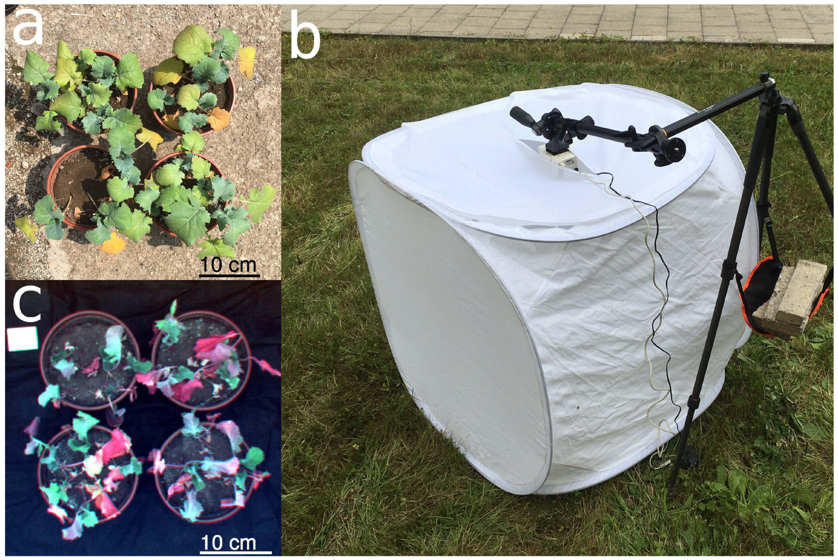
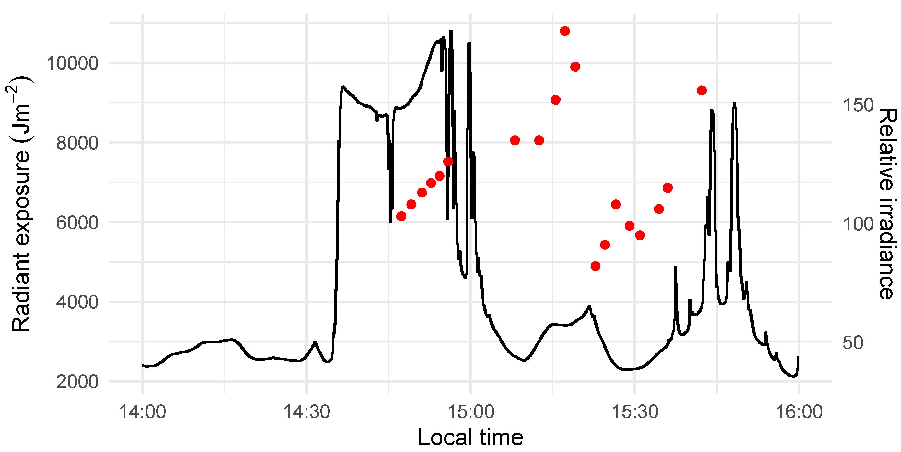
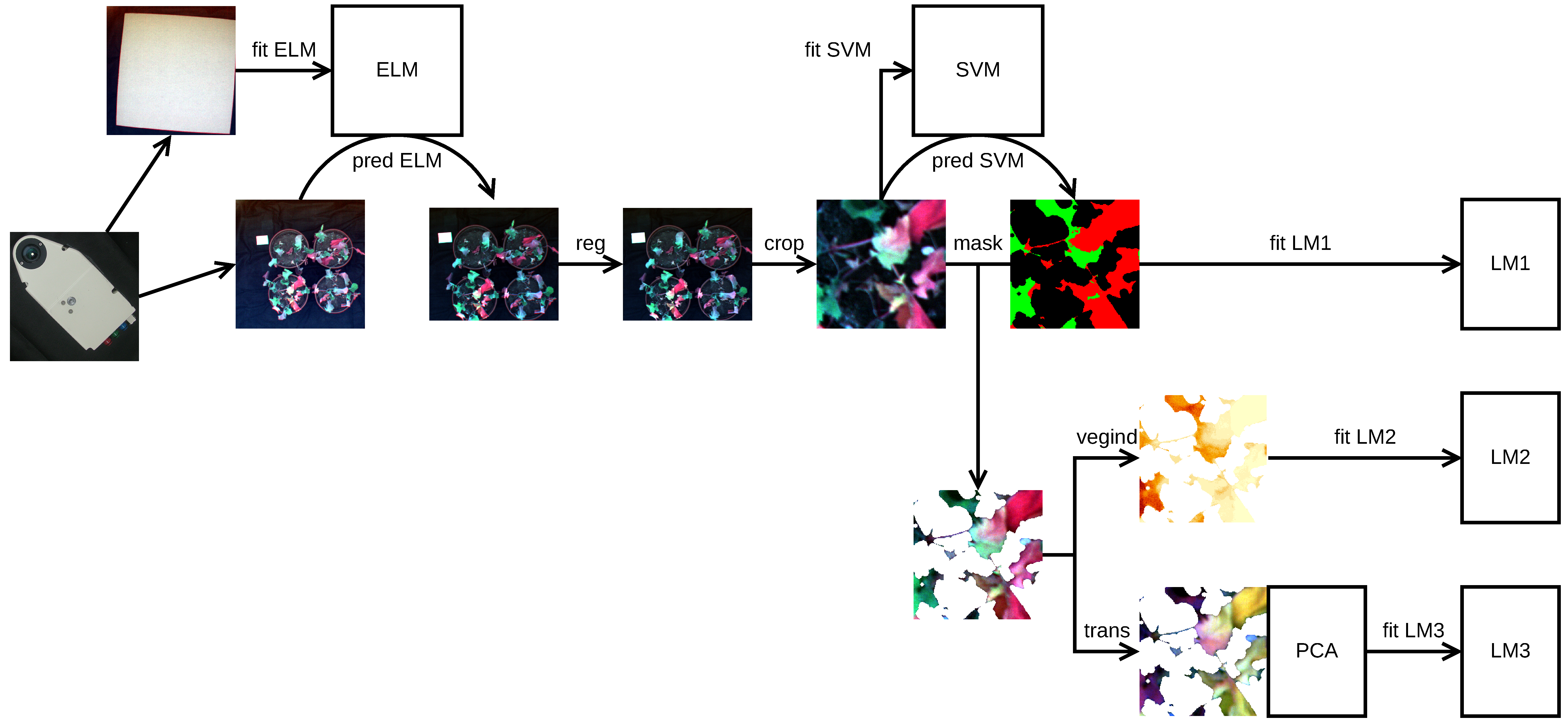
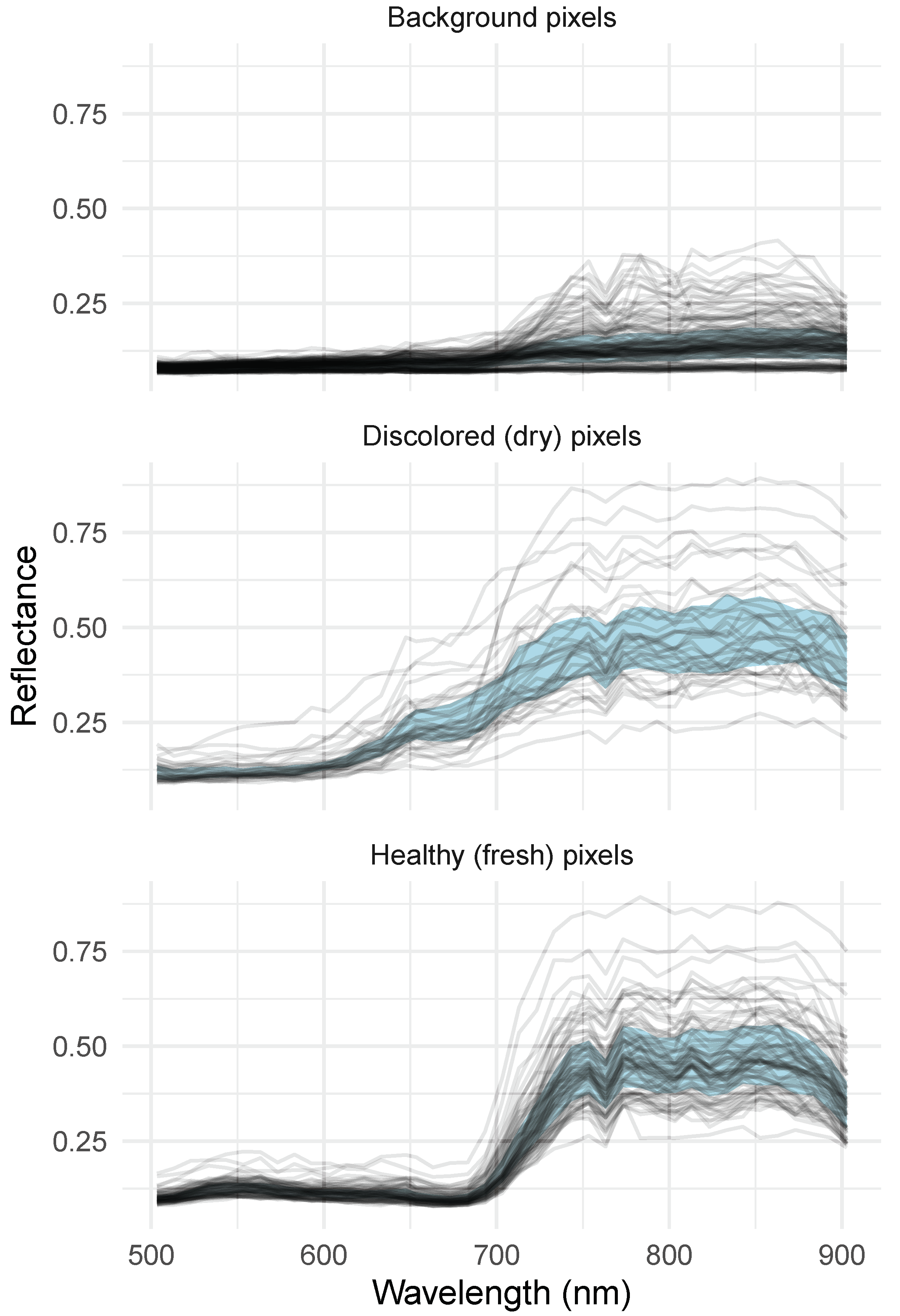
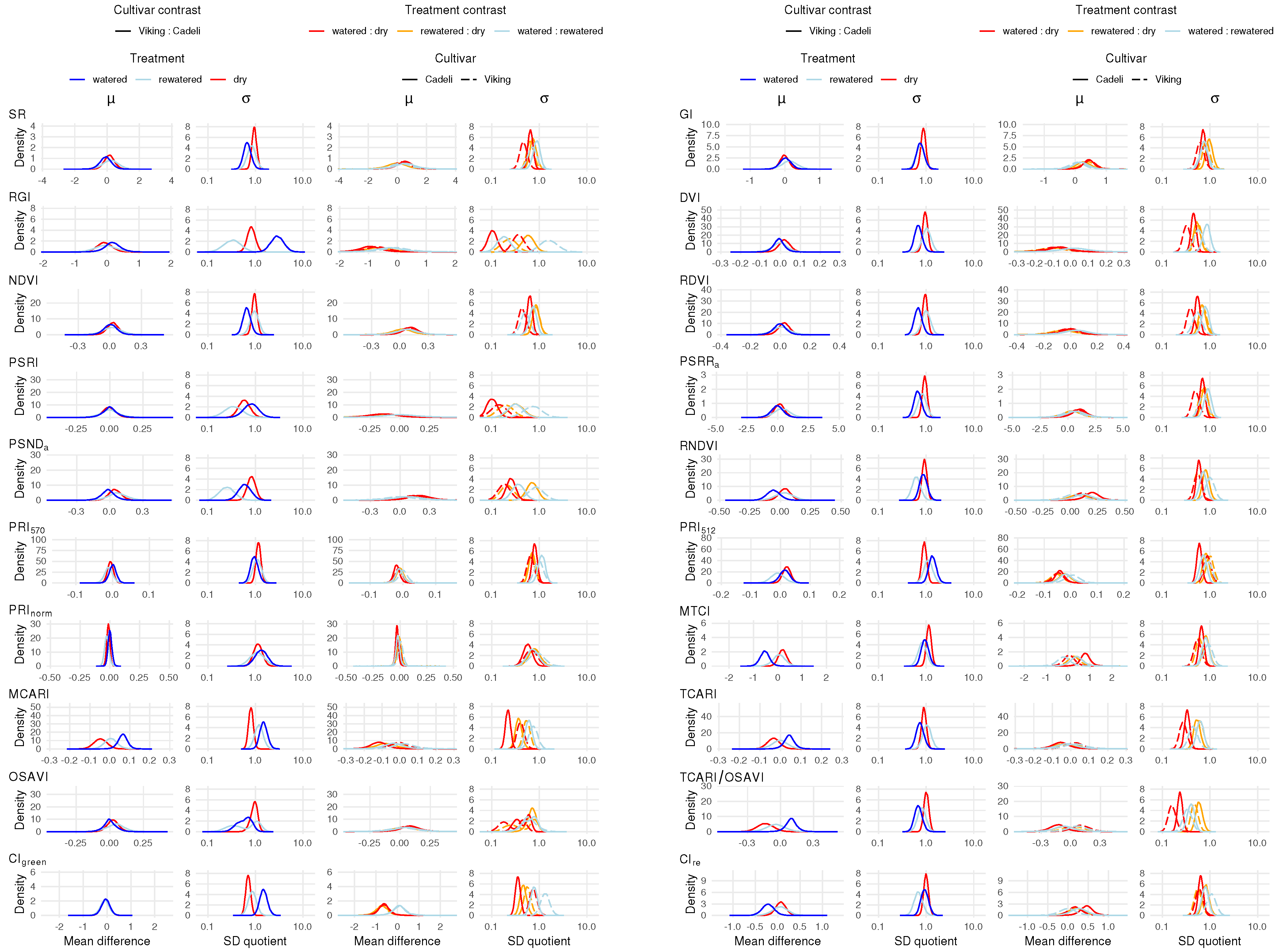
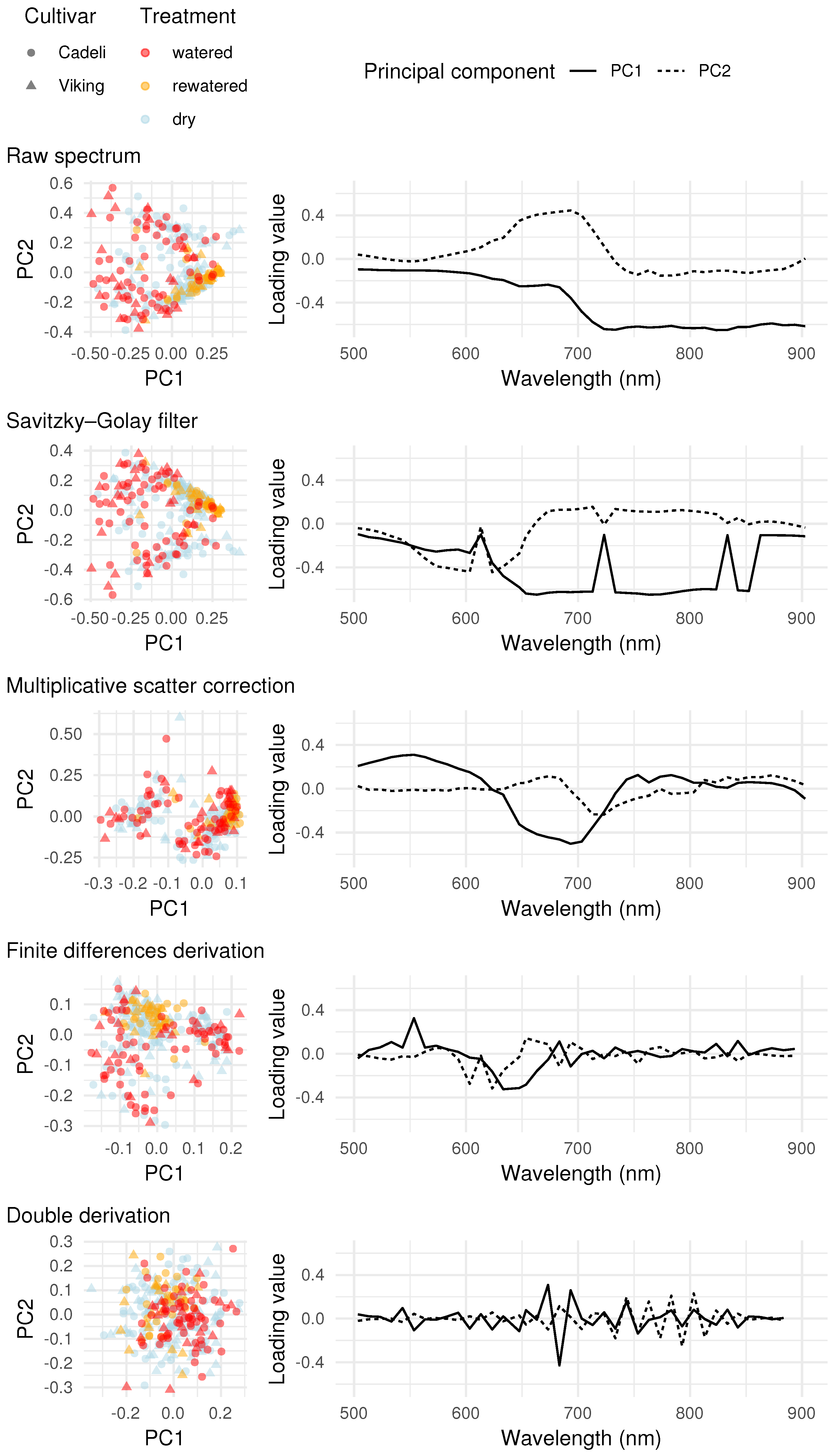
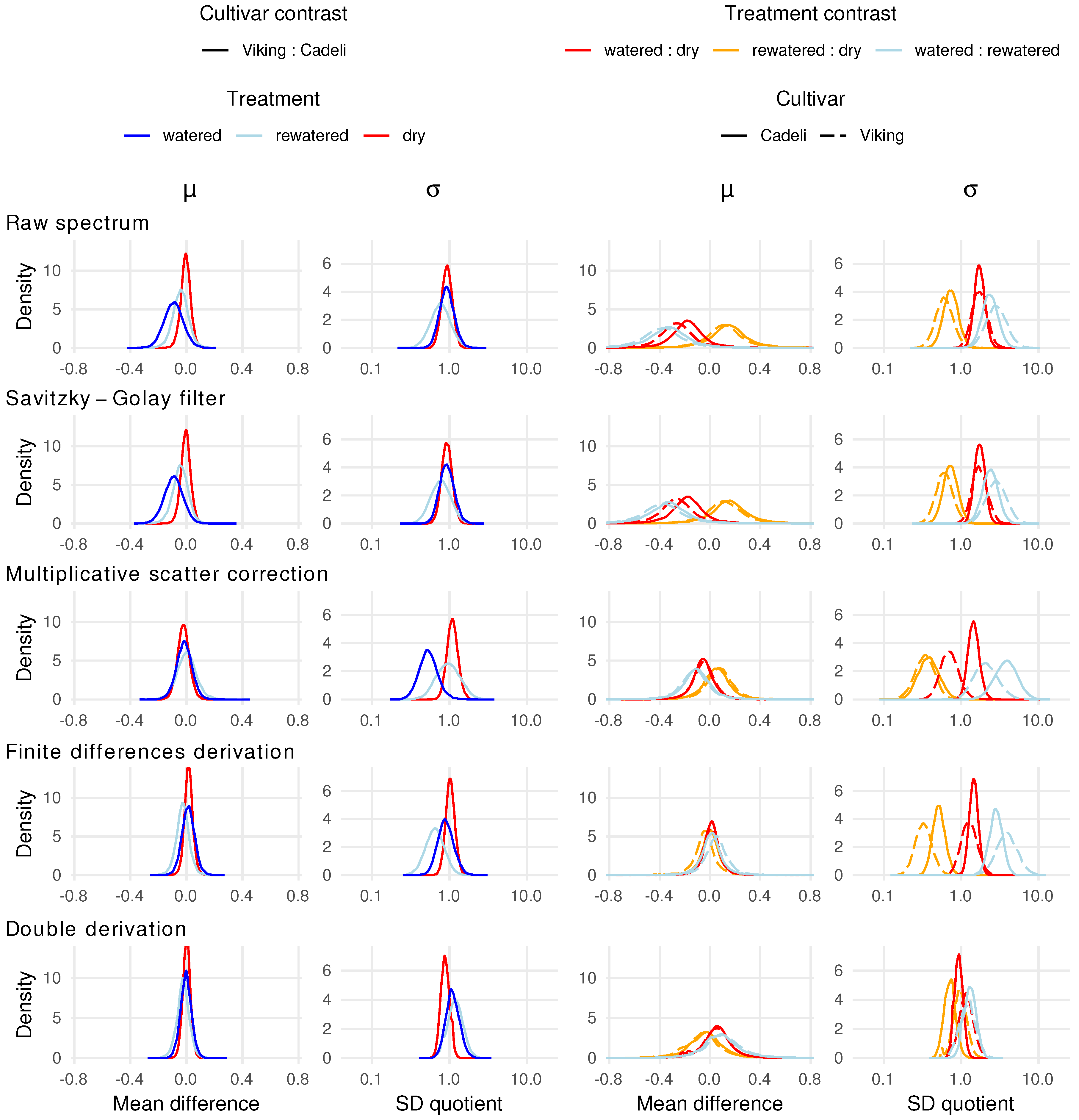
Table 1.
Oilseed rape pot counts used in the experiment according to the experimental treatments. The parenthesised values refer to the counts after excluding a low-quality image.
Table 1.
Oilseed rape pot counts used in the experiment according to the experimental treatments. The parenthesised values refer to the counts after excluding a low-quality image.
| Watering Regime | Cultivar | |
|---|---|---|
| Cadeli | Viking | |
| dry | 6 | 6 |
| rewatered | 3 (2) | 3 (2) |
| watered | 5(0) | 3(0) |
Table 2.
Vegetation indexes used in the study, and their reported sensitivities to biochemical, physiological, and structural plant properties.
Table 2.
Vegetation indexes used in the study, and their reported sensitivities to biochemical, physiological, and structural plant properties.
| Vegetation Index | Formula | Sensitivity | Reference |
|---|---|---|---|
| SR | Chl, fIPAR, LAI | [69] | |
| GI | Chl | [70] | |
| RGI | Chl | [70] | |
| DVI | LWC | [71] | |
| NDVI | Chl, fIPAR, LAI | [69] | |
| RDVI | fAPAR | [72] | |
| PSRI | Chl, Car | [73] | |
| PSSRa | Chl, Car | [74] | |
| PSNDa | Chl, Car | [74] | |
| RNDVI | Chl | [75] | |
| PRI570 | ΔF/Fm’ | [76] | |
| PRI512 | Gs, ᴪ, EPS | [77] | |
| PRInorm | Gs, ᴪ | [78] | |
| MTCI | Chl | [79] | |
| MCARI | Chl | [80] | |
| TCARI | Chl | [81] | |
| OSAVI | LAI | [82] | |
| TCARI/OSAVI | Chl | [81] | |
| CIgreen | Chl | [83] | |
| CIre | Chl | [83] |
Car = carotenoids, Chl = chlorophyll, EPS = violaxanthin:antheraxanthin:zeaxanthin balance, ΔF/Fm’ = fluorescence-based PSII light use efficiency, fAPAR = fractional absorbed PAR, fIPAR = fractional intercepted PAR, Gs = stomatal conductance, LAI = leaf area index, LWC = leaf water content, ᴪ = leaf water potential.
Table 3.
Validation results of the Support Vector Machine (SVM) pixel classification model.
| Observed Classes | Predicted Classes | ||
|---|---|---|---|
| b | d | f | |
| background | 26 | 0 | 1 |
| dry | 0 | 8 | 1 |
| fresh | 0 | 0 | 11 |
Publisher’s Note: MDPI stays neutral with regard to jurisdictional claims in published maps and institutional affiliations. |
© 2020 by the authors. Licensee MDPI, Basel, Switzerland. This article is an open access article distributed under the terms and conditions of the Creative Commons Attribution (CC BY) license (http://creativecommons.org/licenses/by/4.0/).
Share and Cite
MDPI and ACS Style
Żelazny, W.R.; Lukáš, J. Drought Stress Detection in Juvenile Oilseed Rape Using Hyperspectral Imaging with a Focus on Spectra Variability. Remote Sens. 2020, 12, 3462. https://0-doi-org.brum.beds.ac.uk/10.3390/rs12203462
AMA Style
Żelazny WR, Lukáš J. Drought Stress Detection in Juvenile Oilseed Rape Using Hyperspectral Imaging with a Focus on Spectra Variability. Remote Sensing. 2020; 12(20):3462. https://0-doi-org.brum.beds.ac.uk/10.3390/rs12203462
Chicago/Turabian StyleŻelazny, Wiktor R., and Jan Lukáš. 2020. "Drought Stress Detection in Juvenile Oilseed Rape Using Hyperspectral Imaging with a Focus on Spectra Variability" Remote Sensing 12, no. 20: 3462. https://0-doi-org.brum.beds.ac.uk/10.3390/rs12203462
Note that from the first issue of 2016, this journal uses article numbers instead of page numbers. See further details here.