Article

Small-UAV Radar Imaging System Performance with GPS and CDGPS Based Motion Compensation

1
Institute for Electromagnetic Sensing of the Environment (IREA), National Research Council (CNR), 80124 Napoli, Italy
2
Department of Industrial Engineering (DII), University of Naples “Federico II”, via Claudio 21, 80124 Naples, Italy
*
Author to whom correspondence should be addressed.
Remote Sens. 2020, 12(20), 3463; https://0-doi-org.brum.beds.ac.uk/10.3390/rs12203463
Submission received: 16 July 2020 / Revised: 13 October 2020 / Accepted: 19 October 2020 / Published: 21 October 2020
(This article belongs to the Section Engineering Remote Sensing)

Abstract

:
The present manuscript faces the problem of performing high-resolution Unmanned Aerial Vehicle (UAV) radar imaging in sounder modality, i.e., into the vertical plane defined by the along-tack and the nadir directions. Data are collected by means of a light and compact UAV radar prototype; flight trajectory information is provided by two positioning estimation techniques: standalone Global Positioning System (GPS) and Carrier based Differential Global Positioning System (CDGPS). The radar imaging is formulated as a linear inverse scattering problem and a motion compensation (MoCo) procedure, accounting for GPS or CDGPS positioning, is adopted. The implementation of the imaging scheme, which is based on the Truncated Singular Value Decomposition, is made efficient by the Shift and Zoom approach. Two independent flight tests involving different kind of targets are considered to test the imaging strategy. The results show that the CDGPS supports suitable imaging performance in all the considered test cases. On the other hand, satisfactory performance is also possible by using standalone GPS when the meter-level positioning error exhibits small variations during the radar integration time.

Graphical Abstract

1. Introduction

Radar imaging by Unmanned Aerial Vehicle (UAV) platforms [1,2] is worth attention in the remote sensing community as a cost-effective solution to cover wide and/or not easily accessible regions, with high operative flexibility [3]. Indeed, Multicopter-UAVs (M-UAV) have vertical lift capability, allow take-off and landing from very small areas, without the need of long runways or dedicated launch and recovery systems, and, they are able to hover and move in any directions. These peculiar features allow their use at any places and under different flight modes, thus introducing new attractive possibilities in radar remote sensing [4].
UAV based radar imaging can be used in several civil [4] and military applications [5], such as surveillance, security, diagnostics, monitoring in civil engineering, cultural heritage and earth observation, with particular emphasis on natural disasters [6]. At the state of the art, M-UAV radar imaging has been proposed in biomass mapping [7], glaciology [8] and for precision farming [9]. In addition, M-UAVs have been also exploited to perform Synthetic Aperture Radar (SAR), for monitoring small areas and avoiding large platforms. In this context, a first experimentation concerning interferometric P and X band SAR sensors on board a UAV platform has been reported in [10]; moreover, a novel UAV polarimetric SAR system [11] and a multiband drone-borne SAR system [12] have been recently proposed. UAVs have been also exploited in the frame of subsoil exploration by means of Ground Penetrating Radar (GPR) for mine detection [13,14,15,16], soil moisture mapping [17], and detecting subsurface Improvised Explosive Devices (IEDs) [18].
In all of these promising examples, different solutions have been devised to estimate the UAV flight trajectory. For instance, in [7] the ultra-wideband radar PulsON 410 (3.1–5.3 GHz) is used and altitude variations during the flight are corrected by exploiting the reflections from the ground. In [15], a wideband Frequency-Modulated Continuous-Wave (FMCW) GPR, working in the frequency range from 1 GHz to 4 GHz and in a bistatic configuration is proposed; the flight is controlled by manual piloting and a Light Detection and Ranging (LIDAR) is used as the only positioning device for measuring the flight altitude above ground. A standalone Global Positioning System (GPS) is used in [17] for positioning a stepped-frequency continuous-wave (SFCW) radar working in the range from 1 MHz to 6 GHz. Conversely, a sophisticated positioning system is exploited in [14,18] to perform SAR imaging. In [14], a compact pulse radar working in the 3.1 to 5.1 GHz frequency band is considered and a Real Time Kinematic (RTK) system as well as a LIDAR altimeter are used to achieve the cm-level accuracy positioning. In [18], high-resolution 3D SAR imaging is carried out by means of an M-sequence Ultra-Wide-Band (UWB) radar covering a frequency range from 100 MHz to 6 GHz. This radar system is mounted on a UAV, which autonomously flies over a region of interest. The flight is controlled by means of the UAV flight controller, an Inertial Measurement Unit (IMU), a barometer, and a Global Navigation Satellite System (GNSS) receiver. In addition, a laser rangefinder and a dual-band RTK system are exploited to enhance the accuracy of positioning data.
According to the survey just presented, general considerations are:
(i) Accurate UAV positioning data improve the radar imaging performances by avoiding defocusing and localization errors [19];
(ii) Accurate knowledge of the UAV flight trajectory depends strongly on the quality of both the embarked navigation sensors and the deployed ground-based aids [20].
Furthermore, small M-UAVs are constrained by the maximum payload mass and by cost considerations, thus, limiting number and typology of on-board devices.
This work deals with the impact of standalone GPS and Carrier based Differential Global Positioning System (CDGPS) positioning accuracy on small M-UAV radar imaging performed in sounder modality. Therefore, differently from [21], the imaging is faced into a vertical domain, which is a portion of the plane defined by the along-track and the nadir directions. The imaging strategy is similar to the one proposed in [22,23]. It formulates the radar imaging as a linear inverse scattering problem and uses the Truncated Singular Value Decomposition (TSVD) inversion scheme to get a regularized solution. Since the TSVD algorithm requires significant computing resources, especially when increasing the amount of data and the size of the investigated domain (in terms of the probing wavelength), the Shift and Zoom strategy [24] is exploited. The herein adopted imaging strategy benefits of a motion compensation (MoCo) procedure. MoCo exploits GPS or CDGPS positioning information to manage radar measurements in such a way to obtain datasets wherein the waveforms appear as collected at a constant altitude and evenly spaced along a straight line, which defines the along-track direction. It is worth pointing out that, like the approaches proposed in [14,21,23], the adopted imaging strategy can be implemented in such a way to consider the positioning information in the focusing step directly. On the other hand, the MoCo procedure allows a not trivial improvement of the computational effectiveness because it avoids the computation of the scattering operator, and of its SVD, for each portion of dataset to be processed.
In order to evaluate the effect of the UAV positioning accuracy on the imaging capabilities, two experiments were conducted in different weather conditions, i.e., during summer and winter seasons, and by using targets having different geometrical and electromagnetic features. The analysis of the radar imaging performance is carried out in terms of target detection as well as of estimating the relative distance among the targets and their elevation from the ground.
The paper is organized as follows. Section 2 describes the technological instrumentation used to realize the M-UAV based radar imaging prototype, the positioning estimation technologies and the signal processing strategy. Section 3 describes the two measurement campaigns conducted and reports also a qualitative analysis of the imaging results. Then, Section 4 discusses the achieved results. Conclusions end the paper.

2. Materials and Methods

2.1. Measurement Devices

The M-UAV radar prototype described in [22] and shown in Figure 1a is used to collected radar data. A second ground-based GPS receiver (see Figure 1b) is also deployed for the implementation of the CDGPS.
The detailed description of the M-UAV prototype with all mechanical and electronic devices is given in [22]. Here, we briefly summarize the main hardware components:
  • Small M-UAV platform: DJI F550 hexacopter is a mini UAV able to fly at a very low speed (below 1 m/s), ensuring a dense data sampling, and is capable of taking-off and landing from a constrained area;
  • Radar system: PulsON P440 is a compact and short range radar able to transmit ultra-wide band pulses (about 1.7 GHz bandwidth) in the frequency spectrum between the S and C Bands (3.95 GHz carrier frequency) [25];
  • Radar antennas: the radar system has been equipped with two Ramsey LPY26 antennas, which are log-periodic PCB antennas, having a radiation pattern whose aperture angle is of about 80° in the along-track and 110° in the across-track;
  • GPS receivers: two single frequency, single constellation (GPS-only) u-blox LEA-6T devices, one mounted onboard the UAV and the other one used as ground-based station;
  • CPU controller: Linux-based ODROID XU4, which is devoted to manage data acquisition for both radar system and onboard GPS receiver, while assuring the time synchronization between radar and GPS clocks.
The radar module is mounted very close to the flight battery, below the UAV autopilot, see Figure 1a. The distance between the radar antennas and the drone center of mass is about 10 cm. Identical antennas, pointing at nadir direction (down-looking mode) [26] are used to transmit the probing signal and receive the backscattered one. The radar operates in monostatic mode being the distance between the transmitting and receiving antennas negligible in terms of the radar signal wavelength.

2.2. UAV Positioning Techniques

Two standard positioning techniques are considered, such as standalone GPS and CDGPS. One of the two single frequency u-blox LEA-6T devices is installed onboard the drone; while the other one acts as the ground station for CDGPS. The synchronization in time between positioning and radar data is assured by means of the strategies summarized in Figure 2. These strategies have been implemented by means of a dedicated software (written in C language), which exploits the internal CPU clock to tag GPS and radar data during the acquisition stage. Thanks to the common CPU clock reference tag, synchronization between standalone GPS and radar data is performed, while synchronization between CDGPS and radar data is achieved by exploiting GPS time.

2.2.1. Standalone GPS

In general, The UAV positioning estimation system A exploits only the information acquired by the on-board GPS receiver (see Figure 2a). Standalone Global Navigation Satellite System (GNSS) indicates the standard positioning service (see chapter 7 in [27], where basic equations can be found), which processes pseudo-range observables to derive in an epoch-wise fashion to estimate the absolute position of the UAV, e.g., in the World Geodetic System 1984 (WGS 84) reference frame. The attention is here focused on GPS due to the available receivers. The absolute positioning accuracy achievable by the standalone GPS receiver, is defined by the specifications provided by the U.S. Department of Defense [28] Loosely speaking, absolute GPS localization errors are estimated by the product of the User Equivalent Range Error (UERE), which is the effective accuracy of the pseudo-range, and, the Horizontal Dilution of Precision (HDOP) and Vertical Dilution of Precision (VDOP). Representative values of horizontal and vertical positioning errors, in case of satisfactory GPS visibility conditions, are, respectively, 3.5 m and 6.6 m [29] However, when reasonably short time flights are considered, several error sources (i.e., broadcast clock, broadcast ephemeris, group delay, ionospheric delay and tropospheric delay) are strongly correlated both in space and time [27] and may introduce positioning error, which results in a slow varying bias. In addition, the use of a proper processing strategy, such as carrier-smoothing [27], allow a reduction of the measurement noise [30], thus improving the GPS performance.

2.2.2. Carrier Based Differential GPS

An enhanced strategy to reconstruct UAV positioning is based on the use of CDGPS, which is a recognized technique to enhance the positioning performance accuracy of the onboard GPS and it typically exploits at least one motionless GPS receiver working as a reference station (see Figure 2b). Each GPS receiver collects observables, which are a pseudo-range and a carrier-phase measures for any tracked GPS satellite. Carrier-phase measurements show significantly reduced measurement noise (in the order of 1/100 of GPS signal wavelength, i.e., mm scale) with respect to pseudo-range, but ambiguities appear, so carrier-phase ones are biased measurements [27]. If one is able to resolve the ambiguity, very high accurate positioning is enabled. This can be achieved by differential techniques, i.e., CDGPS, where differences between the measurements collected by two relatively close receivers are computed. The CDGPS technique is, indeed, able to filter out the common errors affecting the two receivers, i.e., satellite clock errors, tropospheric and ionospheric errors, thus, achieving an accurate estimate of the relative position between them.
Relative positioning and ambiguity resolution are herein faced in post processing by means of the open-source software RTKlib [31] Specifically, “Post-Processing Kinematic” (PPK) [27] is implemented by using the RTKPOST [20], which processes single-frequency differential observables. Basic equations for the problem at hand can be found in [20] Note that, depending on the working environment, platform dynamics and receiver quality, two different types of CDGPS solutions can be obtained, i.e., fixed or float solutions [32] In the experiments presented in this paper, the position of the UAV with respect to the reference station is estimated with an accuracy ranging from several cm to less than one cm. The better accuracy is achieved when the fixed solution is available, i.e., integer ambiguities are computed [33].

2.3. Imaging Approach

The block diagram of the applied data processing strategy is described in 
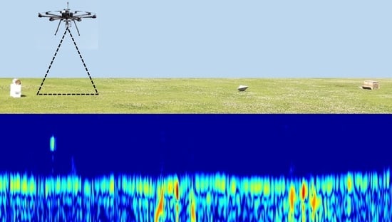
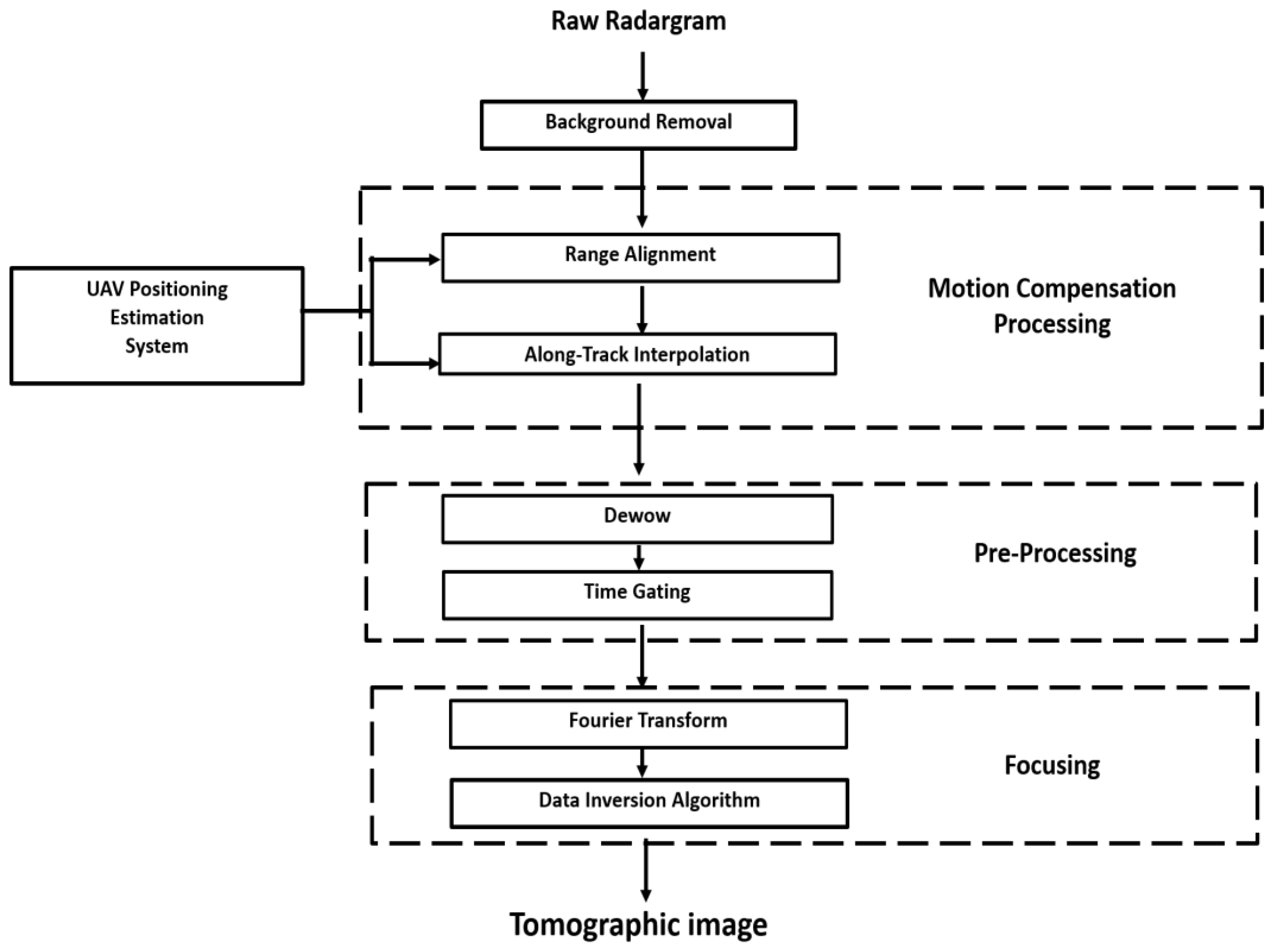
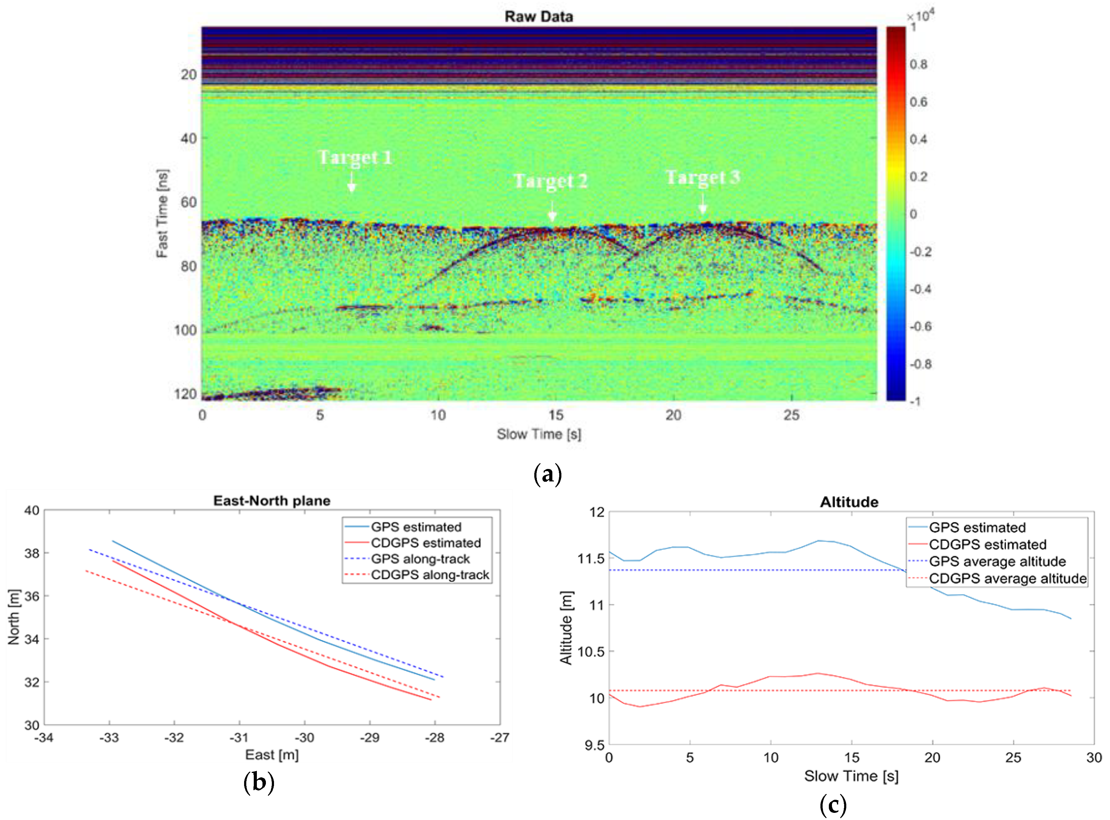
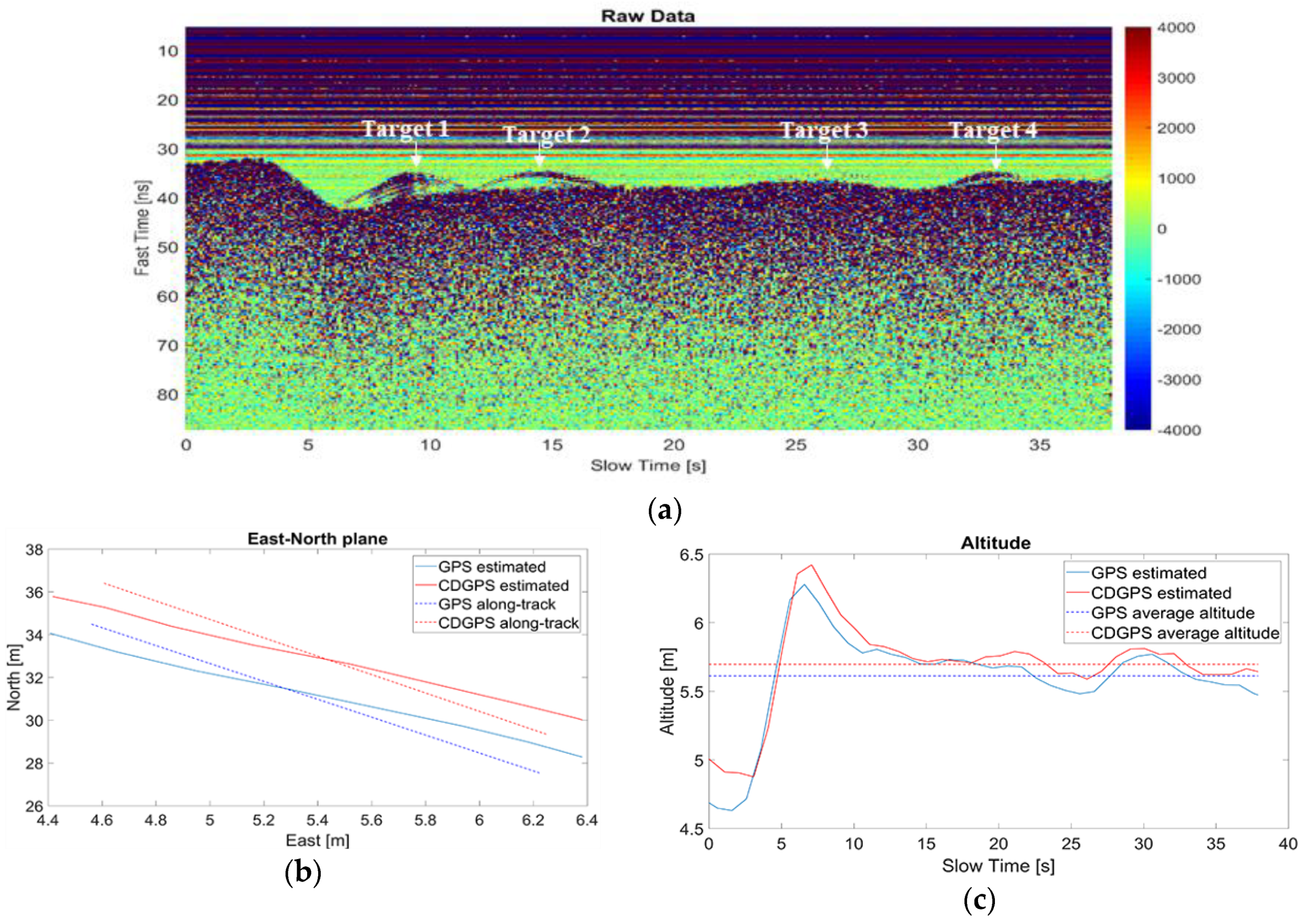
Figure 3. The strategy takes as input the raw radargram, which represents the radar signals collected at each measurement position (during the slow time and along the flight path) versus the fast time. The final output is a focused and easy interpretable image, referred to as tomographic image, which accounts for the reconstruction of the targets into the vertical slice defined by the flight trajectory (along-track direction), which is assumed to be a straight line, and the nadir direction.
Initially, raw data are processed by means of the background removal step [34]. Background removal is a filtering procedure herein adopted for mitigating the undesired signal due to the electromagnetic coupling between transmitting and receiving radar antennas. Since this undesired signal is typically spatial and temporal invariant, the background removal step replaces each single radar trace of the radargram with the difference between the trace and the mean value of all the traces collected along the flight trajectory.
After, the motion compensation (MoCo) stage is performed. The MoCo is a key element of the proposed signal processing strategy and its main steps are depicted in 
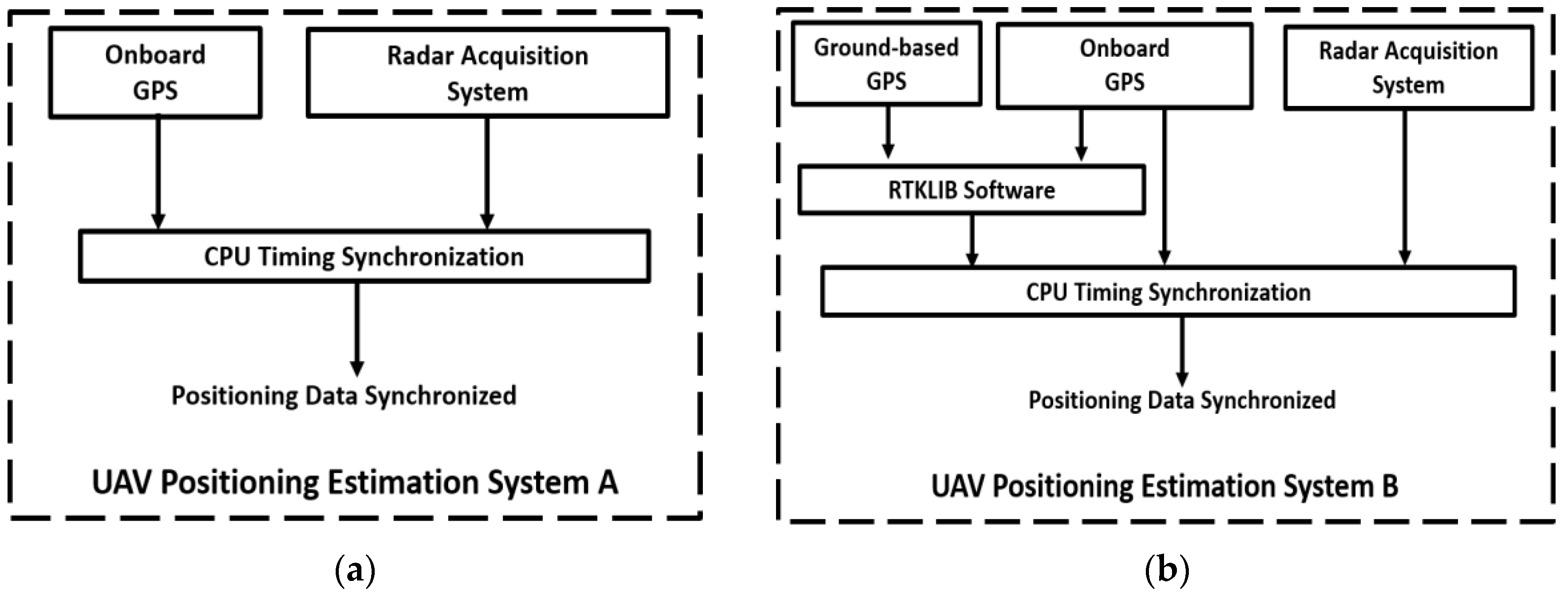
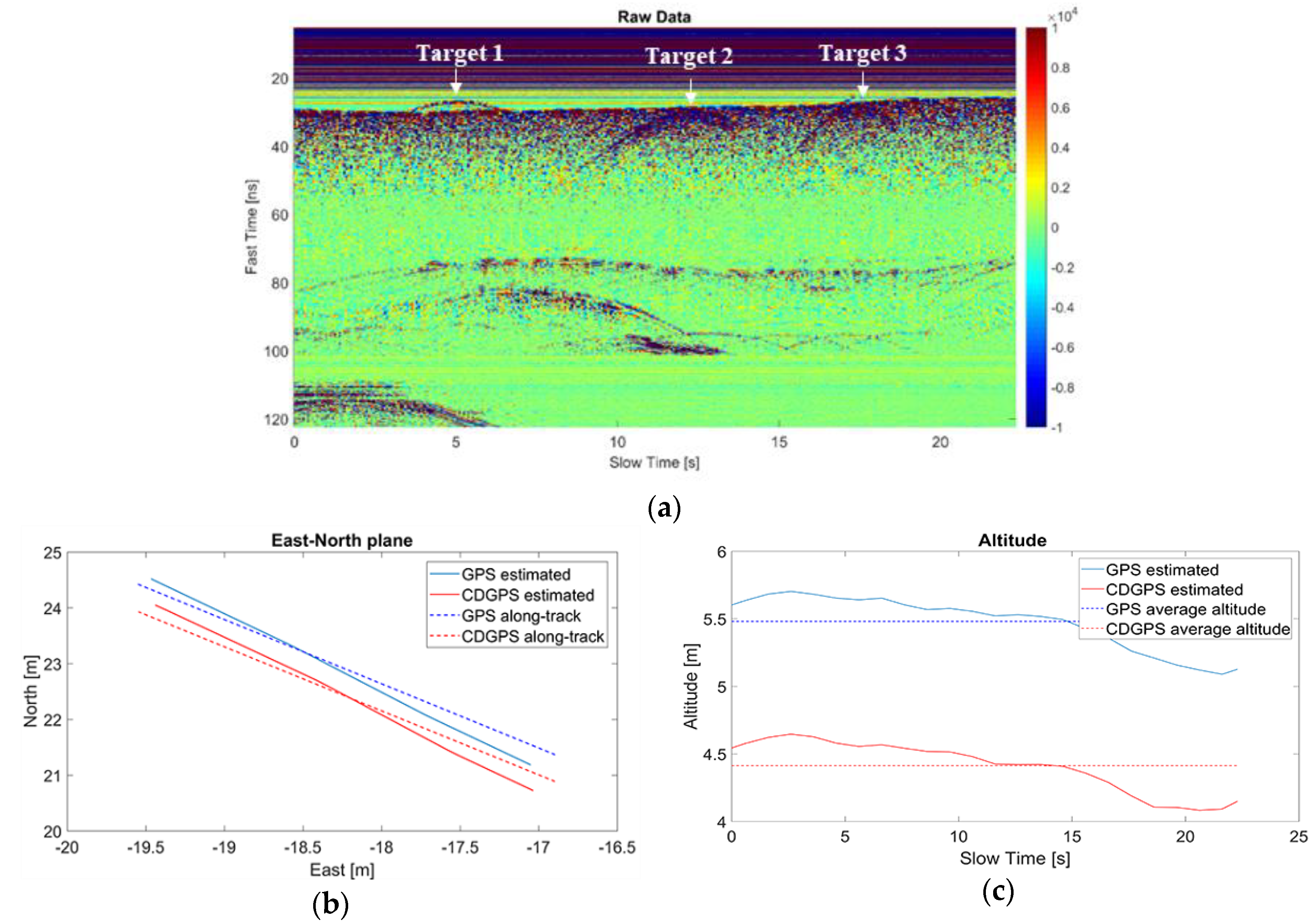
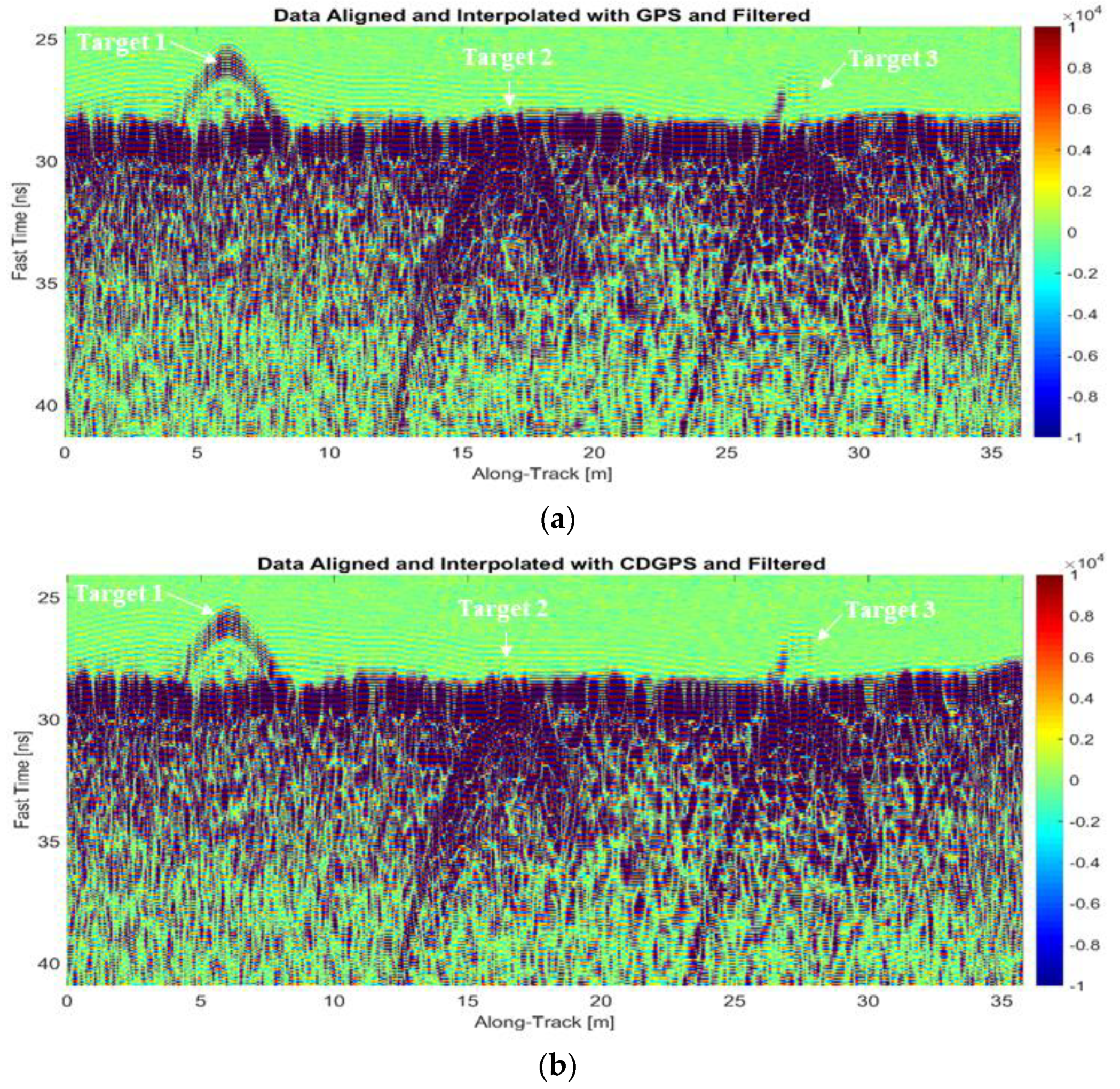
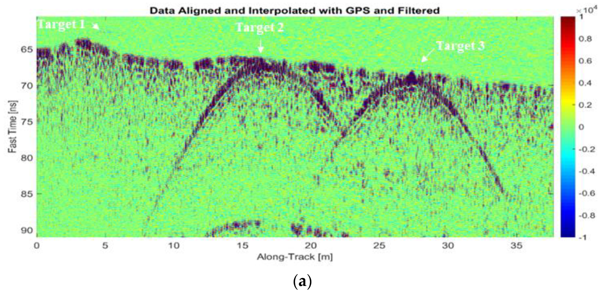
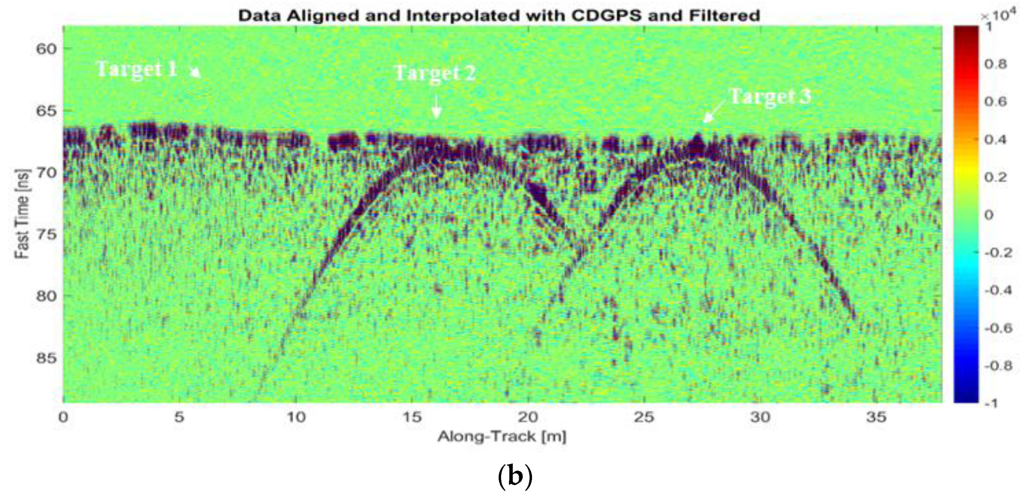
Figure 3. The MoCo takes as input the UAV positions estimated by GPS or CDGPS (defined as “estimated” trajectory), it generates a straight flight trajectory (i.e., the along-track direction) and it modifies the radar signals by means of the range alignment and the along-track interpolation procedures.
The range alignment compensates the altitude variations, occurred during the flight, by realigning each radar signal, along the nadir direction, with respect to a constant flight altitude. This latter is obtained from the UAV altitudes, as estimated by GPS or CDGPS, by an averaging operation, and it is assumed as the altitude of the radar system in the following processing steps.
The along-track interpolation accounts for the deviations occurring in the north–east plane between the estimated flight trajectory and a straight one. In details, a straight trajectory approximating the GPS or CDGPS estimated UAV flight trajectory in the north–east plane is computed by means of a fitting procedure. The straight trajectory in the north–east plane is taken as along-track direction, and is considered as the measurement line in the following processing steps. After the along-track direction is computed, the range aligned radar signals are interpolated and resampled in order to obtain evenly spaced radar data along the along track direction. Attitude variations are not considered in the MoCo. Indeed, the limited distance between the radar antennas and the UAV center of mass and the wide antenna radiation pattern imply that UAV attitude variation has a negligible effect on the data accuracy in terms of two travel time.
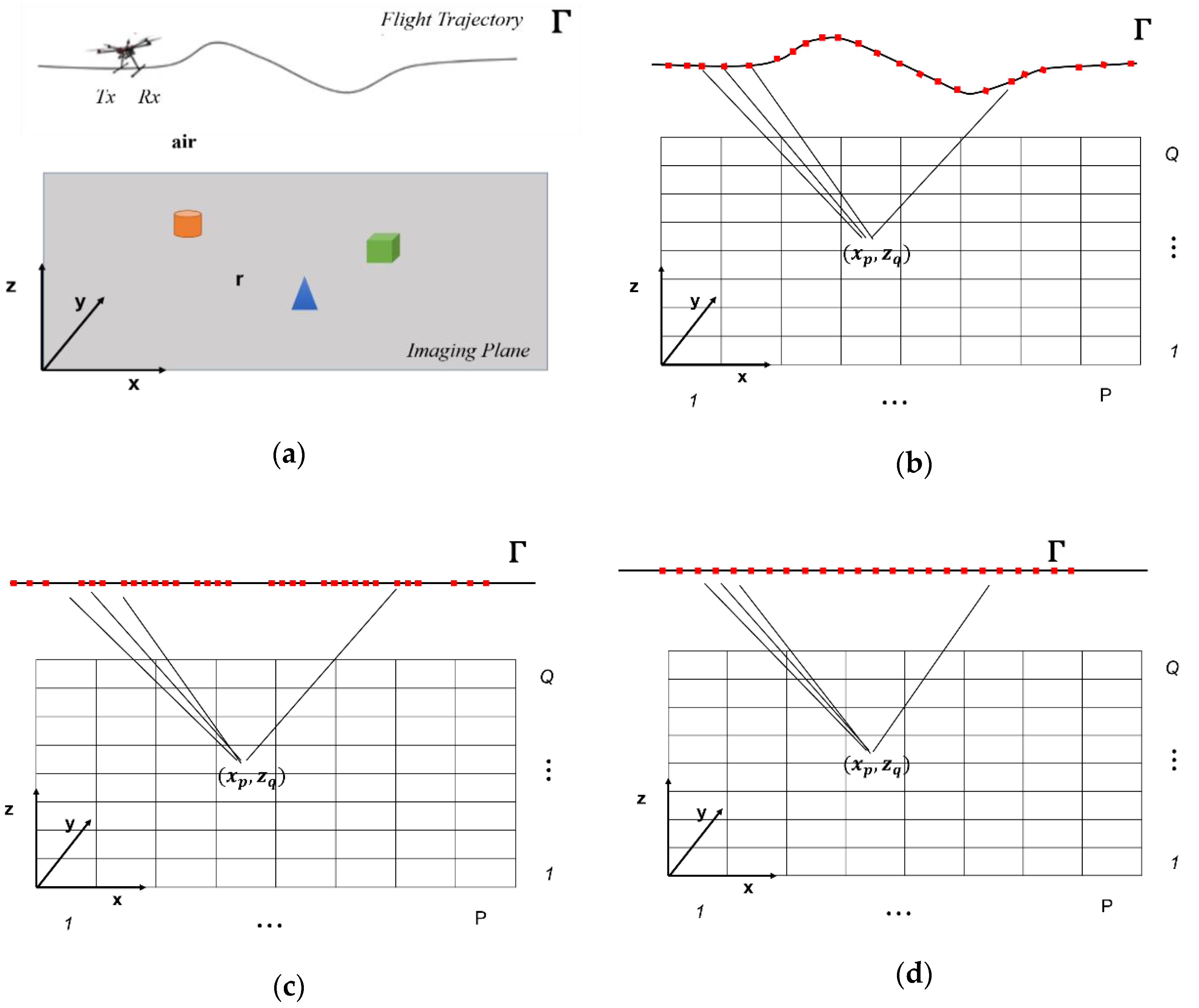
Figure 4a shows a schematic representation of the MoCo. As indicated in Figure 4a,b, originally, the flight trajectory Γ has an arbitrary shape and each measurement points can be indicated by the following unevenly spaced vector: r m = x m x ^ + y m y ^ + z m z ^ . By applying the MoCo, the actual flight trajectory (and accordingly the collected data) is first modified by the range alignment operation as in Figure 4c and, then, by performing the along-track interpolation, the measurements points are evenly spaced, as shown in Figure 4d.
Note that the imaging plane, i.e., the plane wherein the targets are supposed to be located, is the vertical plane defined by the along-track and the nadir directions, from now on indicated as ( x , z ) coordinates, respectively.
After MoCo, the radar data pre-processing step is performed (see Figure 3). At this step, time-domain radar preprocessing procedures as dewow and time gating are carried out. The dewow step aims at mitigating the bias effect induced by internal electronic radar components by removing the average value of each radar trace [34]. The time gating procedure selects the interval (along the fast time) of the radargram, where signals scattered from targets of interest occur. This allows a reduction of environmental clutter and noise effects [35]. Herein, we define a suitable time window around the time where reflection of the air-soil interface occurs.
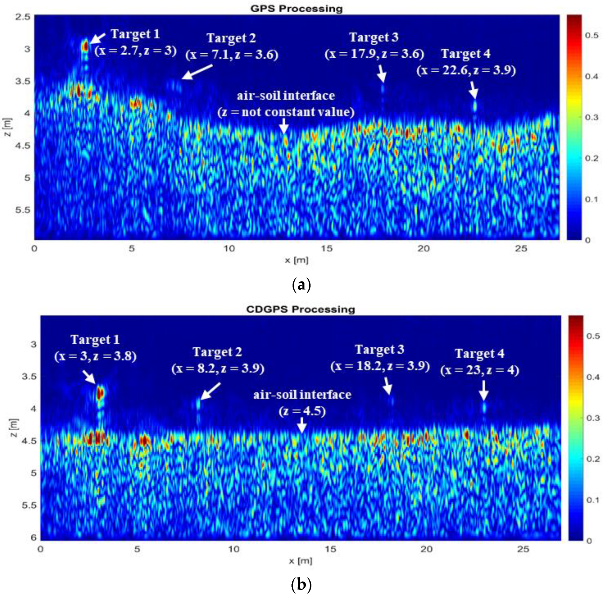
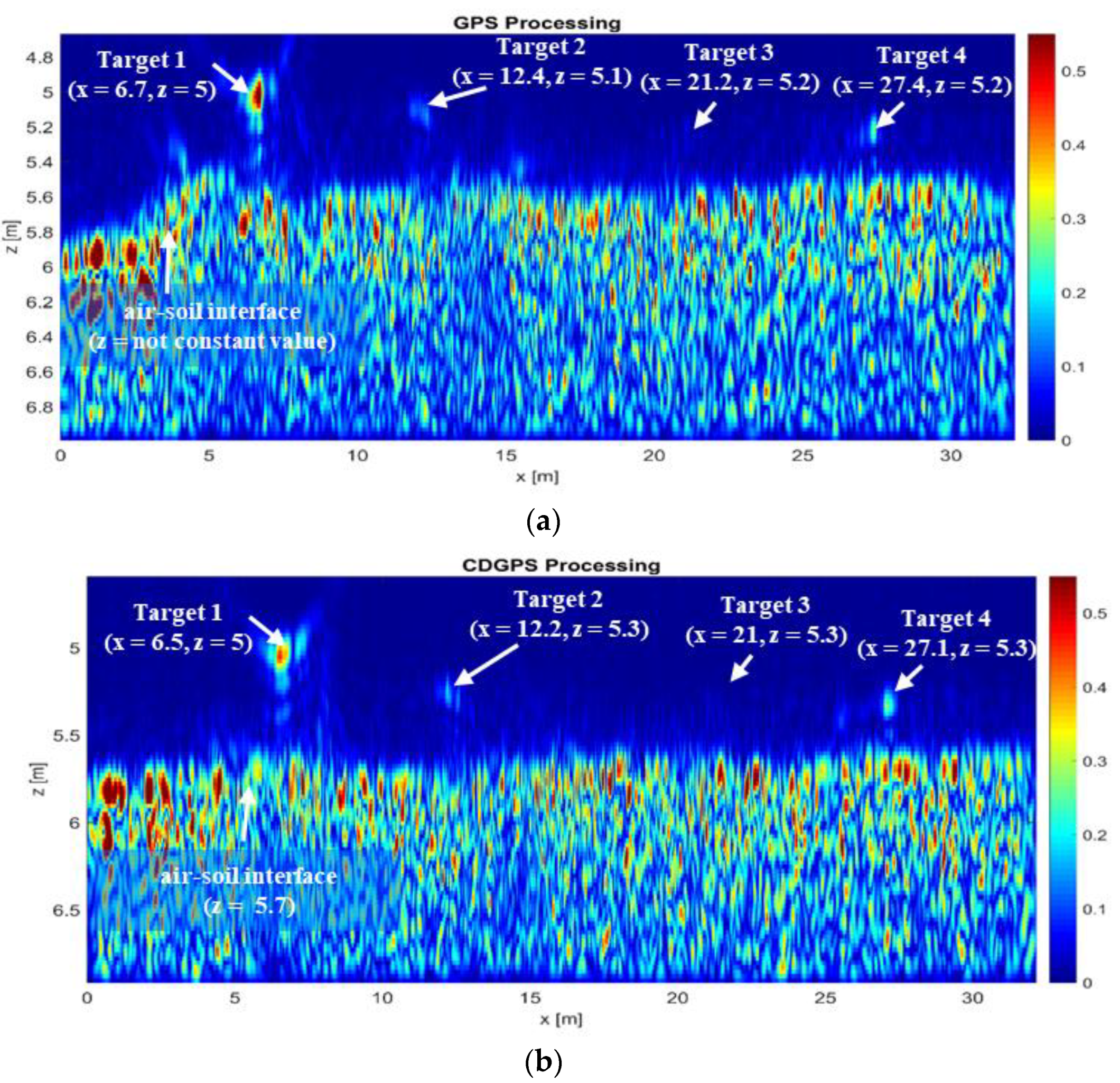
The last processing stage is the focusing. In this stage a focused image of the scene under test, as appearing into the vertical imaging domain, is obtained by solving an inverse scattering problem formulated into the frequency domain. Each trace of the radargram is transformed into the frequency domain by means of the Discrete Fourier Transform (DFT) so to provide the input data to the inversion approach. This latter faces the imaging as an inverse scattering problem by adopting an electromagnetic scattering model based on the following assumptions:
  • The antennas have a broad radiation pattern;
  • The targets are in the far-field region with respect to the radar antennas;
  • A linear model of the scattering phenomenon is assumed, hence the mutual interactions between the targets can be neglected (the Born approximation [36]);
  • The time dependence   e j ω t is assumed, and, for notation simplicity, it is dropped.
Accordingly, at each angular frequency belonging to Ω = [ ω m i n ,   ω m a x ] , which is the angular frequency range of the collected signals, the backscattered signal at each point r m is expressed by the following formula [37]:
E s ( r m , ω ) = S ( ω ) D e j 2 k 0 | r m r |   | r m r | 2 χ ( r ) d r
Equation (1) is a linear integral equation, where S ( ω ) is the spectrum of the transmitted pulse, E s is the measured scattered field, χ ( r ) is the unknown contrast function at a point r = x x ^ + z z ^ in imaging domain D ; k 0 = ω / c 0 is the propagation constant in free space ( c 0 3 · 10 8   [ m / s ] is the speed of light), and, | r m r | is the distance between the measurement point r m and the generic point r in D . The contrast function χ ( r ) accounts for the relative difference between the electromagnetic properties (dielectric permittivity, electrical conductivity) of the targets and the one of the free-space. The spectrum S(ω) is assumed unitary within the frequency range and is omitted for notation simplicity. The kernel of Equation (1) depends on the distance between r m and r ; hence, an accurate knowledge of this relative distance needs to achieve satisfactory imaging capabilities.
The discretized formulation of the imaging problem described in Equation (1) is obtained by exploiting the Method of Moments [38]:
E s = L χ ,
where E s is the K = M × N dimensional data vector, M being the total number of radar scans and N the number of operative pulsations ω n , n = 1 , 2 N . The domain D is discretized by H = P × Q pixels ( x p , z q ) , where p = 1 , 2 P , and q = 1 , 2 Q , χ is the H dimensional unknown vector, and L is the K × H scattering matrix related to the linear operator which maps the space of the unknown vector χ into the space of data (measured scattered field) E s .
The inverse problem defined by Equation (2) is ill posed, thus a regularization scheme needs in order to obtain a stable and robust solution with respect to noise on data [39]:
χ ˜ = n = 1 T 1 σ n < E s , u n > v n ,
where < · , · > denotes the scalar product in the data space, T is the truncation threshold, σ n is the set of singular values of the matrix L ordered in a decreasing way, u n and v n are the sets of the left and right singular vectors. The threshold T K defines the “degree of regularization” of the solution and is chosen as a trade-off between accuracy and resolution requirement from one side (which should push to increase the T value) and solution stability from the other side (which should push to limit the value of T ) [40]. Therefore, the radar image is obtained according to the evaluation of the contrast function in Equation (3).
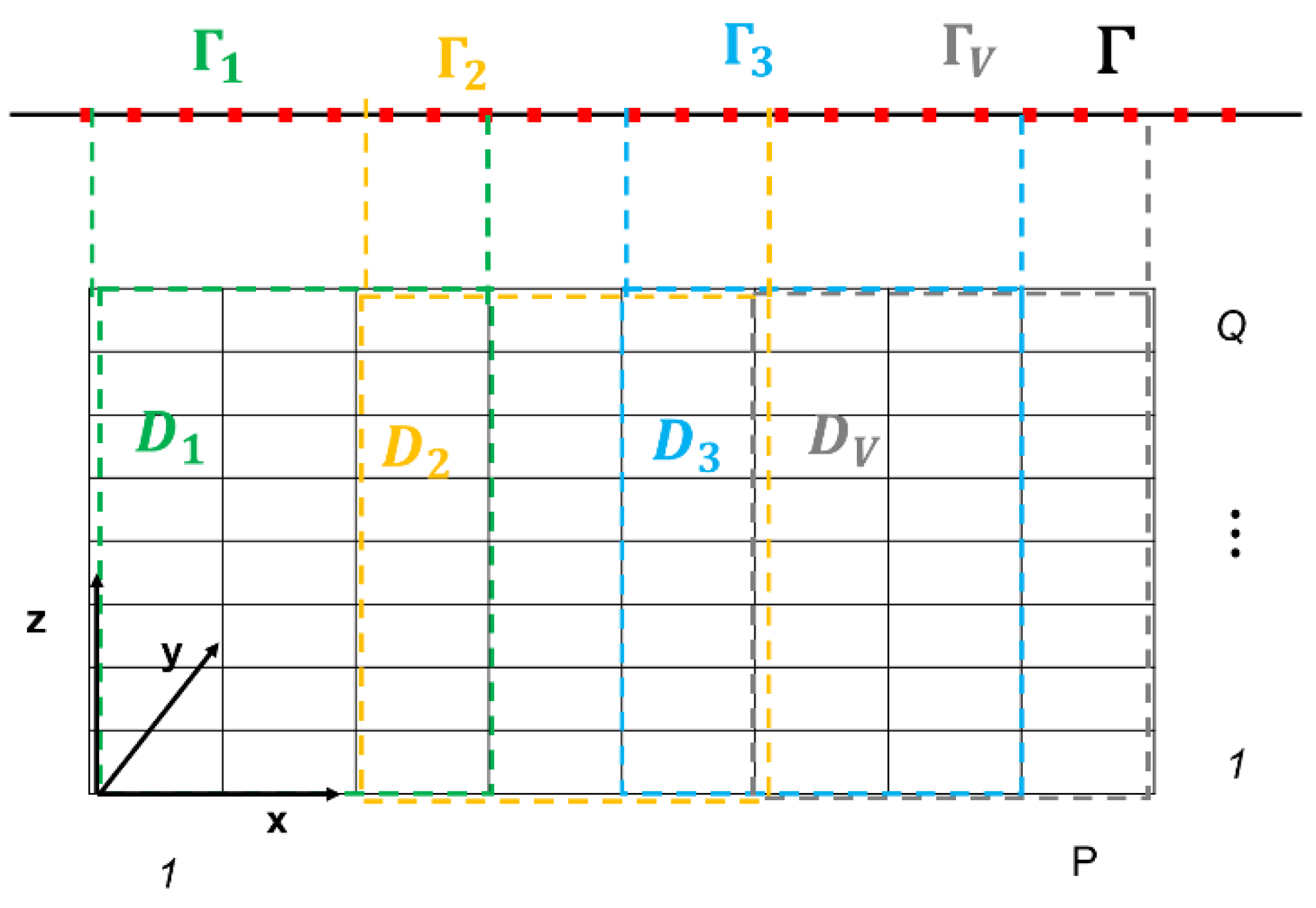
Since the TSVD inversion algorithm is a computational intensive procedure when large (in terms of the probing wavelength) domain are investigated, the Shift and Zoom concept [24] has been implemented in order to speed up the computational time. The Shift and Zoom approach consists in processing data on partially overlapping intervals and combining the images in such a way to get an overall focused image. Specifically, it is schematically represented in Figure 5 and the main steps may be explained as follows:
  • The measurement acquisition line Γ and the survey area D are divided into V partially overlapping subdomains Γ i and D i with i = 1 , 2 , , V ;
  • For each subdomain D i , the tomographic reconstruction χ ˜ i is obtained by the TSVD inversion scheme indicated in Equation (3);
  • The tomographic image of the overall surveyed area D can be obtained by combining the V reconstructions χ ˜ i achieved for each subdomain D i .
A detailed description of the Shift and Zoom implementation is in [27].
Thanks to MoCo, the relative distance between the radar acquisition measurements and the pixel belonging to each subdomain are equivalent for all subdomain. In this way, the SVD calculation of the matrix L have to be evaluated just in a single shot for the first subdomain and the inversion for each subdomain mainly involve matrix times data vector multiplications. By doing so, the computational time for the overall reconstruction process decreases drastically. In fact, the computational cost of the SVD operation for matrix L having size K × H is:
O ( K 2 H )
Conversely, the adoption of the Shift and Zoom approach and the MoCo procedure reduces this cost to:
O ( K α 2 H β )
where α and β are the scaling factors related to reduced size of measurement line Γ i and subdomain D i , respectively. Therefore, an exponential reduction of the computational cost of the TSVD inversion scheme is obtained.

3. Experimental Results

Experimental tests aim at verifying and comparing the radar imaging performance when UAV positioning data are provided by GPS or CDGPS. The imaging capabilities are evaluated in terms of ability to detect targets, to determine their elevation from the ground (i.e., the air-soil interface) and to estimate their relative distance.
The tests have been performed at two different sites: a site for amateur UAV flights testing in Acerra, a small town in suburban area of Naples; a site made available by TopView srl [41] in San Nicola la Strada, a rural area closest to the famous Royal Palace of Caserta, Italy. The experimental tests were carried out during summer and winter seasons, with low or moderate wind conditions, and, by using targets with different geometrical and electromagnetic features.

3.1. First Test Case

The first experimental test was performed on 5 July 2019, during a hot sunny day with weak wind state [21]. Three targets were considered: one cylindrical wood trunk (here referred as target 1) placed at 0.5 m above the ground, whose size are: 0.6 m length and 0.14 m of diameter; two metallic trihedral corner reflectors, having size 0.40   m ×   0.40   m ×   0.57   m   and referred as target 2 and target 3. These latter were used as on-ground targets and target 3 was covered with a cardboard box. The targets were positioned along a straight line, with a relative distance of 10 m (see Figure 6) [21].
The main radar system parameters adopted for data collection are reported in Table 1 [21].
The UAV was manually piloted (in GPS mode) and two flights at different altitudes, herein indicated as Track 1 and Track 2, were carried out. Both tracks were performed on the same scenario by positioning the UAV more or less at the same starting point ( x , y ) .
The first flight had a duration of 22.3 s and covered a 36.5 m long path at the mean flight altitude of about 4.5   m; along this track, data were gathered in 319 not evenly spaced measurement points. Track 2 had a duration of 28.6 s and covered a 33   m long path at an average flight altitude about 10   m; along this track data were gathered in 409 not evenly spaced measurement points.
Figure 7 and Figure 8 depict the raw radargrams (Figure 7a and Figure 8a), the estimated east–north UAV trajectory and the corresponding along-track direction (Figure 7b and Figure 8b), the estimated UAV altitudes and the corresponding average value (Figure 7c and Figure 8c). Specifically, Figure 7b and Figure 8b depict a zoom of the estimated east–north trajectories obtained by means of GPS (blue color) and CDGPS (red color) for both the tracks, respectively. Moreover, these Figures show the corresponding zoom of the along-track directions (dashed blue line—GPS, dashed red line—CDGPS). Similarly, Figure 7c and Figure 8c show, as blue and red solid lines, the estimated altitudes and the corresponding averages (dashed blue and red lines). The dashed lines in Figure 7 and Figure 8 depict the straight line obtained by means of the MoCo.
In Figure 7a, three diffraction hyperbolas corresponding to targets 1, 2, and 3 are clearly visible and their apexes are placed at 5 s, 12.5 s, and 17.5 s along the slow time axis. In Figure 7a, the presence of horizontal constant signals accounts for the antennas coupling, while the signal appearing at fast time values higher than 60 ns are clutter due to lateral objects.
Despite these undesired signals, the UAV radar system is capable of detecting the three targets as well as to recognize that the last encountered corner reflector (target 3) is hidden by a weakly scattering object, as testified by the presence of a small apex above the last hyperbola.
For what concerns Track 2, unfortunately, the hyperbolas related to the target 1 (the wood trunk) is not clearly visible in the raw radargram (see Figure 8a). This effect is due to the smaller intensity of the field backscattered by the trunk being higher flight altitude (the radar transmits the same power whatever the flight altitude is). In Figure 8a, the three hyperbolas related to the three targets have apexes placed at 6 s, 15 s and 21 s along the slow time axis.
In this first test case, GPS and CDGPS provide similar trajectories along the east–north plane, with a slowly varying offset of the order of 1 m (Track 1) or 2 m (Track 2), whereas GPS altitudes are higher than those estimated by CDGPS. Moreover, for Track 1, the GPS and CDGPS UAV altitude profiles differ of a quasi-constant bias; whereas for Track 2 the GPS altitude are affected by a drift (see Figure 7c and Figure 8c, respectively). Given the statistics about the estimated CDGPS uncertainty (based on residuals), reported in Section 4, CDGPS measurements can be assumed as a benchmark for standalone GPS. Thus, the drift of the altitude differences can be interpreted as a vertical error drift for the standalone GPS solution.
Figure 9 and Figure 10 depict the aligned and interpolated radargram after the MoCo and standard time-domain radar preprocessing for Tracks 1 and 2, respectively.
Figure 9 corroborates that in Test 1-Track 1, by using both GPS and CDGPS information, MoCo allows at compensating the altitude variations and, indeed, the air-soil interface appears as an almost flat profile, as it is actually. Conversely, Figure 10 shows that in Test 1-Track 2, while MoCo driven by CDGPS achieves a result similar to Test 1-Track 1, the result based on GPS is worse because the air-soil interface does not have an almost flat profile. This uncompensated effect is due to the drift affecting the estimated GPS altitude (see Figure 8c).
Table 2 and Table 3 list the signal processing parameters adopted to process the radargrams for Track 1 and Track 2 (after MoCo), respectively. The frequency step represents the step used to sample the frequency spectrum of the collected data (ranging from fmin and fmax) and is calculated according to the Nyquist criterion for avoiding aliasing problems [42] in the reconstruction process. The horizontal (i.e., x-axis) size of the overall investigated domain is equal to the extent of the along-track measurement line as defined by the MoCo. Conversely, the vertical (i.e., z-axis) size is such to consider about 1 m up and 2 m below the air-soil interface, whose position is set according to the average altitude value as computed from standalone GPS and CDGPS data. In other words, the zero of the z-axis is in correspondence to the average vertical position of the radar antenna system. Moreover, Table 2 and Table 3 gives the subdomain apertures used to apply the Shift and Zoom procedure, which correspond to 5 m and 7 m for Track 1 and Track 2, respectively. These parameters have been chosen by measuring the target hyperbola extent in the processed radargram and take into account that the hyperbola extent is dictated by the antenna footprint and thus by the flight altitude. This justified why the subdomain aperture considered for the Track 2 is larger than the one used for Track 1.
The tomographic images referred to Test 1-Track 1 and Test 1-Track 2, are depicted in Figure 11 and Figure 12, respectively. These Figures show focused images wherein the metallic corner reflectors are clearly distinguishable, whereas the response of wooden trunk is low due to its lowest reflectivity. Moreover, these figures allow an approximate positioning of the targets.
Figure 11a,b provide an accurate estimation of the altitude of the targets with respect to the air-soil interface; while they give an overestimation of the relative distance among the targets, which is of 1 m in the worst case (i.e., distance between target 2 and target 3 by using GPS data). The air-soil interface appears at z = 5.5 m in Figure 11a and at z = 4.5 m in Figure 11b and this positioning difference is associated to the altitude estimation bias between GPS and CDGPS.
Tomographic reconstructions, depicted in Figure 12a,b, provide an approximate localization of the targets by using both GPS and CDGPS, but standalone GPS data do not allow to correctly reconstruct the air–soil interface profile (it is not flat in Figure 12a).

3.2. Second Test Case

The second test was carried out on the 21 February, 2020, during a cold day with a moderate wind state. In this second case, four targets were placed along a straight line (see Figure 13). Target 1 was a couple of chipboard shelves, having size 0.38   m × 0.60   m , placed at 0.70 m above the ground and with a relative distance of 5 m from the target 2. The target 2 was the same wood trunk adopted in the previous experiment, placed at 0.5 m above the ground and with a distance of 10 m far from target 3. Target 3 was a void inside small box of plasterboard, having size of 0.53   m × 0.53   m × 0.1   m . Finally, as target 4 was used a tuff brick of dimensions 0.27   m × 0.41   m × 0.14   m , placed on ground and far 5 m form target 3. The upper side of target 3 and target 4 are 0.53   m and 0.27   m from the ground, respectively.
Two flights were performed, again with manual UAV piloting in GPS mode. It is worth pointing out that due to the wind effect, Target 3 was repositioned before carrying out the second flight and, in order to assure its stability, which was compromised by foliage presence on the ground, it was located 9 m far from Target 2 and 6 m far from Target 4.
The radar operative parameters adopted for this second test case are reported in Table 4.
The first flight covered 27 m in 41.9 s with an average flight altitude of about 4.2   m; along this track, 420 not evenly points were collected. Track 2 had a duration of 37.9 s and covered 32.20   m with an average altitude of 5.6   m; along this track, 380 unevenly radar scans were collected.
Figure 14 and Figure 15 show the raw radargrams acquired along the two flights and the UAV positions estimated by GPS and CDGPS. Within the east–north plane, positioning differences appear as smoothly varying offsets of several meters (Track 1) or a few meters (Track 2). As concerns the altitude difference, it shows some significant variations during the time interval corresponding to Track 1, while it assumes smaller values in Track 2. As stated above, CDGPS can be assumed as a reference for standalone GPS performance.
The diffraction hyperbolas corresponding to the four targets are clearly visible in Figure 14a and their apexes along the slow time axis are at 9 s, 19 s, 31 s and 37 s. In Figure 15a, the hyperbolas corresponding to Target 1, 2, and 4 can be easily identified at 9 s, 15 s, and 33 s; while the response of Target 3 is less visible. This may be due to less intensity of the backscattered signal caused by the flight altitude, which is higher with respect to the Track 1.
In this second test case, the flight trajectory estimated by GPS and CDGPS have a similar path into the North-East plane, even if there is a bias that is more significant for Track 1 than for Track 2 (see Figure 14b and Figure 15b); while the altitudes exhibit different profiles, even if their average values are quite similar.
The tomographic images referred to Track 1 and Track 2 are depicted in Figure 16 and Figure 17, respectively. These images have been obtained by adopting the signal processing parameters indicated in Table 5 and Table 6, respectively. Respect to the previous test case, here, we want to remark that the Subdomain Apertures have the same size, i.e., 4 m. This parameter has been chosen again by considering the target hyperbola extent in the processed radargrams.
Figure 16b and Figure 17b corroborate that the tomographic images obtained by exploiting CDGPS data are focused images in which the air–soil interface appears flat, as it is actually, and the relative distance among all targets as well as their elevation from the ground are estimated properly. The maximum error is of 0.7 m and regards the estimation of the distance between Target 1 and Targets 2 provided by the tomographic image referred to Track 2.
Focused images allowing an approximated localization of the targets are achieved also by using GPS data even if the imaging capabilities are degraded respect to those obtained by using CDGPS (compare Figure 16a,b as well as Figure 17a,b). Indeed, in Figure 16a and Figure 17a the air–soil interface does not appear flat and the errors on the localization of the targets are larger. These degradations are more visible in Figure 16a than in Figure 17a, i.e., for Track 1.

4. Discussion

The presented results represent a limited number of cases which allow at corroborating some general observations about the reconstruction capabilities of the imaging strategy performed in sounder modality but they do not provide an exhaustive analysis.
A first obvious remark is that targets are detectable if their backscattered signals collected by the radar are distinguishable from clutter and noise. Hence, whatever UAV positioning technology is adopted, the correct number of targets is expected to be identified in the tomographic image even if, depending on their radar cross section, some targets are more clearly visible than other ones.
The second observation is that, as expected, in general the CDGPS positioning data allow better imaging capabilities than standalone GPS data and they made possible to estimate the horizontal distance occurring between targets as well as the target elevation from the ground with a reduced amount of error. This happens even if the achieved CDGPS accuracy was not the same for all the considered examples as it is confirmed by Table 7. This latter reports the percentage of fix/float solution, the number of visible satellites, the average values of Geometric Dilution Of Precision (GDOP), Positional DOP (PDOP), Horizontal DOP (HDOP) Vertical DOP (VDOP), and the mean East, North, and Up Standard Deviations. In other words, even in float mode (estimated positioning uncertainty of several centimeters), CDGPS is shown to effectively support radar imaging.
On the other hand, it is sometime possible that GPS-based motion compensation provides decent radar imaging performance and this happens when space-time correlation of positioning errors is significant. Specifically, the imaging degradation experienced by using GPS occurs when positioning data are affected by drifts, while biases play a less significant role. These results are explained by taking into account the relationship between data and unknowns of the imaging problem, see Equation (1). The kernel of this relationship depends on the knowledge of the relative distance between the UAV radar system and the imaging domain; hence, as more precise is the knowledge of this relative distance as more accurate the imaging results are. In addition, it is worth pointing out that the imaging domain is defined according to the available positioning information. As a consequence, while a constant and unknown bias is detrimental for the absolute localization of the targets, it does not affect the imaging capabilities of the imaging strategy. The bias affecting the generic measurement point r m occurs also in definition of the generic point r of the investigated domain and thus it is erased by computing their distance.
The final remark is about the computational time. As said in the Section 2, the MoCo allows the use of the same scattering operator for the Zoom and Shift implementation of the TSVD based inversion strategy. Therefore, the SVD computation is performed in one single shot and it is used for all the subdomains. The computational time required to obtain the tomographic images are given in Table 8 and are referred to the use of a modern laptop whose main hardware and software characteristics are:
  • Processor: Intel® Core™ i7- 4510U CPU @ 2.00 (GHz)–2.60 (GHz);
  • RAM: 8.00 (GB);
  • Operative System: Windows 10 Pro.
The computational time is in the order of few unit seconds for Test 1-Track 1 and for both tracks of Test 2, i.e., when the average altitudes are in the range of [4.5–5.6] m. Conversely, for Test 1-Track 2, the computational time is about 14 s. This is compliant with the average altitude, which increases up to 10 m. As highlighted before, the higher altitude implies that the Shift and Zoom synthetic aperture adopted for Test 1-Track 2 is larger than those used for the other tracks.
This analysis corroborates that, thanks to the MoCo, the required computational time is compliant with that expected for quasi real-time imaging. In addition, with respect to other classical data inversion strategies, exploiting the positioning information directly in the focusing stage (see [14,18,21]), the MoCo supports the creation of an off line library of scattering operator and their SVD. This feature is useful especially in view of a real-time automatic on board processing for long flight surveys.

5. Conclusions

This manuscript has dealt with UAV radar imaging system and a signal processing strategy for generating high resolution radar images in the plane defined by the nadir range and the along-track directions. The signal processing exploits the MoCo procedure based on standalone GPS or CDGPS positioning data, and faces the imaging as an inverse scattering problem. This latter is solved by means of the TSVD inversion scheme, whose implementation has been speeded up by the Shift and Zoom approach.
To assess the imaging capability and to evaluate the effect of the UAV positioning data on the reconstruction performance, two measurement campaigns have been carried out in different weather conditions (winter and summer) and by using multiple different targets.
The experimental results demonstrate that, in general, inclusion of CDGPS positioning information within the MoCo procedure enables satisfactory imaging results and good target relative localization accuracy, both with fixed and floating solutions. On the other hand, it is sometime possible that standalone GPS-based motion compensation provides suitable radar imaging performance, which happens when space-time correlation of positioning errors is significant. In fact, imaging degradation is associated with the drift of positioning errors during the radar integration time, while biases play a less significant role. This consideration may be important in view of imaging scenarios where CDGPS cannot be used or cannot provide nominal performance levels.
Final comments are dedicated to future developments. First of all, it is necessary to perform an investigation involving a large number of field trials in order to perform an in-depth statistical analysis for quantitatively assessing the impact of the positioning techniques on the imaging system capabilities; in this frame, we will exploit merit figures, such as the achievable resolutions and imaging quality parameters as peak contrast and entropy. Then, an imaging sensitivity comparison analysis between the current MoCo imaging approach and 3D UAV positioning integration in the focusing stage will be conducted. Furthermore, an advanced autonomous flight mode with the possibility to plan the UAV flight on a predesigned grid will be accounted for as well as the use of low frequency radar systems allowing underground penetration capabilities. In this frame, imaging procedures devoted to exploit data gathered along multiple lines will be considered in order to obtain a 3D tomographic reconstruction of the investigated scene. In addition, imaging strategies able to account for the different electromagnetic velocity in air and soil will be considered in case of underground penetration.

Author Contributions

Conceptualization, C.N., I.C., G.F., and F.S.; methodology, C.N., I.C., F.S., and G.F.; software and validation, C.N., I.C., G.E., and G.F.; formal analysis, C.N., I.C., F.S.; investigation, C.N., I.C., G.E., and G.F.; data curation, C.N., I.C., G.E., and G.F.; writing—original draft preparation, C.N., I.C., G.E., A.R., and G.F.; supervision, I.C.; project administration, I.C. and F.S.; funding acquisition, I.C. and F.S. All authors have read and agreed to the published version of the manuscript.

Funding

This research was funded by CAMPANIA FESR Operational Program 2014–2020, under the VESTA project “Valorizzazione E Salvaguardia del paTrimonio culturAle attraverso l’utilizzo di tecnologie innovative” (Enhancement and Preservation of the Cultural Heritage through the use of innovative technologies VESTA), grant number CUP B83D18000320007.

Acknowledgments

The authors would like to thank TopView srl, which made available its UAV test site, thus, allowing to perform the second measurement campaign.

Conflicts of Interest

The authors declare no conflict of interest.

References

  1. Everaerts, J. The Use of Unmanned Aerial Vehicles (UAVs) for Remote Sensing and Mapping. Int. Arch. Photogramm. Remote Sens. Spat. Inf. Sci. 2008, 37, 1187–1192. [Google Scholar]
  2. Quan, Q. Introduction to Multicopter Design and Control; Springer: Singapore, 2017. [Google Scholar]
  3. Colomina, I.; Molina, P. Unmanned aerial systems for photogrammetry and remote sensing: A review. ISPRS J. Photogramm. Remote Sens. 2014, 92, 79–97. [Google Scholar] [CrossRef] [Green Version]
  4. Yao, H.; Qin, R.; Chen, X. Unmanned Aerial Vehicle for Remote Sensing Applications—A Review. Remote Sens. 2019, 11, 1443. [Google Scholar] [CrossRef] [Green Version]
  5. Van Der Graaf, M.W.; Otten, M.P.G.; Huizing, A.G.; Tan, R.G.; Cuenca, M.C.; Ruizenaar, M.G.A. AMBER: An X-band FMCW digital beam forming synthetic aperture radar for a tactical UAV. In Proceedings of the 2013 IEEE International Symposium on Phased Array Systems and Technology, Waltham, MA, USA, 15–18 October 2013; pp. 165–170. [Google Scholar]
  6. Massonnet, D.; Souyris, J.C. Imaging with Synthetic Aperture Radar; EPFL Press: Lausanne, Switzerland, 2008. [Google Scholar]
  7. Li, C.J.; Ling, H. High-resolution, downward-looking radar imaging using a small consumer drone. In Proceedings of the 2016 IEEE International Symposium on Antennas and Propagation (APSURSI), Fajardo, Puerto Rico, 26 June–1 July 2016; pp. 2037–2038. [Google Scholar]
  8. Bhardwaj, A.; Sam, L.; Akanksha, L.; Martín-Torres, F.J.; Kumar, R. UAVs as remote sensing platform in glaciology: Present applications and future prospects. Remote Sens. Environ. 2016, 175, 196–204. [Google Scholar] [CrossRef]
  9. Cunliffe, A.M.; Brazier, R.E.; Anderson, K. Ultra-fine grain landscape-scale quantification of dryland vegetation structure with drone-acquired structure-from-motion photogrammetry. Remote Sens. Environ. 2016, 183, 129–143. [Google Scholar] [CrossRef] [Green Version]
  10. Remy, M.A.; De Macedo, K.A.C.; Moreira, J.R. The first UAV-based P- and X-band interferometric SAR system. In Proceedings of the 2012 IEEE International Geoscience and Remote Sensing Symposium, Munich, Germany, 22–27 July 2012; pp. 5041–5044. [Google Scholar]
  11. Lort, M.; Aguasca, A.; López-Martínez, C.; Marin, T.M. Initial Evaluation of SAR Capabilities in UAV Multicopter Platforms. IEEE J. Sel. Top. Appl. Earth Obs. Remote Sens. 2017, 11, 127–140. [Google Scholar] [CrossRef] [Green Version]
  12. Luebeck, D.; Wimmer, C.; Moreira, L.F.; Alcântara, M.; Oré, G.; Góes, J.A.; Oliveira, L.P.; Mederos, B.J.T.; Bins, L.S.; Gabrielli, L.H.; et al. Drone-Borne Differential SAR Interferometry. Remote Sens. 2020, 12, 778. [Google Scholar] [CrossRef] [Green Version]
  13. Amiri, A.; Tong, K.; Chetty, K. Feasibility study of multi-frequency Ground Penetrating Radar for rotary UAV platforms. In Proceedings of the IET International Conference on Radar Systems (Radar 2012), Glasgow, UK, 22–25 October 2012; p. 92. [Google Scholar]
  14. Fernandez, M.G.; Lopez, Y.A.; Arboleya-Arboleya, A.; Valdes, B.G.; Vaqueiro, Y.R.; Andres, F.L.-H.; Garcia, A.P. Synthetic Aperture Radar Imaging System for Landmine Detection Using a Ground Penetrating Radar on Board a Unmanned Aerial Vehicle. IEEE Access 2018, 6, 45100–45112. [Google Scholar] [CrossRef]
  15. Burr, R.; Schartel, M.; Schmidt, P.; Mayer, W.; Walter, T.; Waldschmidt, C. Design and Implementation of a FMCW GPR for UAV-based Mine Detection. In Proceedings of the 2018 IEEE MTT-S International Conference on Microwaves for Intelligent Mobility (ICMIM), Munich, Germany, 15–17 April 2018; pp. 1–4. [Google Scholar]
  16. Gonzalez-Diaz, M.; Garcia-Fernandez, M.; Lopez, Y.A.; Las-Heras, F. Improvement of GPR SAR-Based Techniques for Accurate Detection and Imaging of Buried Objects. IEEE Trans. Instrum. Meas. 2020, 69, 3126–3138. [Google Scholar] [CrossRef] [Green Version]
  17. Wu, K.; Rodriguez, G.A.; Zajc, M.; Jacquemin, E.; Clément, M.; De Coster, A.; Lambot, S. A new drone-borne GPR for soil moisture mapping. Remote Sens. Environ. 2019, 235, 111456. [Google Scholar] [CrossRef]
  18. García-Fernández, M.; López, Y.Á.; Andrés, F.L.-H. Autonomous Airborne 3D SAR Imaging System for Subsurface Sensing: UWB-GPR on Board a UAV for Landmine and IED Detection. Remote Sens. 2019, 11, 2357. [Google Scholar] [CrossRef] [Green Version]
  19. Soumekh, M. Wavefront-Based Synthetic Aperture Radar Signal Processing; Wiley: New York, NY, USA, 1999; Volume 7. [Google Scholar]
  20. Teunissen, P.; Montenbruck, O. (Eds.) Springer Handbook of Global Navigation Satellite Systems; Springer: Cham, Switzerland, 2017. [Google Scholar]
  21. Catapano, I.; Gennarelli, G.; Ludeno, G.; Noviello, C.; Esposito, G.; Renga, A.; Fasano, G.; Soldovieri, F. Small Multicopter-UAV-Based Radar Imaging: Performance Assessment for a Single Flight Track. Remote Sens. 2020, 12, 774. [Google Scholar] [CrossRef] [Green Version]
  22. Ludeno, G.; Catapano, I.; Renga, A.; Vetrella, A.R.; Fasano, G.; Soldovieri, F. Assessment of a micro-UAV system for microwave tomography radar imaging. Remote Sens. Environ. 2018, 212, 90–102. [Google Scholar] [CrossRef]
  23. Gennarelli, G.; Catapano, I.; Ludeno, G.; Noviello, C.; Papa, C.; Pica, G.; Soldovieri, F.; Alberti, G. A low frequency airborne GPR system for wide area geophysical surveys: The case study of Morocco Desert. Remote Sens. Environ. 2019, 233, 111409. [Google Scholar] [CrossRef]
  24. Persico, R.; Ludeno, G.; Soldovieri, F.; De Coster, A.; Lambot, S. Two-Dimensional Linear Inversion of GPR Data with a Shifting Zoom along the Observation Line. Remote Sens. 2017, 9, 980. [Google Scholar] [CrossRef] [Green Version]
  25. Available online: https://fccid.io/NUF-P440-A/User-Manual/User-Manual-2878444/ (accessed on 20 October 2020).
  26. Richards, M.A. Fundamentals of Radar Signal Processing; Tata McGraw-Hill Education: New York, NY, USA, 2005. [Google Scholar]
  27. Kaplan, E.; Hegarty, C.J. Understanding GPS–Principles and Applications, 2nd ed.; Artech House: Boston, MA, USA; London, UK, 2006. [Google Scholar]
  28. Standard, GSP. Retrieved on July 14, 2008, 2009. ed, 7, 2012.
  29. Milbert, D. Dilution Of Precision Revisited. Navigation 2008, 55, 67–81. [Google Scholar] [CrossRef]
  30. Farrell, J.A. Aided Navigation: GPS with High Rate Sensors; Mc Graw. Hill: New York, NY, USA, 2008. [Google Scholar]
  31. Available online: http://www.rtklib.com/rtklib_document.htm (accessed on 20 October 2020).
  32. Renga, A.; Fasano, G.; Accardo, D.; Grassi, M.; Tancredi, U.; Rufino, G.; Simonetti, A. Navigation Facility for High Accuracy Offline Trajectory and Attitude Estimation in Airborne Applications. Int. J. Navig. Obs. 2013, 2013, 1–13. [Google Scholar] [CrossRef] [Green Version]
  33. Persico, R. Introduction to Ground Penetrating Radar: Inverse Scattering and Data Processing; John Wiley & Sons: Hoboken, NJ, USA, 2014. [Google Scholar]
  34. Catapano, I.; Gennarelli, G.; Ludeno, G.; Soldovieri, F.; Persico, R. Ground-Penetrating Radar: Operation Principle and Data Processing. In Wiley Encyclopedia of Electrical and Electronics Engineering; Wiley: Hoboken, NJ, USA, 2019; pp. 1–23. [Google Scholar]
  35. Daniels, D.J. Ground Penetrating Radar. In Encyclopedia of RF and Microwave Engineering; Wiley: Hoboken, NJ, USA, 2005. [Google Scholar]
  36. Chew, W.C. Waves and Fields in Inhomogenous Media; IEEE Press: Piscataway, NJ, USA, 1999. [Google Scholar]
  37. Balanis, C.A. Advanced Engineering Electromagnetics; John Wiley & Sons: Hoboken, NJ, USA, 1999. [Google Scholar]
  38. Harrington, R.F. Field Computation by Moment Methods; Wiley-IEEE Press: Hoboken, NJ, USA, 1993. [Google Scholar]
  39. Solimene, R.; Catapano, I.; Gennarelli, G.; Cuccaro, A.; Dell’Aversano, A.; Soldovieri, F. SAR Imaging Algorithms and Some Unconventional Applications: A unified mathematical overview. IEEE Signal Process. Mag. 2014, 31, 90–98. [Google Scholar] [CrossRef]
  40. Bertero, M.; Boccacci, P. Introduction to Inverse Problems in Imaging; CRC Press: Boca Raton, FL, USA, 1998. [Google Scholar]
  41. Available online: https://topview.it/en/ (accessed on 20 October 2020).
  42. Proakis, J.G. Digital Signal Processing: Principles Algorithms and Applications; Pearson Education: Bangalore, India, 2001. [Google Scholar]
Figure 1. Multicopter-UAVs (M-UAV) radar imaging system: (left) M-UAV hexacopter with onboard equipment [21]; (right) ground-based Global Positioning System (GPS) station [21].
Remotesensing 12 03463 g001
Figure 2. Positioning and radar data synchronization strategy (a) Standalone GPS; (b) Carrier based Differential Global Positioning System (CDGPS).
Remotesensing 12 03463 g002
Figure 3. Signal Processing Strategy.
Remotesensing 12 03463 g003
Figure 4. The Unmanned Aerial Vehicle (UAV)-borne radar imaging system, (a) actual imaging scenario; (b) starting schematic configuration; (c) schematic configuration after range alignment; (d) schematic configuration after along-track interpolation.
Remotesensing 12 03463 g004
Figure 5. Shift and Zoom Algorithm description.
Remotesensing 12 03463 g005
Figure 6. First test case: radar imaging scenario.
Remotesensing 12 03463 g006
Figure 7. Test 1-Track 1: (a) raw data; (b) east–north UAV positions estimated by GPS (solid blue line) and CDGPS (solid red line), along-track direction defined by GPS (dashed blue line) and CDGPS (dashed red line); (c) UAV Altitude estimated by GPS (solid blue line) and CDGPS (solid red line), average altitude defined by GPS (dashed blue line) and CDGPS (dashed red line).
Remotesensing 12 03463 g007
Figure 8. Test 2-Track 1: (a) raw data; (b) east–north UAV positions estimated by GPS (solid blue line) and CDGPS (solid red line), along-track direction defined by GPS (dashed blue line) and CDGPS (dashed red line); (c) UAV Altitude estimated by GPS (solid blue line) and CDGPS (solid red line), average altitude defined by GPS (dashed blue line) and CDGPS (dashed red line).
Remotesensing 12 03463 g008
Figure 9. Processed radargram Test 1-Track 1: (a) aligned ad interpolated radargram by exploiting GPS information and after filtering operations; (b) aligned and interpolated radargram by exploiting CDGPS information and after filtering operations.
Remotesensing 12 03463 g009
Figure 10. Processed radargram Test 1-Track 2: (a) aligned ad interpolated radargram by exploiting GPS information and after filtering operations; (b) aligned and interpolated radargram by exploiting CDGPS information and after filtering operations.
Remotesensing 12 03463 g010aRemotesensing 12 03463 g010b
Figure 11. Tomographic images Test 1-Track 1 obtained by Shift and Zoom Truncated Singular Value Decomposition (TSVD) algorithm: (a) GPS based motion compensation (MoCo); (b) CDGPS based MoCo.
Remotesensing 12 03463 g011
Figure 12. Tomographic images Test 1-Track 2 obtained by Shift and Zoom TSVD algorithm: (a) GPS based MoCo; (b) CDGPS based MoCo.
Remotesensing 12 03463 g012
Figure 13. Second Test Case: radar imaging scenario.
Remotesensing 12 03463 g013
Figure 14. Test 2-Track 1: (a) raw data; (b) east–north UAV positions estimated by GPS (solid blue line) and CDGPS (solid red line), along-track direction defined by GPS (dashed blue line) and CDGPS (dashed red line); (c) UAV Altitude estimated by GPS (solid blue line) and CDGPS (solid red line), average altitude defined by GPS (dashed blue line) and CDGPS (dashed red line).
Remotesensing 12 03463 g014
Figure 15. Test 2-Track 2: (a) raw data; (b) east–north UAV positions estimated by GPS (solid blue line) and CDGPS (solid red line), along-track direction defined by GPS (dashed blue line) and CDGPS (dashed red line); (c) UAV Altitude estimated by GPS (solid blue line) and CDGPS (solid red line), average altitude defined by GPS (dashed blue line) and CDGPS (dashed red line).
Remotesensing 12 03463 g015
Figure 16. Tomographic images Test 2-Track 1 obtained by Shift and Zoom TSVD algorithm: (a) GPS based MoCo; (b) CDGPS based MoCo.
Remotesensing 12 03463 g016
Figure 17. Tomographic images Test 2-Track 2 obtained by Shift and Zoom TSVD algorithm: (a) GPS based MoCo; (b) CDGPS based MoCo.
Remotesensing 12 03463 g017
Table 1. Operative Radar System Parameters: First Test Case.
ParametersSpecification
Carrier Frequency3.95 (GHz)
Frequency Band1.7 (GHz)
Pulse Repetition Frequency14.28 (Hz)
Sampling Time61.1 (ps)
Start Fast Time5.1 (ns)
End Fast Time122.3 (ns)
Integration Index12
Table 2. Signal Processing Parameters: Track 1.
ParametersSpecification
Time GatingStart Time 22   (ns)End Time 39 (ns)
Frequency range f m i n =   3.1 (GHz) f m a x =   4.8 (GHz)
Frequency step30 (MHz)
Imaging Domainx-axis size: 36.50 (m)dx: 0.025 (m)
z-axis size: 3.45 (m)dz: 0.025 (m)
TSVD threshold (T)−20 (dB)
Subdomain Aperture (L)5 (m)
Table 3. Signal Processing Parameters: Track 2.
ParametersSpecification
Time GatingStart Time 57   (ns)End Time 87 (ns)
Frequency range f m i n =   3.1 (GHz) f m a x =   4.8 (GHz)
Frequency step20 (MHz)
Imaging Domainx-axis size: 37.30 (m)dx: 0.025 (m)
z-axis size: 5.65 (m)dz: 0.025 (m)
TSVD threshold (T)−15 (dB)
Subdomain Aperture (L)7 (m)
Table 4. Operative Radar System Parameters: Second Test.
ParametersSpecification
Carrier Frequency3.95 (GHz)
Frequency Band1.7 (GHz)
Pulse Repetition Frequency10 (Hz)
Sampling Time61.8 (ps)
Start Fast Time5.1 (ns)
End Fast Time87.2 (ns)
Integration Index12
Table 5. Signal Processing Parameters: Track 1.
ParametersSpecification
Time GatingStart Time: 16 (ns)End Time: 39 (ns)
Frequency range f m i n =   3.1   (GHz) f m a x =   4.8 (GHz)
Frequency step25 (MHz)
Imaging Domainx-axis size: 27.32 (m)dx: 0.025 (m)
z-axis size: 4.37 (m)dz: 0.025 (m)
TSVD threshold (T)−15 (dB)
Subdomain Aperture (L)4 (m)
Table 6. Signal Processing Parameters: Track 2.
ParametersSpecification
Time GatingStart Time: 25 (ns)End Time 47 (ns)
Frequency range f m i n = 3.1 (GHz) f m a x = 4.8 (GHz)
Frequency step35 (MHz)
Imaging Domainx-axis size: 33.76 (m)dx: 0.025 (m)
z-axis size: 3.10 (m)dz: 0.025 (m)
TSVD threshold (T)−12 (dB)
Subdomain Aperture (L)4 (m)
Table 7. CDGPS operative conditions.
Test 1-Track 1Test 1-Track 2Test 2-Track 1Test 2-Track 2
Percentage of fix/float solution36% fix, 64% float70%fix, 30%float100% fix51.3%fix,
48.7% float
Number of visible satellites991011
Average values of GDOP; PDOP; HDOP; VDOP1.6; 1.5; 0.9; 1.21.6;1.5; 0.9; 1.21.9; 1.7; 0.9; 1.41.4; 1.3; 0.7; 1.1
Mean of East Standard Deviation (m)0.04290.01550.00560.0101
Mean of North Standard Deviation (m)0.04460.01760.00720.0141
Mean of Up Standard Deviation (m)0.09270.03510.02120.0228
Table 8. Computational Time.
Flight Test CaseTRACKComputational Time (s)
Test 1Track 15.16
Track 214.15
Test 2Track 14.65
Track 23.27
Publisher’s Note: MDPI stays neutral with regard to jurisdictional claims in published maps and institutional affiliations.

