Article

Upscaling Household Survey Data Using Remote Sensing to Map Socioeconomic Groups in Kampala, Uganda

1
Department of Earth and Environmental Sciences, KU Leuven, 3001 Leuven, Belgium
2
Fonds Wetenschappelijk Onderzoek (FWO) Vlaanderen, 1000 Brussel, Belgium
3
Institute for Environmental Studies, Vrije Universiteit Amsterdam, 1081 HV Amsterdam, The Netherlands
4
Department of Geography, Geo-Informatics and Climatic Sciences, Makerere University, P.O. Box 7062 Kampala, Uganda
*
Author to whom correspondence should be addressed.
Remote Sens. 2020, 12(20), 3468; https://0-doi-org.brum.beds.ac.uk/10.3390/rs12203468
Submission received: 31 August 2020 / Revised: 18 October 2020 / Accepted: 20 October 2020 / Published: 21 October 2020
(This article belongs to the Special Issue Remote Sensing Application to Population Mapping)

Abstract

:
Sub-Saharan African cities are expanding horizontally, demonstrating spatial patterns of urban sprawl and socioeconomic segregation. An important research gap around the geographies of urban populations is that city-wide analyses mask local socioeconomic inequalities. This research focuses on those inequalities by identifying the spatial settlement patterns of socioeconomic groups within the Greater Kampala Metropolitan Area (Uganda). Findings are based on a novel dataset, an extensive household survey with 541 households, conducted in Kampala in 2019. To identify different socioeconomic groups, a k-prototypes clustering method was applied to the survey data. A maximum likelihood classification method was applied on a recent Landsat-8 image of the city and compared to the socioeconomic clustering through a fuzzy error matrix. The resulting maps show how different socioeconomic clusters are located around the city. We propose a simple method to upscale household survey responses to a larger study area, to use these data as a base map for further analysis or urban planning purposes. Obtaining a better understanding of the spatial variability in socioeconomic dynamics can aid urban policy-makers to target their decision-making processes towards a more favorable and sustainable future.

Graphical Abstract

1. Introduction

Over half the world’s population lives in cities, and urban areas are currently expanding much faster in developing countries than in developed countries. The population of African (mega-) cities is expected to triple by 2050 [1]. In Sub-Saharan Africa (SSA), cities are expanding horizontally, demonstrating spatial patterns of urban sprawl [2]. Sprawl can be defined as growth due to the emergence of new low-density suburbs with (semi-)detached housing [3]. A lack of city management and zoning is often regarded as the cause of urban sprawl in SSA. In turn this leads to a lack of compactness and service efficiency in the affected areas [3,4]. This has a significant impact on the livelihoods of residents both in the inner city and the greater metropolitan area.
An important aspect of SSA’s urbanization is the way income inequality spatially translates to social segregation [2]. Socioeconomic groups residentially cluster among people from a similar group, driven by living costs, support networks and social exclusion [5,6]. The quality and quantity of infrastructure and services often correlates to the socioeconomic position of the segregated neighborhood. This causes poor areas to be underserviced and deprived of livelihood opportunities [1]. Urban areas with a poor socioeconomic status, such as slum housing, can moreover be associated with greater exposure to disaster risk [7] and location-related health threats [8,9]. Effectively and accurately implementing urban planning policies may contribute to sustainable development, because it could prevent urban dwellers from settling in unsuited areas with poor living conditions [10,11]. Detailed geographical information of urban socioeconomic dynamics can therefore be a valuable decision support tool in planning [2].
Two commonly used methods to obtain and visualize this spatial information are socioeconomic household survey analyses and remote sensing classifications. Research efforts in social sciences habitually focus on household surveys because detailed and up-to-date census data are often lacking in developing countries [1]. Survey-based research is time and resource intensive, as it requires a survey protocol, ethical clearance, sampling strategy, field testing, enumerator training as well as travel to the study area [12]. Variables indicating socioeconomic status include household demographics, income and tribe [6,13], education level [14], means of transport [15,16] gender dynamics, and household food expenditure [17]. Especially in the context of urban SSA, where employment and livelihood strategies vary widely [9,16], it can be challenging to obtain reliable income data at household level through surveys. Therefore, instead of relying on income only, it is preferred to include an extensive set of parameters to study socioeconomic dynamics.
Another disadvantage is that in populous areas (e.g., megacities), surveys are often limited in their spatial coverage of the study area. Due to this geographical constraint, three strategies are usually adopted by survey-based urban development studies. First, many decide to focus on specific “problem areas” (e.g., informal areas or slums) within large cities [9,18,19]. An advantage is that full attention can be granted to those areas that are known to experience socioeconomic difficulties. However, these studies lack comparative power, and the reader is left to wonder what the situation is in other areas of the city. Moreover, such studies tend to portray developing cities in a more negative limelight than studies considering the entire socioeconomic spectrum. Second, a strategy inspired by geomorphological research, is to conduct surveys along a geographical cross section or transect of the study area [14]. Depending on the spatial configuration of the city, such a cross section can be highly valuable to capture differences across the urban landscape. Nonetheless, this tactic can only describe the dynamics along a narrow strip within the specific study area. To select the transect, a bias may go toward transport networks, and major access roads specifically [14]. Third, scholars aim to identify one urban neighborhood that is somehow representative of the socioeconomic dynamics in the greater metropolitan area [20]. Although it builds a strong connection between a research project and the community, such a representative neighborhood can be difficult and time-consuming to find. A drawback of all three approaches is that these local case studies do not solve the current lack of city-wide research for urban planning [21] and follow-up research. Despite these limitations, household surveys remain a popular method for the analysis of socioeconomic city dynamics as they can capture extremely detailed data.
Remote sensing classifications, on the other hand, have two main advantages compared to survey-based research. First, it is much easier to obtain reliable land cover data from remotely sensed imagery than to obtain socioeconomic data from human survey participants. Although acquisition costs for high-resolution imagery may be included, remote sensing methods are usually much less time and resource consuming than survey-based approaches [12]. Secondly, these methods solve the issue of spatial coverage as techniques can be adapted and trained to perform a land use classification to virtually any study area.
There have been several efforts to identify spatial patterns of (socioeconomic) residential differences in developing countries using remotely sensed imagery. Some recent examples are presented in Table 1. All studies consider the plot size or the associated housing density [2,8,14,22,23,24,25]. The size [14,22,24,25] and height [8,25] of the residential buildings and garden space [8,14,24] are popular indicators as well. Gardens include vegetated areas used for urban agricultural activities, a land use type common in SSA [26]. Several studies [2,22,24] rely on a pixel-by-pixel manual classification which although usually highly accurate, is tedious and subject to visual interpretation. When classifying urban residential areas, a drawback of advanced remote sensing methods using high-resolution imagery (e.g., [8,23,25]) is that such methods are less popular within the social sciences community [27]. Especially in the context of developing cities, the cost of high-resolution imagery can be a limiting factor for local institutions [22]. Even though remote sensing methods are geographically adequate for city-wide mapping of residential typologies, they mask underlying social contexts.
Traditionally, socioeconomic data and remotely sensed classifications have been analyzed separately and on different spatial scales. Economic segregation is obvious in many cities when taking dwelling exterior and neighborhood layout into account, e.g., via remote sensing of residential land use (Table 1). This strategy adapts the simple principle that wealthier households reside in larger homes on bigger plots [2,14,22,25]. However, differences between households go beyond these externally visible characteristics. For instance, a dissimilarity may occur between the location and home exterior of newly migrated families compared to those who are settled—even if their income is similar. More established or educated households have had the time to gain location-specific knowledge [28] and adapt (e.g., new roofing on current house, relocate to larger plot) and/or enlarge their dwelling exterior over the years. Thus, the discrepancy between the residential exterior and the household living inside, is parallel with the distinction between land cover and land use [12].
Hence, a knowledge gap exists regarding the socioeconomic dynamics underlying the observed differences in residential land use in developing cities. To find answers to the issues associated with segregation in rapidly growing SSA cities, we must consider the full set of socioeconomic parameters. The objective of this study is to develop an intuitive method to upscale socioeconomic survey information through a remote sensing approach. This way, we aim to obtain a better understanding of the socioeconomic layout in SSA cities, taking Kampala (Uganda) as a case study. The research questions that will be answered are:
  • Which socioeconomic groups are present in the city?
  • How can household surveys be upscaled using remote sensing to locate where socioeconomic groups are residing in the greater metropolitan area?
The hypothesis of this study is that socioeconomic household characteristics can be important predictors of residential choice [14,25]. For this reason, socioeconomic segregation needs to be analyzed based on a combination of: (i) detailed socioeconomic information, via spatially distributed household surveys, and (ii) neighborhood and dwelling characteristics, via remote sensing [12]. Through the proposed methodology, we test the often-made assumption that visible patterns of segregation on remotely sensed imagery reflect the socioeconomic groups living there [25]. This research shows the complementarity in city-wide analyses of different levels of spatial information such as census data, household surveys and remotely sensed classifications [29]. By mapping socioeconomic dynamics in the city, we hope to provide information to urban planners and policy-makers who are dealing with the difficulties of equitably adapting to these dynamics and the associated problems [7].

2. Materials and Methods

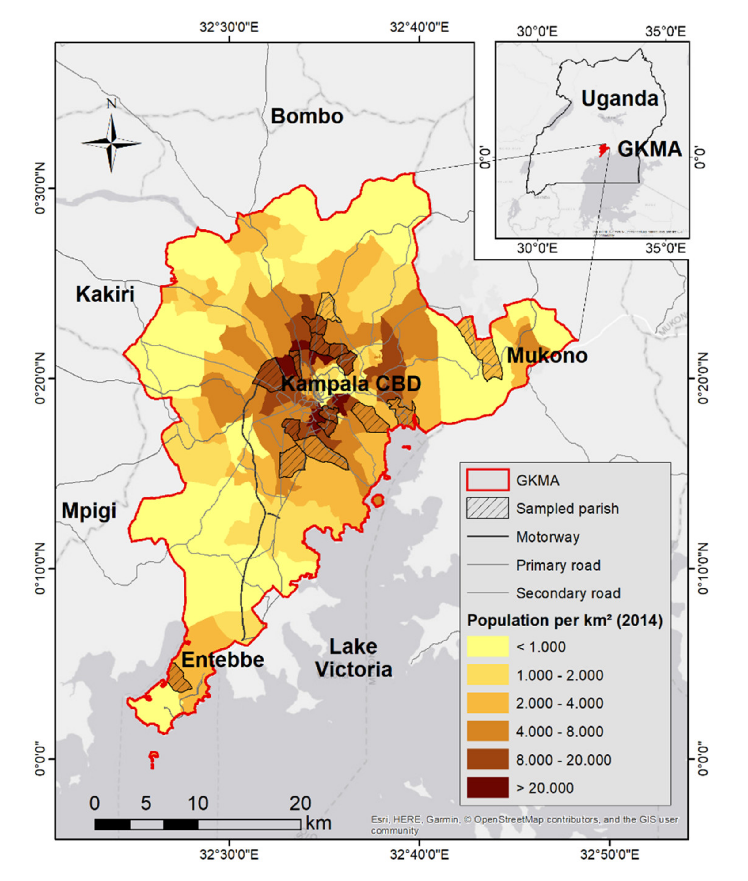
2.1. Study Area: The Greater Kampala Metropolitan Area

Aiming at analyzing socioeconomic dynamics, the Greater Kampala Metropolitan Area (GKMA) in Uganda has been selected as a case study (Figure 1). The study area is positioned at the northern shore of Lake Victoria and encompasses an area of about 1026 km2. The smallest administrative unit (SAU) for which census data are available in Kampala is the parish. The GKMA as presented in Figure 1, comprises 171 parishes. Kampala is a representative case for many SSA cities, because it is characterized by a recent and very rapid population increase of over 5% per year, resulting in social segregation and an inefficient city layout [2,30]. In 2015, the inner city was inhabited by over 1.9 million people, which is more than two-fold the population in 1995 [1]. Recent population estimates for the entire GKMA depend on how the area is demarcated, and range from 3.13 million [31] to over 4 million [32]. Due to the rapid horizontal expansion of the capital, the urban agglomeration of Kampala now includes former satellite towns such as Mukono and Entebbe [33] (Figure 1). The exponential growth of Kampala’s population is likely to continue in the future for two reasons. First, many rural dwellers are attracted to employment opportunities in the capital city and decide to migrate [34,35]. Second, with Uganda’s total fertility rate at 5.91 children per woman [36], natural population growth will add to the population increase of the city.
Kampala is situated in a hilly area. Wealthy inhabitants generally choose to build their homes on hilltops while slums have developed in low-lying, flood prone wetlands [2,7,9]. The informal inhabitants of these wetland areas often depend on urban farming practices for their livelihood. It is often assumed these agricultural activities are a remnant of the “rural lifestyle” new migrants to the city used to have [37]. Even though Kampala’s inhabitants and their livelihoods have been studied from multiple perspectives, household typologies have traditionally focused on income and ownership, as well as the involvement in urban agricultural activities [2,14,37]. In this paper, we argue that while these factors are imperative, it is essential to include a broad spectrum of socioeconomic variables to create household typologies.

2.2. Household Surveys

To obtain a better understanding of socioeconomic patterns and their location characteristics, 541 households were interviewed based on a convenience sample in the GKMA in 2019. Information was gathered on a total of 2487 individuals within the households. A mixed team of six interviewers from KU Leuven and Makerere University carried out the surveys. The households were approached at their homes in 15 contrasting parishes (the SAU) of the GKMA (Figure 1). We aimed to survey households at SAU that are contrasting both in terms of socioeconomic dynamics, as well as their geographic location within the GKMA. For more information on the sampling strategy, please refer to Appendix B. Informed verbal consent was registered from the interviewee, after which a 50-min survey was conducted. Survey responses and point locations were collected digitally on a mobile phone device or tablet, using the Open Data Kit Collect application (version 1.24.1). The present study uses three subsections of the full household survey: household characteristics, neighborhood characteristics, and income and ownership. The survey protocol was approved on 19 June 2019 (approval number G-2019 06 1664) by the KU Leuven Social and Societal Ethics Committee (SMEC).

2.3. Socioeconomic Survey Data Clustering

To convert the sampled household survey data into socioeconomic representations for the whole population of the GKMA, a disproportional upscaling method is applied. Households are clustered into distinct, more homogeneous groups rather than considering the sampled averages representative for all inhabitants [38]. This clustering of the data was carried out in R (version 3.6.2) using the k-prototypes algorithm, as this was developed specifically for clustering of mixed numerical and categorical data [39]. The “clustMixType” package for R [40] was used to create socioeconomic clusters (SEC) based on the survey data. Since this clustering tool does not tolerate missing values, empty values were imputed through a multiple imputation method using the “missForest” package for R [41]. 16 surveys were excluded from clustering, as these were inadequately sampled. These cases were not systematically different from sampled cases in demographics. Appendix C contains a detailed missing data analysis, concluding that data are missing at random. This way, 525 households were included in the k-prototypes clustering.
71 socioeconomic variables (summarized in Table 2) were included that can be linked to residential choice in Kampala [14], and, thus, the dwelling exterior. These variables can be subdivided into three collections: household characteristics, neighborhood characteristics and variables related to income and ownership [13]. In absence of detailed census information, four clusters were chosen because this enables comparison and validation with recent research on the socioeconomic segregation of Kampala [2,14,16]. The output of the clustering method will consequently assign a SEC to each of the interviewed households. To avoid the result of a small, non-representative cluster (e.g., of a wealthy elite), the k-prototypes method parameters were calibrated to produce four similarly sized clusters. A Welch two-sample t-test is carried out in R for each cluster compared to the rest of the dataset to visualize cluster differences. Categorical variables were transformed to numerical for t-value calculations: e.g., yes (1), no (0); or agree (1), neutral (0.5) and disagree (0).

2.4. Remote Sensing Classification of Residential BUA

A remote sensing classification was carried out for the entire study area to upscale the socioeconomic data gathered at household level. Therefore, unlike conventional remote sensing analyses, we aimed at distinguishing four land use classes within the residential built-up area (BUA): villa housing, large housing, small housing and slum housing (Figure 2). The villa housing is characterized by large, clearly demarcated plots of over 1500 m2 on a regular road grid. The villas have a BUA of over 250 m2. All villa housing plots have a garden with vegetation cover, and some have a swimming pool on site. This housing typology may be confused with some of the larger hotels and resorts in touristic areas. The large housing consists of residences of about 150 m2 with a semi-regular street layout. These homes usually have a garden, with average plot sizes over 400 m2. The small housing residential class consists of smaller dwellings of under 100 m2. Nonetheless, these residences still have access to a small garden area with plots of about 200 m2. The slum housing typology can be considered to be non-permanent structures of about 50 m2 or less, with a highly irregular street layout. Slum housing rarely has access to a nearby garden. These four residential BUA classes respectively correspond to housing typology types A, B, C and D as recently defined by [14]. Alongside these four categories, we defined “industrial”, “water” and “other”. The latter mainly comprises of (non-garden) vegetation including grass, forest, and swamps.
We conducted a comparative study of various classification methods that are readily available in popular GIS software packages. The main criterion in this comparative study was the classifier accuracy for the residential built-up classes. Examined methods include principal components analysis, ISO cluster unsupervised classification, and maximum likelihood supervised classification. The satellite imagery should be appropriate for the desired purpose and study area. Although typically, higher-resolution satellite imagery results in better classifications, the image resolution should fit the average plot size in the study area [12], to include the possible influence of garden vegetation and swimming pools. Open access imagery is recommended for analyses targeting urban development issues. In addition, the time at which the image was taken should closely correspond to the time at which the household surveys and most recent national census were carried out. For these reasons, all methods were tested on recent Sentinel-2 and Landsat-8 imagery.
The pixel-based, maximum likelihood (ML) supervised classifier performed most satisfactory for the purposes of this research. The ML method is based on the Bayesian probability theory using the variance and covariance data of the training pixel signatures to make an estimation of the probability that a pixel belongs to a certain class [42]. The prior probability used corresponds to the amount of training pixels selected for each class (sample probability). ML is a relatively simple and well-known method in remote sensing, and was applied for a Landsat-8 image in ArcGIS (version 10.7.1). The Landsat-8 satellite image covering the GKMA (path 171, row 60) was chosen based on its recent date (February 2020), minimal cloud cover (< 3%) and suitable resolution (30 m). In addition, the Landsat-8 images are available open-source and atmospherically corrected via USGS.
The imagery used for visual selection of training and validation pixels are Maxar, available via Google Earth or the ArcGIS imagery base layer, of 0.3 m resolution (Figure 2). In addition, Google Streetview and field observations were consulted to ensure the quality of the training and validation data. The training data are small polygons of approximately 85 pixels each, for which the land cover class is known. Figure 2 shows how typical variations in residential BUA can be detected and selected as training or validation areas with the aid of the Maxar high-resolution imagery. Adhering to the guidelines by [42], 1829, 4894, 4307, and 3905 training pixels were selected on the Landsat-8 image for the slum, small, large, and villa residential housing classes, respectively. For validation, 120 pixels per land use class outside of the training sites were selected. Based on the validation data, we generated an error matrix. Classification accuracy was assessed using the percentage correctly classified (PCC) and the Kappa Index of Agreement (KIA) [43]. In addition, we generated a confidence raster showing the spatial distribution of the ML classification certainty.

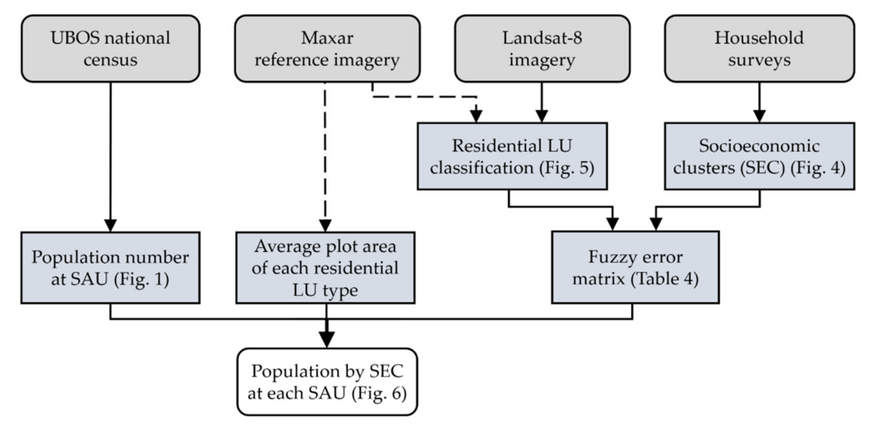
2.5. Upscaling Socioeconomic Clustered Data Using the Remote Sensing Classification

Finally, a fuzzy error matrix (Table 3) was generated to evaluate to what extent the ML classification correlates to the locations and SEC of the surveyed households. In a traditional error matrix, classified pixels are compared to validation data on the diagonal only. However, the land use classes described in this study are not clear-cut. The spectral signatures of these classes will not be clearly distinguishable as these are all built-up, residential land use. Therefore, for certain residential groups, we consider one adjacent class to be “correctly classified” or (potentially) matching in the fuzzy matrix [43]. For example, without any knowledge of their dwelling exterior, a household in a high income cluster would likely reside in either a villa (i = 1) or in large housing (i = 2). In this case, we assume more established households have more location-specific knowledge [28] and have had the time to adapt or enlarge their home exterior. Depending on the geographical context, the proposed (potentially) matching pixels in the fuzzy error matrix in Table 3 can be adapted to represent the level of visual housing segregation.
The UBOS [31] national census population per parish (density shown in Figure 1) was merged with an OpenStreetMap spatial layer to geographically display the population at parish level for the entire GKMA. This parish-level population number is then reclassified based on the error matrix to display what percentage of the parish population belongs to each SEC. Depending on the case study and the amount of available survey locations, it can be decided to reclassify the population at the SAU using either the entire error matrix, or only those cells considered to be (potentially) matching. In this study, all matching or potentially matching values were considered for this reclassification. Wealthier households in villas reside on larger plots of land, and therefore have a lower population density. Hence, the average plot sizes for each residential housing type in Kampala as described in Section 2.4. were used for conversion. Figure 3 summarizes the workflow for this study.

3. Results

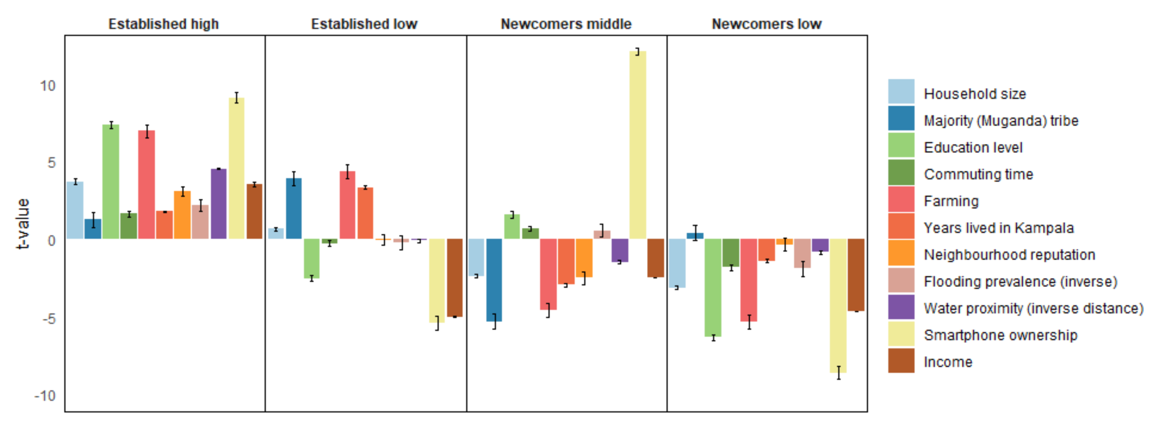
3.1. Socioeconomic Clustering

Using the k-prototypes method, 525 surveyed households in Kampala are subdivided into four distinct SEC, subdivided by income (“high”, “middle”, “low”) and embeddedness in Kampala (“established” versus “newcomers”). Figure 4 displays the t-values for a selection of 10 variables (out of a total of 71) which capture the household typology. Higher t-values are linked to a higher standard of living as the inverse of “undesirable” variables (flooding prevalence, distance to nearest water source) is shown.
The first group consists of 143 households, the “established high” (EH). They are the most affluent inhabitants of the GKMA with a median monthly income per person of 207,000 UGX. EH households are the largest of the dataset, with an average of 6.4 persons. 64% of EH households indicate they belong to the majority tribe in Kampala, the Muganda. These households are well-established within the urban dynamic: most spent over 15 years in Kampala and 78% engage in urban agriculture for (part of) their livelihood. They live in neighborhoods with a good reputation and low flooding risk. Most households in this first group are highly educated at tertiary level, which is reflected in relatively long commuting times to their place of employment. 89% own a smartphone, and nearly everyone in this group has water tapped inside their home.
The second group can be defined as the “established low” (EL) class, containing 97 households. This group is characterized by a low median income per person of 87,500 UGX and they have resided in Kampala for a long time (median 19 years) with relatively large household sizes. 77% of EL households are Muganda. They live in neighborhoods with an average reputation and flooding prevalence. This group is educated at lower secondary level, has poor access to technology (30% own a smartphone) and fresh water either inside their home or at less than 20 m distance. For their livelihood, this group lives rather near their workplace and the majority (72%) engages in urban agriculture.
With a median income of 131,000 UGX, the third SEC of 111 households is referred to as “newcomers middle” (NM). This SEC entails mostly new migrants, with the majority having resided in Kampala for less than 10 years. This is reflected by their limited engagement in urban agriculture (28%). NM households are educated at higher secondary level, and nearly all (95%) own a smartphone. Nonetheless, despite their middle-range income, they live in neighborhoods with a poor reputation. This suggests that due to their recent migration to Kampala, their choice of place of residence was limited [14]. These families are comparatively small (median of 4 persons), and usually do not have a water tap inside their residence. The majority tribe are underrepresented in this group with only 32% of households.
Lastly, the “newcomers low” (NL), a cluster with 174 households, are similar to the third group with some exceptions. Most (60%) are of the majority Muganda tribe. Their monthly household income is low, with a median of 99,500 UGX, while their households are similar in size to the NM. The individuals do not commute far (median 22 minutes), suggesting they live on temporary employment daily. In contrast with the NM, the NL are usually educated at primary or lower secondary level and only 24% owns a smartphone.

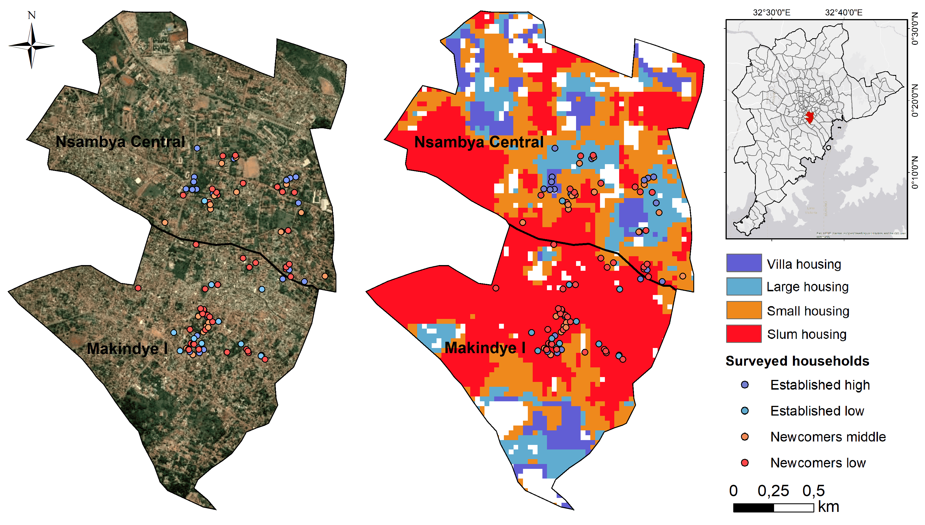
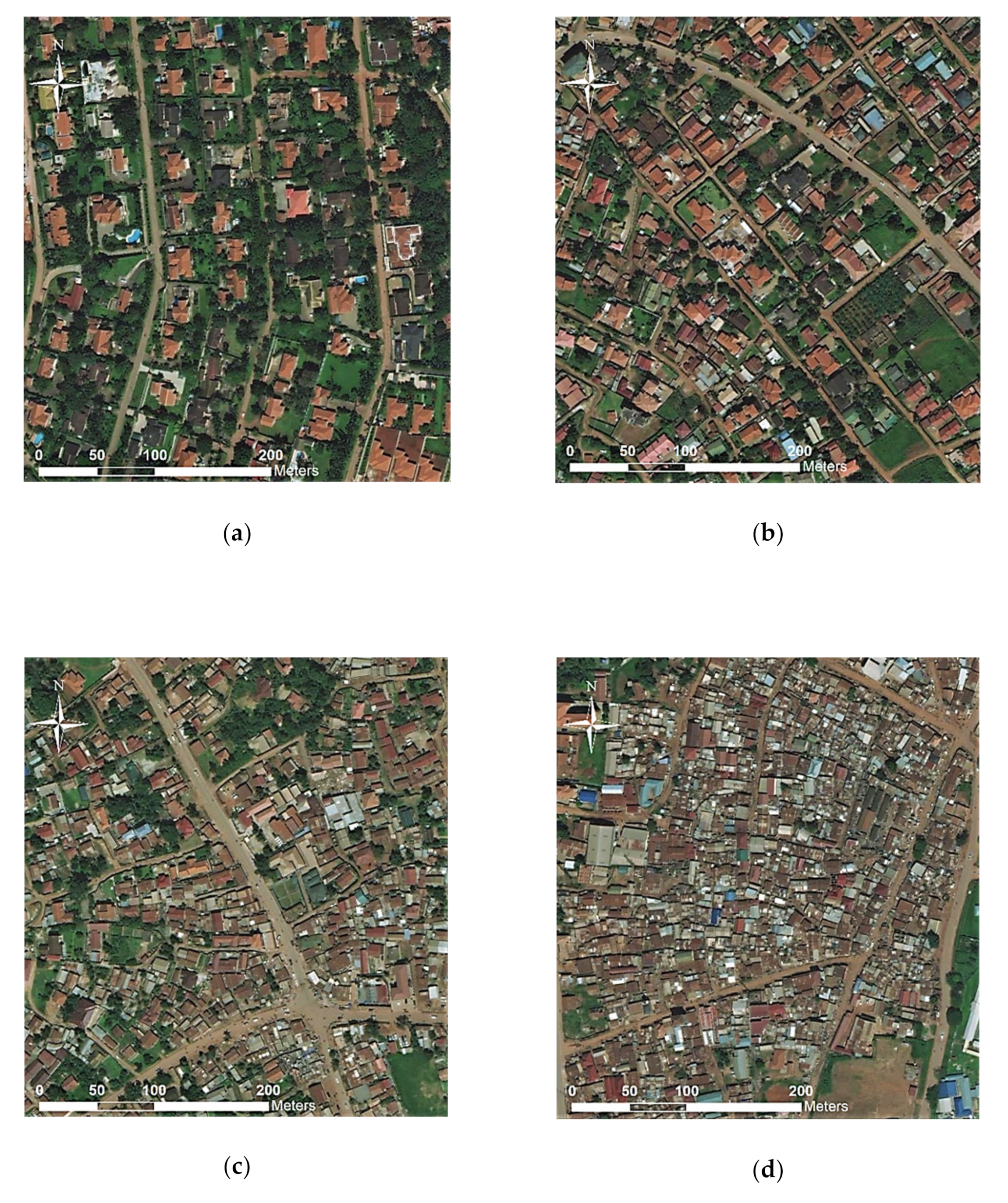
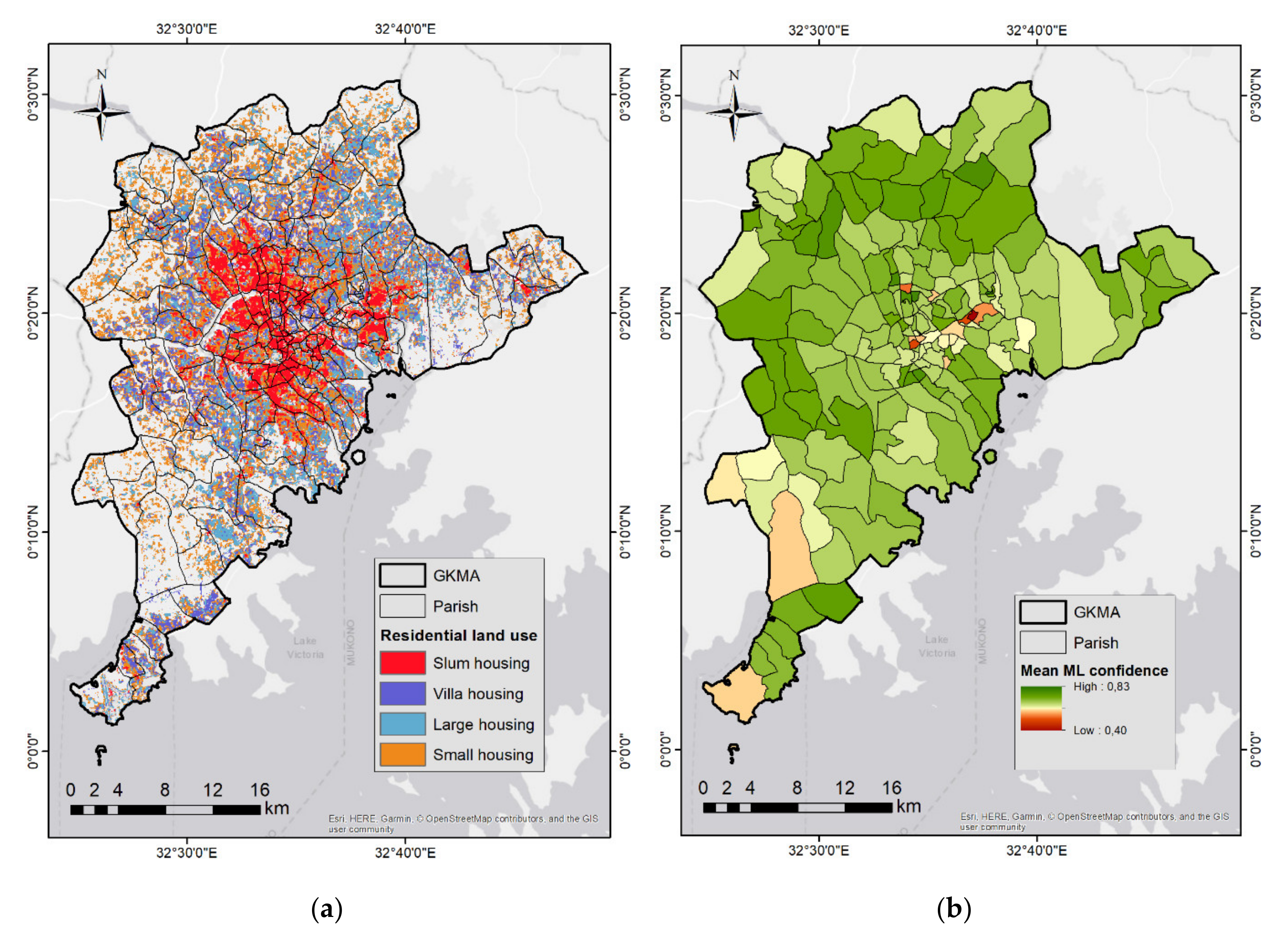
3.2. Residential Land Use Classification

Figure 5a shows the result of the ML classification, distinguishing four land use classes within the residential BUA: villas, large housing, small housing, and slums. The emerging pattern shows the slum housing is chiefly located around the central business district (CBD). Although some clusters of villas exist on the hilltops in the city, most are located on the outskirts or towards the touristic areas in Entebbe. In many locations, a gradient is visible where a cluster of slum housing is found adjacent to small residences, which in turn neighbor areas with large housing, which are located next to villas.
Figure 5b displays the mean ML confidence of pixels classified as residential for each SAU. The suburban areas were classified with the highest confidence. Some smaller parishes within the inner city have a low mean confidence (< 0.5), which can be attributed to the presence of undefined land use classes (currently “other”) such as parks and infrastructure. The mean confidence for the entire study area is 0.7. Furthermore, the ML result was validated with 120 control points per class and resulted in a PCC of 61.5% and a KIA of 0.575, i.e., when taking into account only the diagonal of the classic error matrix (Appendix A). The slum housing classification performed the best, while the classification of the large, small, and villa residential classes is more ambiguous. The relatively low overall PCC and KIA values are largely due to this fuzziness in the middle-to-high income residential BUA. This is not surprising considering that with large gardens and swimming pools, the villa housing class consists of the largest spectral heterogeneity.
The correlation between the SEC resulting from the survey data and the output of the ML classification is displayed as a fuzzy error matrix in Table 4. Values indicated with * (PCC 52.7%; KIA 0.377) can be considered to be matching based on income group and “newcomer” or “established” status. When the locations considered to be potentially matching (**) are also included, the correlation accuracy goes up to a PCC of 72.8% and a KIA of 0.594. Producing the same fuzzy error matrix for the income variable only, results in lower accuracies with a PCC 47.5% and KIA 0.328 for the matching values. This further validates this approach, showing that a broad spectrum of socioeconomic variables shows a stronger upscaling potential than income only.

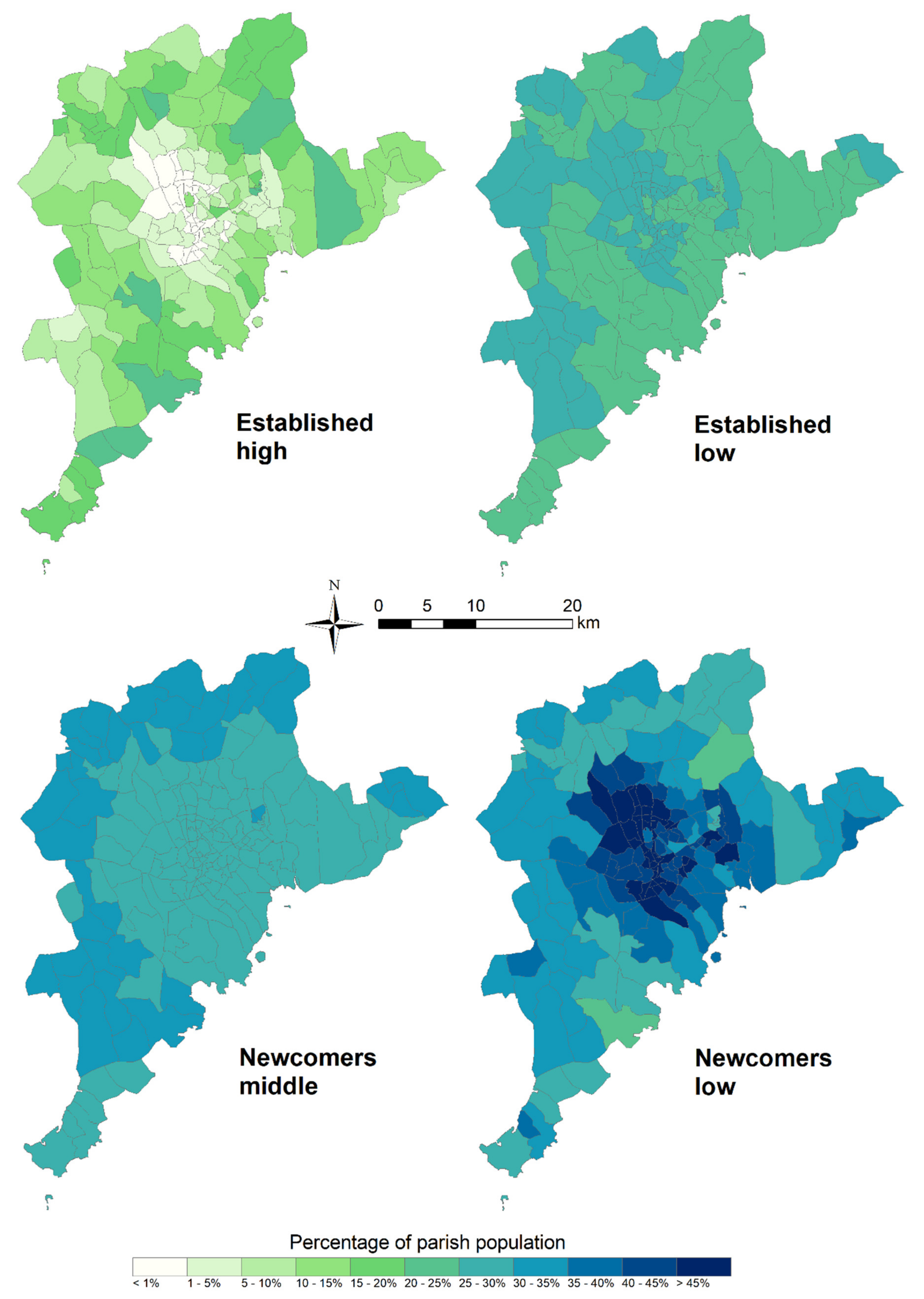
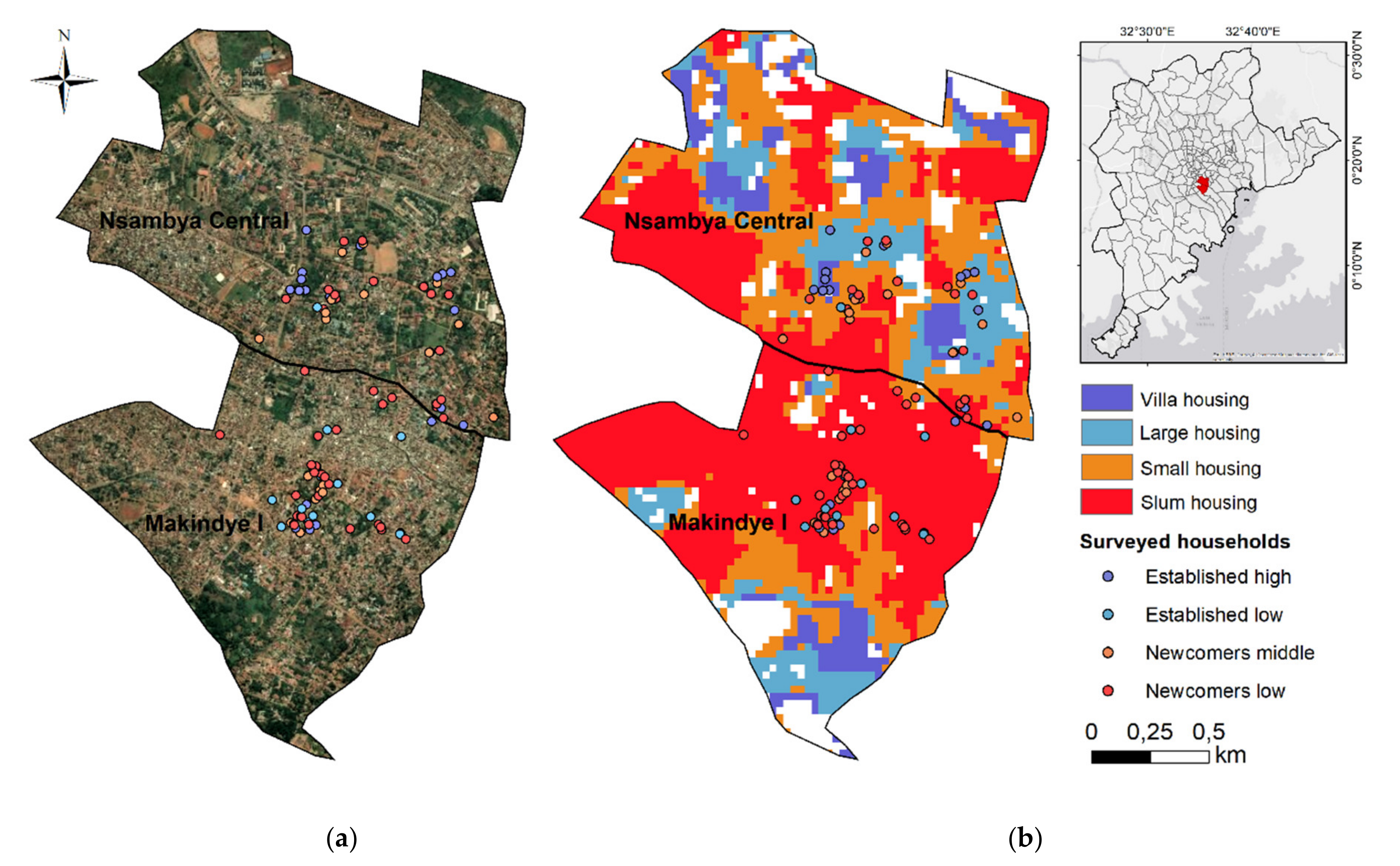
3.3. Socioeconomic Population Maps

The matching and potentially matching values in Table 4 were used to reclassify the parish population in the GKMA according to these proportions. In other words, we upscale the household survey findings to represent a portion of the census population number at each SAU. We assume the population density is different for each housing type as described in Section 2.4.: small homes are located on plots four times as large as slums, large housing plots are eight times as large as slums, and villa plots are 30 times larger than slums. Figure 6 shows the resulting percentage of the parish population taken up by each SEC. The EH is the smallest group: they never consist of more than 25% of the total population of a parish. They live in the direct outskirts of Kampala city, as well as on some of the hillier areas within the inner city. The touristic areas around Entebbe and the newly constructed motorway are also classified as having relatively many (> 20%) EH inhabitants, though this could be due to the presence of large hotels. The EL, on the other hand, are spatially very well spread out over the GKMA, with about one fourth of the population of each parish being part of this SEC. The NM are also scattered around Kampala and its surroundings, but make up a slightly larger share of the parish population on the edges of the GKMA, along with the EL. The NL are present everywhere as well, but are most highly concentrated (> 45%) in the densely inhabited inner city of Kampala.
Most parishes in the densely inhabited inner city of Kampala are thus inhabited predominantly by NL, with an approximately even share of EL and NM population. This implies that either the city of Kampala is not as socioeconomically segregated as hypothesized, or that this segregation occurs at the sub-parish scale. Figure 7 shows how the ML classifier performs at sub-parish parish scale for two adjacent parishes in central Kampala: Nsambya Central and Makindye I. By visual comparison, the classifier performs well. For instance, larger residences with gardens, visible on the Maxar imagery throughout Nsambya Central and in the southern areas of Makindye I are correctly detected as villa housing. Combined, 100 georeferenced surveys were carried out in these parishes. Table 5 shows how these survey points correlate with the ML classifier. According to this fuzzy error matrix, the classification performs best for small housing or slum-type residential areas, as these are the dominant land use in the city center.

4. Discussion

4.1. Which Socioeconomic Groups Are Present in the City?

The household survey responses were clustered into four socioeconomic groups (Figure 4): the “established high” (EH), “established low” (EL), “newcomers middle” (NM) and “newcomers low” (NL). The Agent-based simulation of Social Segregation and Urban Expansion (ASSURE) [2,16] also defines SEC in Kampala, though their focus is mainly on income. This section will discuss the similarities and differences between the outcomes both studies. The EH in this study are similar to their “rich” group in terms of income, livelihood, and household size. The EL group is equivalent to the “poor” group. Although their income is low, the EL are rooted within the urban atmosphere of Kampala. Compared to their [2,16] clustering, the NM group is the most similar to their “middle income” respondents. A large part of the income of NM might be sent to other areas as remittances, explaining their relatively high income but low standards of living [45]. Nonetheless, as information on remittances was not included in the household survey, this hypothesis cannot be confirmed. The NL can be compared to the “extreme poor” cluster in [2], due to their low income and low standard of living.
Next, we upscaled the socioeconomic clustering to the entire GKMA at the level of the SAU (parish) in Figure 6. To validate this approach, we visually compare the result in Figure 6 with the socioeconomic segregation map by [2] (p. 2385). This comparison shows a clear parallel: the poor and extreme poor SEC are the largest in most parishes, while the wealthier urban residents tend to locate on hilltops in the inner city, or in well-connected suburban areas [2,14]. Some confusion is present between the locations of the NM (“middle”) and NL (“extreme poor”). The NL are concentrated mainly in the inner city. This is not surprising, as other research in SSA cities show new migrants who can afford it tend to migrate towards the city center first, in search of employment. However, because Kampala is a polycentric city, newly migrated households (of all income groups) are observed to be spatially spread out, thus not displaying any discernible “spaces of arrival” [14,46]. The research project by [2,16] gathered data between 2010 and 2013, which in a rapidly growing city as Kampala means these dissimilarities could be attributed to changing social dynamics. However, as their clusters are defined somewhat differently, and they do not specify how exactly they estimate the locations of these socioeconomic groups, this comparison should be interpreted with caution. As the results for Kampala closely correspond to preceding research in the GKMA, the rapid horizontal expansion of the city is likely to continue via the same socioeconomic dynamics in the future.

4.2. How Can Household Surveys Be Upscaled Using Remote Sensing to Locate Where Socioeconomic Groups Are Residing in the Greater Metropolitan Area?

The socioeconomic typologies found by clustering the household survey responses were upscaled to the entire metropolitan population of Kampala by directly comparing their locations to a ML classification of Landsat-8 imagery. The workflow is depicted in Figure 3. This comparison was by means of a fuzzy error matrix, where only the (potentially) matching pixels were used for upscaling. To do so, an estimate is needed for the amount of space (e.g., plot areas) taken up by each housing type. The results in the fuzzy error matrix (Table 4) confirm our hypothesis, indicating that household income is not the only predictor of housing infrastructure in the GKMA [14]. The newcomer groups show the strongest correlation with the small housing and slum housing locations. Oddly, the EH are occasionally located within areas classified as slum housing. Nonetheless, the limited number of household locations that coincide with larger homes (7.3%) or villas (5.3%), makes it challenging to judge the upscaling method for the EH. To an extent, the fuzzy error matrix in Table 4 validates the hypothesis that remotely sensed patterns of segregation are a reflection of the SEC residing there. However, we conclude that socioeconomic household characteristics are much less spatially clustered in the GKMA than the housing typologies. Our findings therefore confirm the results of previous studies in Kampala [14,16].
The added value of the method presented in this study is in its combination of two relatively well-known and straightforward methods. Both in the socioeconomic clustering of household surveys as in the residential land use classification, it is clear that segregation in Kampala occurs at sub-parish level (Figure 7). When urban land use classifications are compared with socioeconomic data points, this usually occurs at a spatially aggregated level, e.g., the SAU. This is due to the availability of socioeconomic information often being limited to census data, which cannot be disclosed at household level [12]. In the context of urban SSA, detailed socioeconomic census data are often absent at the scale of the SAU. When dynamics of segregation take place at a finer spatial resolution than the SAU, it is, therefore, favorable to apply a method of pixel-based validation.
Clustering analyses of survey data are common in both social sciences [38] and urban systems modelling studies [2]. Likewise, remotely sensed population base maps can be used for urban planning and resource allocation [47]. Combining these methods, however, should be intuitive and straightforward, so that its application is justified in many fields. Most GIS software provide uncomplicated tools to compare point values with underlying raster cell values, which can be used to create a fuzzy error matrix. We propose this method to avoid that modelling efforts rely only on estimations [2] or interpolations at local level [14] for their socioeconomic population base maps. An additional advantage is that the upscaling of household surveys to wider study areas would facilitate the availability of socioeconomic population base maps, which supersedes the need to share extensive datasets containing sensitive information.

4.3. Limitations

There are limitations to the presented research. We use quantitative data to demonstrate relationships between many variables, yet this does not explain possible causalities. Further research will be required to confirm or discard propositions as to why these relationships are found. Additionally, the SEC were estimated based on a convenience sample of households, and therefore the results of the cluster analysis should not be interpreted as generalizable to other contexts. Hence, future studies should replicate the cluster analysis with a larger probability sample.
This study would benefit from more geographically spread out household survey locations as this would increase the accuracy of the ML comparison. Preferably, the geographical reach of the survey sample would cover the entire study area. Another spatial constraint of this study is that household survey sites were included as point locations, rather than as polygons, as done by [48]. As with increased household surveys, including the property areas of sampled households could have resulted in a larger number of validation pixels. However, this was indirectly dealt with as Landsat-8 imagery of 30m resolution (1 pixel = 900 m2) was used, which more than reflects the area of 331 m2 taken up by an average household in the GKMA [2].
As mentioned, different remote sensing classification methods or household survey clustering methods can be combined, which might result in different socioeconomic population base maps. A drawback of the proposed method is that there are errors associated with both the remotely sensed land use classification, and with the socioeconomic clustering of surveys. Combining both methods implies that there is an inevitable error propagation in the resulting socioeconomic layout of the city. With careful selection of training pixels and adequate spatial survey sampling these errors can be minimized. Nonetheless, the output should be interpreted as an overall pattern of the urban socioeconomic geography rather than as an accurate measure of segregation.

5. Conclusions

This paper proposes an intuitive methodology to directly compare and combine household-level socioeconomic survey data with a remotely sensed classification of built-up residential areas. We demonstrate that a combination of survey and remotely sensed data is more powerful than either of these approaches in isolation. Although we applied a k-prototypes clustering method to the survey responses and a maximum likelihood classifier to Landsat-8 satellite imagery, future work could evaluate a different combination of techniques to further validate this approach. Upscaling the survey findings to the GKMA suggests socioeconomic segregation in the city occurs at sub-parish level. In the inner city, the largest group are the “newcomers low”, while share of the parish population belonging to the “established low” or “newcomers middle” clusters is often roughly equal. This stresses the need for residential land use classifications that are validated with survey information at spatial resolutions that exceed the SAU. The results for Kampala correspond to previous research carried out in the area, suggesting the rapid horizontal expansion of the city is continuing via the same socioeconomic dynamics. Unless policy action follows these insights, a business-as-usual scenario is therefore likely for Kampala in future analysis or modelling efforts.

Author Contributions

Conceptualization, L.-M.H. and A.V.R.; methodology, L.-M.H. and J.R.; software, L.-M.H. and S.V.E.; validation, L.-M.H., J.D. and J.R.; formal analysis, L.-M.H. and J.R.; investigation, L.-M.H., S.V.E., J.R. and data collectors mentioned in the acknowledgements.; resources, L.-M.H. and S.L.; data curation, L.-M.H., S.V.E. and J.D.; writing—original draft preparation, L.-M.H.; writing—review and editing, all contributors; visualization, L.-M.H.; supervision and mentoring, A.V.R. and S.L.; project administration, A.V.R., P.H.V., J.D. and S.L.; funding acquisition, L.-M.H., A.V.R., P.H.V. and S.L. All authors have read and agreed to the published version of the manuscript.

Funding

This research was funded by LEAP-Agri and Fonds Wetenschappelijk Onderzoek (FWO) Vlaanderen (grant number 11C6120N).

Acknowledgments

The authors would especially like to thank our colleagues and data collectors from the Urban Action Lab at Makerere University, namely Teddy Kisembo, Judith Mbabazi, Gloria Nsangi, Hakimu Sseviiri, and Disan Byarugaba. A KU Leuven master student also participated in data collection: Desmond Khisa Situma. We would also like to thank the local council leaders of the sampled parishes in Kampala for their guidance and assistance on the field. This work was supported by the Food4Cities project, funded by the LEAP-Agri program of the European Union. This work is part of the first work package in project 11C6120N: “Spatial analysis of food systems transformations in rapidly growing African cities”, funded by Fonds Wetenschappelijk Onderzoek (FWO) Vlaanderen.

Conflicts of Interest

The authors declare no conflict of interest. The funders had no role in the design of the study; in the collection, analyses, or interpretation of data; in the writing of the manuscript, or in the decision to publish the results.

Appendix A

Table A1. Error matrix showing how the maximum likelihood classification performed compared to the validation control points. Correctly classified (*) accuracy: PCC 61.5%, KIA 0.575. Fuzzy (**) accuracy: PCC 77.3%, KIA 0.743.
Validation Points
Pixel Value Villa
Housing
Large
Housing
Small
Housing
Slum
Housing
IndustryWater OtherTotal (Pixels)
ML classificationVilla housing49 *23 **14260599
Large housing22 **48 *13 **01306102
Small housing2834 **48 *3 **1409136
Slum housing2637 **107 *1401167
Industry100150 *0254
Water00000118 *0118
Other1898723297 *164
Total (pixels)120120120120120120120840

Appendix B

A convenience sampling method was adopted on the field. We aimed to survey households at small administrative units (SAU) that are contrasting both in terms of socioeconomic dynamics, as well as their location within the study area. The sampled SAU were selected based on prior geographic research on socioeconomic dynamics (Vermeiren et al., 2016) combined with local expert consulting with colleagues at Makerere University. Between July and December 2019, six interviewers approached homes in 15 contrasting parishes (the SAU) of the Greater Kampala Metropolitan Area (GKMA, Figure 1). Additional factors considered for selection of SAU were transport logistics and safety for the interviewers. A possible selection bias could therefore occur in terms of neighborhood accessibility. Households located deep within areas that are considered to be unsafe or difficult to access were not included in sampling.
Sample size was therefore constrained by practical access to the SAU. However, as a guideline to target sample size we calculated that with a desired confidence interval of 95%, the sample size of 541 households results in a margin of error of 1.97% based on Cochran’s [49] sample size formula for estimating prevalence (Equation (A1)):
n 0 =   Z 2 p 1 p e 2
where:
  • n is the sample size (541 households, with 2487 individuals).
  • p is the population proportion (assumed at 0.5 for complete uncertainty).
  • Z the Z-score (1.96 for a confidence interval of 95%).
  • e is the error margin (1.97%).
Within the SAU, households were selected using a snowball strategy where a local council representative, after giving their informed consent, led the interviewers to households and assisted in explaining the purpose of the study. For this reason, households within a selected SAU all needed to be within walking distance from each other. The final sample size was 541 households. Information was gathered on a total of 2487 individuals within the households. This sample size calculation method is based on similar approaches used for matching land use with socioeconomic factors [50] and food security [51].

Appendix C

Missing data were assessed using base functions and the missForest [41] and irr [52] packages in R statistical software. Overall, 3.04% of observations were missing from the dataset used for cluster analysis. Missing data were imputed through a multiple imputation method. All variables used in the clustering analysis were used to impute missing data. A nonparametric random forests multiple imputation method, suitable for mixed numeric and categorical data, was implemented in the R package missForest [41]. The dataset reached the stopping criterion after 6 iterations. The imputed values showed high coherence with a low normalized root mean squared error for continuous variables (NRMSE = 0.51) and a low proportion of falsely classified categorical variables (PFC = 0.12).
Missing data from participants were assessed to decide whether each participant had been adequately sampled. Missing data analysis was performed as part of a larger data cleaning procedure, in which logic tests were applied to assess the reliability of participant responses (for example, if household-level information did not match household roster data). The total proportion of missing data per participant was then calculated to include both non-responses and responses deemed ineligible due to testing logic.
Participants had an average of 4.25% missing data (SD = 10.91%, range = 0-95%). A threshold of 37% missing data per participant was selected for further investigation. This threshold was chosen to minimize the number of participants that would be excluded, while balancing adequate sampling per participant (see Figure A1).
Figure A1. Number of participants that would be excluded at each missing data threshold. Note change point at 37% missing data.
Remotesensing 12 03468 g0a1
Sixteen participants (2.96% of the total sample of 541 participants) had more than 37% missing data. These cases were examined to discover whether anything unusual had happened during the recruitment and/or survey administration. On examination it appeared that these participants had abandoned the survey partway, perhaps due to its length. Since these participants had systematically answered the initial survey questions and not the later ones, we concluded that these cases were inadequately sampled. These cases were therefore removed from the dataset. We do not expect that removing these cases should have any effect on the substantive results of this study for two reasons. First, they represent a small percentage of the overall sample (< 3%). Second, these cases were not systematically different from sampled cases in demographics: missing data per participant was not significantly predicted by language, F (28, 507) = 1.31, p = 0.138, income, F (1, 434) = 0.43, p = 0.514, or household size, F (1, 539) = 0.59, p = 0.441. Therefore, removing these cases would not bias the parameters estimated from the data in the analysis, and should have no effect on the validity of the study results.
Missing data from variables were assessed to decide whether each variable had been adequately assessed across the sample. Variables had an average of 3.08% missing data (SD = 3.60%, range = 0-19.41%). The highest percentages of missing data were found for average commuting time (12.01%) and monthly income (19.41%). A series of separate variance t-tests did not reveal any systematic patterns between the missing data in these variables and the values of other variables in the dataset related to wealth or travel method, including ownership of a car, van, or motorcycle (min. p = 0.110, p = 0.695, and p = 747, respectively). Results therefore suggest that these data were missing at random.
Based on the results of the separate variances t-tests, and the low overall proportion of missing data, we concluded that subsequent to removing the cases with >37% missing data, there should be no relationship between the probability of missing data, and the expected value of that missing data. Therefore, we conclude that the data are missing at random; that is, the treatment of missing values should not present a problem for the validity of the resulting analysis estimates.

References

  1. UN-DESA. World Urbanization Prospects: The 2014 Revision; United Nations: New York, NY, USA, 2015. [Google Scholar]
  2. Vermeiren, K.; Vanmaercke, M.; Beckers, J.; Van Rompaey, A. ASSURE: A model for the simulation of urban expansion and intra-urban social segregation. Int. J. Geogr. Inf. Sci. 2016, 30, 2377–2400. [Google Scholar] [CrossRef]
  3. Dieleman, F.; Wegener, M. Compact City and Urban Sprawl. Built Environ. 2015, 30, 308–323. [Google Scholar] [CrossRef] [Green Version]
  4. Gaigné, C.; Riou, S.; Thisse, J.F. Are compact cities environmentally friendly? J. Urban Econ. 2012, 72, 123–136. [Google Scholar] [CrossRef]
  5. Smets, P.; Salman, T. Countering urban segregation: Theoretical and policy innovations from around the globe. Urban Stud. 2008, 45, 1307–1332. [Google Scholar] [CrossRef]
  6. Schirmer, P.M.; van Eggermond, M.A.B.; Axhausen, K.W. The role of location in residential location choice models: A review of literature. J. Transp. Land Use 2014, 7, 3–21. [Google Scholar] [CrossRef]
  7. Marx, C.; Johnson, C.; Lwasa, S. Multiple interests in urban land: Disaster-induced land resettlement politics in Kampala. Int. Plan. Stud. 2020, 25, 289–301. [Google Scholar] [CrossRef]
  8. Brousse, O.; Georganos, S.; Demuzere, M.; Vanhuysse, S.; Wouters, H.; Wolff, E.; Linard, C.; van Lipzig, N.P.M.; Dujardin, S. Using Local Climate Zones in Sub-Saharan Africa to tackle urban health issues. Urban Clim. 2019, 27, 227–242. [Google Scholar] [CrossRef] [Green Version]
  9. Kabumbuli, R.; Kiwazi, F.W. Participatory planning, management and alternative livelihoods for poor wetland-dependent communities in Kampala, Uganda. Afr. J. Ecol. 2009, 47, 154–160. [Google Scholar] [CrossRef]
  10. Cohen, B. Urbanization in developing countries: Current trends, future projections, and key challenges for sustainability. Technol. Soc. 2006, 28, 63–80. [Google Scholar] [CrossRef]
  11. Abdul-mumin, A.; Siwar, C. Emerging cities and sustainable global environmental management: Livelihood implications in the OIC countries. J. Geogr. Reg. Plan. 2009, 2, 111–120. [Google Scholar] [CrossRef]
  12. Fox, J.; Rindfuss, R.R.; Walsh, S.J.; Mishra, V. People and the Environment; Kluwer Academic Publishers: Dordrecht, The Netherlands, 2003. [Google Scholar]
  13. Kim, H.; Woosnam, K.M.; Marcouiller, D.W.; Aleshinloye, K.D.; Choi, Y. Residential mobility, urban preference, and human settlement: A South Korean case study. Habitat Int. 2015, 49, 497–507. [Google Scholar] [CrossRef]
  14. Keunen, E. Finding a place to live in the city: Analyzing residential choice in Kampala. Hous. Soc. 2020. [Google Scholar] [CrossRef]
  15. Janusz, K.; Kesteloot, C.; Vermeiren, K.; Van Rompaey, A. Daily mobility, livelihoods and transport policies in Kampala, Uganda: A Hägerstrandian analysis. Tijdschr. Econ. Soc. Geogr. 2019, 110, 412–427. [Google Scholar] [CrossRef]
  16. Vermeiren, K.; Verachtert, E.; Kasaija, P.; Loopmans, M.; Poesen, J.; Van Rompaey, A. Who could benefit from a bus rapid transit system in cities from developing countries? A case study from Kampala, Uganda. J. Transp. Geogr. 2015, 47, 13–22. [Google Scholar] [CrossRef]
  17. Akampumuza, P.; Matsuda, H. Weather Shocks and Urban Livelihood Strategies: The Gender Dimension of Household Vulnerability in the Kumi District Of Uganda. J. Dev. Stud. 2017, 53, 953–970. [Google Scholar] [CrossRef]
  18. Kareem, B.; Lwasa, S. From dependency to Interdependencies: The emergence of a socially rooted but commercial waste sector in Kampala City, Uganda. African J. Environ. Sci. Technol. 2011, 5, 136–142. [Google Scholar] [CrossRef]
  19. Smit, W.; Lannoy, A.D.; Dover, R.V.H.; Lambert, E.V.; Levitt, N.; Watson, V. Making unhealthy places: The built environment and non-communicable diseases in Khayelitsha, Cape Town. Health Place 2016, 39, 196–203. [Google Scholar] [CrossRef] [Green Version]
  20. Linderhof, V.; Dijkxhoorn, Y.; Onyango, J.; Fongar, A.; Nalweyiso, M. Nouricity Progress Report: The Kanyanya Food Challenge—Food Systems Mapping; Wageningen University & Research: Wageningen, The Netherlands, 2019. [Google Scholar]
  21. Battersby, J.; Watson, V. Urban Food Systems Governance and Poverty in African Cities; Battersby, J., Watson, V., Eds.; Routledge: New York, NY, USA, 2019. [Google Scholar]
  22. Fung-Loy, K.; Van Rompaey, A.; Hemerijckx, L.-M. Detection and Simulation of Urban Expansion and Socioeconomic Segregation in the Greater Paramaribo Region, Suriname. Tijdschr. Voor Econ. Soc. Geogr. 2019, 110, 339–358. [Google Scholar] [CrossRef]
  23. Duque, J.C.; Patino, J.E.; Ruiz, L.A.; Pardo-Pascual, J.E. Measuring intra-urban poverty using land cover and texture metrics derived from remote sensing data. Landsc. Urban Plan. 2015, 135, 11–21. [Google Scholar] [CrossRef]
  24. Baud, I.; Kuffer, M.; Pfeffer, K.; Sliuzas, R.; Karuppannan, S. Understanding heterogeneity in metropolitan india: The added value of remote sensing data for analyzing sub-standard residential areas. Int. J. Appl. Earth Obs. Geoinf. 2010, 12, 359–374. [Google Scholar] [CrossRef]
  25. Taubenbock, H.; Wurm, M.; Setiadi, N.; Gebert, N.; Roth, A.; Strunz, G.; Birkmann, J.; Dech, S. Integrating remote sensing and social science. In Proceedings of the 2009 Joint Urban Remote Sensing Event, Shanghai, China, 20–22 May 2009; pp. 1–7. [Google Scholar] [CrossRef]
  26. Sabiiti, E.N.; Katongole, C.B. Urban Agriculture: A Response to the Food Supply Crisis in Kampala City, Uganda. In The Security of Water, Food, Energy and Liveability of Cities; Maheshwari, B., Purohit, R., Malano, H., Singh, V.P., Amerasinghe, P., Eds.; Springer Science+Business Media: Dordrecht, The Netherlands, 2014; pp. 233–242. [Google Scholar]
  27. Hall, O. Remote sensing in social science research. Open Remote Sens. J. 2010, 3, 1–16. [Google Scholar] [CrossRef] [Green Version]
  28. Wentzel, M.; Viljoen, J.; Kok, P. Contemporary South African migration patterns and intentions. In Migration and Development in Africa: An Overview; Kok, P., Gelderblom, D., Oucho, J., Eds.; HSRC Press: Cape Town, South Africa, 2006; pp. 171–204. [Google Scholar]
  29. De Soler, L.S.; Verburg, P.H. Combining remote sensing and household level data for regional scale analysis of land cover change in the Brazilian Amazon. Reg. Environ. Chang. 2010, 10, 371–386. [Google Scholar] [CrossRef] [Green Version]
  30. Vermeiren, K.; Van Rompaey, A.; Loopmans, M.; Serwajja, E.; Mukwaya, P. Urban growth of Kampala, Uganda: Pattern analysis and scenario development. Landsc. Urban Plan. 2012, 106, 199–206. [Google Scholar] [CrossRef]
  31. UBOS. Uganda National Population and Housing Census 2014 Main Report; UBOS: Kampala, Uganda, 2014. [Google Scholar]
  32. The World Bank. From Regulators to Enablers: The Role of City Governments in Economic Development of Greater Kampala; The World Bank Group: Washington, DC, USA, 2018. [Google Scholar]
  33. NEMA. Uganda: Atlas of Our Changing Environment; UNEP-GRID: Arendal, Norway, 2009. [Google Scholar]
  34. Herrin, W.E.; Knight, J.R.; Balihuta, A.M. Migration and wealth accumulation in Uganda. J. Real Estate Financ. Econ. 2009, 39, 165–179. [Google Scholar] [CrossRef]
  35. Mukwaya, P.; Bamutaze, Y.; Mugarura, S.; Benson, T. Rural—Urban Transformation in Uganda. In Proceedings of the Understanding Economic Transformation in Sub-Saharan Africa, Accra, Ghana, 10–11 May 2011. [Google Scholar]
  36. UN-DESA. World Population Prospects 2017—Volume II: Demographic Profiles; United Nations: New York, NY, USA, 2017. [Google Scholar]
  37. Atukunda, G.; Maxwell, D. Farming in the City of Kampala: Issues for Urban Management. Afr. Urban Q. 1996, 11, 264–276. [Google Scholar]
  38. Hennig, C.; Liao, T.F. How to find an appropriate clustering for mixed-type variables with application to socio-economic stratification. J. R. Stat. Soc. Ser. C Appl. Stat. 2013, 62, 309–369. [Google Scholar] [CrossRef] [Green Version]
  39. Huang, Z. Extension to the k-means algorithm for clustering large data sets with categorical values. Data Min. Knowl. Discov. 1998, 304, 283–304. [Google Scholar] [CrossRef]
  40. Szepannek, G. ClustMixType: User-friendly clustering of mixed-type data in R. R. J. 2018, 10, 200–208. [Google Scholar] [CrossRef]
  41. Stekhoven, D.J.; Buehlmann, P. MissForest—Non-parametric missing value imputation for mixed-type data. Bioinformatics 2012, 28, 112–118. [Google Scholar] [CrossRef] [Green Version]
  42. Schowengerdt, R.A. Remote Sensing: Models and Methods for Image Processing, 3rd ed.; Elsevier Inc.: San Diego, CA, USA, 2007. [Google Scholar]
  43. Congalton, R.G.; Green, K. Assessing the Accuracy of Remotely Sensed Data, 3rd ed.; CRC Press; Taylor & Francis Group: Boca Raton, FL, USA, 2019. [Google Scholar]
  44. Zandbergen, P.A. Ensuring Confidentiality of Geocoded Health Data: Assessing Geographic Masking Strategies for Individual-Level Data. Adv. Med. 2014, 2014, 1–14. [Google Scholar] [CrossRef] [Green Version]
  45. Van Vliet, J.; Birch-Thomsen, T.; Gallardo, M.; Hemerijckx, L.-M.; Hersperger, A.M.; Li, M.; Tumwesigye, S.; Twongyirwe, R.; Van Rompaey, A. Bridging the rural-urban dichotomy in land use science. J. Land Use Sci. 2020. [Google Scholar] [CrossRef]
  46. Taubenböck, H.; Kraff, N.J.; Wurm, M. The morphology of the Arrival City—A global categorization based on literature surveys and remotely sensed data. Appl. Geogr. 2018, 92, 150–167. [Google Scholar] [CrossRef]
  47. Xu, M.; Cao, C.; Jia, P. Mapping Fine-Scale Urban Spatial Population Distribution Based on High-Resolution Stereo Pair. Remote Sens. 2020, 12, 608. [Google Scholar] [CrossRef] [Green Version]
  48. Pan, W.K.Y.; Walsh, S.J.; Bilsborrow, R.E.; Frizzelle, B.G.; Erlien, C.M.; Baquero, F. Farm-level models of spatial patterns of land use and land cover dynamics in the Ecuadorian Amazon. Agric. Ecosyst. Environ. 2004, 101, 117–134. [Google Scholar] [CrossRef]
  49. Cochran, W.G. Sampling Techniques, 2nd ed.; John Wiley and Sons, Inc: New York, NY, USA, 1963. [Google Scholar]
  50. Farajollahi, A.; Asgari, H.R.; Ownagh, M.; Mahboubi, M.R.; Mahini, A.S. Socio-Economic Factors Influencing Land Use Changes in Maraveh Tappeh Region, Iran. Ecopersia 2017, 5, 1683–1697. [Google Scholar] [CrossRef]
  51. Khonje, A.A. A landscape design approach for urban household food security; Assessing people’s attitudes and opinions towards residential landscape design for food production—A case of Lilongwe City, Malawi. Acta Hortic. 2017, 1181, 49–54. [Google Scholar] [CrossRef]
  52. Gamer, M.; Lemon, J.; Fellows, I.; Singh, P. Package ‘irr’: Various Coefficients of Interrater Reliability and Agreement. Available online: http://cran.cc.uoc.gr/mirrors/CRAN/web/packages/irr/irr.pdf (accessed on 21 October 2020).
Figure 1. Population density in the (sampled) parishes of the Greater Kampala Metropolitan Area (spatial data OpenStreetMap, 2020, population data Uganda Bureau of Statistics, 2014).
Remotesensing 12 03468 g001
Figure 2. Examples of locations for training polygons selected for (a) villa housing; (b) large housing; (c) small housing and (d) slum housing in the Greater Kampala Metropolitan Area.
Remotesensing 12 03468 g002
Figure 3. Workflow of this study, showing how the population by socioeconomic cluster (SEC) is calculated for each smallest administrative unit (SAU) using the residential land use (LU) classification. Dashed line indicates the data is used as a reference only.
Remotesensing 12 03468 g003
Figure 4. Cluster profile showing t-values for selected variables after K-prototypes clustering. Error bar shows standard deviation.
Remotesensing 12 03468 g004
Figure 5. (a) Result of the maximum likelihood (ML) classification for the Greater Kampala Metropolitan Area. (b) Mean ML classification confidence of the residential land use pixels.
Remotesensing 12 03468 g005
Figure 6. Percentage of each socioeconomic cluster (SEC) living in each parish of the Greater Kampala Metropolitan Area.
Remotesensing 12 03468 g006
Figure 7. Socioeconomic clustering results for surveyed households (n = 100) in the Nsambya Central and Makindye I parishes. Basemaps are (a) Maxar high-resolution satellite imagery; (b) the result of the maximum likelihood classifier. Exact household point locations are not shown to ensure confidentiality [44].
Remotesensing 12 03468 g007
Table 1. Examples of recent studies that have used remotely sensed imagery to differentiate urban residential land use for cities in developing countries. The residential land use classes defined by each study are ordered by associated socioeconomic status (high to low).
StudyRegionMethodCriteria/IndicatorsResidential Land Use Classes
Keunen (2020) [14] referring SITU-Transitions (2018)Kampala, Uganda (cross section)GIS mapping Street layout, housing density, plot size, plot vegetation coverage, house size, roofing materials.Type A
Type B
Type C
Type D
Fung-Loy et al. (2019) [22]Paramaribo, SurinameManual classification Plot size, house size, street type, swimming pools, plot demarcation.Rich
Middle
Middle to low
Poor
Brousse et al. (2019) [8]Kampala, UgandaLocal Climate Zones (LCZ) classification algorithm Height and density of built-up fabric, vegetation coverage.LCZ 8: Large low-rise
LCZ 6: Open low-rise
LCZ 2: Compact mid-rise
LCZ 3: Compact low-rise
LCZ 7: Lightweight low-rise
Vermeiren et al. (2016) [2]Kampala, UgandaManual estimation Plot size, housing quality, census data, field observations.Rich
Middle income
Poor
Extreme poor
Duque et al. (2015) [23]Medellin, ColombiaSlum Index estimation modelRoad entropy, vegetation coverage, profile convexity, road density, soil coverage, roofing materials.Slum Index: Low-Low
Slum Index: Low-High
Slum Index: High-Low
Slum Index: High-High
Baud et al. (2010) [24]Delhi,
India
(12 wards)
Visual image interpretationStreet layout, green space, built-up density, building size.Formal areas
Basic built-up
Informal built-up A
Informal built-up B
Taubenböck et al. (2009) [25]Padang, IndonesiaObject-oriented methodology and manual enhancementBuilt-up density, average
house size, average building height, location.
High class areas
Middle class areas
Low class areas
Suburbs
Slums
Table 2. Variables considered for the k-prototypes clustering of the data. Categorical variables can be binary (B), ordinal (O) or nominal (N).
Variable CollectionNumeric VariablesCategorical Variables
Household characteristics
(42 variables)
Total number of household members
Number of children (< 18 y.o.)
Number of adult women (≥ 18 y.o.)
Average commuting time
Average education level
Number of years lived in Kampala
Household tribe (N)
Most spoken language (N)
Urban agricultural activity (B)
Housing type (N)
Roofing type (N)
Toilet type (N)
Road type in front of home (N)
Water source (13 dummy var.) (B)
Energy source (9 dummy var.) (B)
Cooking energy source (7 dummy var.) (B)
Neighborhood characteristics
(9 variables)
Distance to nearest water sourceParish name (N)
Neighborhood reputation (O)
Neighborhood cleanliness (O)
Neighborhood safety (O)
Gated home infrastructure (O)
Tarmacked road infrastructure (O)
Flooding prevalence (O)
Overall happiness in neighborhood (O)
Income and ownership
(20 variables)
Income (2 var.)
Workers employed at household
Food expenditure (2 var.)
Vehicle ownership (5 var.)
Tenure status (N)
Ownership of air-conditioning (B)
Ownership of a radio (B)
Ownership of a television (B)
Online activity (3 var.: internet, e-mail, social media) (B)
Ownership of a telephone (3 var.: basic mobile phone, home phone, smartphone) (B)
Table 3. Schematic representation of the fuzzy error matrix comparing clustered survey findings and remotely sensed classification (adapted from [43]). *: Matching pixels, **: Potentially matching pixels.
j = Columns
(Clustered Survey)
Row
Total
123kni+
i = Rows
(Maximum likelihood classification)
1n11 *n12n13n1kn1+
2n21 *n22 *n23 **n2kn2+
3n31n32 *n33 *n3k **n3+
knk1nk2 **nk3 *nkk *nk+
Column Totaln+jn+1n+2n+3n+kn
Table 4. Fuzzy error matrix showing how the k-prototypes clustering relates to the maximum likelihood classification. Matching (*): PCC 52.7%, KIA 0.377. Potentially matching (**): PCC 72.8% KIA 0.594.
K-Prototypes Clustering SEC
Pixel Value Established HighEstablished LowNewcomers MiddleNewcomers LowTotal (%)
ML classificationVilla housing2.8 *0.80.41.25.3
Large housing2.8 *0.8 *1.4 **2.27.3
Small housing9.95.3 *6.3 *7.1 **28.6
Slum housing12.611.6 **12.8 *21.9 *58.8
Total (%)28.218.520.932.5100.0
Table 5. Fuzzy error matrix showing how the k-prototypes clustering relates to the maximum likelihood classification in parishes Nsambya Central and Makindye I. Matching (*): PCC 57.0%, KIA 0.403. Potentially matching (**): PCC 82.0%, KIA 0.713.
K-Prototypes Clustering SEC
Pixel Value Established HighEstablished LowNewcomers MiddleNewcomers LowTotal (%)
ML classificationVilla housing3.0 *0.00.00.03.0
Large housing5.0 *0.0 *4.0 **6.015.0
Small housing4.01.0 *6.0 *10.0 **21.0
Slum housing8.011.0 **14.0 *28.0 *61.0
Total (%)20.012.024.044.0100.0
Publisher’s Note: MDPI stays neutral with regard to jurisdictional claims in published maps and institutional affiliations.

