Article

Full Convolutional Neural Network Based on Multi-Scale Feature Fusion for the Class Imbalance Remote Sensing Image Classification

1
School of Information Science and Technology, Shihezi University, Shihezi 832000, China
2
Xinjiang Corps Branch of National Remote Sensing Center, Shihezi 832000, China
3
Institute of Remote Sensing and Geographic Information System, Peking University, Beijing 100871, China
4
School of Internet, Anhui University, Hefei 230039, China
5
School of Resources and Environment, University of Electronic Science and Technology of China, Chendu 611731, China
*
Author to whom correspondence should be addressed.
Remote Sens. 2020, 12(21), 3547; https://0-doi-org.brum.beds.ac.uk/10.3390/rs12213547
Submission received: 31 August 2020 / Revised: 8 October 2020 / Accepted: 23 October 2020 / Published: 29 October 2020

Abstract

:
Remote sensing image segmentation with samples imbalance is always one of the most important issues. Typically, a high-resolution remote sensing image has the characteristics of high spatial resolution and low spectral resolution, complex large-scale land covers, small class differences for some land covers, vague foreground, and imbalanced distribution of samples. However, traditional machine learning algorithms have limitations in deep image feature extraction and dealing with sample imbalance issue. In the paper, we proposed an improved full-convolution neural network, called DeepLab V3+, with loss function based solution of samples imbalance. In addition, we select Sentinel-2 remote sensing images covering the Yuli County, Bayingolin Mongol Autonomous Prefecture, Xinjiang Uygur Autonomous Region, China as data sources, then a typical region image dataset is built by data augmentation. The experimental results show that the improved DeepLab V3+ model can not only utilize the spectral information of high-resolution remote sensing images, but also consider its rich spatial information. The classification accuracy of the proposed method on the test dataset reaches 97.97%. The mean Intersection-over-Union reaches 87.74%, and the Kappa coefficient 0.9587. The work provides methodological guidance to sample imbalance correction, and the established data resource can be a reference to further study in the future.

Graphical Abstract

1. Introduction

Remote sensing images have become the main data source for obtaining land-use information at broad spatial scales [1]. With the continuous development of satellite remote sensing technology and remote sensing platform, the spatial-temporal resolution of remote sensing imagery has achieved great enhancement. The remote sensing image data that were obtained from high-resolution remote sensing satellite sensors have rich texture information, spatial information, and more obvious ground geometry. Remote sensing data obtained from hyperspectral remote sensing satellite sensors has rich spectral information, but the spatial resolution is often not high enough. The rich information of surface features in high-resolution satellite remote sensing image is conducive to the extraction of complex features of the surface features, which can be used to classify and extract the surface features. Image segmentation algorithm has a strong ability to extract spectral and spatial features, which makes more researchers introduce it into remote sensing image classification [2]. Evidently, image segmentation is a crucial prerequisite in (GEographic) Object-Based Image Analysis (OBIA) [3]. In particular, accurate segmentation of remote sensing data could benefit applications in land cover mapping and agricultural monitoring to urban development surveyal and disaster damage assessment [4]. The image segmentation of remote sensing images is a pixel-level classification of images and it is an important research direction for remote sensing image classification [5]. The common image segmentation methods first extract features and subsequently perform classification [6,7]. The application and processing of remote sensing images are different in different fields, so are the classification tasks of remote sensing images. In the past, the classification methods of remote sensing images mainly relied on prior knowledge and classification was always based on the differences in the spectral characteristics of ground features. Different spectral features can be used in order to distinguish different ground features [8,9]. Typical ground features, such as water, vegetation, and farmland, have different normalized difference indexes, such as NDWI, NDVI, NDBI, etc. [10,11,12]. However, only using spectral information to classify the ground features when facing the phenomenon of “same spectral from different materials” and “same material with different spectral”, it will cause misclassification and affect classification accuracy. High-resolution remote sensing images have the characteristics of high spatial resolution and low spectral resolution. Traditional methods cannot make full use of the rich spatial information, so the classification accuracy is usually low. The current studies mostly adopted unsupervised or supervised learning methods, such as Restricted Boltzmann Machine (RBM) [13], K-means clustering [14,15], maximum likelihood method [16], Support Vector Machine (SVM) algorithm [17,18,19,20] and its variations [21], decision tree method [22], Random Forest (RF) algorithm [23,24], and other machine learning algorithms have been proposed. The selected model is generally trained by selecting feature bands and regions of interest. These traditional machine learning methods rely more on spectral features and ignore the spatial features and texture information of high-resolution remote sensing images.
Deep learning [25] methods have strong capabilities for the feature extraction of spectral and spatial information. Since Long et al. [26] proposed the fully connected network (FCN), a series of classic image segmentation networks emerged, such as U-Net [27], PSPNet [28], SegNet [29], DeepLab series [30,31,32], ICNet [33], etc. There have been many advances in using FCN network for remote sensing image classification. Based on this method, Zhao et al. [34] combined spatial features with spectral features by using the multiscale convolutional neural network, and it helps to transform the original data set into a pyramid containing multiscale spatial information to capture rich spatial information. Mnih et al. [35] proposed a kind of convolutional neural network based on airborne large-scale context features. Wang et al. [36] spliced multiple image feature maps, and the feature maps have stronger expression ability after fusion. Compared with the end-to-end network architecture, the network models based on the slice structure, lack the overall understanding, and easily lead to high resource consumption with low efficiency. At the same time, these network structures are also inferior to the Encoder-Decoder architecture in not combining the boundary information of low-level features, resulting in poor accuracy of the boundary part. Wei et al. [37] proposed the RSRCNN structure for the road structure and designed a novel loss function. Kemker et al. [38] utilized synthetic images for parameter initialization to avoid model overfitting. He et al. [39] designed the Encoder-Decoder deep image segmentation network for the road extraction of remote sensing images, and then improved the two-class cross-entropy loss function and extracted roads with rich local features and simple semantic features. Zhang et al. [40] used full convolutional neural network to fuse multi-scale features for image segmentation of Irrigation Networks in Irrigation Area. Wu et al. [41] applied it to the classification of remote sensing images. Based on the U-Net model, a weighted cross-entropy loss function and an adaptive threshold method were adoptd in order to enhance the accuracy of small classes. Zhu et al. [42] mixed binary value with floating point numbers in a U-Net network to solve the problems of poor detection accuracy and low efficiency of the global binary network. Yang et al. [43] used the SegNet network structure to extract rural construction land, using the spectral information in high-resolution remote sensing images, and spatial information. However, when compared with models using multi-scale context information, the above models do not consider the correlation between local features and global features in multiple ratios. On the one hand, the types of features that are extracted by this model are also relatively single, which is not suitable for multi-type extraction tasks, and it is difficult to directly apply to the classification of remote sensing images. On the other hand, this type of deep learning-based image segmentation model has high requirements on training samples with great quantity and high labeling quality, and the actual operation is more difficult. In addition, remote sensing images usually capture the roof information of geospatial objects and natural scene images usually capture the profile information of objects. There is a huge difference between remote sensing images and natural scene images [44]. Therefore, the image segmentation algorithm learned from natural scene images cannot be directly transferred to remote sensing images. Specially, the data set created in this paper is a kind of high-resolution remote sensing data set for arid regions, which not only has the characteristics of the above remote sensing data sets, but also the crops in the arid area and large-scale strip farming.
Inspired by success in several classification tasks, deep convolution neural networks have been applied for HSI classification problems and achieved state-of-the-art performance [45] st. and it plays an increasingly important role in remote sensing [46]. Niu et al. [47] utilized DeepLab to mine the spatial features of hyperspectral images, fuse the spatial-spectral features in a weighted way, and input the fused features into a support vector machine for final classification. The network follows the idea of FCN in image segmentation and incorporates the Encoder-Decoder structure simultaneously. The boundary segmentation is more accurate by combining low-level spatial information. Meanwhile, multi-scale context information, as obtained from multiple sizes of atrous convolution, makes the model achieve more accurate semantic features and classification results. However, high-resolution remote sensing image data are different from large general-purpose datasets and hyperspectral data. It covers complex ground features, large spatial resolution, and small spectral resolution, which can easily lead to unclear image foreground. At the same time, due to the large intra-category or small inter-category differences, using the DeepLab V3 + model directly will not achieve the same effect as the general data set. The obtained classification results usually have low accuracy with much salt and pepper noise.
As a data-driven method, the quality and quantity of data are vital for supervised training. Limited by low quantities of ground truth labels, Wang [4] heuristically created pixel land cover mappings through exploring weak labels in the form of a single pixel per image and class activation maps to create pixel land cover mappings. Unlike other general data sets, the high-resolution remote sensing image sample set is prone to causing the problem of sample imbalance among classes due to the skewed distribution of ground features, which has been a huge challenge to machine learning and data mining and aroused strong attention [48]. The problem of sample imbalance between categories refers to the large difference in the amount of samples among different classes. The class with absolute quantity advantage is called the large class, and the class with the relatively small quantity is called the small class [41,49]. While classifiers tend to classify new samples into large classes, so the classification accuracy for small classes is low. Therefore, such problem of sample imbalance restricts the classification accuracy of small classes, which reduces the average classification accuracy of image segmentation in turn. The common processing methods for such sample imbalance problems use resampling methods [49], including over-sampling and down-sampling methods. Although this method is effective, it has drawbacks. The down-sampling method may remove the samples that have a great impact on the classification performance, and the over-sampling method balances the size of each class mainly by copying the existing samples instead of importing new samples, so it is easy to cause overfitting [49].
In view of the above problems, we consider the application of high-resolution remote sensing image in arid areas with the characteristics of high spatial resolution, low spectral resolution, large size, complex feature type, and samples imbalance. Meanwhile, the characteristic crops in the arid area generally adopt large-area strip farming methods, and the large or small intra-category differences in some ground objects result in unclear image prospects. In the paper, we utilize the strong representation ability of deep learning to extract features, and then redesign and optimize the loss function for multiple types of objects. The improved model can better address these problems. The main contributions of this work are listed, as follows:
(1)
The improved DeepLab V3 + image segmentation model facilitates the alleviation of samples imbalance problem by proposed function-based solution.
(2)
Mixed precision mode was introduced into training for the improvement model training efficiency, and it performed well.
(3)
The experimental results on self-constructed dataset and GID dataset show the proposed model obtains significant performance when compared with existing state-of-the-art approaches.

2. Materials and Methods
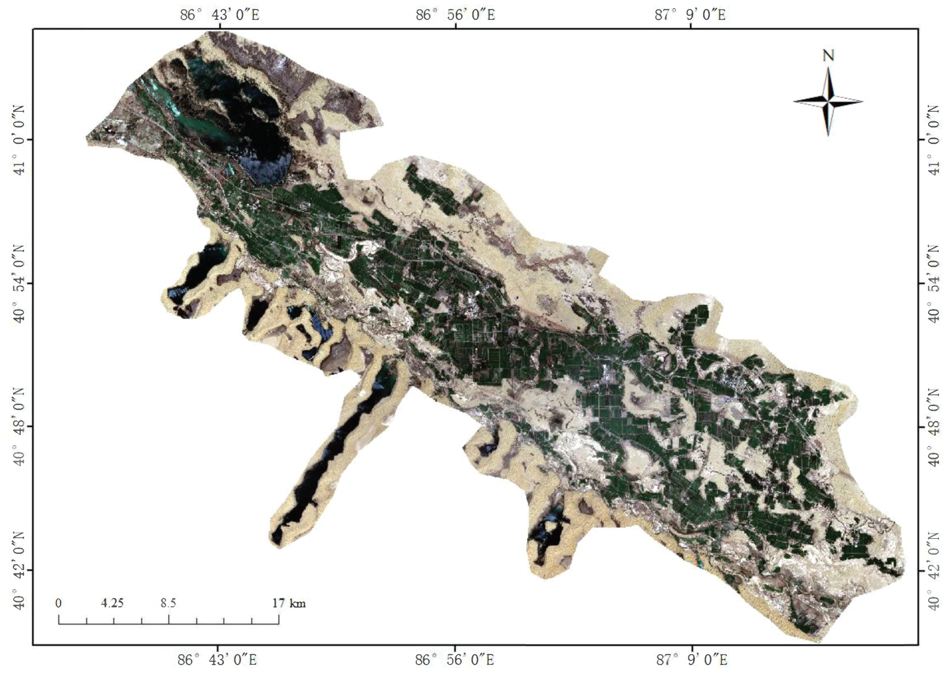
2.1. Study Area

We selected the 31st, 33rd Regiments and their surrounding areas of the Second Division of Xinjiang Production and Construction Corps, Yuli Comt, Bayinguoleng Mongolian Autonomous Prefecture, Xinjiang Uygur Autonomous Region, China. The study area range from 40 39 ′N to 41 4 ′N, and 86 35 ′E to 87 20 ′E. The location of the study area is shown in Figure 1. The study area of Yuli is 520 km from Urumqi City, 50 km south of Korla City, with a total area of 59,700 square kilometers. It includes seven townships, one town, nine communities, and 50 administrative villages. There are a total of five County level units, including three regiments of the second division (31st, 33rd, and 34th Regiments) and two state direct units (Qala Water Management Office, Tahe Bayinguoleng Authority Kongquehe downstream station). National Highway 218 crosses through the county and it is also one of the important transportation hubs in southern Xinjiang. The area is rich in types of ground features, including cultivated land, water, deserts mand roads. Therefore, it is suitable for remote sensing image classification study. Simultaneously, the study area is located between the Taklamakan Desert and the Kumtag Desert, and it is of great significance to understand the ecological situation of the study area by mastering the distribution of ground features.

2.2. Data and Samples

In the paper, we select Sentinel-2 data from June to August 2019, with a total of five scenes, specifically including three Sentinel-2A data scenes and two Sentinel-2B data scenes. Table 1 shows the data acquisition phase and other information.
The main land covers of the study area include desert, cotton land, roads, water, wetlands, uncultivated arable land, jujube trees, populus euphratica, buildings, woodland, pear trees, and other backgrounds, totaling 12 types of land covers. Figure 2 shows the main vegetation phenology information in the study area. Because the plants are in the summer growth period or flower bell period from June to August, the vegetation spectral and texture characteristics are more obvious, as shown in Figure 2. Additionally, when considering the quality of remote sensing images on the impact of remote sensing images classification, we select five scenes in this period. The Sentinel-2 image data used in the experiments are all from the European Space Agency, whose 1C level products are atmospheric apparent reflectance products that have undergone ortho correction and sub-pixel geometric fine correction, but no atmospheric correction. Accordingly, the plug-in Sen2cor released by ESA needs to be atmospherically corrected to obtain a 2A-grade product. Su et al. [50] proved that the plug-in has the highest accuracy by experiments. Because of different resolutions in 13 bands for images, we selected the visible light band with a ground resolution of 10m in Sentinel-2 as the data source, which is 2nd, 3rd, and 4th band (blue, green, and red), respectively.

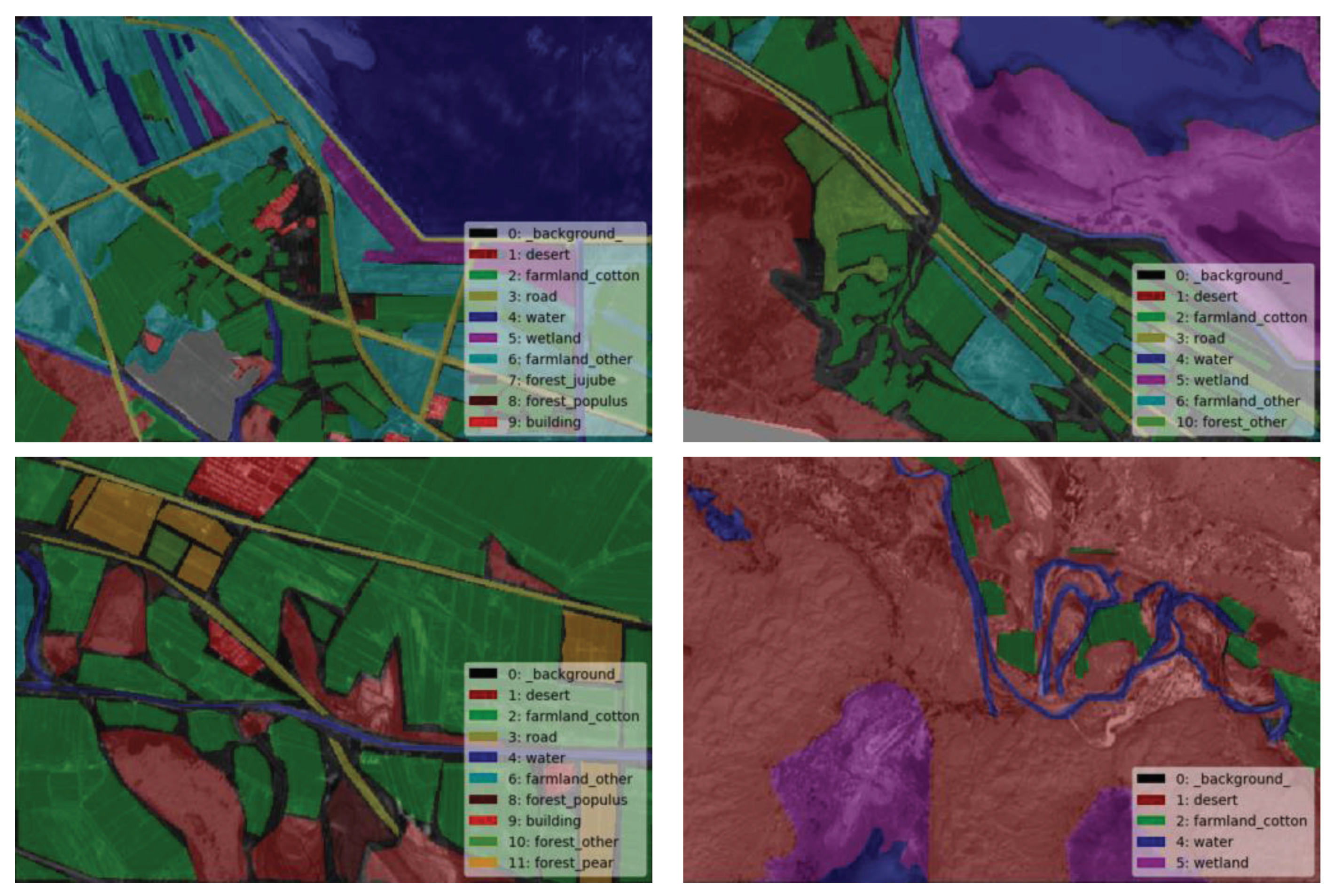
2.3. Dataset Preparation

The quality of the dataset is directly related to the accuracy of remote sensing image classification. The data annotations in this paper come from field investigations and they are combined with high-resolution Google Earth image visual interpretation. On 30 June 2019, the experimental team went to the study area for a detailed investigation, using high-precision GPS to record and take pictures of different land covers. Based on the location results, we labeled the Sentinel-2 data for 28 June 2019 after preprocessing while using the method mentioned above.
The data in this period are a mosaic of two scenes. Take study area as region of interest for image cutting, we get the image with size of 6338 × 4722 pixels. Subsequently, we cut it into subimages with the size of 500 × 334. The cut images are independent of each other without overlap, and the blank images are also removed by filtering. A total of 155 images are obtained. Next, label the image with Labelme software [51] to obtain the corresponding mark file. Because the selected image data gather from the same year with short time interval and without experiencing crop harvest or natural disasters and other great changes, vegetation is in the same period, water bodies, deserts, buildings, roads, etc. have not changed much too. The images do not need to be manually labeled repeatedly, and the shapes recorded in the first labeled file can be used to label the remote sensing images in the same area again [52,53]. Because remote sensing image classification is a multi-classification task, the category labels need to be fixed. We utilize the number from zero to eleven to mark the classes of land covers. These land covers are background, desert, cotton land, road, water, wetland, uncultivated arable land, jujube tree, populus euphratica, building, woodland, and pear tree, respectively.
After manual and repeated machine annotations, there generated 775 labeled images, and each one was 500 × 334 pixels in size. Figure 3 presents some labeling results.

2.4. Data Set Sample Distribution
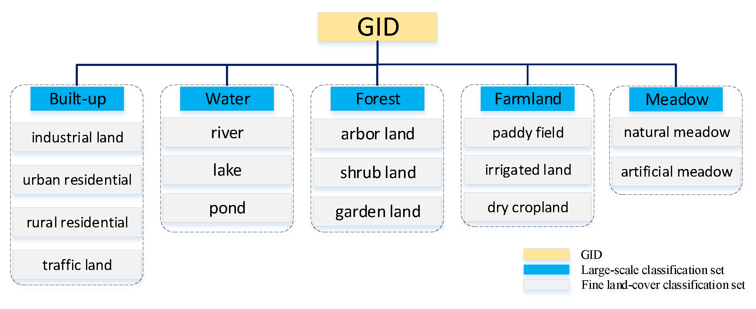
The annotated data set has a total of 775 pieces of Sentinel-2 satellite data, including five scenes from June to August, and the distribution of various land covers is shown in Table 2. Here shows the number of pixels and pictures for each kind of land covers. Where class frequency refers to the frequency of occurrence of this type of feature, and its formula is:
c l a s s f r e q u e n c y = p i i = 1 N P i
where p i represents the number of pixels occupied by the surface feature of class i, and P i represents the pixel size of the image of class i, which is 500 × 334 in this paper. N i is the number of images containing this class, and i = 1 N P i represents the sum of the total number of pixels of all images containing this ground feature class, which is, the number of pixels of images containing this class in the data set.
While w e i g h t in the table is designed to be assigned to a class in the loss function for median frequency balancing [29,54], and its value is the ratio of the median of class frequencies computed on the entire training set divided by the class frequency. The calculation formula is as follows:
w e i g h t i = m e d i a n ( c l a s s f r e q u e n c y ) c l a s s f r e q u e n c y i
For the land covers with a small proportion, its weight is greater than 1, while the weight is less than 1 for the land covers with a larger proportion. The smaller the proportion, the greater the weight. We measure the balance of the sample data based on the obtained weighting results. As can be seen from Table 2, land covers, such as desert and cotton land, are obviously in the dominant position of the big category. While the land covers such as pear trees have the smallest number of pixels and occupy a small number of pictures, resulting in a small class frequency, but not the largest weight. Because of the small number of pixels and large number of images, road features have a large class frequency and weight ratio, which need to be adjusted and paid attention to.

2.5. GID Dataset

We adopt Gaofen Image Dataset (GID) [55] as standard dataset to make comparison for our method verification. In the paper, partial GF-2 satellite images from the released GID dataset were utilized for preparing CNN model training samples, and the images only include red, blue, and green bands. GID consists of two main parts, namely large-scale classification and fine land-cover classification set. For the former, five representative land-use atecgories are annotated, built-up, farmland, forest, meadow, and water, respectively. These land-use categories were annotated, corresponding to five different colors: red, green, blue, cyan, yellow, and blue. In addition, areas not belonging to the above five categories and clutter regions are both labeled as background and are represented by black color. The fine land-cover classification set is composed of 15 sub-categories: paddy field, irrigated land, dry cropland, garden land, arbor forest, shrub land, natural meadow, artificial meadow, industrial land, urban residential, rural residential, traffic land, river, lake, and pond. Similarly, areas not belong to the above categories or unidentified manually are annotated as unknown areas, and are represented in black. We take the same strategy as [55] to cope with multispectral images, ignoring unknown regions, and only calculating the accuracy of deterministic regions. The two parts of GID constitute a hierarchical classification system, and Figure 4 shows the affiliation of them. In the paper, 50 GF-2 images form large-scale Classification set and 10 GF-2 images from fine land-cover classification set were extracted, and they were utilized for five-classification and ten-classification, respectively.

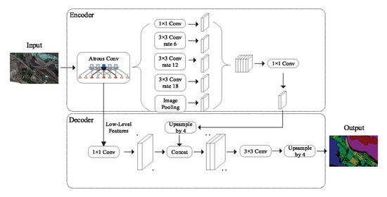
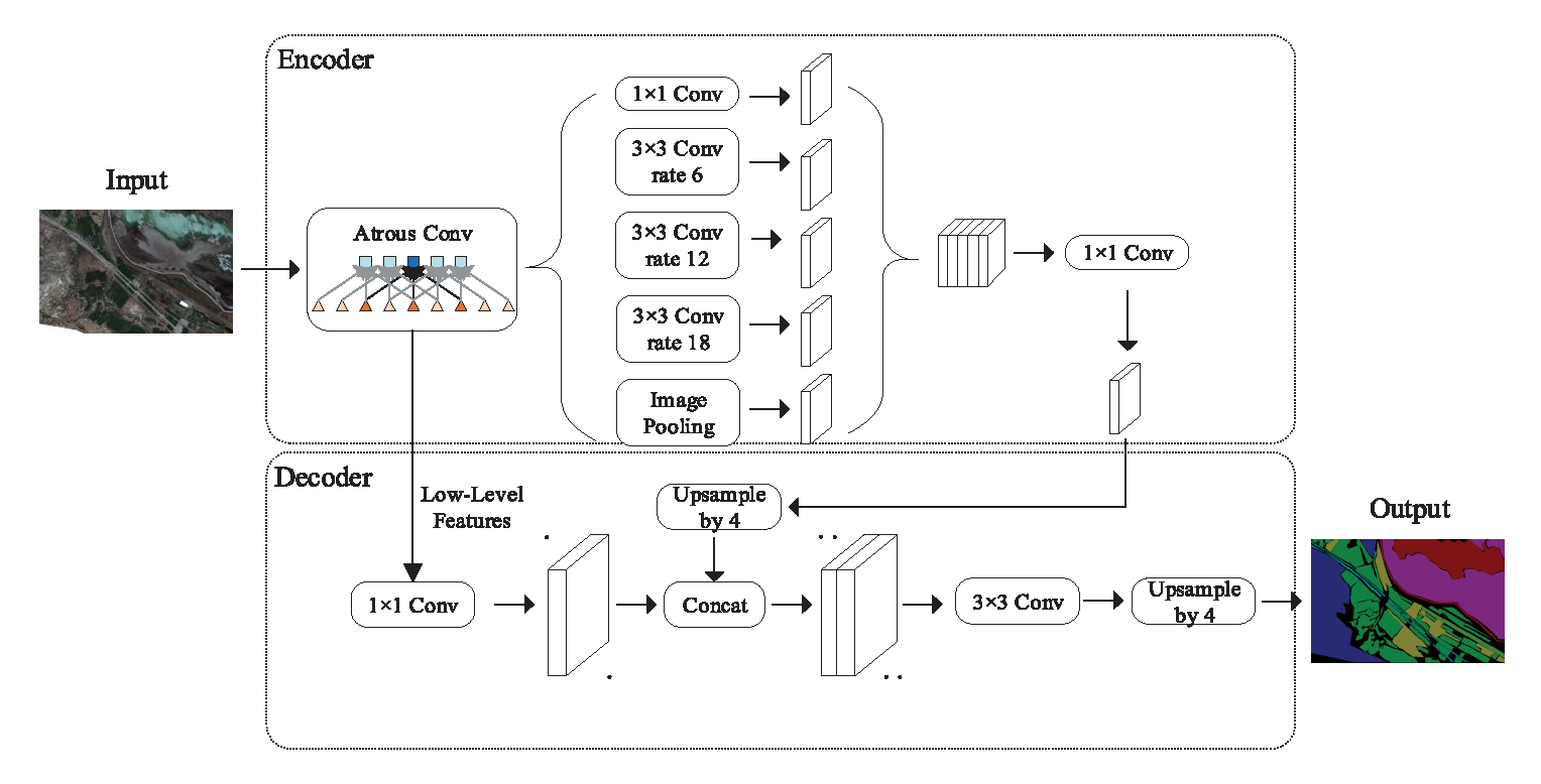
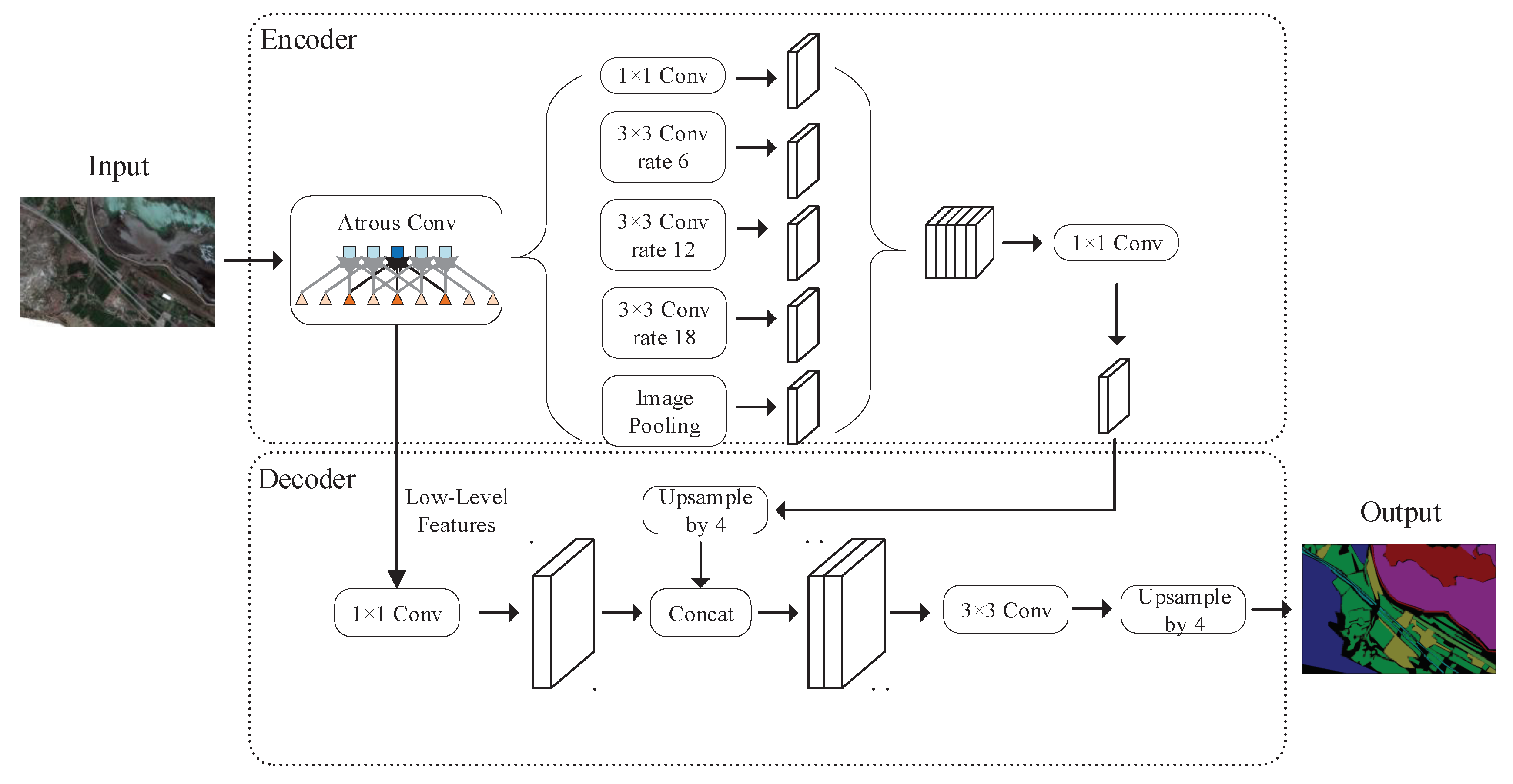
2.6. DeepLab v3+ Model

2.6.1. Overview

Figure 5 shows the architecture of DeepLab V3+, an image segmentation model based on deep full convolutional neural networks used in this paper. The network utilizes the Encode-Decoder structure with atrous convolution [30,31,56]. Among them, the Encoder part uses the DeepLab V3 network to encode multi-scale context information by with atrous convolution on multiple scales. The model takes the deep convolutional network Xception of atrous depthwise convolution [30,31] as the backbone network. Subsequently, multi-scale atrous convolution is used to encode multi-scale context information, while simple and effective decoder modules can be used to refine the classification results. The mathematical formula of atrous convolution is as follows:
y [ i ] = k x [ i + r k ] ω [ k ]
where y and ω represent the output feature map and the convolution filter, respectively. y [ i ] refers to the output of atrous convolution at each position i on the filter ω . The k is the filter’s kernel size, and x is the input feature map. The ratio of atrous convolution r is the sampling step of the input signal. The filter’s field-of-view can be modified by the modified value of r in order to obtain the output characteristics at any resolution. Therefore, the receptive field can be adjusted through atrous convolution to detect and segment large targets with high location accuracy. Besides, Multi-scale context information can be obtained by adjusting the parameter r.
The encoder part of the network is a process of extracting high-level semantic features, transforming low-dimensional features into abstract high-dimensional feature vectors. Therefore, DeepLab V3 + can extract feature vector with atrous convolution at any resolution. The output stride represents the ratio between the input image spatial resolution and the final output resolution before pooling or full connection layer, as shown in Equation (4). We set o u t p u t s t r i d e = 16 to perform image segmentation on remote sensing images.
o u t p u t s t r i d e = i n p u t i m a g e s p a t i a l r e s o l u t i o n f i n a l o u t p u t r e s o l u t i o n

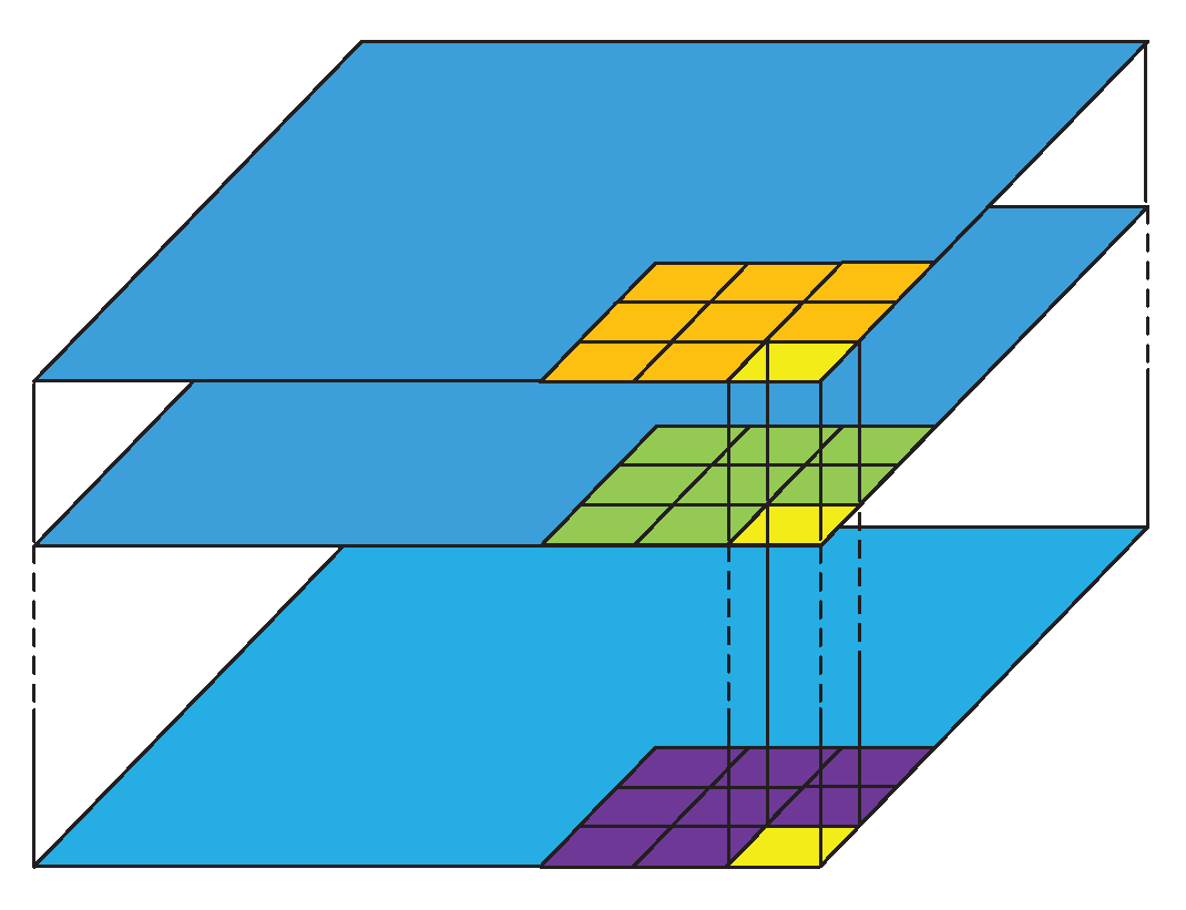
2.6.2. Atrous Spatial Pyramid Pooling with Depthwise Separable Convolution

In DeepLab V3+, the encoder takes DeepLab V3 network [31] as the base, simultaneously retaining atrous convolution and ASPP layer, and the backbone network adopts the method of Xception model, which can effectively improve the robustness and running speed of image segmentation. The method combines Atrous and Spatial Pyramid Pooling [57,58,59] in order to solve the multi-scale problem of image segmentation of objects by using four different rates of atrous convolution. ASPP includes a 1 × 1 convolution and three 3 × 3 atrous convolution with the sampling rate of rates = {6,12,18}, respectively. It also adopts image-level features, namely the features after global average optimization and convolution fusion, and the image pooling is performed, as shown in Figure 5. Because of in the process of image segmentation tasks with the existing convolutional neural network, down sampling will lead to information loss and the space invariance of convolutional neural network should be considered simultaneously.
In the paper, Depthwise separable convolution [60,61,62] is adopted to reduce the calculation cost and maintain model performance. Be different from conventional convolution operation, a convolution kernel of Depthwise convolution is responsible for one channel, and only one convolution kernel convolutes one channel. After depthwise convolution operation, the number of feature maps is the same as the number of channels in the input layer, so the pointwise convolution is needed in order to combine these feature maps to generate new feature maps, as shown in Figure 6. It is noteworthy that the operation of pointwise convolution is very similar to the conventional convolution operation. Its convolution kernel size is 1 × 1 × M, and M is the number of channels in the upper layer. Therefore, the convolution operation in this step will combine the feature map of the upper step in the depth direction to generate a new feature map.

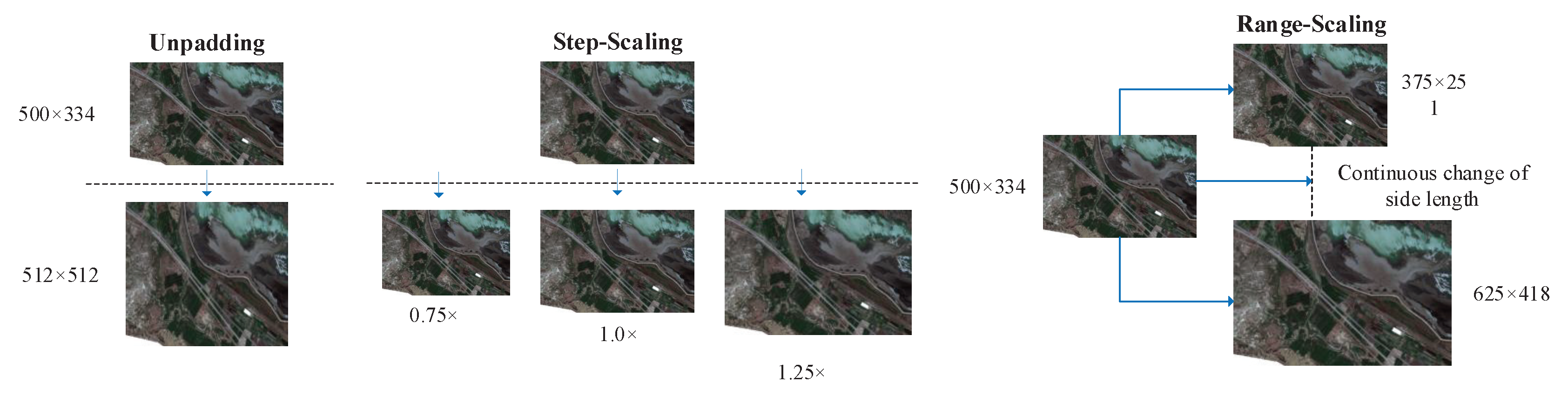
2.6.3. Data Augmentation

In deep learning algorithm, the quality of training depends on the quality of dataset. The spatial resolution of the Sentinel-2 data used in this paper is relatively high. The ground resolution of the band is up to 10 m with abundant features. Therefore, we can enhance the dataset obtained in Section 2.3 to prevent overfitting. The commonly used methods of data augmentation include image rollover, including left-right, up-down, and both together. Therefore, by flipping, there are four cases of the image, the original, left-right, up-down, and left-right-up-down, respectively. When satellites shoot land covers, they use a bird’s-eye view, and shooting at various positions is reasonable. There also exists other methods of data augmentation, such as Unpadding, Step-Scaling, and Range-Scaling, as shown in Figure 7. Specifically, unpadding is to use resize mode to scale the original image to 512 × 512 pixels. With step-scaling method, the original image is scaled up in a certain range by step size value. In this paper, we set scale parameter from 0.75 to 1.25, and the step size parameter is 0.25. If the range scaling method fixed the aspect ratio before training, then it will change in a certain range during training. The long edge needs to be aligned to a specified size during prediction. The specified size selected in this paper is 500, and the range of change is 400 to 600. The original dataset includes 775 pieces with 500 × 334 pixels each, and the number of flipped pieces was 775 × 4 pieces. The final number of flipped pieces was 775 × 4 × 2 × 3 × 2 after unpadding, step-scaling, and range-scaling, totally 37,200 pieces. The data set was divided into training set, verification set, and test set, and the ratio was 3:1:1.

2.6.4. Loss Function-Based Solution of Samples Imbalance

There exists many kinds of land covers in the study area, where the road covers little with small area. During training, imbalanced category distribution will be encountered. Softmax loss function treats each pixel equally during image segmentation, and generally adopted in multi classification tasks. The mathematical Equation (5) is as follows:
J s = 1 m i = 1 m j = 1 k l x i c j log e w J T x i l = 1 k e w l T x i
where w j R d refer the vector of weight w R d × k in column j. l { · } is the indicator function. As shown in Formula (6), x i c j means the label of the sample x i belongs to class j. Because the optimizer used in the model is SGD, the parameters can be optimized quickly in the gradient descent process.
l ( A ) = 1 A is true 0 A is false
It can be seen from the sample distribution in Section 2.4 that the road class features have a large class frequency and weight, which needs to be focused on. Due to the little cover proportion of road, samples are not balanced in multi-class tasks. While softmax loss evaluates the category of each pixel and finally evaluates the image with all pixels, and the training model will be dominated by the most mainstream category, reducing the network’s ability to extract roads. The combination of DICE and BCE loss can improve the stability of model training. Dice loss is defined as formula (7):
d i c e l o s s = 1 2 | Y P | | Y | + | P |
where | Y P | refers to the intersection of set Y and P. It can be seen from the formula that it measures the similarity of the two contours, and calculates the overlap between prediction and annotation to calculate the loss function. The combination of BCE loss function can improve the stability of model training. In this paper, the DICE and BCE loss functions are combined in order to improve detect accuracy for the surface features such as the road, while softmax loss function is still used for other surface features, improving the overall classification accuracy by comprehensively using these loss functions. For image segmentation of road, we compare the use of softmax and DICE-BCE loss function. The classification accuracy is as shown in Table 3. For road ground features, the DICE-BCE loss function can effectively improve its classification results and all three indicators are better than using only softmax loss function.

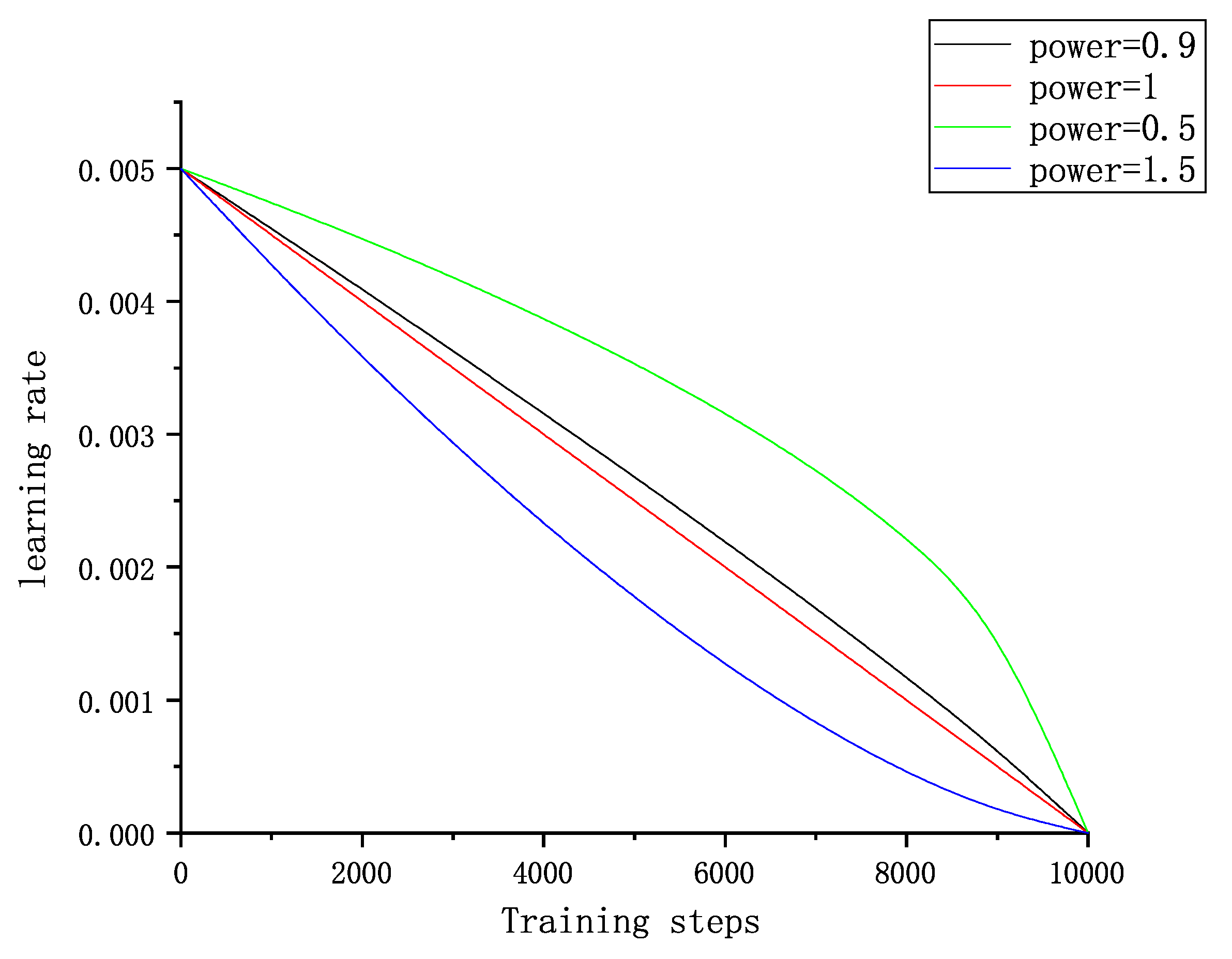
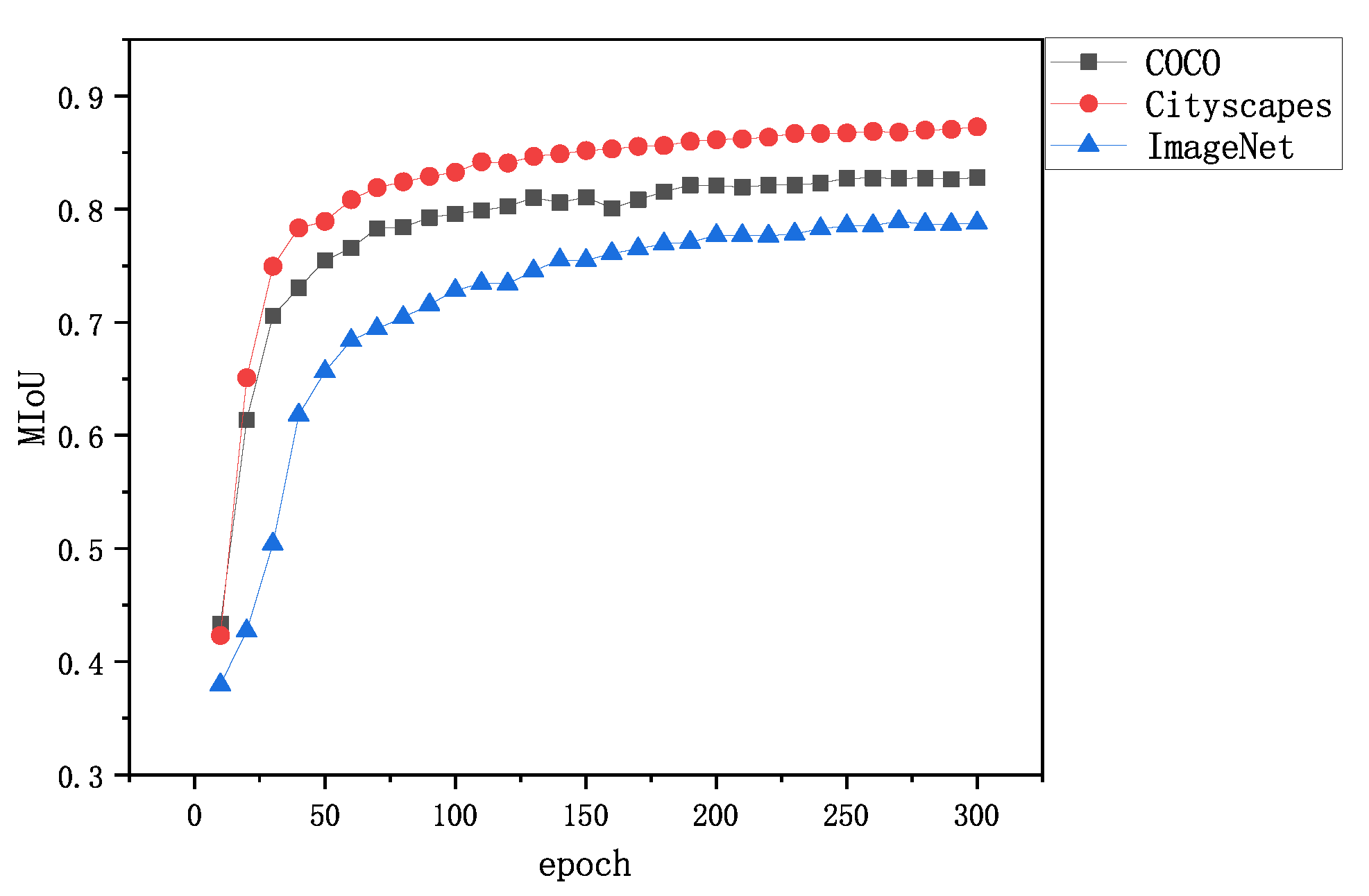
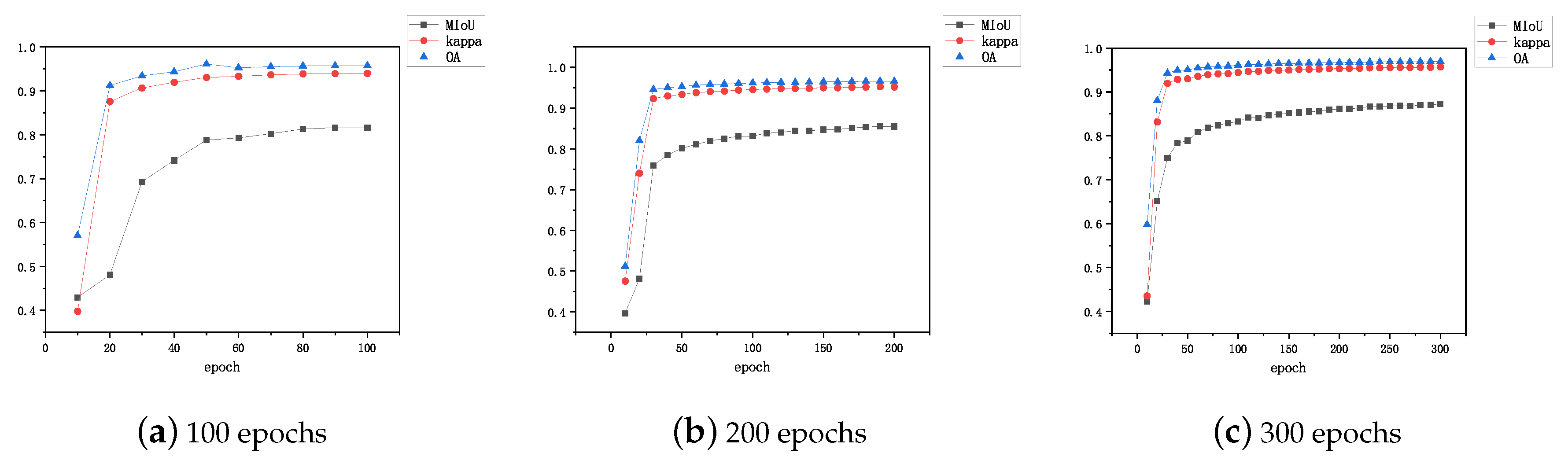
2.6.5. Model Training

For deep learning training, the storage and update of network weights take up huge amount of memory and resources. Hence, how to improve calculation efficiency is the crucial issue. In this paper, we adopt the network training method that is based on mixed precision [63] training to improve the training efficiency of the model. Mixed precision training, namely, based on the complexity and accuracy requirements of data calculation, single-precision format (FP32) and IEEE half-precision format (FP16) are flexibly chosen in order to carry network weights, instead of conventional completely using FP32. The difference between the two precision modes, is shown in Table 4. Specifically, the model parameters are stored in FP32, and FP16 is chosen for the forward calculation of the network. Due to back-propagation involving weight update, FP32 was used to prevent weight parameters from missing because of the lack of accuracy. Simultaneously, the loss scaling factor is introduced into training to avoid overflow and underflow.

3. Results

3.1. Experimental Environment and Model Training

The experiments were performed on an Ubuntu 16.04LTS 64-bit system, while using NVIDIA Titan XP for graphics acceleration. The model uses the ploy strategy to attenuate the learning rate, and the formula is as follows:
L R = I n i t i a l L R 1 i t e r m a x i t e r p o w e r
The initial learning rate I n i t i a l L R is 0.005, the learning rate decay strategy decline index p o w e r is 0.9, and the m a x i t e r is the maximum training step size. i t e r refers to current training step length. Figure 8 shows different decay curves. When p o w e r = 1 , the learning rate decay curve is a straight line, when p o w e r > 1 , the learning rate decay curve turns to concave inside and when p o w e r < 1 , the learning rate decay curve turns to convex outside. In this paper, we use random gradient descent algorithm with p o w e r = 0.9 for parameter optimization. The whole training process includes 100 batches with a total of 12.900 steps with several kinds of loss functions.

3.2. Evaluating Indicator

We use classification accuracy (CA), overall accuracy (OA), intersection over Union (IoU), mean intersection over Union (MIoU), and kappa coefficients as evaluation indexes in order to evaluate the segmentation accuracy of the model in remote sensing image reasonably and objectively. The larger the index value, the better the model effect.
(1) Classification Accuracy and Overall Classification Accuracy
Classification accuracy (CA), which can directly express the classification accuracy of a certain class of pixels, is expressed by the ratio of the correct number of pixels in this class to the total number of all pixels in this class. The formula is as follows:
CA = p i i j = 0 k p i j
where we assume there exists k + 1 classes (including k target classes and 1 background class). In this paper, k is 11. p i i represents the number of pixel i correctly predicted as i and p i j represents the number of pixel i predicted as j.
Overall classification accuracy (OA) can express the overall classification accuracy of pixel points, and calculate the ratio of pixel points with correct overall classification and the total number of all pixel points. The formula is as follows:
OA = i = 0 k p i i i = 0 k j = 0 k p i j
(2) Intersection over Union and Mean Intersection over Union
Intersection over Union (IoU) is a standard metric of the image segmentation model. It calculates the ratio of the intersection and union of the ith type true value pixel set and predicted value pixel set. It is defined, as follows:
IoU = p i i j = 0 k p i j + j = 0 k p i j p i i
The Mean Intersection over Union (MIoU) is to calculate the intersection ratio of each class and calculating the average of all classes. This index can better reflect the accuracy and completeness of model segmentation in different terrain type areas in the experiment, as defined below:
MIOU = 1 k + 1 i = 0 k p i i j = 0 k p i j + j = 0 k p i j p i i
(3) Kappa coefficient
The Kappa coefficient is an index for consistency check. It can measure the effect of classification or segmentation. The value range is [−1,1], the closer it is to 1, the better the classification or segmentation effect, the definition is as follows:
kappa = p o p e 1 p e
where, p o is the overall classification accuracy, assuming that the real number of samples of each class is a 1 , a 2 , …, a ( k + 1 ) , and the predicted number of samples of each class is b 1 , b 2 , …, b ( k + 1 ) , the total number of samples is n, then:
p e = a 1 × b 1 + a 2 × b 2 + + a ( k + 1 ) × b ( k + 1 ) n × n

3.3. Training Protocol

Pre-train: due to limited remote sensing image dataset, public datasets were considered for model pre-training, namely ImageNet [64], COCO [65] and Cityscape [66]. Then remote sensing image training dataset was feed into the initialized model, and MIoU results were shown as Figure 9. It can be seen that model pre-trained by ImageNet performed worst. Model pre-trained by COCO and Cityscape show approximate MIoU value at first, while cityscape-based model accelerate the convergence speed gradually and finally achieved better performance. Therefore, the cityscape dataset was selected for model pre-training.
Norm Type: as the number of network layers increase, the distribution of weight will gradually shift with the training of the network, causing declining feature representing ability and slow convergence speed. To address the problem, we selected Batch Normalization (BN) [67] and Group Normalization (GN) [68] for model training, and made verification comparison on validation set with MIoU. The BN-based method outperforms with faster convergence speed and high MIoU value, as shown in Figure 10. That is because GN-based method cannot handle loss value with type of NaN. Consequently, we select BN as the normalization-based method.
The number of training epochs: We vary the number of training epochs as [100, 200, 300]. Figure 11 shows the experimental results. We can see that, as the number of epochs increases, the performance of the model is gradually improved. Subsequently, the model starts to converge form the 50th epoch, and the performance becomes stabilized when the epoch reaches the 200th epoch. In order to make model fully trained, we set the number of epoch to 300.

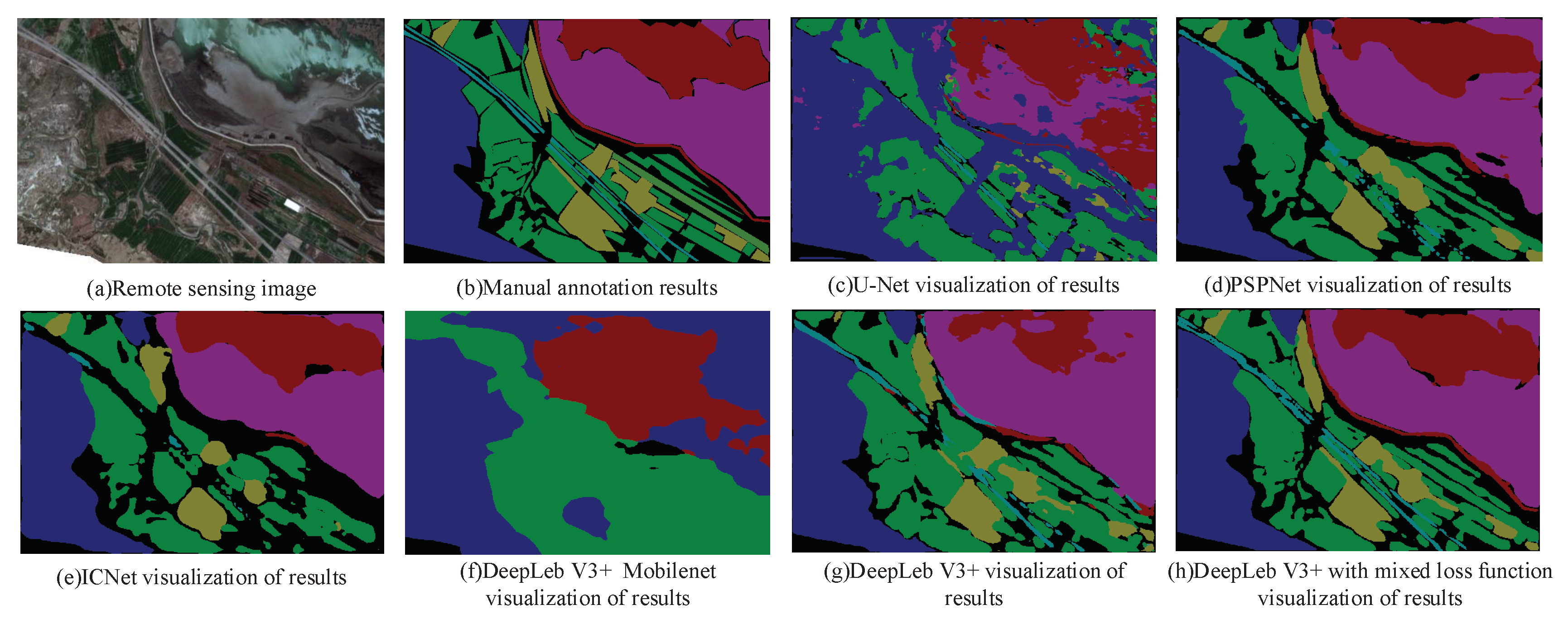
3.4. Experiment Result Analysis

In the paper, we compared our improved loss function-based method with four mainstream segmentation network: U-Net, PSPNet, ICNet, and DeepLab V3+. Table 5 shows the experimental results on the satellite image dataset.
In order to evaluate the impact of each model on the extraction accuracy of various land covers quantitatively and accurately, we utilize the test set to evaluate the accuracy of different models with indicators, such as: OA, MIoU, Kappa coefficient, CA and IoU. Table 5 shows that the U-Net model utilizes the COCO data set for pre-training initialization, with an overall accuracy of 86.16%. PSPNet and ICNet model utilizes the Cityscapes data set for pre-training initialization, with an overall accuracy of 95.88% and 93.97%, respectively. In Deeplab V3+ mobilenet model, we take mobilenet V2 as the backbone network. Subsequently, we utilize COCO dataset for pre-training initialization, and the overall accuracy reaches 81.79%. Simultaneously, we take Xception as the backbone network, initializing the model with Cityscapes dataset and the overall accuracy reaches 95.77%. In this paper, we select a loss-function hybrid model based on DeepLab V3+. The backbone network of model is Xception. The model utilizes Cityscapes dataset for pre-training. As a result, the overall accsuracy reaches 97.97%, which outperforms other models, especially on the road detection. This is because the roads belong to small class samples and softmax loss function always treats any pixels equally. In case of unbalanced samples, it will lead to classification biased towards large types of features if only using the softmax loss function. In this paper, the method is to deal with the road with the combination of DICE and BCE loss function, which greatly improves the segmentation accuracy of small class samples and overall classification accuracy.
The Kappa coefficients are 0.8000, 0.9415, 0.9144, 0.7367, 0.9401, and 0.9587, respectively. It can be seen that the model based on DeepLab V3+ model with mixed use of loss function has the highest Kappa coefficient with the best segmentation effect. The U-Net model has a poor classification result due to the simple network structure and the lack of multi-scale context information, which results in misclassification because of “salt and pepper noise”. Therefore, the Kappa coefficient is relatively low. ICNet obtains semantic information through low-resolution branches, and takes medium-resolution and high-resolution branches for recovery and refinement of rough predictions. However, because of low input resolution and small amount of calculation, the Kappa coefficient obtained is not optimal. Because PSPNet can combine multi-scale context information, and 50-layer ResNet, as the backbone network, also has a strong expression ability, the boundary segmentation effect is better. DeepLab V3+ has poor segmentation ability in the case of insufficient trunk network expression ability, such as MobileNet, but, in the case of strong trunk network capability, such as Xception, it has strong segmentation ability. Because PSPNet does not combine the low-level rich spatial information for decoding, its segmentation boundaries are relatively rough. While DeepLab V3+ architecture combines multi-scale context information, the segmentation boundaries are refined by the Encoder-Decoder structure. The performance is shown as Figure 12. In the figure, (a) is the original remote sensing image, (b) is the ground truth of the manually labeled result, and (c) to (h) are the visual results of u-net, PSPNet, ICNet, DeepLabv3+ Mobilenet, DeepLeb V3+, and DeepLeb V3+ with mixed loss function, respectively. It is not difficult to see from the Figure 12 that U-Net has a large area of “salt and pepper noise”, which seriously affects the classification effect. While the classification performance of DeepLeb V3+ Mobilenet is fuzzy, and the result is also unsatisfactory. Although the results of PSPNet and ICNet are generally correct, the boundary of ground object classification is not clear with fuzzy edge contour. The boundary of the features divided by DeeLab V3+ network is clear and complete, and the classification is accurate.
We also conducted experiments on GID dataset in order to test the effectiveness of this model. Accordingly, we compared our model with object-based classification methods and other general segmentation network, and the experimental result is shown in Table 6. Our method outperforms other algorithms, indicating the effectiveness on public high resolution remote sensing image dataset, as shown in Table 6. Although the acquisition location and time are diverse, the objects belong to the same class have similar spectral response in the images that were captured by the same sensor (i.e., GF-2 satellite). It can be seen that our model achieved the highest Kappa and OA of 0.6355 and 74.98% on five classes, and of 0.5979 and 69.16% on 15 classes, showing the strong transferability and effectiveness of the model.

4. Discussion

As mentioned above in Section 2.4, desert, cotton land, water, wetland, and background, as the large classes, are of the great sample size. Therefore, various models get well trained, and the classification effect is relatively good. Uncultivated arable land, jujube trees, populus euphratica, building, woodland and pear trees, etc., as the classes occupy a relatively small sample size, so various models have poor training effects on these small classes. It is obvious in DeepLabv3+ Mobilenet that the accuracy of these categories is seriously affected due to the lack of backbone network expression ability. In addition, the overlap between the classified markers and ground truth can be understood by observing the IoU values. In U-Net, the classification effect of these categories is only slightly improved, owing to the thin number of network layers, but the low IoU value is still unsatisfactory. As a contrast, PSPNet, ICNet, and DeepLab V3+ extract rich underlying semantic features by using multi-scale context, which greatly improves the recognition accuracy of these categories. PSPNet and DeepLab V3+ have similar classification effects, with a classification accuracy of over 80%, while ICNet is slightly inferior, with over 70%. However, their IoU value is relatively low, only over 70%, indicating that the classified labels and ground truth do not coincide well. For the road ground features, as the small class with high weight, the training effect of the above models is general with poor classification accuracy, and the IoU value is also low.
In the paper, the model proposed based on the DeepLab V3 + network using a mixed loss function has better effects on road edges and higher overall accuracy. The accuracy reached 97.47% and the IoU was 76.02%, both of which outperform other models. When compared to Figure 12g trained only by DeepLab V3 + model, the road edge is more complete with a better classification effect and fewer error marks than the rest of the visual structure in Figure 12h. Simultaneously, the average intersection ratio is also higher, reaching 87.74%. By the one-scene labeling, multi-scene image data can be used to build a richer dataset. The dataset obtained by the data augmentation method is different from the previous methods, which enhances the generality of the model ability to make classification better.
The experimental results demonstrate that the proposed model outperforms other deep learning models. In this paper, the method helps to solve the samples imbalance problem and improve classification accuracy for small class samples by mixed use of loss function. It improves the generalization ability of the model and the classification effect of the model by image marking methods and enhancement methods. As a whole, the overall accuracy, average occurring, and Kappa coefficient have been improved. The effectiveness of the model is reflected in three aspects: (1) the DeepLab V3+ model extracts high-level semantic features from multi-scale context information, the encoder-decoder structure combines low-level spatial information and high-level semantic information to recover ground object boundaries more effectively. (2) Mixed use of DICE and BCE loss function is to deal with small class samples, which helps to improve classification accuracy and achieve better segmentation performance. (3) The data are enhanced by one-phase annotation and multi-phase remote sensing image data, saving the work of visual interpretation. We verify the effectiveness of our model when comparing with traditional machine learning methods and mainstream segmentation networks on GID dataset.

5. Conclusions

The problem of class imbalance limits the classification accuracy of the model for small-scale objects, and then affects the overall effect of image segmentation. In this paper, when considering high-resolution remote sensing image space has the characteristics of high resolution, low spectral resolution, large-scale size with complex land covers, and unclear image prospects resulting from large intra-category differences or small inter-category differences. In this paper, DeepLab V3+, an image segmentation algorithm that is based on the full convolutional neural network, is selected and improved and Sentinel-2 data of remote sensing image around Yuli County, Bayingolin Mongol Autonomous Prefecture, Xinjiang Uygur Autonomous Region are used as the data source. Additionally, a high-resolution remote sensing image data set of the reaserch area was sorted out. The data set of the multi-date labeled image was obtained by labeling the one-date image, and the data set of the study area was obtained for model training through data augmentation. And the distribution of samples within the data set is analyzed. The experimental results demonstrate that the proposed model can be effectively used for image segmentation of the remote sensing image. When compared with U-Net, PSPNet, ICNet, and the proposed method help to improve classification for small class samples. Subsequently, the overall classification accuracy and average intersection ratio both get improved. The overall accuracy reaches 97.97% and the average intersection ratio reaches 87.74%. We verify the effectiveness of the proposed model on the GID dataset.
We will consider such two improvements in our future work. For one, as well known there are not only spectral resolution scale, spatial resolution scale, but also temporal resolution scale in the classification task of remote sensing imagery, and we just make use of spatial resolution and spectral resolution in our previous work. Our further work is to consider how to add the temporal resolution to the network in order to improve the classification accuracy. For another, the model adopted in the paper is relatively complex, and the calculation of parameters is large. When facing a large number of remote sensing image data, it also needs to consider how to improve the efficiency of the algorithm and realize the fast remote sensing image classification while maintaining the certain performance of the algorithm. Although it has accelerated the operation by deep separable convolution and mixed precision training methods in the paper, we still need to consider enhancing the classification performance of the model in the future.

Author Contributions

Conceptualization, X.Z. and C.W.; methodology, Y.R. and C.W.; software, Y.R. and C.W.; validation, Y.R.; formal analysis, Y.R. and Y.M.; data curation, Y.R. and Q.Y.; writing—original draft preparation, Y.R.; writing—review and editing, H.L. and Q.Q.; supervision, C.W. and Q.Q. All authors have read and agreed to the published version of the manuscript.

Funding

This research was funded by National Key Research and Development Program of China (2017YFB0504203); National Natural Science Foundation of China (41461088); Xinjiang Production and Construction Corps Science and Technology Program (2016AB001, 2017DB005).

Conflicts of Interest

The authors declare no conflict of interest.

References

  1. Zhang, C.; Chen, Y.; Yang, X.; Gao, S.; Li, F.; Kong, A.; Zu, D.; Sun, L. Improved remote sensing image classification based on multi-scale feature fusion. Remote Sens. 2020, 12, 213. [Google Scholar] [CrossRef] [Green Version]
  2. Hu, F.; Xia, G.S.; Hu, J.; Zhang, L. Transferring deep convolutional neural networks for the scene classification of high-resolution remote sensing imagery. Remote Sens. 2015, 7, 14680–14707. [Google Scholar] [CrossRef] [Green Version]
  3. Hossain, M.D.; Chen, D. Segmentation for Object-Based Image Analysis (OBIA): A review of algorithms and challenges from remote sensing perspective. ISPRS J. Photogramm. Remote Sens. 2019, 150, 115–134. [Google Scholar] [CrossRef]
  4. Wang, S.; Chen, W.; Xie, S.M.; Azzari, G.; Lobell, D.B. Weakly supervised deep learning for segmentation of remote sensing imagery. Remote Sens. 2020, 12, 207. [Google Scholar] [CrossRef] [Green Version]
  5. Kaiser, P.; Wegner, J.D.; Lucchi, A.; Jaggi, M.; Hofmann, T.; Schindler, K. Learning aerial image segmentation from online maps. IEEE Trans. Geosci. Remote Sens. 2017, 55, 6054–6068. [Google Scholar] [CrossRef]
  6. Du, S.; Du, S.; Liu, B.; Zhang, X. Context-Enabled Extraction of Large-Scale Urban Functional Zones from Very-High-Resolution Images: A Multiscale Segmentation Approach. Remote Sens. 2019, 11, 1902. [Google Scholar] [CrossRef] [Green Version]
  7. Kavzoglu, T.; Erdemir, M.Y.; Tonbul, H. Classification of semiurban landscapes from very high-resolution satellite images using a regionalized multiscale segmentation approach. J. Appl. Remote Sens. 2017, 11, 035016. [Google Scholar] [CrossRef]
  8. Na, X.; Zhang, S.; Zhang, H.; Li, X.; Yu, H.; Liu, C. Integrating TM and ancillary geographical data with classification trees for land cover classification of marsh area. Chin. Geogr. Sci. 2009, 19, 177–185. [Google Scholar] [CrossRef]
  9. Lv, X.; Ming, D.; Lu, T.; Zhou, K.; Wang, M.; Bao, H. A new method for region-based majority voting CNNs for very high resolution image classification. Remote Sens. 2018, 10, 1946. [Google Scholar] [CrossRef] [Green Version]
  10. Yang, X.; Zhao, S.; Qin, X.; Zhao, N.; Liang, L. Mapping of urban surface water bodies from Sentinel-2 MSI imagery at 10 m resolution via NDWI-based image sharpening. Remote Sens. 2017, 9, 596. [Google Scholar] [CrossRef] [Green Version]
  11. Jia, K.; Liang, S.; Wei, X.; Yao, Y.; Su, Y.; Jiang, B.; Wang, X. Land cover classification of Landsat data with phenological features extracted from time series MODIS NDVI data. Remote Sens. 2014, 6, 11518–11532. [Google Scholar] [CrossRef] [Green Version]
  12. Li, K.; Chen, Y. A Genetic Algorithm-based urban cluster automatic threshold method by combining VIIRS DNB, NDVI, and NDBI to monitor urbanization. Remote Sens. 2018, 10, 277. [Google Scholar] [CrossRef] [Green Version]
  13. Han, J.; Zhang, D.; Cheng, G.; Guo, L.; Ren, J. Object detection in optical remote sensing images based on weakly supervised learning and high-level feature learning. IEEE Trans. Geosci. Remote Sens. 2014, 53, 3325–3337. [Google Scholar] [CrossRef] [Green Version]
  14. Kavzoglu, T.; Tonbul, H. An experimental comparison of multi-resolution segmentation, SLIC and K-means clustering for object-based classification of VHR imagery. Int. J. Remote Sens. 2018, 39, 6020–6036. [Google Scholar] [CrossRef]
  15. Molada-Tebar, A.; Marqués-Mateu, Á.; Lerma, J.L.; Westland, S. Dominant Color Extraction with K-Means for Camera Characterization in Cultural Heritage Documentation. Remote Sens. 2020, 12, 520. [Google Scholar] [CrossRef] [Green Version]
  16. Hengst, A.M.; Armstrong, W., Jr. Automated Delineation of Proglacial Lakes At Large Scale Utilizing Google Earth Engine Maximum-Likelihood Land Cover Classification. AGUFM 2019, 2019, C31A–1481. [Google Scholar]
  17. Wang, K.; Cheng, L.; Yong, B. Spectral-Similarity-Based Kernel of SVM for Hyperspectral Image Classification. Remote Sens. 2020, 12, 2154. [Google Scholar] [CrossRef]
  18. Guo, Y.; Jia, X.; Paull, D. Effective sequential classifier training for SVM-based multitemporal remote sensing image classification. IEEE Trans. Image Process. 2018, 27, 3036–3048. [Google Scholar]
  19. Bazi, Y.; Melgani, F. Convolutional SVM networks for object detection in UAV imagery. IEEE Trans. Geosci. Remote Sens. 2018, 56, 3107–3118. [Google Scholar] [CrossRef]
  20. Zhu, X.; Li, N.; Pan, Y. Optimization performance comparison of three different group intelligence algorithms on a SVM for hyperspectral imagery classification. Remote Sens. 2019, 11, 734. [Google Scholar] [CrossRef] [Green Version]
  21. Paoletti, M.E.; Haut, J.M.; Tao, X.; Miguel, J.P.; Plaza, A. A new GPU implementation of support vector machines for fast hyperspectral image classification. Remote Sens. 2020, 12, 1257. [Google Scholar] [CrossRef] [Green Version]
  22. Yang, C.; Wu, G.; Ding, K.; Shi, T.; Li, Q.; Wang, J. Improving land use/land cover classification by integrating pixel unmixing and decision tree methods. Remote Sens. 2017, 9, 1222. [Google Scholar] [CrossRef] [Green Version]
  23. Belgiu, M.; Drăguţ, L. Random forest in remote sensing: A review of applications and future directions. ISPRS J. Photogramm. Remote Sens. 2016, 114, 24–31. [Google Scholar] [CrossRef]
  24. Zafari, A.; Zurita-Milla, R.; Izquierdo-Verdiguier, E. Evaluating the performance of a random forest kernel for land cover classification. Remote Sens. 2019, 11, 575. [Google Scholar] [CrossRef] [Green Version]
  25. LeCun, Y.; Bengio, Y.; Hinton, G. Deep learning. Nature 2015, 521, 436–444. [Google Scholar] [CrossRef] [PubMed]
  26. Long, J.; Shelhamer, E.; Darrell, T. Fully convolutional networks for semantic segmentation. In Proceedings of the IEEE Conference on Computer Vision and Pattern Recognition, Boston, MA, USA, 7–12 June 2015; pp. 3431–3440. [Google Scholar]
  27. Ronneberger, O.; Fischer, P.; Brox, T. U-net: Convolutional networks for biomedical image segmentation. In Proceedings of the International Conference on Medical Image Computing and Computer-Assisted Intervention, Munich, Germany, 5–9 October 2015; pp. 234–241. [Google Scholar]
  28. Zhao, H.; Shi, J.; Qi, X.; Wang, X.; Jia, J. Pyramid scene parsing network. In Proceedings of the IEEE Conference on Computer Vision and Pattern Recognition, Honolulu, HI, USA, 21–26 June 2017; pp. 2881–2890. [Google Scholar]
  29. Badrinarayanan, V.; Kendall, A.; Cipolla, R. Segnet: A deep convolutional encoder-decoder architecture for image segmentation. IEEE Trans. Pattern Anal. Mach. Intell. 2017, 39, 2481–2495. [Google Scholar] [CrossRef] [PubMed]
  30. Chen, L.C.; Papandreou, G.; Kokkinos, I.; Murphy, K.; Yuille, A.L. Deeplab: Semantic image segmentation with deep convolutional nets, atrous convolution, and fully connected crfs. IEEE Trans. Pattern Anal. Mach. Intell. 2017, 40, 834–848. [Google Scholar] [CrossRef]
  31. Chen, L.C.; Papandreou, G.; Schroff, F.; Adam, H. Rethinking atrous convolution for semantic image segmentation. arXiv 2017, arXiv:1706.05587. [Google Scholar]
  32. Chen, L.C.; Zhu, Y.; Papandreou, G.; Schroff, F.; Adam, H. Encoder-decoder with atrous separable convolution for semantic image segmentation. In Proceedings of the European Conference on Computer Vision (ECCV), Munich, Germany, 8–14 September 2018; pp. 801–818. [Google Scholar]
  33. Zhao, H.; Qi, X.; Shen, X.; Shi, J.; Jia, J. Icnet for real-time semantic segmentation on high-resolution images. In Proceedings of the European Conference on Computer Vision (ECCV), Munich, Germany, 8–14 September 2018; pp. 405–420. [Google Scholar]
  34. Zhao, W.; Du, S. Learning multiscale and deep representations for classifying remotely sensed imagery. ISPRS J. Photogramm. Remote Sens. 2016, 113, 155–165. [Google Scholar] [CrossRef]
  35. Mnih, V. Machine Learning for Aerial Image Labeling. Ph.D. Thesis, University of Toronto, Toronto, ON, Canada, 2013. [Google Scholar]
  36. Wang, E.; Qi, K.; Li, X.; Peng, L. Semantic Segmentation of Remote Sensing Image Based on Neural Network. Acta Opt. Sin. 2019, 39, 1210001. [Google Scholar] [CrossRef]
  37. Wei, Y.; Wang, Z.; Xu, M. Road structure refined CNN for road extraction in aerial image. IEEE Geosci. Remote Sens. Lett. 2017, 14, 709–713. [Google Scholar] [CrossRef]
  38. Kemker, R.; Salvaggio, C.; Kanan, C. Algorithms for semantic segmentation of multispectral remote sensing imagery using deep learning. ISPRS J. Photogramm. Remote Sens. 2018, 145, 60–77. [Google Scholar] [CrossRef] [Green Version]
  39. He, H.; Wang, S.; Yang, D.; Shuyang, W.; Liu, X. An road extraction method for remote sensing image based on Encoder-Decoder network. Acta Geod. Cartogr. Sin. 2019, 48, 330. [Google Scholar]
  40. Zhang, H.; Wang, B.; Han, W.; Yang, J.; Pu, P.; Wei, J. Extraction of Irrigation Networks in Irrigation Area of UAV Orthophotos Based on Fully Convolutional Networks. Trans. Chin. Soc. Agric. Mach. 2019, 27. [Google Scholar]
  41. Wu, Z.; Gao, Y.; Li, L.; Xue, J. Fully Convolutional Network Method of Semantic Segmentation of Class Imbalance Remote Sensing Images. Acta Opt. Sin. 2019, 39, 0428004. [Google Scholar]
  42. Zhu, T.; Dong, F.; Gong, H. Remote Sensing Building Detection Based on Binarized Semantic Segmentation. Acta Opt. Sin. 2019, 39, 1228002. [Google Scholar]
  43. Yang, J.; Zhou, Z.; Du, Z.; Xu, Q.; Yin, H.; Liu, R. Rural construction land extraction from high spatial resolution remote sensing image based on SegNet semantic segmentation model. Trans. Chin. Soc. Agric. Eng. 2019, 35, 251–258. [Google Scholar]
  44. Li, K.; Wan, G.; Cheng, G.; Meng, L.; Han, J. Object detection in optical remote sensing images: A survey and a new benchmark. ISPRS J. Photogramm. Remote Sens. 2020, 159, 296–307. [Google Scholar] [CrossRef]
  45. Paoletti, M.; Haut, J.; Plaza, J.; Plaza, A. Deep learning classifiers for hyperspectral imaging: A review. ISPRS J. Photogramm. Remote Sens. 2019, 158, 279–317. [Google Scholar] [CrossRef]
  46. Garcia-Garcia, A.; Orts-Escolano, S.; Oprea, S.; Villena-Martinez, V.; Martinez-Gonzalez, P.; Garcia-Rodriguez, J. A survey on deep learning techniques for image and video semantic segmentation. Appl. Soft Comput. 2018, 70, 41–65. [Google Scholar] [CrossRef]
  47. Niu, Z.; Liu, W.; Zhao, J.; Jiang, G. Deeplab-based spatial feature extraction for hyperspectral image classification. IEEE Geosci. Remote Sens. Lett. 2018, 16, 251–255. [Google Scholar] [CrossRef]
  48. Wasikowski, M.; Chen, X.W. Combating the small sample class imbalance problem using feature selection. IEEE Trans. Knowl. Data Eng. 2009, 22, 1388–1400. [Google Scholar] [CrossRef]
  49. Chawla, N.V.; Japkowicz, N.; Kotcz, A. Special issue on learning from imbalanced data sets. ACM SIGKDD Explor. Newsl. 2004, 6, 1–6. [Google Scholar] [CrossRef]
  50. Su, W.; Zhang, M.; Jiang, K.; Zhu, D.; Huang, J.; Wang, P. Atmospheric Correction Method for Sentinel-2 Satellite Imagery. Acta Opt. Sin. 2018, 38, 0128001. [Google Scholar] [CrossRef]
  51. GitHub—Wkentaro/Labelme: Image Polygonal Annotation with Python (Polygon, Rectangle, Circle, Line, Point and Image-Level Flag Annotation). Available online: https://github.com/wkentaro/labelme (accessed on 27 October 2020).
  52. Goodfellow, I.; Pouget-Abadie, J.; Mirza, M.; Xu, B.; Warde-Farley, D.; Ozair, S.; Courville, A.; Bengio, Y. Generative adversarial nets. Adv. Neural Inf. Process. Syst. 2014, 2672–2680. [Google Scholar]
  53. Radford, A.; Metz, L.; Chintala, S. Unsupervised representation learning with deep convolutional generative adversarial networks. arXiv 2015, arXiv:1511.06434. [Google Scholar]
  54. Eigen, D.; Fergus, R. Predicting depth, surface normals and semantic labels with a common multi-scale convolutional architecture. In Proceedings of the IEEE International Conference on Computer Vision, Santiago, Chile, 7–13 December 2015; pp. 2650–2658. [Google Scholar]
  55. Tong, X.Y.; Xia, G.S.; Lu, Q.; Shen, H.; Li, S.; You, S.; Zhang, L. Land-cover classification with high-resolution remote sensing images using transferable deep models. Remote Sens. Environ. 2020, 237, 111322. [Google Scholar] [CrossRef] [Green Version]
  56. Papandreou, G.; Kokkinos, I.; Savalle, P.A. Modeling local and global deformations in deep learning: Epitomic convolution, multiple instance learning, and sliding window detection. In Proceedings of the IEEE Conference on Computer Vision and Pattern Recognition, Boston, MA, USA, 7–12 June 2015; pp. 390–399. [Google Scholar]
  57. Grauman, K.; Darrell, T. The pyramid match kernel: Discriminative classification with sets of image features. In Proceedings of the Tenth IEEE International Conference on Computer Vision (ICCV’05), Beijing, China, 17–21 October 2005; Volume 2, pp. 1458–1465. [Google Scholar]
  58. He, K.; Zhang, X.; Ren, S.; Sun, J. Spatial pyramid pooling in deep convolutional networks for visual recognition. IEEE Trans. Pattern Anal. Mach. Intell. 2015, 37, 1904–1916. [Google Scholar] [CrossRef] [PubMed] [Green Version]
  59. Lazebnik, S.; Schmid, C.; Ponce, J. Beyond bags of features: Spatial pyramid matching for recognizing natural scene categories. In Proceedings of the 2006 IEEE Computer Society Conference on Computer Vision and Pattern Recognition (CVPR’06), New York, NY, USA, 17–22 June 2006; Volume 2, pp. 2169–2178. [Google Scholar]
  60. Sifre, L.; Mallat, S. Rigid-Motion Scattering for Image Classification. Ph.D. Thesis, Ecole Polytechnique, Paleso, France, 2014. [Google Scholar]
  61. Vanhoucke, V. Learning visual representations at scale. ICLR Invit. Talk 2014, 1, 2. [Google Scholar]
  62. Howard, A.G.; Zhu, M.; Chen, B.; Kalenichenko, D.; Wang, W.; Weyand, T.; Andreetto, M.; Adam, H. Mobilenets: Efficient convolutional neural networks for mobile vision applications. arXiv 2017, arXiv:1704.04861. [Google Scholar]
  63. Micikevicius, P.; Narang, S.; Alben, J.; Diamos, G.; Elsen, E.; Garcia, D.; Ginsburg, B.; Houston, M.; Kuchaiev, O.; Venkatesh, G.; et al. Mixed precision training. arXiv 2017, arXiv:1710.03740. [Google Scholar]
  64. Deng, J.; Dong, W.; Socher, R.; Li, L.J.; Li, K.; Fei-Fei, L. Imagenet: A large-scale hierarchical image database. In Proceedings of the 2009 IEEE Conference on Computer Vision and Pattern Recognition, Miami, FL, USA, 20–25 June 2009; pp. 248–255. [Google Scholar]
  65. Lin, T.Y.; Maire, M.; Belongie, S.; Hays, J.; Perona, P.; Ramanan, D.; Dollár, P.; Zitnick, C.L. Microsoft coco: Common objects in context. In Proceedings of the European Conference on Computer Vision, Zurich, Switzerland, 6–12 September 2014; pp. 740–755. [Google Scholar]
  66. Cordts, M.; Omran, M.; Ramos, S.; Rehfeld, T.; Enzweiler, M.; Benenson, R.; Franke, U.; Roth, S.; Schiele, B. The cityscapes dataset for semantic urban scene understanding. In Proceedings of the IEEE Conference on Computer Vision and Pattern Recognition, Las Vegas, NV, USA, 27–30 June 2016; pp. 3213–3223. [Google Scholar]
  67. Ioffe, S.; Szegedy, C. Batch normalization: Accelerating deep network training by reducing internal covariate shift. arXiv 2015, arXiv:1502.03167. [Google Scholar]
  68. Wu, Y.; He, K. Group normalization. In Proceedings of the European Conference on Computer Vision (ECCV), Munich, Germany, 8–14 September 2018; pp. 3–19. [Google Scholar]
Figure 1. Location of the Study area.
Remotesensing 12 03547 g001
Figure 2. Main phenological information of study area.
Remotesensing 12 03547 g002
Figure 3. Partial Annotation Results.
Remotesensing 12 03547 g003
Figure 4. Gaofen Image Dataset (GID) dataset structure.
Remotesensing 12 03547 g004
Figure 5. Structure diagram of DeepLab V3+.
Remotesensing 12 03547 g005
Figure 6. Depthwise separable convolution.
Remotesensing 12 03547 g006
Figure 7. Part of data augmentation.
Remotesensing 12 03547 g007
Figure 8. Changes in learning rate(LR) under different power values.
Remotesensing 12 03547 g008
Figure 9. Mean intersection over Union (MIoU) result on the validation set over the model pre-trained by ImageNet, COCO, or Cityscapes dataset.
Remotesensing 12 03547 g009
Figure 10. MIoU result on the validation set over the model normalized by BN and GN.
Remotesensing 12 03547 g010
Figure 11. Training Epoch.
Remotesensing 12 03547 g011
Figure 12. Partial visualizations of different models.
Remotesensing 12 03547 g012
Table 1. Acquisition time of S2A and S2B.
ImageAcquisition DateSatelliteNumber of BandsCloud Coverage
A28 June 2019S2B1313%
B28 July 2019S2B133.5%
C30 July 2019S2A130%
D29 August 2019S2A132%
E29 August 2019S2A132.9%
Table 2. Dataset sample distribution.
Class NameNumber of PixelsNumber of PicturesClass FrequencyWeight
desert46,963,2907750.36286103921189880.13304701
cotton21,022,9705050.249279302780577470.19366861
roads845,3402600.019468908337171812.27707261
water4,672,4704600.060823613642280660.7937308
wetland4,061,9701650.14741317365269460.32749838
uncultivated arable land4,780,3154300.06656893190363460.72522683
jujube trees678,8051300.02110861996936361.54404602
populus euphratica555,5851400.0227327844311377251.596573
buildings1,790,1503000.0242344834141241321.35111947
woodland684,1851850.0221454927981874081.63891363
pear trees631,2901600.0215377245508982031.68516176
backgrounds42,588,1157750.32905632605756230.14671523
Table 3. Effect of different loss functions on road segmentation results.
Loss FunctionOA(%)MIoU(%)Kappa
softmax loss97.4473.620.6598
dice loss97.4075.990.6933
bce loss97.4473.940.6581
dice loss+bce loss97.4776.020.6908
Table 4. Comparsion of single-precision float with half-precision float.
TypeBitsRepresentable MaximumKappa
Single-precision floating-point number323.4 × 10 38 6 digits after the decimal point
Half-precision floating point1665,504cannot accurately represent
all integers in the range
Table 5. Experiment results of models with different structure on test dataset.
Model
Category
U-NetPSPNetICNETDeepLab V3+
Mobilenet
DeepLab V3+DeepLab V3+
Mixed Loss
Function
CA/%IoU/%CA/%IoU/%CA/%IoU/%CA/%IoU/%CA/%IoU/%CA/%IoU/%
desert84.6481.5797.7796.1597.4194.3981.9877.1798.0696.0798.6997.38
cotton73.4270.4992.8088.3690.3583.4657.4654.8792.8888.2795.0390.94
roads50.856.7177.9258.7157.0533.910.000.0074.3657.4597.4776.02
water78.8163.1593.5585.3789.2280.6261.4046.7291.1585.6193.5189.87
wetland55.3322.9289.8185.9294.2882.660.000.0092.4788.1695.1391.90
uncultivated
arable land
40.687.9990.0781.4584.0272.590.000.0085.4380.1991.1986.63
jujube trees0.000.0086.0077.8666.0158.400.000.0086.2277.2589.7585.41
populus
euphratica
12.090.0585.9277.1870.4763.750.000.0085.6175.4087.9481.63
buildings77.2257.4089.1984.0986.2877.210.000.0086.1382.7692.0388.83
woodland0.000.0086.7483.8970.8866.220.000.0084.5581.7287.8983.46
pear trees33.210.8789.0279.0370.8265.310.000.0091.4681.1492.9387.43
backgrounds97.2488.7297.1593.0794.8890.5398.3587.7397.1692.7097.9494.58
OA(%)86.1695.8893.9781.7995.7797.97
MIOU(%)33.3282.5972.4422.2182.2387.74
Kappa
coefficient
0.80000.94150.91440.73670.94010.9587
Table 6. Experiment results of models with different structure on GID dataset.
Methods5 Classes15 Classes
OA(%)KappaOA(%)Kappa
MLC65.480.50422.650.134
RF68.730.52623.790.164
SVM46.110.10322.720.024
MLP60.930.44214.190.082
U-Net62.680.42156.590.439
PSPNet66.110.49860.730.458
DeepLab V3+ Mobilenet66.790.50854.640.357
DeepLab V3+72.860.60462.190.478
DeepLab V3+ Mixed loss function74.980.63669.160.598
Publisher’s Note: MDPI stays neutral with regard to jurisdictional claims in published maps and institutional affiliations.

