Article

Nitrogen Dioxide (NO2) Pollution Monitoring with Sentinel-5P Satellite Imagery over Europe during the Coronavirus Pandemic Outbreak

Faculty of Geography, University of Bucharest, 010041 Bucharest, Romania
*
Author to whom correspondence should be addressed.
Remote Sens. 2020, 12(21), 3575; https://0-doi-org.brum.beds.ac.uk/10.3390/rs12213575
Submission received: 23 September 2020 / Revised: 28 October 2020 / Accepted: 29 October 2020 / Published: 31 October 2020

Abstract

:
Nitrogen dioxide (NO2) is one of the main air quality pollutants of concern in many urban and industrial areas worldwide, and particularly in the European region, where in 2017 almost 20 countries exceeded the NO2 annual limit values imposed by the European Commission Directive 2008/50/EC (EEA, 2019). NO2 pollution monitoring and regulation is a necessary task to help decision makers to search for a sustainable solution for environmental quality and population health status improvement. In this study, we propose a comparative analysis of the tropospheric NO2 column spatial configuration over Europe between similar periods in 2019 and 2020, based on the ESA Copernicus Sentinel-5P products. The results highlight the NO2 pollution dynamics over the abrupt transition from a normal condition situation to the COVID-19 outbreak context, characterized by a short-time decrease of traffic intensities and industrial activities, revealing remarkable tropospheric NO2 column number density decreases even of 85% in some of the European big cities. The validation approach of the satellite-derived data, based on a cross-correlation analysis with independent data from ground-based observations, provided encouraging values of the correlation coefficients (R2), ranging between 0.5 and 0.75 in different locations. The remarkable decrease of NO2 pollution over Europe during the COVID-19 lockdown is highlighted by S-5P products and confirmed by the Industrial Production Index and air traffic volumes.

Graphical Abstract

1. Introduction

Atmospheric pollution is one of the most important environmental issues of the industrialized developed and developing countries around the world. Both the energy production based on fossil fuels [1] and road traffic [2] are key factors creating serious public health problems, from local to regional and national levels [3,4]. According to the World Health Organization (WHO), 91% of the world population lives in polluted places, breathing air containing high levels of pollutants, and 7 million deaths occur every year as a result of exposure to ambient air pollution and smoke from fuels [5]. Different studies confirmed the direct relationships between diseases and traffic or industrial pollution, especially for the big cities where NO2, powders (PM 2.5, PM10), CO, ozone, methane, and other gases create conditions for the population’s health degradation, for example, respiratory diseases [6,7], cardiovascular diseases [8], even fertility diseases [9], affecting all age groups of population including children [10].
Nitrogen dioxide (NO2), as one of the main air quality pollutants of concern, is a reddish brown gas that results from NO conversion in the presence of organic volatile compounds. Even if the emission sources are defined by all combustion engine processes, a recent study from the cities of Madrid and Barcelona revealed the fact that 65% of the NO emissions are generated by vehicle traffic [11], and the rest of the 35% refers to other sources, including the industrial sector, power plant activity, and heating. In this respect, NO2 pollution monitoring and its regulation are necessary tasks because of (1) the potential of NO2 gas to produce secondary pollutants [12] such as peroxyacyl nitrates (PANs), nitric acid, and ozone (O3), which contribute to the formation of smog, acid rain, and the greenhouse effect, respectively; (2) the visibility reduction in urban areas; and (3) the negative effects on human health. NO2 pollution is a common approach in regional urban health studies [7] as the distance of inhabitants from roads is a factor imposing the incidence of asthma and other chronical diseases. Li et al. [13] explained in a synthetic formula the key role of NO2 pollution studied in urban and industrial regions as well as for the national and global studies.
In the latest years, increasing awareness among scientists and organizations about atmospheric pollution determined the creation of open data frameworks for air quality monitoring and assessment. The World Air Quality Index Project [14] is an international collaboration between various institutions, such as the World Health Organization (WHO), United Nation Environmental Program (UNEP), United Nations Industrial Development Organization (UNIDO), World Meteorological Organization (WMO), and Group on Earth Observations (GEO), whose objective is to monitor and offer real-time and standardized information about the air quality around the world, according to the WHO guidelines. The formula of the air quality index is based on the hourly measurement of various pollutants recorded by the international network of ground-based measurement stations from over 100 countries. In addition, the European Environment Agency (EEA) coordinates the European Air Quality Index Project [15], which displays up-to-date information about air quality and different pollutants for Europe using a different calculation method, based on the same ground-based station measurements.
The Ambient Air Quality Directive 2008/50/EC of the European Commission introduced standard limit values regarding NO2 pollution for the protection of human health, according to which the NO2 hourly mean value should not exceed 200 µg/m3 more than 18 times in a year and the NO2 annual mean should not exceed 40 µg/m3 [16]. However, according to the 2019 EEA report, 16 EU member states and four other countries in 2017 exceeded the NO2 annual limit values in 10% of all the NO2 ground monitoring stations, including the United Kingdom, Turkey, Germany, the Netherlands, Italy, France, Spain, and others. All of these air quality monitoring stations that reported values above the limits are situated in urban and suburban areas, and 86% of them are classified as traffic stations [17]. The pollution levels generated by road traffic in the big cities still remain a problem across Europe [18,19,20,21], even if the European regions recorded an important decrease of the urban population exposed to NO2 pollution from 31% in 2003 to 6.5% in 2017 [22].
The current situation of NO2 pollution still remains complex, even if industrial pollution decreased during the last two decades after technological innovations and the restructuring or modernization of power plants, but the traffic-related pollution that still increases as the number of vehicles rises is important [23]. This is a real risk factor for communities even in Southern France, [24,25], where there is a dispersed urban and rural settlement network but with higher and higher NOX pollution values as an effect of car traffic and even in protected areas crossed by highways [26]. Developing countries still experience a dramatic increase of NO2 pollution, which limits the effect of the social economic improvement measures for the urban and rural population [27].
Atmospheric pollution needs detailed quantitative ground measurements (point based) but at the same time a robust spatial and temporal modelling as well in order to detect the most affected areas in time (day, month, season) and to help decision makers to search for a sustainable solution for environmental quality and population health status improvement [28,29,30,31]. Following this direction, there is rich international literature focusing on developing digital models of NO2 and for other aerosol-related pollution such as CO or PM2.5, by integrating geospatial data interpolation techniques starting from the existing ground station measurements [32,33], combined with pollutants’ dispersion modelling [34,35], land use derived geographical regression for cities [36] and regions [37], and field or airborne spectrometric measurements [38,39]. A part of this type of contributions features national [40], continental [41,42,43], and near hemispheric to global coverages [31] that searches for a direction in explaining the relationship between pollution sources, the urban and industrial areas, the topographic and land cover characteristics [44], and the weather synoptic context [45], influenced by climate change’s subsequent phenomena [46].
Road traffic and transportation generated pollution is a feature for developed and developing countries as well [47,48,49], showing that the NO2 polluted areas are much larger than cities and industrial areas/districts [50] and needs more objective modelling [51].
The satellite sensor measurement of atmospheric pollution is a more objective solution. Aerosols such as gas and powder fractions [52,53] feature different spectral signatures in ultraviolet, visible, infrared, shortwave infrared spectra, to be measured and modelled in order to produce consistent gas column concentration data [54] at different spatial scales, from local to global [55]. Digital image processing from complementary remote sensing sensors (e.g., MODIS, MISR) for atmospheric pollution focused first on the aerosol optical depth features and retrieval [56,57,58] as a potential way to extract models of powders pollution [59,60,61] strongly related to atmospheric phenomena such as haze or even pollution plumes from urban–industrial sources [62], or even from natural sources like wildfires [63,64].
Different authors considered the key role of NO2 gas column values in defining satellite-derived models for urban areas around the world, calibrated with independent measurements data: Sheel et al. [65] for the Indian cities based on the GOME sensor, Han [66] for Eastern Asia based on the OMI sensor, Bechle et al. [67] in California with OMI sensor data processing and validation, Vienneau et al. [68] with OMI, MODIS, and MISR measurements over Western European countries of NO2 pollution, etc. These models were also correlated with demographic data from the big cities and countries [69] in Europe and North America as well.
After starting the Sentinel-5P (Precursor) mission in October 2017, a new data coverage for ESA Copernicus program followed with a new complementary imagery archive to be processed, validated, and opened to environmental, social, and economic uses [70]. Data from the TROPOMI spectrometric instrument used for tropospheric complex pollution measurements onboard this recent Earth Observation platform [71,72,73] have already been modelled, evaluated, and validated by authors, focusing on different topics. Zeng et al. [74] calibrated a selection of TROPOMI parametric global scale data grids on a global scale with independent pollution measurements from NASA similar sensors, and Beirle et al. [75] evaluated the accuracy of spectrometric measurement on different spatial scales, from local to regional and national levels, focusing on the NO2 column parameter. The mission of this spectrometric instrument is complex, as the measurements in ultraviolet, visible, near, and shortwave infrared spectra can bring a complementary table of atmospheric data, from cloud cover [76], to ozone gas column [77,78], carbon monoxide/CO gas [79], SO2 gas [80,81], methane gas [82], and of course the NO2 gas [83].
Different regional scale analyses of spatial and temporal atmospheric pollution dynamic state is a relevant part of the recent scientific approaches based on TROPOMI data. The national wide scale mapping of the NO2 pollution parameters in China [77] is continued with the calibration of data coverages with measurements from other sensors such as OMI and EMI [84] for larger intercontinental extents (Asia to Oceania and Australia). Omrani et al. [85] mapped for the first time the NO2 pollution for the entire French territory by proposing multidate images advanced processing techniques. Lorente et al. [86] and Ialongo et al. [87] tested and validated the TROPOMI NO2 measurements on urban regions from Europe in a dynamic formula, integrating weather dynamic contextual data and local features derived data, while Alexandri et al. [88] combined these measurements with pollution dispersion models in Southeastern Europe, with validation from Air Quality Database network. Almost similar contributions belong to authors such as Zhao et al. [89] for Toronto, Canada with a field spectrometric measurement validation, Shikwambana et al. [90] in South Africa focusing on the NO2 pollution from power stations, and Griffin et al. [91] for plumes in oil extraction fields from Canada. Other regional analyses correlate the NO2 pollution models with population and demographic data [92].
TROPOMI data are still evaluated by scientists and engineers, and new challenges opened new opportunities in Earth Observation. One of them is the dramatic COVID-19 outbreak, which started in February to March 2020, as an unprecedented situation for society and economy, from the global level [93] down to regional, local, and even individual ones [94]. Beyond the public health system difficulties and disasters around the world, economic activities and traffic adapted to the new context of the temporary closing of businesses, educational facilities, plants and factories, traffic restrictions, etc., leading to an abrupt change in economic evolution [95], with a profound impact on financial markets [96,97], from the oil prices and banking sector decrease to the reduction of the ability of different state authorities to provide a normal and efficient economic and social system management as well as to the maintenance of vital infrastructures. Control measures during the pandemics had different effects [98], from the Chinese epidemic center [99] to Europe and North America, depending on development levels and political context [100,101]. This new situation had a profound impact upon the mobility of population for work and other purposes, especially in the most affected areas such as Italy [101]. The main adaptation to the pandemic was and still remains the need to work at home in sustaining social and economic functionalities [102] but having an important consequence on transportation and traffic [103]. Environmental positive effects are found as a benefit for society and economy, from the limitation of traffic and industrial pollution [104] to the severe limitation of destructive economical practices [105] and the decrease of the NO2 gas concentration in the atmosphere [106,107,108,109,110,111,112]. In March 2020 the European Space Agency released a first prospective Earth Observation typical analysis of the effects of this pandemic crisis covering the Chinese territory after the processing of Sentinel-5P TROPOMI NO2 data grids as a key indicator of traffic and power industry pollution level charges [113]. This was an opportunity for the TROPOMI sensor data to be used for the diachronic modelling and mapping of the spatial effects of this complex situation [114,115,116,117,118,119].
Our objective is to build a comparative analysis of the NO2 pollutant spatial configuration, based on Sentinel-5P data products, on European, regional, and local levels between similar months from 2019 and 2020 (mid-January to end of April), corresponding to the abrupt transition from a normal condition situation (peak of traffic and power plant related pollution) to the COVID-19 outbreak context, characterized by a short-time period decrease of traffic intensities and a limitation of industrial power consumption generated by fossil fuel burning. The approach integrates data from the international pollution monitoring stations network in order to ground-validate the corresponding TROPOMI NO2 products to different spatial scales, together with national level statistics, referring to COVID-19 cases, to economic and air traffic indicators.

2. Materials and Methods
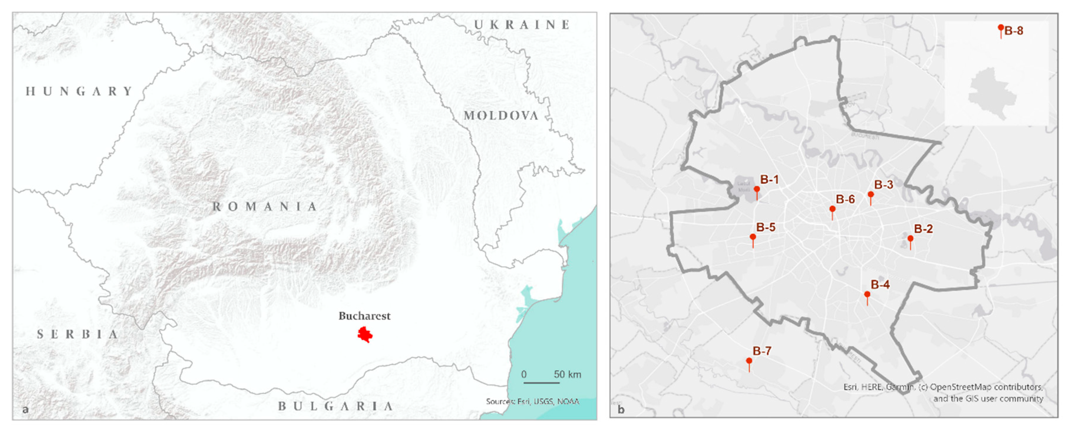
2.1. Study Area

Our analysis focuses on the European region, covering an area with a length of about 40 degrees latitude and 45 degrees longitude. According to Worldometer’s 2020 statistics [120], Europe ranks third among regions of the world, ordered by population, with 9.8% of the total world population [120]. Over 70% of the Europe population lives in urban areas [121], where the major exceedances of NO2 pollution occur.
Regarding the temporal dimension, the reference periods between 15 January and 30 April 2019 and 2020 were chosen according to the coronavirus pandemic evolution in Europe, in order to capture the transition from normal condition situation to the COVID-19 lockdown. The coronavirus pandemic in Europe started on 24 January, with the first declared case in France, but the lockdown was imposed first in the Lombardian region in Northern Italy on 8 March, followed by other regions in France, Spain, Germany, Romania, Poland, etc. On 13 March, the WHO declared Europe as an active center of COVID-19 pandemic, as the number of new cases became greater than in China.

2.2. Data Types and Sources

Sentinel-5P (S-5P) is a single satellite mission, as a part of the Global Monitoring for Environment and Security (GMES/Copernicus) program [122]. S-5P objective is to ensure the data continuity between previous SCIAMACHY, GOME-2, OMI, or Envisat missions and the upcoming Sentinel-5, providing information about atmospheric trace gases, aerosols, cloud distribution affecting air quality and climate, having a global daily coverage [72].
The TROPOsferic Monitoring Instrument, known as TROPOMI, is a passive sun backscatter imaging spectrometer that allows for the acquisitions of 8-band imagery, covering multiple spectral domains from UV and visible to near-infrared (NIR) and shortwave infrared (SWIR) [86]. Featuring a higher spatial resolution than its predecessors, of 7 × 3.5 km2 (along and across track), it offers a new potential for air quality research, making it suitable for polluting emission sources monitoring [87].
Collected on a large swath of 2600 km, the S-5P data are available to users at two different processing levels: L1B, as geolocated and radiometrically corrected TOA (top-of-atmosphere) radiances, and L2, in terms of multiple layers including radiance products, solar irradiance products and products for aerosols, clouds, and different pollutants (i.e., total columns of O3, SO2, NO2, CO, and CH4). Regarding the timeliness, the S-5P imagery is available on two services, as near-real time (NRT) in 3 h after sensing, and as nontime critical services with offline products (OFF) available with a delay of 12 h for L1B and 5 days for L2 products [123]. The S-5P L2-NO2 products are delivered in the netCDF format, allowing for the storage of multidimensional scientific information, including dimensions, variables/parameters, attributes, and coordinates.
In order to fulfil the aim of this paper, a total number of 492 offline L2-NO2 products were used (248 for 2019 and 244 for 2020), ensuring daily coverages for each temporal frame between 15 January to 30 Aprilin 2019 and 2020. These periods were selected in order to identify and compare the evolution of the NO2 concentrations during two different periods: under normal conditions and during the coronavirus pandemic outbreak. All the data were downloaded from the Copernicus Open Access Hub [124].
A second important dataset consists of NO2 ground-based measurements that were obtained from the international network of air quality monitoring stations. While the daily means concentrations in international units µg/m3 are available through the World Air Quality Index Project and the European Air Quality Index, hourly measurements were accessed from certain institutions that are responsible for data collection within an area or a country: UK-AIR, air quality information resource via Defra; Calidad del Air en Madrid, Servicio de Protección de la Atmósfera via EEA; Medi Ambient, Generalitat de Catalunya; Conselleria de Infraestructuras, Territorio y Medio Ambiente via EEA; Hessian State Office for Nature Conservation, Environment and Geology; Berlin Air Quality; AirParif (Association de surveillance de la qualité de l’air en Île-de-France); Agenzia Regionale per la Protezione dell’Ambiente della Lombardia; and Romanian National Environmental Protection Agency.
Economic and air traffic data from the European Commission (July 2020) were used in order to explain the effects of the COVID-19 lockdown measures on the European countries’ economy. Industrial Production Index (in %) indicates the changes in the production volume based on a reference year (2015).

2.3. Data Processing Methodology

The processing workflow of S-5P L2-NO2 data products was conducted through the free and open scalable platform of the Copernicus Research and User Support (RUS) Service [125,126], using Python languages together with HARP, VISAN, and QGIS software and following the methodology presented in the RUS Copernicus training on air quality monitoring [127].
The daily tropospheric NO2 column density was derived from the total columns of L2-NO2 products, converting the data from Level 2 processing to Level 3. This conversion is based on a series of parameters, referring at the same time to the dimensions (time, latitude, and longitude), variables (data names and data types), attributes, and coordinates. First, a spatial grid was established, covering the European region between 31 and 72 latitude degrees, with a spatial resolution of 0.05 × 0.05 degrees resulted from the resampling of the original product. Second, the data were filtered at a number density value quality over 75, in order to remove errors induced by clouds. Third, the daily tropospheric NO2 column number density was derived in international units of molecules/cm2, combining the products by time dimension, in order to obtain a single raster covering the entire study area. The 5-day and 10-day average tropospheric NO2 column density (molecules/cm2) mosaics were derived also using also the time dimension parameter, using an arithmetical mean of the cell values from stacked layers. Additionally, our analysis focuses on a case study from Bucharest, the capital of Romania, at the finer resolution of 0.01 × 0.01 degrees in order to illustrate the effects of the COVID-19 pandemic upon the NO2 pollution.
After the image processing steps and the derivation of the pollution parameter for the tropospheric NO2 column number density, a GIS (geographical information system) analysis was used in order to extract data from essential points such as the main industrial and urban centers most affected by the current outbreak.
The NO2 time-series values were extracted from both satellite-based and ground-based measurements on different locations for the January to April period. The statistical data were plotted in graphs, in order to analyze the correspondence of the NO2 trendline dynamics over time through visual comparison. The lines of best fit or trendlines were created as straight lines, in order to show the overall direction of the data. Statistics representing the variability of the daily tropospheric NO2 column values compared to the average value of the half-month, based on clear-sky days data collected by the TROPOMI sensor in 2019 and 2020, were plotted in order to show the seasonal characteristics, as well as the differences between the situation before and after the COVID-19 lockdown.
A cross-correlation analysis was used in order to validate the results and to statistically explain the correspondence between the TROPOMI spectrometric sensor NO2 calibrated measurement and the corresponding average from ground station measurements. Additionally, two statistical indicators were run in order to interpret the correlation results. First, p-value quantifies the idea of statistical significance of the evidence and is classified in percentage categories as follows: significant (<5%), marginally significant (<10%), and insignificant (>10%). Second, the Pearson correlation coefficient measures the linear correlation between both variables and is useful for identifying whether the correlations are linear positive (>0 … + 1), linear negative (−1 … <0), or if there is no linear correlation (0).

3. Results

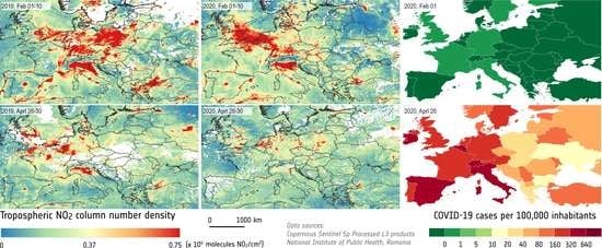
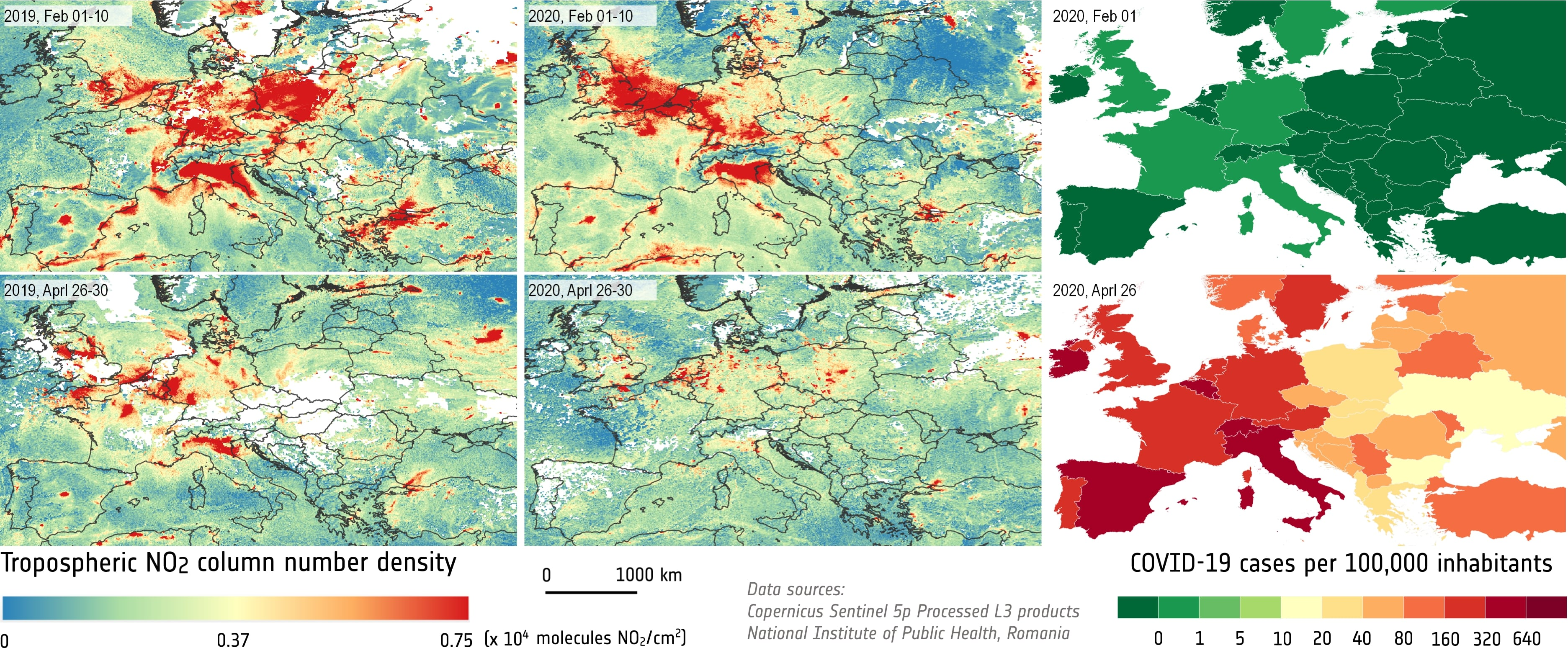
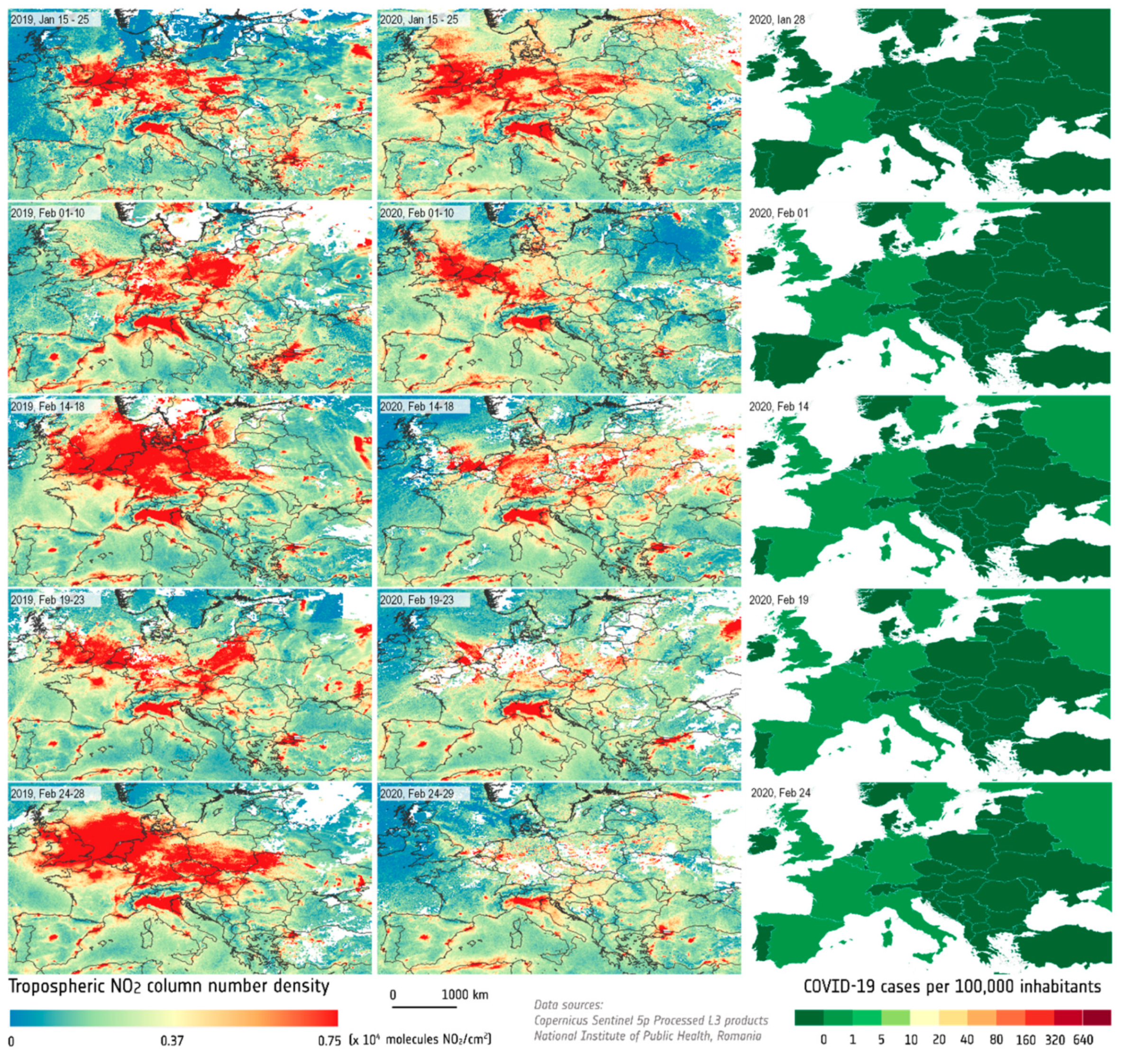
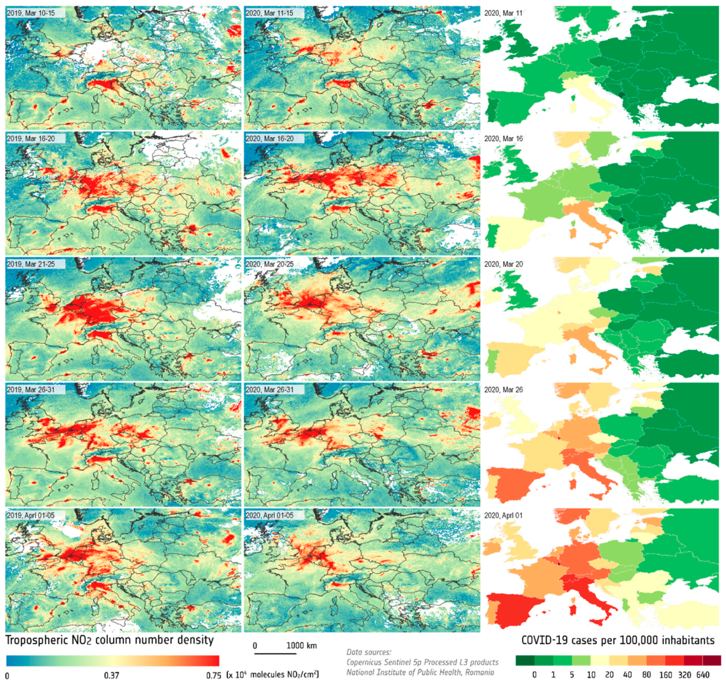
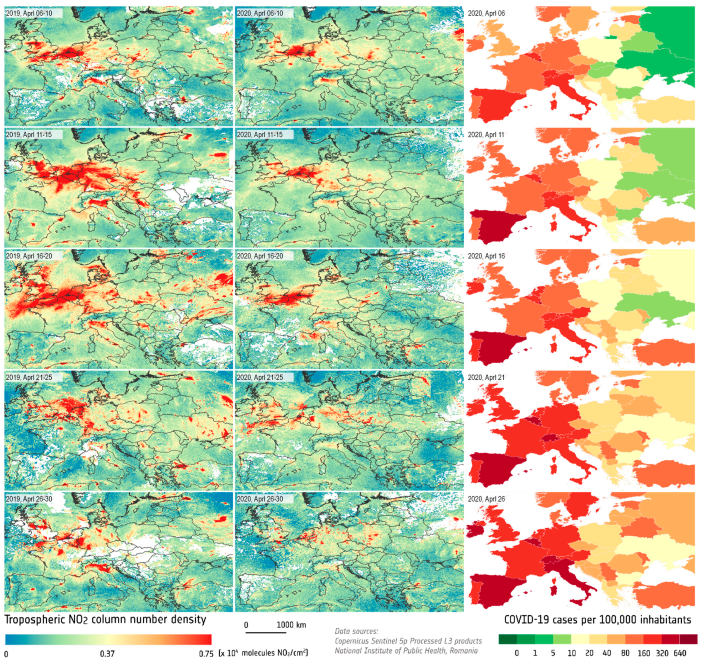
3.1. European Spatiotemporal Distribution of the NO2 Pollution

Our results on the NO2 gas monitoring over the European region highlight important changes between the temporal frames of the periods from 15 January to 30 April in 2019 and 2020. Comparative cartographic representations of the 5-, 6-, and 10-day average mosaics of the tropospheric NO2 column number density, extracted from Sentinel-5P imagery, were drawn for a better understanding of the spatial and temporal changes that occurred across Europe during the selected time spans.
The analyses of the maps and data from mid-January to the second 10-day period of February (Figure 1) reveal the fact that no considerable changes occurred between 2019 and 2020 with respect to the level of the NO2 pollution, as it maintains high values on large areas across Europe. This period corresponds to the normal condition of economic activities and the beginning of the COVID-19 epidemic in Europe, characterized by the occurrence of isolated cases in different countries. The differences can also be explained by the high dynamics of the NO2 gases in the atmosphere, as the wind can disperse the NO2 pollutants in less than 30 min [128].
The spatial repartition of the NO2 values clearly indicates two categories of NO2 pollution patterns over the Europe, with an intense contrast between them. The first pattern corresponds to large areas facing NO2 pollution issues, as it is the case of the remarkable Central and Northern European regions, including Germany, the Netherlands, Belgium, Northern France, the southern regions of Great Britain, Poland, and the northern part of the Czech Republic. This can be explained by the intensive industrial activities and vehicle traffic superposing on a dense transportation infrastructure network (mainly motorways and highways). Another large area facing NO2 pollution covers the Lombardian region territory in Northern Italy, where the tropospheric NO2 column number density maintains high values of about 0.75 × 10⁴ molecules/cm2 during the review periods.
The second category of NO2 distribution patterns is illustrated as strongly isolated hotspots of pollution covering big cities across Europe and their adjacent areas, following the same causes as mentioned previously. Cartographic results clearly indicate the large distribution of urban-polluted hotspots, not only in Western European cities such as Madrid, Barcelona, Valencia, Paris, Lyon, Marseille, and Rome, but also those in the Eastern Europe, including Istanbul, Bratislava, Budapest, Kiev, Moscow, Bucharest, and Belgrade.
The diachronic representations reveal the gradually remarkable decrease of NO2 pollution over Europe, starting from the end of February and at the beginning of March 2020, as it is shown by Figure 2, corresponding to the period when WHO declared the COVID-19 disease as a pandemic on 11 March, together with the coronavirus lockdown restrictions in multiple countries such as Italy, France, Spain, Romania, etc.
As an effect of the massive lockdown of industrial activity and vehicle traffic across Europe, NO2 pollution reduced considerably until the end of April as shown in Figure 3, being dominant overall, together with the improvement of air quality. By the end of April, multiple European cities that previously featured high levels of air pollution reported very good values of the air quality index, including NO2 parameters. Moreover, the NO2 polluted areas in Central and Northern Europe and the Lombardian region recorded considerable reductions of their spatial extent, and only some isolated hotspots corresponding to some active industries (e.g., power industry) still occur.
The regional analysis is also useful for understanding the spatial repartition of the NO2 pollution differences in Europe and the relationship between pollution sources and urban–industrial areas. From a geographical criteria point of view, the maps displayed above clearly highlight the direct relationship between urban and industrial areas and the NO2 pollution hotspots, confirming the hypotheses related to the main NO2 emission sources. Moreover, the cartographic representations illustrate the dominant role of the mountain ranges as well as the main air mass movements on pollutant distribution and dispersion. For instance, the Central and Northern European polluted areas follow the shape of the main air masses direction from the west to the east, and this can be observed too in other polluted areas in Poland or Ukraine. The Lombardian region is another example where geographically conditions put their imprints, as the mountain ranges and the main wind directions limit the spreading of NO2 gases and favor the increase of the pollution concentrations in the Po Plain.
Investigations conducted on NO2 pollution changes that occurred in Europe during the pandemic are more relevant for the identification of the effects of different pollution sources over the ambient air quality and finding practical solutions for environmental quality and population health status improvements, since air quality is one of the main priorities of the European Union.

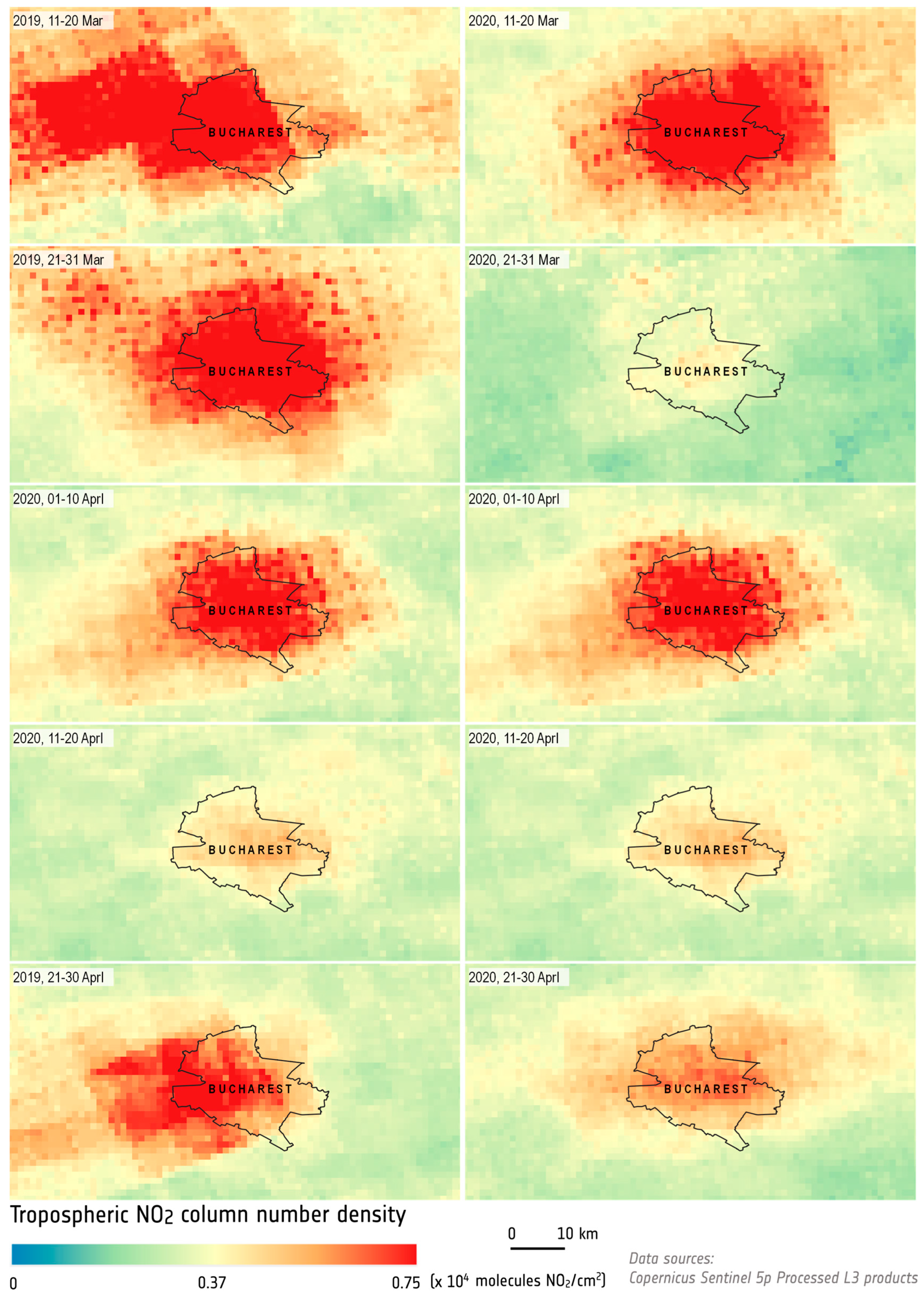
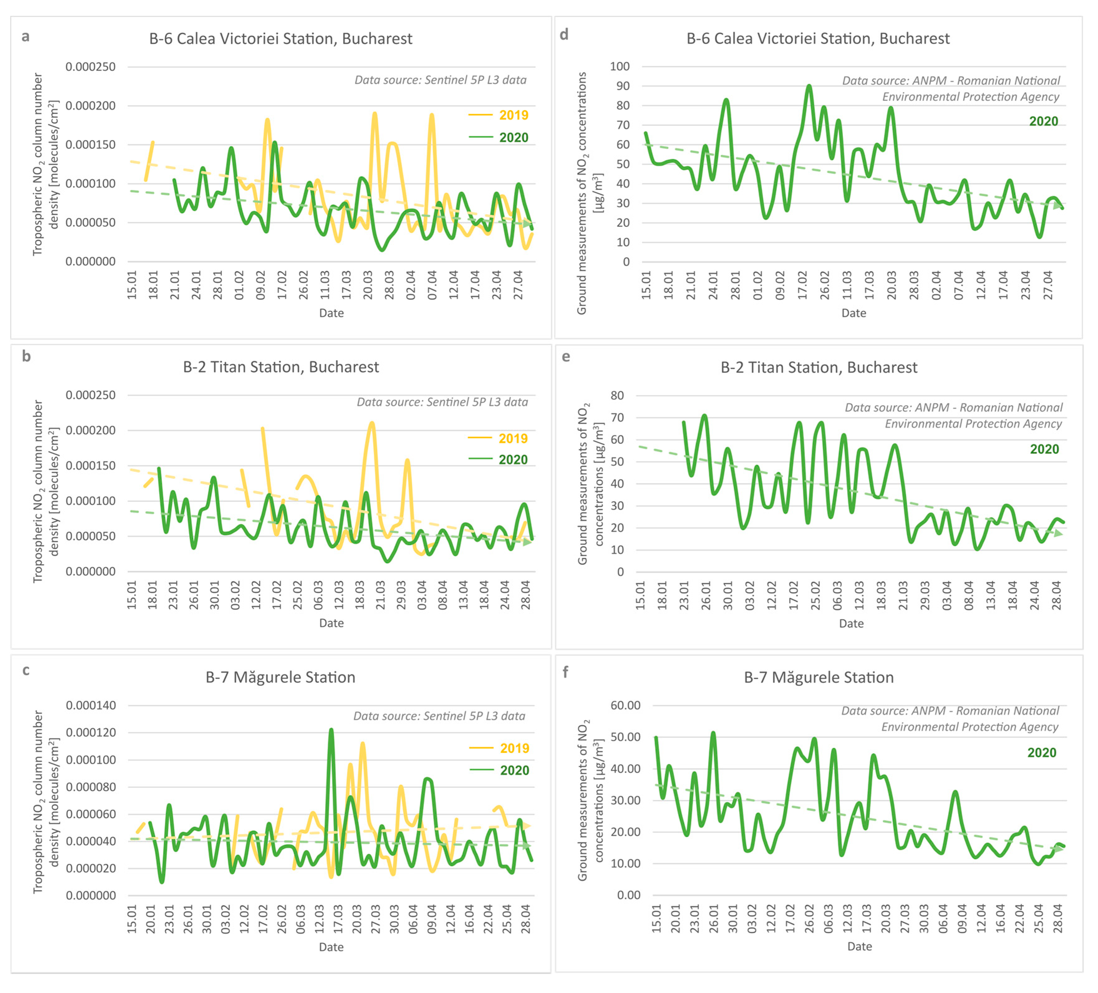
3.2. Local Scale NO2 Pollution Mapping and Assessment: A Case Study of Bucharest, Romania

A detailed assessment of NO2 pollution is also useful for local-scale analyses in order to better understand the role of pollution sources on air quality parameter definition. For this reason, we selected Bucharest, the capital city of Romania, as a case study (Figure 4), and at the same time it is one of the most polluted areas in Romania [129].
The tropospheric NO2 column number density generated from Sentinel-5P Level 3 imagery (Figure 5) illustrates overall the same trend of NO2 pollution during the 2020 coronavirus outbreak as with other cities from Europe, with several peculiarities. However, we can easily note the complexity of the NO2 pollution dynamics pattern, which features a temporal trend of a wave-like configuration. The 10-day average NO2 column number density highlights no substantial differences between 2019 and 2020, during the March–April period. For both temporal frames, there are 10-day periods of high level of the NO2 pollution alternating with 10-day periods with favorable values for NO2 pollutant parameters.
The 10-day periods between 11–20 March and 1–10 April are defined as anomalies, as there were generated accidental emissions that were caused by large waste dump sites fires on 10 March in the eastern part and on 8 April in the northwestern part of the capital city. These situations are reflected in the cartographic and statistical data as NO2 pollution peaks, as the road traffic and many economical activities were closed because of the COVID-19 outbreak. These anomalies raised the average values of the NO2 pollution for the several analyzed 10-day periods during the lockdown.

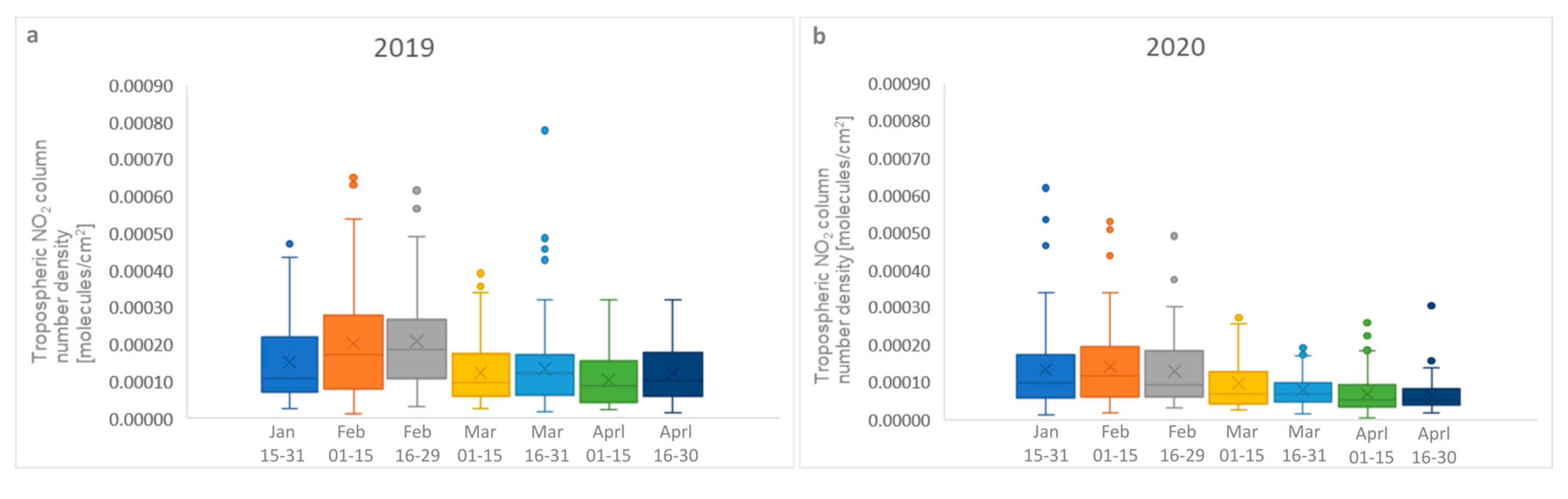
3.3. Quantitative Spatiotemporal Differences of NO2 Pollution Hotspots during the Pandemic Lockdown

The quantitative analyses of the NO2 pollution dynamics during the COVID-19 lockdown was based on geostatistical data processing of two datasets for a more concrete interpretation: S-5P satellite data tropospheric NO2 column number density (molecules/cm2) and the NO2 pollutants concentrations (µg/cm3) that resulted from ground station measurements. Observations on statistical data from selected cities across Europe confirmed the general trend of NO2 pollution reduction. The trendlines reveal decreases of the tropospheric NO2 column for 2020 compared to 2019, for all selected locations (Figure 6a–d or Figure 7a–d). This trend is confirmed by the ground measurements for 2020 (Figure 6e–h or Figure 7e–h). Regarding the Spanish cities (Figure 6), NO2 pollution decreased during the lockdown by 85% for Madrid, 78% for Valencia, and 75% for Barcelona, from the beginning of March to the end of April. In the northern regions of Italy, NO2 pollution decreased by 67% in Milano, while for other major European cities such as Paris, London, and Frankfurt, the decrease was between 36% and 40% (Figure 7).
The small differences on the graph dynamics between the satellite- and ground-based observations can be explained by the time shift between the sensing time of the S-5P sensor and the ground-based fixed hourly measurements. The distribution of the NO2 pollution can be influenced by the local climatic conditions [130]. The most important weather parameter is the wind regime, which can disperse pollutants in just a few minutes depending on wind speed and could transport them away from the emission sources [131]. Temperature is another climatic parameter to be considered, especially in situations of thermal inversions, when the warmer layer of air situated over the colder surface air works like a barrier, preventing the rise of the second one and favoring the increase of ambient air contamination [132]. This situation happens frequently over the cities located in mountain basins, as it is the case of Madrid and even Milano and Frankfurt. Moreover, high temperatures favor the photochemical reaction between NO2 and volatile organic compounds, leading to the formation of the ozone, as a secondary pollutant [133].
Temporal variations of the data can be observed in both observations datasets. For both periods, NO2 pollution records higher values in the winter season months (January–February) compared to the spring ones (March–April), as seen in Figure 8. This is a common situation as residential heating is an important source of NO2 emissions during the cold months. Moreover, a combination of high temperatures and solar radiation together with longer daylight time intervals favors the transformation of the NO2 gases to secondary pollutants (ozone) during the spring and summer seasons.
According to the Climate Copernicus Service [134], the 2019–2020 winter recorded higher surface temperatures compared to previous periods. In this regard, the surface temperature anomaly, with respect to the 1981–2010 average, was 3.24 °C in January 2020 and 3.85 °C in February 2020, while for the same months of the 2019 year, the anomalies were lower, namely 0.85 and 2.97 °C, respectively. For the March–April period, the surface temperature anomalies differences are lower, as follows: 2.52 and 1.50 °C for March and April 2020, respectively, compared to 2.34 and 1.56 °C for March and April 2019, respectively. However, the remarkable decrease of the NO2 pollution level in spring 2020, compared to the same period of the 2019 year, corresponds to the March–April COVID-19 outbreak. The outlier points on Figure 8 represents high values of the tropospheric NO2 column number density, which are very different from the standard deviation values of the time interval, corresponding to the most polluted days for the analyzed period.
For the Bucharest case study, we selected statistical data from three complementary ground stations (Figure 9), classified as urban traffic (B-6), urban background (B-2), and suburban (B-7), according to the international classification based on land use (L1) and type of transmitter source (L2). Bucharest registered a NO2 pollution reduction highlighted by the ground-based measurements of 76% at B-2 station, 64% at B-6 station, and 63% at B-7 station, during the review period from 15 January to 30 April 2020 (Figure 9e–g). The overall decrease trend is highlighted by the satellite-based measurements for the 2019 and 2020 January–April periods. The NO2 pollution differences between a normal reference situation (2019) and the COVID-19 lockdown (2020) are remarkable at the urban stations for the period between the start of March to mid-April. For the end of April 2019 and 2020, the NO2 values are quite similar, as the traffic activities returned to almost normal values (Figure 9a,b).

4. Discussion

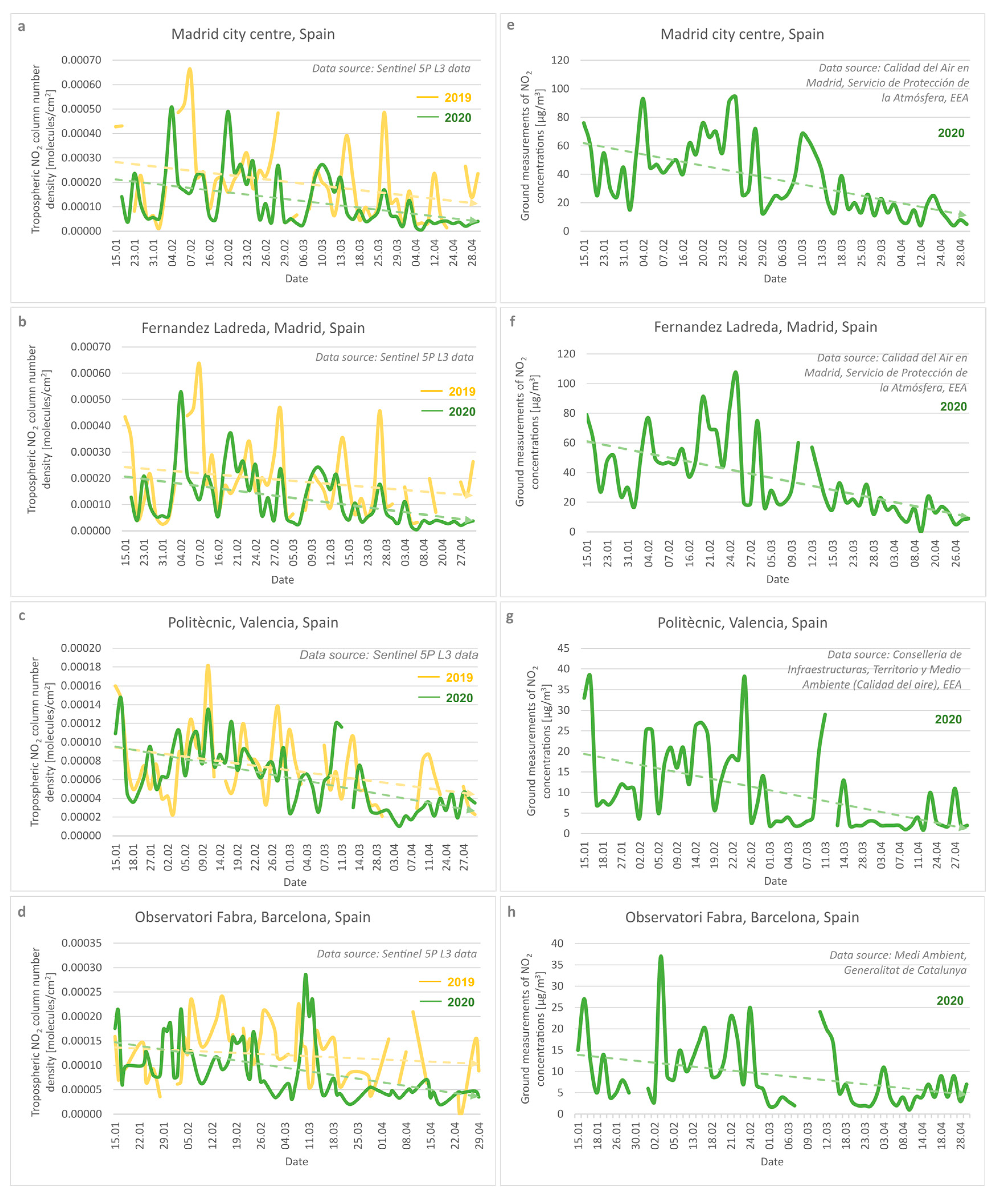
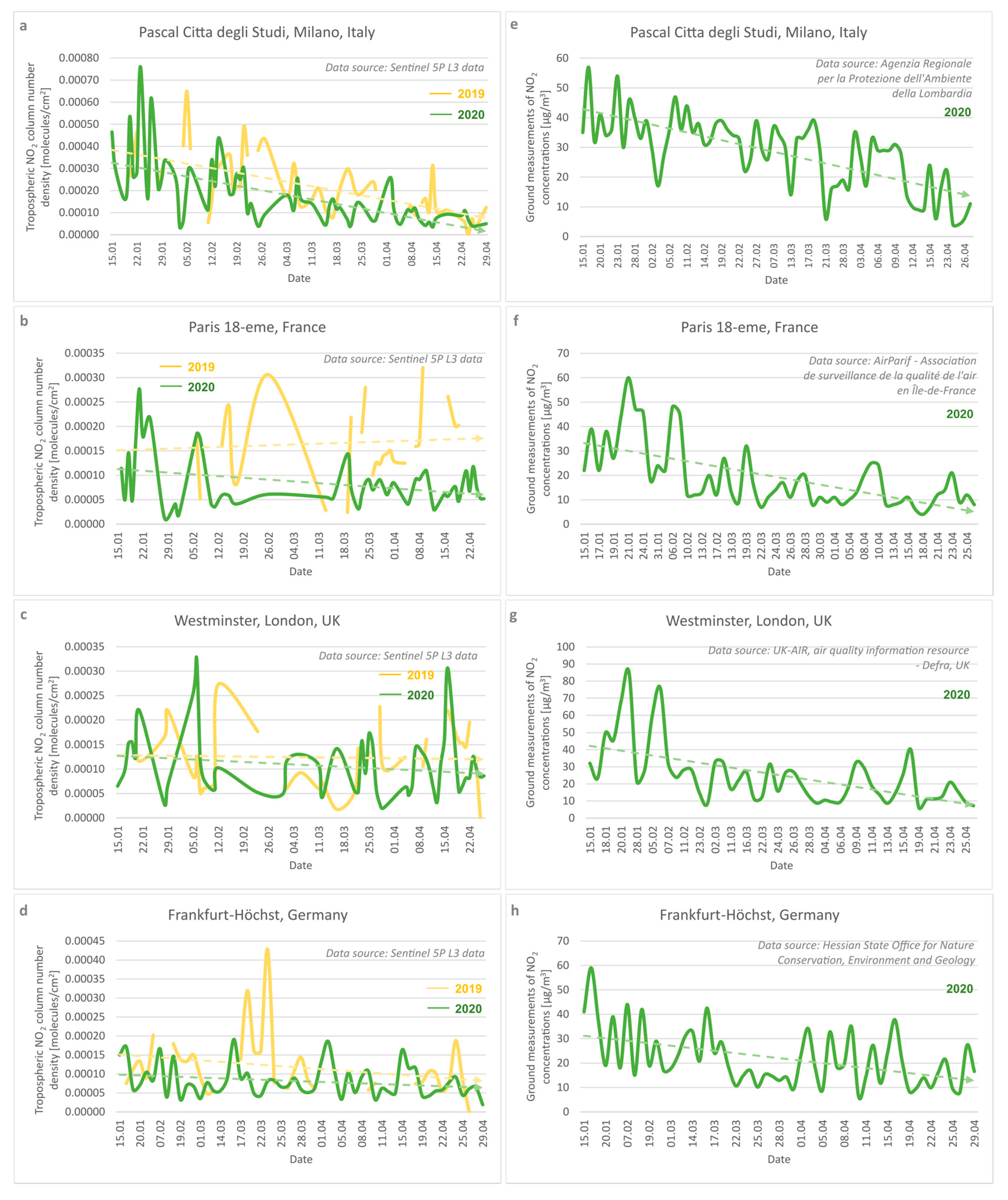
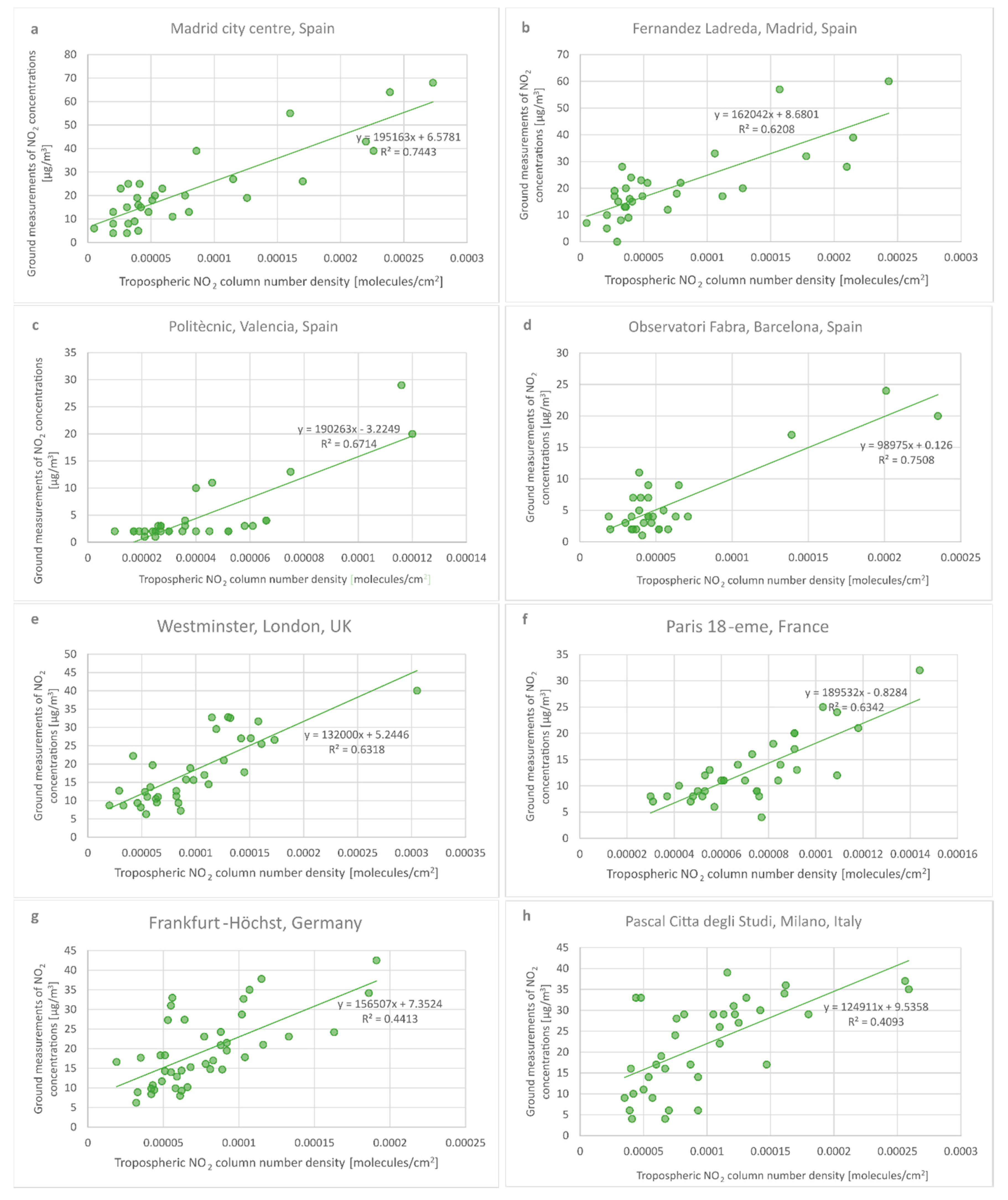
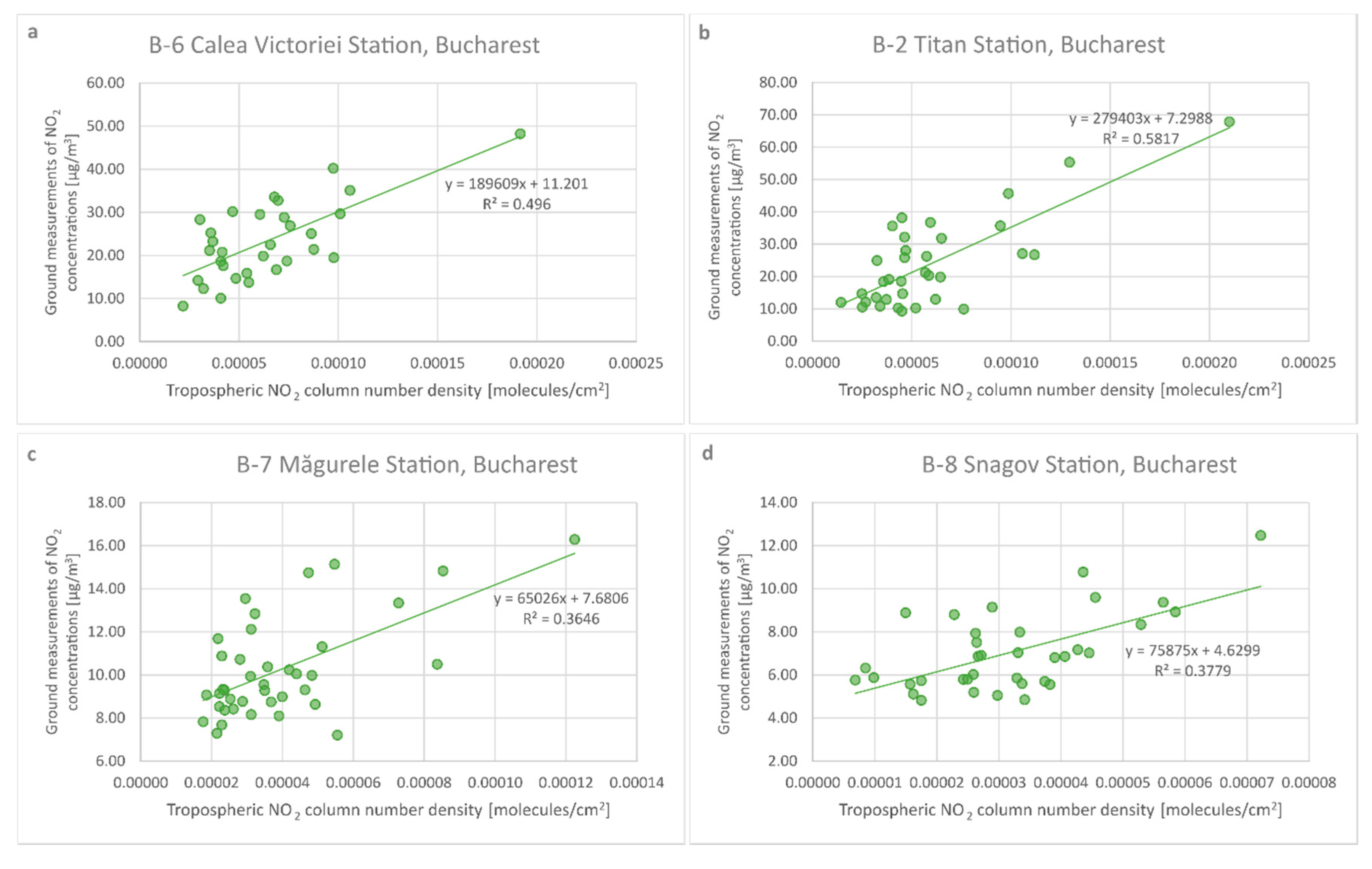
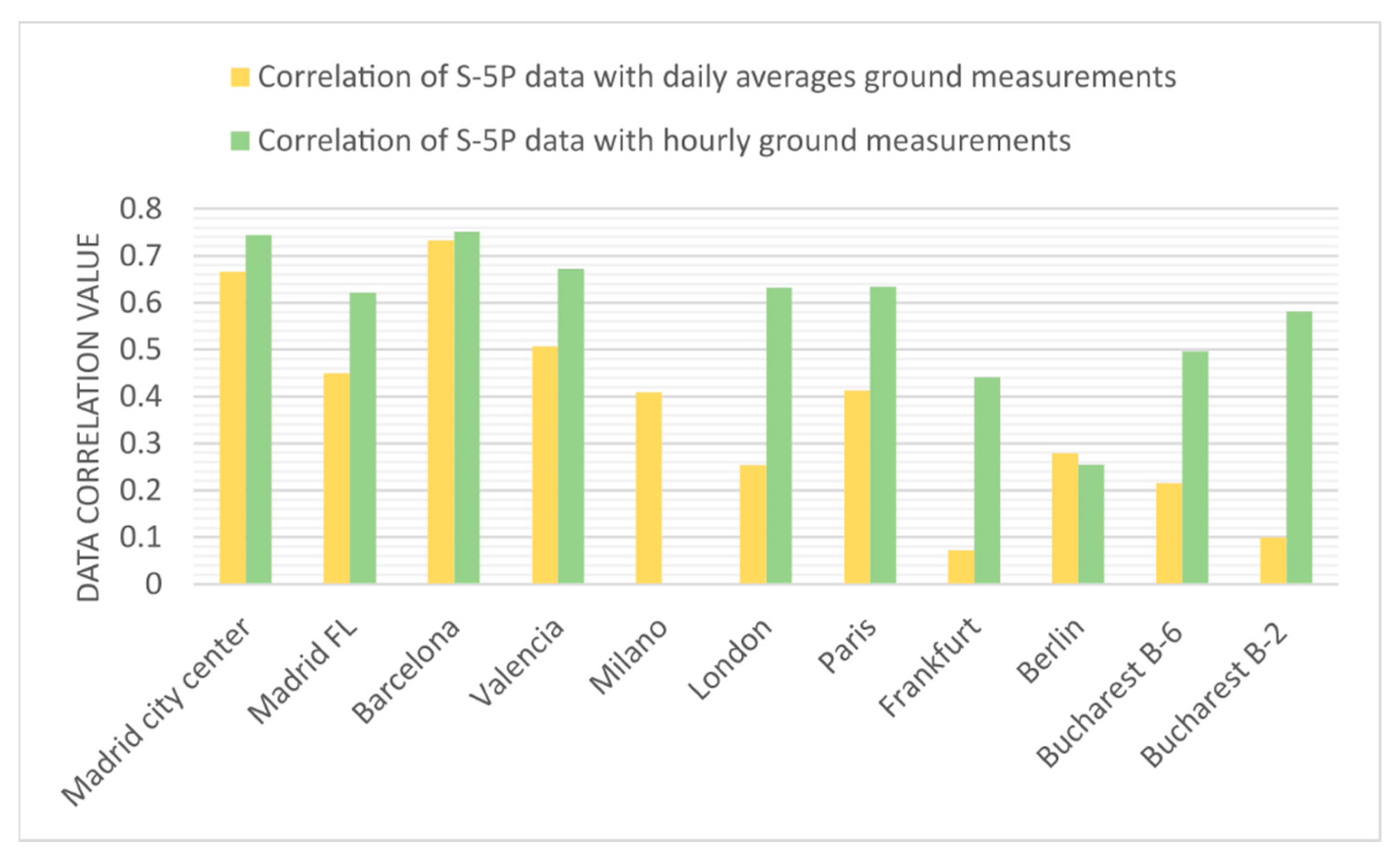
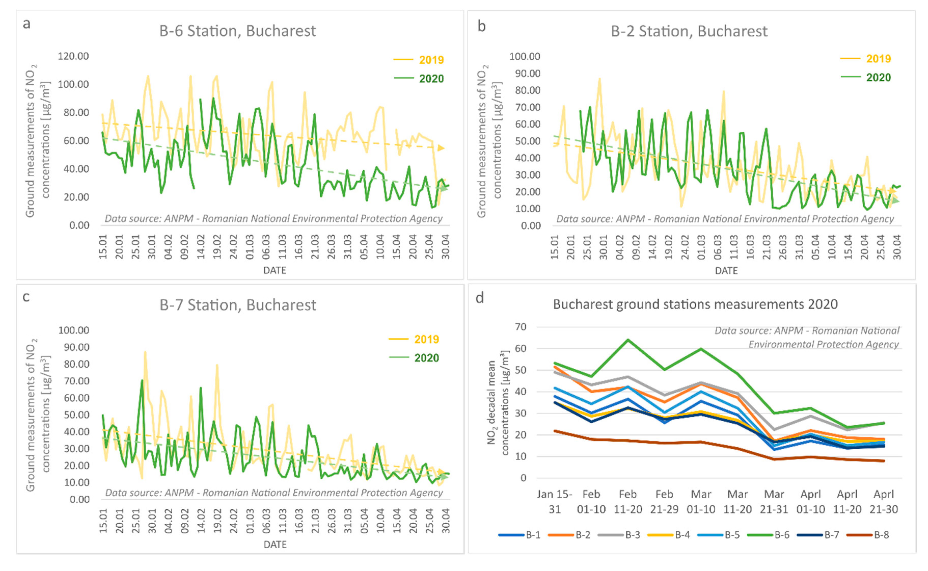
4.1. Cross-Correlation between Tropospheric NO2 TROPOMI-Based Data and Ground-Based Air Quality Station Measurements

Validation of the results confirms the reliability of the data and methodology employed on NO2 pollution monitoring. Therefore, the satellite-based TROPOMI products in terms of tropospheric NO2 column number density (molecules/cm2) were statistically correlated with independent datasets of ground-based NO2 concentrations measurements (µg/cm3), from selected hotspots across Europe on clear-sky days. The point locations correspond mainly to urban and suburban air quality monitoring stations.
The validation results illustrate medium to high correlation coefficients between both satellite- and ground-based data for many of the selected locations, with the R2 varying from 0.4413 (at Frankfurt-Höchst site) to 0.7518 (Observatori Fabra site in Barcelona), as seen in Figure 10. For the Milano station, the lower correlation of 0.4093 results from the use of NO2 daily averages ground data, as hourly measurements were not available.
For Bucharest, the correlation values are lower than those in other European cities, even when the data were extracted from enhanced resolution grids, up to 0.01 × 0.01 degrees. For instance, the higher correlation of 0.5817 was obtained for B-2 station (Figure 11b), which corresponds to a typical urban ground monitoring station, featured by a type of emergent source that is not specifically industrial or road traffic, followed by an urban-traffic station (B-6) that is situated in the Bucharest city center (Figure 11a). Lower correlation values correspond to suburban (B-7) and rural (B-8) stations (Figure 11c,d), which are situated outside of the city boundaries; the lower values may be because of possible discontinuities in data collection.
The resulted correlation values can be explained by the fact that the sensing time of Sentinel-5P data does not perfectly match the time when ground measurements were collected, as a time shift of up to 30 min, in some situations, is quite enough for the wind to disperse the NO2 pollutants [135]. As mentioned already, NO2 pollutants are easily dispersed under the influence of climatic conditions. We observed a direct relationship between the low correlation points and the wind speed values over 3 or 4 m/s. Because of NO2 gases’ potential conversion to secondary pollutants such as nitric acid and the ozone in the presence of humidity and sunlight, respectively, the correlation values increased when hourly ground measurements were used, closer to the S-5P sensing time instead of daily averages, as shown in Figure 12.
Another essential important argument for the data correlation values is concerned with the data gaps from the ground NO2 monitoring stations. This is a common situation when ground-based sensors did not record parameters for some temporal intervals, and the dataset is completed with averages values.
The quantitative analysis revealed the fact that low correlations are registered for stations from Central Europe, namely at Frankfurt, Berlin, Warsaw, and Prague. This happens because two offline L2 NO2 scene products were used in order to obtain complete coverages of Europe for each day. These scenes overlapping across Central Europe are stacked together in a single L3 NO2 dataset, storing the mean value between the two images, which were sensed at a time shift difference of about 2 h and 30 min. This situation can conduct to low correlation values compared to the ground measurements data.
The correlation results were statistically analyzed with the help of two indicators (Table 1). The correlation significance level was assessed by the p-value, which returned values under 5% for all of the encountered situations, indicating the fact that the correlations are significant. The Pearson correlation coefficient returned values between 0.597 and 0.865, highlighting that all correlations are positive linear.
In fact, according to some recent studies, the correlation values are quite similar with others obtained through different methods [136]. For instance, Ialongo, Virta, Eskes, Hovila, and Douros [87] obtained a correlation coefficient of 0.68 between satellite-based TROPOMI NO2 products derived data and ground-based observations in Helsinki (Finland). Moreover, they found out that the total columns underestimate ground-based observations, confirming our results. Lorente, Boersma, Eskes, Veefkind, van Geffen, de Zeeuw, Denier van der Gon, Beirle, and Krol [86] performed a complex investigation on TROPOMI NO2 validation over Paris, France, by integrating in situ measurements taken on the Eiffel Tower building in order to derive coincident NO2 columns based on the information on the atmospheric boundary layer height. The correlation coefficient of 0.88 reveals the fact that the validation results are better when using in situ measurements instead of ground-based data. Another complex investigation on TROPOMI NO2 data validation was carried out over the Greater Toronto area in Canada [89] through various approaches and different test sites, obtaining correlation coefficients between 0.65 to 0.89.

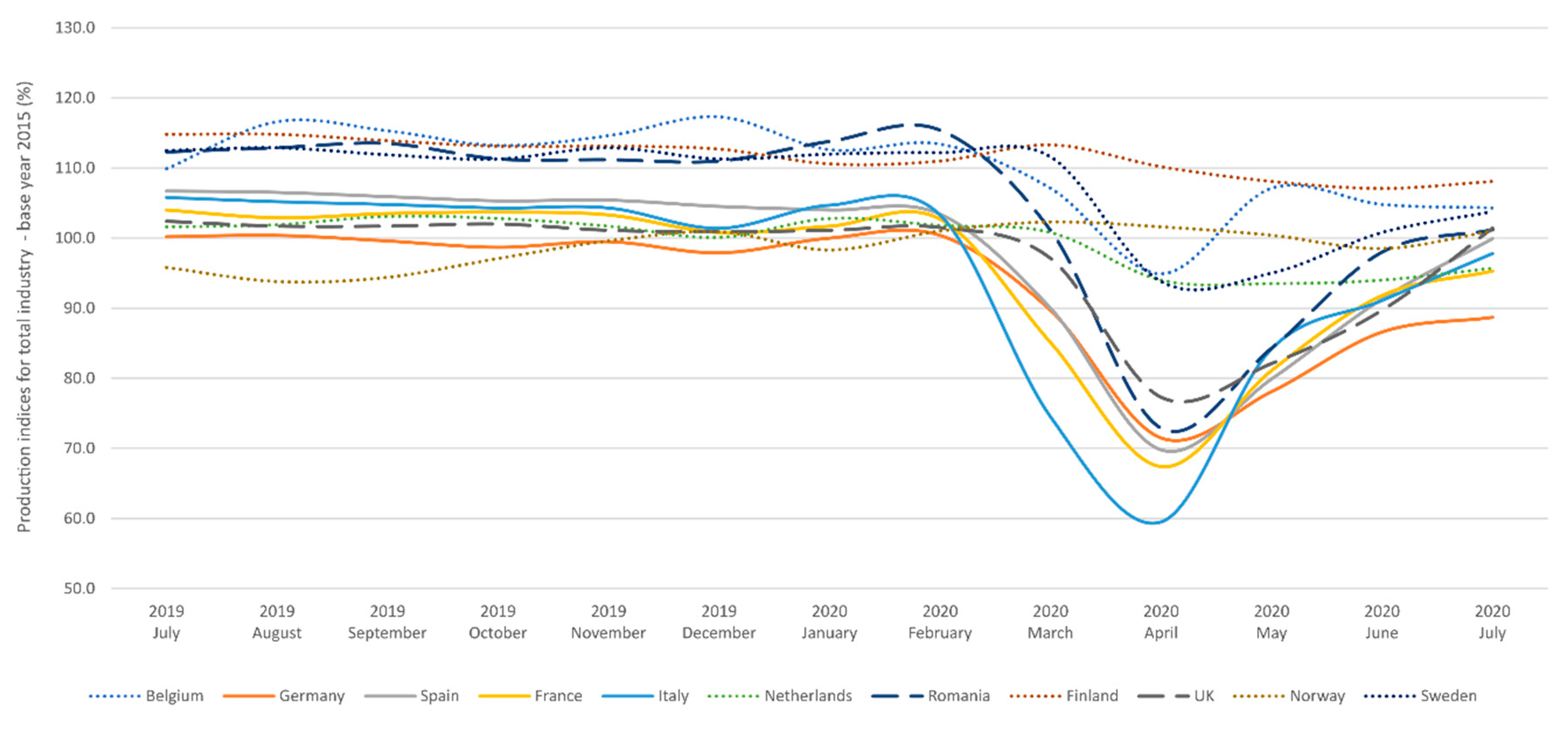
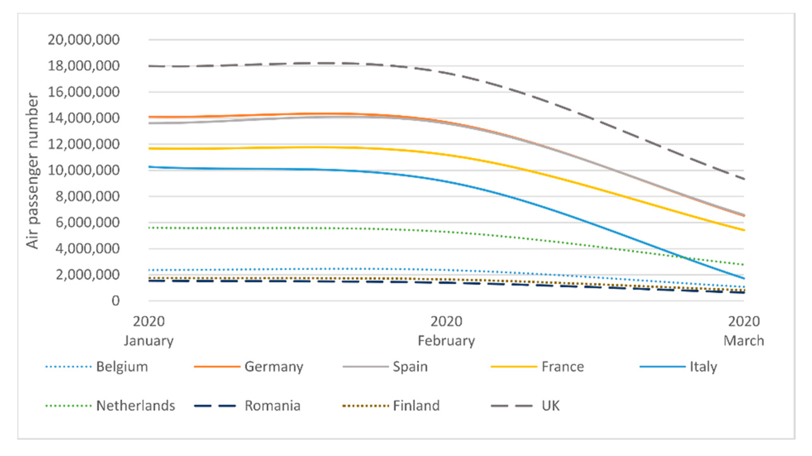
4.2. NO2 Pollution vs. COVID-19 Lockdown

At the European level, we observed a very high correspondence between NO2 emissions and COVID-19 confirmed cases (Figure 1, Figure 2 and Figure 3), with some regional variation. In this respect, three different situations were identified. First, the Southern European case, as the most affected region by the COVID-19 pandemic, is the area that registered a remarkable contrast of NO2 pollution values between 2019 and 2020. Countries like Spain and Italy reported between 320 and 640 cases per 100,000 inhabitants at the end of the April 2020 and, at the same time, they registered the highest number of deaths. Economic activities were drastically affected by the lockdown, as this situation was also being revealed by the substantial decrease of NO2 emissions. The former pollution hotspots corresponding to the biggest urban and industrial areas (Milan, Turin, Barcelona, Madrid, Bilbao, etc.) disappeared after the first 10-days (days 1 to 10) of March 2020. The Industrial Production Index (base year 2015) quantitatively highlights the reduction of economic activities, thus validating the results of our study (Figure 13). Comparing with the 2015 statistics, it can be observed that most of the European countries’ economies increased by 18% in the first two months of the year 2020. After the lockdown started, the industrial economies decreased by 40–45% in comparison with previous months. Moreover, the reduction of the pollution emissions caused by traffic activities corresponds with the air passenger number for the first three months of 2020 (Figure 14).
The second situation features countries such as France and the United Kingdom, where the socioeconomic activities continued until 23 March, when the statistics reveal a number of about 10,000 coronavirus confirmed cases. Figure 13 illustrates the temporal shift of the decline between European countries’ economies. The lockdown measure is reflected shortly after in the NO2 level of emissions. Starting from 1 April, the NO2 concentrations declined by zero in the United Kingdom, while in France the reduction was slight, with a small hotspot of NO2 emission maintained until mid-April.
The third situation corresponds to countries such as Belgium, the Netherlands, Luxembourg, Germany, Switzerland, and Austria, featured by a performant sanitary system. In these cases, the socioeconomic activities were not completely closed, but several prevention measures were adopted by limiting the nonessential activities. Therefore, the NO2 pollution decrease can be related to the vehicle traffic reduction and less to the economic activities. These countries were either indirectly affected by the economic decline of partner states in some cases (Norway, Finland, the Netherlands, Sweden), or they were less affected by the effect of closing some industrial domains or administrative units or districts, as was the case of Germany (Figure 13).
Romania suspended most of the socioeconomic activities starting on 11 March, when the statistics reported 29 confirmed cases and 0 deaths. This moment is reflected also by the Industrial Production Index, which illustrates an economic fall by about 40% between February 2020 and April 2020 (Figure 13). However, the ground-based air quality monitoring stations recorded declining values of NO2 pollutants, especially for the urban-traffic station in the city center of Bucharest (Figure 15a). The reduction impact was lower at the urban background (B-2 in Figure 15b), suburban (B-7 in Figure 15c), and rural (B-8 in Figure 15d) stations, where the traffic values were also lower under normal conditions. This situation reveals the fact that traffic-related activities remain the main emission source of NO2 pollution in Bucharest.
The overall decreasing trend of NO2 pollution, revealed by the ground-based observations between mid-January to the end of April in 2019 and 2020, highlights also the seasonality evolution of NO2 pollution, characterized by higher values in the cold months as an effect of the residential heating source.

5. Conclusions

In the latest years, the European Commission made remarkable efforts to reduce NO2 pollution and increase the population health state. In this respect, new policies together with new standard limit levels for different pollutants and plans were established for the mitigation of the effects of atmospheric pollution. Even if the level of NO2 pollution decreased constantly from 2003 to the present, there are still large areas where NO2 pollution level exceeds the standard limits imposed by the EU 2008 directive. Therefore, NO2 pollution monitoring is a crucial task in order to identify the emission sources and areas exposed, as well as to regulate air quality parameters.
The recently launched ESA Sentinel-5P satellite system produces free and open data products at high spatial resolution, available offline and near-real time in order to help air quality monitoring at different scales of analysis, from the big cities to national, continental, or global coverages. An even more important argument of the reliability of this data is the daily global coverage, which provides a continuous surface of data, showing the spatial distribution of different pollutants for a specific time. This offers a practical solution by gridding a large amount of spatial data since the ground-based air quality stations offer only punctual information. In addition, TROPOMI data can be successfully used for the accidental discharges of atmospheric pollutants modelling, as the case study on Bucharest reveals. However, there are some limitations in using Sentinel-5P data, such as the presence of clouds and the number of observations per day, which are not enough for a detailed monitoring as the pollutants can be easily dispersed into the atmosphere.
The Copernicus RUS Service provides free virtual machines and ready-to-use methodologies to help users get insights on data processing. The methodology proposed by the Copernicus RUS service and employed in this study is quite simple and easy to apply in order to derive geospatial data on different air pollutants.
Our study shows a general image of the NO2 pollution dynamics across the Europe, based on large volumes of Copernicus Sentinel-5P data processing. Moreover, this represents an example of a tool for various air pollutants monitoring and for decision making at the European, regional, national, and even local levels, according to the standards limits.
The COVID-19 lockdown is an example showing that the air pollutant level can be reduced and even controlled. The images collected after mid-March highlight a remarkable decrease of the NO2 pollution by 85% in some situations, as a result of the decrease of emissions from traffic or industrial activities, comparatively with the months before or with the same period from 2019.
The abrupt decrease of NO2 pollutant concentration over Europe from March to April 2020 was the direct effect of reactions by different official decision bodies at the state level against the COVID-19 pandemic. In this respect, three patterns can be identified: (1) countries severely affected by the pandemic, with a high level of infection rate in a short time and an important reduction of pollutant emissions; (2) countries with delayed restrictive measures; (3) countries where socioeconomic activities were partly restricted. Romania featured a significant reduction of current pollutants as a direct effect of road traffic limitation to essential needs. This is the reason the urban traffic monitoring stations in the Bucharest area recorded notable differences for NO2-related pollution.

Author Contributions

The authors M.V. and I.S. have equally contributed to the article. In more detail, the contributions for the different sections are as follows: Conceptualization, M.V. and C.N.; software, M.V.; validation, M.V., I.S. and R.D.; writing—original draft preparation, M.V., B.-A.M., I.S., C.N. and R.D.; writing—review and editing, M.V., I.S., B.-A.M., C.N. and R.D.; visualization, M.V. and I.S.; funding acquisition, M.V. All authors have read and agreed to the published version of the manuscript.

Funding

This research was partially funded by University of Bucharest.

Acknowledgments

This work was carried out using the resources made available by the Copernicus Research User Support (RUS) service (http://rus-copernicus.eu). RUS is a free service that aims at promoting the uptake of Copernicus data by providing cloud-based working environments customized to users’ needs, together with the support of technical and thematic experts as well as dedicated training resources. The service is funded by the European Commission, managed by the European Space Agency, and operated by CS Group and its partners.

Conflicts of Interest

The authors declare no conflict of interest. The funders had no role in the design of the study; in the collection, analyses, or interpretation of data; in the writing of the manuscript, or in the decision to publish the results.

References

  1. Meetham, A.R.; Bottom, D.; Cayton, S. Atmospheric Pollution: Its History, Origins and Prevention; Elsevier: Amsterdam, The Netherlands, 2016. [Google Scholar]
  2. Olmo, N.R.S.; Saldiva, P.; Braga, A.L.F.; Lin, C.A.; Santos, U.D.P.; Pereira, L.A. A review of low-level air pollution and adverse effects on human health: Implications for epidemiological studies and public policy. Clinics 2011, 66, 681–690. [Google Scholar] [CrossRef] [PubMed] [Green Version]
  3. Sokhi, R.; Kitwiroon, N. Air pollution in urban areas. In World Atlas of Atmospheric Pollution; Anthem Press: London, UK, 2011; pp. 19–34. [Google Scholar]
  4. Lavaine, E. An Econometric Analysis of Atmospheric Pollution, Environmental Disparities and Mortality Rates. Environ. Resour. Econ. 2014, 60, 215–242. [Google Scholar] [CrossRef]
  5. World Health Organization. Air Pollution. Available online: https://www.who.int/health-topics/air-pollution#tab=tab_1 (accessed on 14 August 2020).
  6. Raaschou-Nielsen, O.; Andersen, Z.J.; Beelen, R.; Samoli, E.; Stafoggia, M.; Weinmayr, G.; Hoffmann, B.; Fischer, P.; Nieuwenhuijsen, M.J.; Brunekreef, B.; et al. Air pollution and lung cancer incidence in 17 European cohorts: Prospective analyses from the European Study of Cohorts for Air Pollution Effects (ESCAPE). Lancet Oncol. 2013, 14, 813–822. [Google Scholar] [CrossRef]
  7. Perez, L.; Declercq, C.; Iñiguez, C.; Aguilera, I.; Badaloni, C.; Ballester, F.; Bouland, C.; Chanel, O.; Cirarda, F.B.; Forastiere, F.; et al. Chronic burden of near-roadway traffic pollution in 10 European cities (APHEKOM network). Eur. Respir. J. 2013, 42, 594–605. [Google Scholar] [CrossRef] [Green Version]
  8. Cesaroni, G.; Forastiere, F.; Stafoggia, M.; Andersen, Z.J.; Badaloni, C.; Beelen, R.; Caracciolo, B.; De Faire, U.; Erbel, R.; Eriksen, K.T.; et al. Long term exposure to ambient air pollution and incidence of acute coronary events: Prospective cohort study and meta-analysis in 11 European cohorts from the ESCAPE Project. BMJ 2014, 348, f7412. [Google Scholar] [CrossRef] [Green Version]
  9. Slama, R.; Bottagisi, S.; Solansky, I.; Lepeule, J.; Giorgis-Allemand, L.; Sram, R. Short-Term Impact of Atmospheric Pollution on Fecundability. Epidemiology 2013, 24, 871–879. [Google Scholar] [CrossRef]
  10. Vidotto, J.P.; Pereira, L.A.A.; Braga, A.L.F.; Silva, C.A.; Sallum, A.M.; Campos, L.M.; Martins, L.C.; Farhat, S.C.L. Atmospheric pollution: Influence on hospital admissions in paediatric rheumatic diseases. Lupus 2012, 21, 526–533. [Google Scholar] [CrossRef]
  11. Baldasano, J.M. COVID-19 lockdown effects on air quality by NO2 in the cities of Barcelona and Madrid (Spain). Sci. Total Environ. 2020, 741, 140353. [Google Scholar] [CrossRef]
  12. World Health Organization. Health Aspects of Air Pollution with Particulate Matter, Ozone and Nitrogen Dioxide; WHO: Bonn, Germany, 2003; p. 98. [Google Scholar]
  13. Li, Y.; Wang, Y.; Rui, X.; Li, Y.; Li, Y.; Wang, H.; Zuo, J.; Tong, Y. Sources of atmospheric pollution: A bibliometric analysis. Scientometrics 2017, 112, 1025–1045. [Google Scholar] [CrossRef]
  14. WAKI. Available online: https://waqi.info/ (accessed on 29 July 2020).
  15. AIRINDEX. Available online: https://airindex.eea.europa.eu/Map/AQI/Viewer/ (accessed on 5 June 2020).
  16. EC. Available online: https://ec.europa.eu/environment/air/quality/standards.htm (accessed on 18 May 2020).
  17. EEA. Air Quality in Europe; European Environment Agency, Publications Office of the European Union: Luxembourg, 2019; p. 99. [Google Scholar]
  18. Gentner, D.R.; Jathar, S.H.; Gordon, T.D.; Bahreini, R.; Day, D.A.; El Haddad, I.; Hayes, P.L.; Pieber, S.M.; Platt, S.M.; De Gouw, J.; et al. Review of Urban Secondary Organic Aerosol Formation from Gasoline and Diesel Motor Vehicle Emissions. Environ. Sci. Technol. 2017, 51, 1074–1093. [Google Scholar] [CrossRef]
  19. Salvador, P.; Artiñano, B.; Viana, M.; Querol, X.; Alastuey, A.; Gonzalez–Fernandez, I.; Alonso, R. Spatial and temporal variations in PM10 and PM2.5 across Madrid metropolitan area in 1999–2008. Procedia Environ. Sci. 2011, 4, 198–208. [Google Scholar] [CrossRef] [Green Version]
  20. Nagpure, A.S.; Gurjar, B.R.; Martel, J. Human health risks in national capital territory of Delhi due to air pollution. Atmos. Pollut. Res. 2014, 5, 371–380. [Google Scholar] [CrossRef] [Green Version]
  21. Sindhwani, R.; Goyal, P. Assessment of traffic-generated gaseous and particulate matter emissions and trends over Delhi (2000–2010). Atmos. Pollut. Res. 2014, 5, 438–446. [Google Scholar] [CrossRef] [Green Version]
  22. European Environment Agency. Available online: http://www.eea.europa.eu/ (accessed on 16 December 2011).
  23. Amann, M.; Bertok, I.; Borken-Kleefeld, J.; Cofala, J.; Heyes, C.; Höglund-Isaksson, L.; Klimont, Z.; Nguyen, B.; Posch, M.; Rafaj, P.; et al. Cost-effective control of air quality and greenhouse gases in Europe: Modeling and policy applications. Environ. Model. Softw. 2011, 26, 1489–1501. [Google Scholar] [CrossRef]
  24. Sicard, P.; Lesne, O.; Alexandre, N.; Mangin, A.; Collomp, R. Air quality trends and potential health effects—Development of an aggregate risk index. Atmos. Environ. 2011, 45, 1145–1153. [Google Scholar] [CrossRef]
  25. Sicard, P.; Talbot, C.; Lesne, O.; Mangin, A.; Alexandre, N.; Collomp, R. The Aggregate Risk Index: An intuitive tool providing the health risks of air pollution to health care community and public. Atmos. Environ. 2012, 46, 11–16. [Google Scholar] [CrossRef]
  26. Escudero, M.; Lozano, A.; Hierro, J.; Tapia, O.; Del Valle, J.; Alastuey, A.; Moreno, T.; Anzano, J.; Querol, X. Assessment of the variability of atmospheric pollution in National Parks of mainland Spain. Atmos. Environ. 2016, 132, 332–344. [Google Scholar] [CrossRef] [Green Version]
  27. Fotourehchi, Z. Health effects of air pollution: An empirical analysis for developing countries. Atmos. Pollut. Res. 2016, 7, 201–206. [Google Scholar] [CrossRef]
  28. Bougoudis, I.; Demertzis, K.; Iliadis, L.; Anezakis, V.-D.; Papaleonidas, A. Semi-supervised Hybrid Modeling of Atmospheric Pollution in Urban Centers. In International Conference on Engineering Applications of Neural Networks; Springer: Cham, Switherlands, 2016; pp. 51–63. [Google Scholar]
  29. Bougoudis, I.; Demertzis, K.; Iliadis, L. HISYCOL a hybrid computational intelligence system for combined machine learning: The case of air pollution modeling in Athens. Neural Comput. Appl. 2015, 27, 1191–1206. [Google Scholar] [CrossRef]
  30. Gulia, S.; Nagendra, S.S.; Khare, M.; Khanna, I. Urban air quality management-A review. Atmos. Pollut. Res. 2015, 6, 286–304. [Google Scholar] [CrossRef] [Green Version]
  31. Xing, J.; Mathur, R.; Pleim, J.; Hogrefe, C.; Gan, C.-M.; Wong, D.C.; Wei, C.; Gilliam, R.; Pouliot, G. Observations and modeling of air quality trends over 1990–2010 across the Northern Hemisphere: China, the United States and Europe. Atmos. Chem. Phys. Discuss. 2015, 15, 2723–2747. [Google Scholar] [CrossRef] [Green Version]
  32. Vardoulakis, S.; Solazzo, E.; Lumbreras, J. Intra-urban and street scale variability of BTEX, NO2 and O3 in Birmingham, UK: Implications for exposure assessment. Atmos. Environ. 2011, 45, 5069–5078. [Google Scholar] [CrossRef]
  33. Robinson, D.; Lloyd, C.; McKinley, J. Increasing the accuracy of nitrogen dioxide (NO2) pollution mapping using geographically weighted regression (GWR) and geostatistics. Int. J. Appl. Earth Obs. Geoinf. 2013, 21, 374–383. [Google Scholar] [CrossRef]
  34. Menut, L.; Bessagnet, B.; Khvorostyanov, D.; Beekmann, M.; Blond, N.; Colette, A.; Coll, I.; Curci, G.; Foret, G.; Hodzic, A.; et al. CHIMERE 2013: A model for regional atmospheric composition modelling. Geosci. Model Dev. 2013, 6, 981–1028. [Google Scholar] [CrossRef] [Green Version]
  35. Janssens-Maenhout, G.; Crippa, M.; Guizzardi, D.; Dentener, F.; Muntean, M.; Pouliot, G.; Keating, T.; Zhang, Q.; Kurokawa, J.; Wankmüller, R.; et al. HTAP_v2.2: A mosaic of regional and global emission grid maps for 2008 and 2010 to study hemispheric transport of air pollution. Atmos. Chem. Phys. Discuss. 2015, 15, 11411–11432. [Google Scholar] [CrossRef] [Green Version]
  36. Beelen, R.; Hoek, G.; Vienneau, D.; Eeftens, M.; Dimakopoulou, K.; Pedeli, X.; Tsai, M.-Y.; Künzli, N.; Schikowski, T.; Marcon, A.; et al. Development of NO2 and NOx land use regression models for estimating air pollution exposure in 36 study areas in Europe—The ESCAPE project. Atmos. Environ. 2013, 72, 10–23. [Google Scholar] [CrossRef]
  37. Beckerman, B.; Jerrett, M.; Martin, R.V.; Van Donkelaar, A.; Ross, Z.; Burnett, R.T. Application of the deletion/substitution/addition algorithm to selecting land use regression models for interpolating air pollution measurements in California. Atmos. Environ. 2013, 77, 172–177. [Google Scholar] [CrossRef]
  38. Ma, J.; Beirle, S.; Jin, J.; Shaiganfar, R.; Yan, P.; Wagner, T. Tropospheric NO2 vertical column densities over Beijing: Results of the first three years of ground-based MAX-DOAS measurements (2008–2011) and satellite validation. Atmos. Chem. Phys. 2013, 13, 1547–1567. [Google Scholar] [CrossRef] [Green Version]
  39. Morgan, W.T.; Allan, J.D.; Bower, K.; Highwood, E.J.; Liu, D.; Mcmeeking, G.R.; Northway, M.J.; Williams, P.I.; Krejci, R.; Coe, H. Airborne measurements of the spatial distribution of aerosol chemical composition across Europe and evolution of the organic fraction. Atmos. Chem. Phys. Discuss. 2010, 10, 4065–4083. [Google Scholar] [CrossRef] [Green Version]
  40. Novotny, E.V.; Bechle, M.J.; Millet, D.B.; Marshall, J.D. National satellite-based land-use regression: NO2 in the United States. Environ. Sci. Technol. 2011, 45, 4407–4414. [Google Scholar] [CrossRef]
  41. Colette, A.; Granier, C.; Hodnebrog, Ø.; Jakobs, H.; Maurizi, A.; Nyiri, A.; Bessagnet, B.; d’Angiola, A.; d’Isidoro, M.; Gauss, M. Air quality trends in Europe over the past decade: A first multi-model assessment. Atmos. Chem. Phys. 2011, 11, 11657–11678. [Google Scholar] [CrossRef] [Green Version]
  42. Pouliot, G.; Pierce, T.; Van Der Gon, H.D.; Schaap, M.; Moran, M.; Nopmongcol, U. Comparing emission inventories and model-ready emission datasets between Europe and North America for the AQMEII project. Atmos. Environ. 2012, 53, 4–14. [Google Scholar] [CrossRef]
  43. de Hoogh, K.; Gulliver, J.; van Donkelaar, A.; Martin, R.V.; Marshall, J.D.; Bechle, M.J.; Cesaroni, G.; Pradas, M.C.; Dedele, A.; Eeftens, M. Development of West-European PM2.5 and NO2 land use regression models incorporating satellite-derived and chemical transport modelling data. Environ. Res. 2016, 151, 1–10. [Google Scholar] [CrossRef] [Green Version]
  44. Liu, W.; Li, X.; Chen, Z.; Zeng, G.; León, T.; Liang, J.; Huang, G.; Gao, Z.; Jiao, S.; He, X.; et al. Land use regression models coupled with meteorology to model spatial and temporal variability of NO2 and PM10 in Changsha, China. Atmos. Environ. 2015, 116, 272–280. [Google Scholar] [CrossRef]
  45. Brandt, J.; Silver, J.; Frohn, L.; Geels, C.; Gross, A.; Hansen, A.; Hansen, K.M.; Hedegaard, G.; Skjoth, C.A.; Villadsen, H.; et al. An integrated model study for Europe and North America using the Danish Eulerian Hemispheric Model with focus on intercontinental transport of air pollution. Atmos. Environ. 2012, 53, 156–176. [Google Scholar] [CrossRef]
  46. Carvalho, A.; Monteiro, A.; Solman, S.; Miranda, A.I.; Borrego, C. Climate-driven changes in air quality over Europe by the end of the 21st century, with special reference to Portugal. Environ. Sci. Policy 2010, 13, 445–458. [Google Scholar] [CrossRef] [Green Version]
  47. Kumar, U.; Jain, V.K. ARIMA forecasting of ambient air pollutants (O3, NO, NO2 and CO). Stoch. Environ. Res. Risk Assess. 2009, 24, 751–760. [Google Scholar] [CrossRef]
  48. Shu, Y.; Lam, N.S. Spatial disaggregation of carbon dioxide emissions from road traffic based on multiple linear regression model. Atmos. Environ. 2011, 45, 634–640. [Google Scholar] [CrossRef]
  49. Viana, M.; Hammingh, P.; Colette, A.; Querol, X.; Degraeuwe, B.; De Vlieger, I.; Van Aardenne, J. Impact of maritime transport emissions on coastal air quality in Europe. Atmos. Environ. 2014, 90, 96–105. [Google Scholar] [CrossRef]
  50. Ji, M.; Jiang, Y.; Han, X.; Liu, L.; Xu, X.; Qiao, Z.; Sun, W. Spatiotemporal Relationships between Air Quality and Multiple Meteorological Parameters in 221 Chinese Cities. Complexity 2020, 2020, 1–25. [Google Scholar] [CrossRef]
  51. Allen, R.W.; Amram, O.; Wheeler, A.J.; Brauer, M. The transferability of NO and NO2 land use regression models between cities and pollutants. Atmos. Environ. 2011, 45, 369–378. [Google Scholar] [CrossRef]
  52. Duncan, B.N.; Prados, A.I.; Lamsal, L.N.; Liu, Y.; Streets, D.G.; Gupta, P.; Hilsenrath, E.; Kahn, R.A.; Nielsen, J.E.; Beyersdorf, A.J.; et al. Satellite data of atmospheric pollution for U.S. air quality applications: Examples of applications, summary of data end-user resources, answers to FAQs, and common mistakes to avoid. Atmos. Environ. 2014, 94, 647–662. [Google Scholar] [CrossRef] [Green Version]
  53. Li, J. Pollution Trends in China from 2000 to 2017: A Multi-Sensor View from Space. Remote Sens. 2020, 12, 208. [Google Scholar] [CrossRef] [Green Version]
  54. Popp, T.; Hegglin, M.I.; Hollmann, R.; Ardhuin, F.; Bartsch, A.; Bastos, A.; Bennett, V.; Boutin, J.; Brockmann, C.; Buchwitz, M.; et al. Consistency of satellite climate data records for Earth system monitoring. Bull. Am. Meteorol. Soc. 2020, 1–68. [Google Scholar] [CrossRef]
  55. Streets, D.G.; Canty, T.; Carmichael, G.R.; De Foy, B.; Dickerson, R.R.; Duncan, B.N.; Edwards, D.P.; Haynes, J.A.; Henze, D.K.; Houyoux, M.R.; et al. Emissions estimation from satellite retrievals: A review of current capability. Atmos. Environ. 2013, 77, 1011–1042. [Google Scholar] [CrossRef] [Green Version]
  56. Van Donkelaar, A.; Martin, R.V.; Brauer, M.; Kahn, R.; Levy, R.; Verduzco, C.; Villeneuve, P.J. Global Estimates of Ambient Fine Particulate Matter Concentrations from Satellite-Based Aerosol Optical Depth: Development and Application. Environ. Health Perspect. 2010, 118, 847–855. [Google Scholar] [CrossRef] [Green Version]
  57. Chudnovsky, A.A.; Kostinski, A.; Lyapustin, A.; Koutrakis, P. Spatial scales of pollution from variable resolution satellite imaging. Environ. Pollut. 2013, 172, 131–138. [Google Scholar] [CrossRef] [PubMed]
  58. Zheng, Y.; Zhang, Q.; Liu, Y.; Geng, G.; He, K. Estimating ground-level PM2.5 concentrations over three megalopolises in China using satellite-derived aerosol optical depth measurements. Atmos. Environ. 2016, 124, 232–242. [Google Scholar] [CrossRef]
  59. Li, Y.; Lin, C.; Lau, A.K.H.; Liao, C.; Zhang, Y.; Zeng, W.; Li, C.; Fung, J.C.; Tse, T.K.T. Assessing Long-Term Trend of Particulate Matter Pollution in the Pearl River Delta Region Using Satellite Remote Sensing. Environ. Sci. Technol. 2015, 49, 11670–11678. [Google Scholar] [CrossRef]
  60. Bai, K.; Ma, M.; Chang, N.-B.; Gao, W. Spatiotemporal trend analysis for fine particulate matter concentrations in China using high-resolution satellite-derived and ground-measured PM2.5 data. J. Environ. Manag. 2019, 233, 530–542. [Google Scholar] [CrossRef]
  61. Zhang, X.; Wang, L.; Wang, W.; Cao, D.; Wang, X.; Ye, D. Long-term trend and spatiotemporal variations of haze over China by satellite observations from 1979 to 2013. Atmos. Environ. 2015, 119, 362–373. [Google Scholar] [CrossRef]
  62. Zhang, Y.; Li, Z. Remote sensing of atmospheric fine particulate matter (PM2.5) mass concentration near the ground from satellite observation. Remote Sens. Environ. 2015, 160, 252–262. [Google Scholar] [CrossRef]
  63. Konovalov, I.B.; Beekmann, M.; Kuznetsova, I.N.; Yurova, A.Y.; Zvyagintsev, A.M. Atmospheric impacts of the 2010 Russian wildfires: Integrating modelling and measurements of an extreme air pollution episode in the Moscow region. Atmos. Chem. Phys. Discuss. 2011, 11, 10031–10056. [Google Scholar] [CrossRef] [Green Version]
  64. Vadrevu, K.P.; Lasko, K. Intercomparison of MODIS AQUA and VIIRS I-Band Fires and Emissions in an Agricultural Landscape—Implications for Air Pollution Research. Remote Sens. 2018, 10, 978. [Google Scholar] [CrossRef] [PubMed] [Green Version]
  65. Sheel, V.; Lal, S.; Richter, A.; Burrows, J.P. Comparison of satellite observed tropospheric NO2 over India with model simulations. Atmos. Environ. 2010, 44, 3314–3321. [Google Scholar] [CrossRef]
  66. Han, K.M. Temporal Analysis of OMI-Observed Tropospheric NO2 Columns over East Asia during 2006–2015. Atmosphere 2019, 10, 658. [Google Scholar] [CrossRef] [Green Version]
  67. Bechle, M.J.; Millet, D.B.; Marshall, J.D. Remote sensing of exposure to NO2: Satellite versus ground-based measurement in a large urban area. Atmos. Environ. 2013, 69, 345–353. [Google Scholar] [CrossRef]
  68. Vienneau, D.; De Hoogh, K.; Bechle, M.J.; Beelen, R.; Van Donkelaar, A.; Martin, R.V.; Millet, D.B.; Hoek, G.; Marshall, J.D. Western European Land Use Regression Incorporating Satellite- and Ground-Based Measurements of NO2 and PM10. Environ. Sci. Technol. 2013, 47, 13555–13564. [Google Scholar] [CrossRef]
  69. Lamsal, L.N.; Martin, R.V.; Parrish, D.D.; Krotkov, N.A. Scaling Relationship for NO2 Pollution and Urban Population Size: A Satellite Perspective. Environ. Sci. Technol. 2013, 47, 7855–7861. [Google Scholar] [CrossRef]
  70. Ingmann, P.; Veihelmann, B.; Langen, J.; Lamarre, D.; Stark, H.; Courrèges-Lacoste, G.B. Requirements for the GMES Atmosphere Service and ESA’s implementation concept: Sentinels-4/-5 and -5p. Remote Sens. Environ. 2012, 120, 58–69. [Google Scholar] [CrossRef]
  71. Veefkind, J.; Aben, E.; McMullan, K.; Förster, H.; De Vries, J.; Otter, G.; Claas, J.; Eskes, H.; De Haan, J.; Kleipool, Q.; et al. TROPOMI on the ESA Sentinel-5 Precursor: A GMES mission for global observations of the atmospheric composition for climate, air quality and ozone layer applications. Remote Sens. Environ. 2012, 120, 70–83. [Google Scholar] [CrossRef]
  72. De Vries, J.; Voors, R.; Ording, B.; Dingjan, J.; Veefkind, P.; Ludewig, A.; Kleipool, Q.; Hoogeveen, R.; Aben, I. TROPOMI on ESA’s Sentinel 5p ready for launch and use. In Proceedings of the Fourth International Conference on Remote Sensing and Geoinformation of the Environment, Paphos, Cyprus, 4–8 April 2016. [Google Scholar]
  73. Kleipool, Q.; Ludewig, A.; Babić, L.; Bartstra, R.; Braak, R.; Dierssen, W.; Dewitte, P.-J.; Kenter, P.; Landzaat, R.; Leloux, J.; et al. Pre-launch calibration results of the TROPOMI payload on-board the Sentinel-5 Precursor satellite. Atmos. Meas. Tech. 2018, 11, 6439–6479. [Google Scholar] [CrossRef] [Green Version]
  74. Zeng, J.; Vollmer, B.; Ostrenga, D.; Gerasimov, I. Air Quality Satellite Monitoring by TROPOMI on Sentinel-5P. Earth Space Sci. Open Arch. 2019, 33, 3280. [Google Scholar] [CrossRef] [Green Version]
  75. Beirle, S.; Borger, C.; Dörner, S.; Li, A.; Hu, Z.; Liu, F.; Wang, Y.; Wagner, T. Pinpointing nitrogen oxide emissions from space. Sci. Adv. 2019, 5, eaax9800. [Google Scholar] [CrossRef] [Green Version]
  76. Loyola, D.G.; Xu, J.; Heue, K.-P.; Zimmer, W. Applying FP_ILM to the retrieval of geometry-dependent effective Lambertian equivalent reflectivity (GE_LER) daily maps from UVN satellite measurements. Atmos. Meas. Tech. 2020, 13, 985–999. [Google Scholar] [CrossRef] [Green Version]
  77. Zheng, Z.; Yang, Z.; Wu, Z.; Marinello, F. Spatial Variation of NO2 and Its Impact Factors in China: An Application of Sentinel-5P Products. Remote Sens. 2019, 11, 1939. [Google Scholar] [CrossRef] [Green Version]
  78. Quesada-Ruiz, S.; Attié, J.-L.; Lahoz, W.A.; Abida, R.; Ricaud, P.; El Amraoui, L.; Zbinden, R.; Piacentini, A.; Joly, M.; Eskes, H.; et al. Benefit of ozone observations from Sentinel-5P and future Sentinel-4 missions on tropospheric composition. Atmos. Meas. Tech. 2020, 13, 131–152. [Google Scholar] [CrossRef] [Green Version]
  79. Borsdorff, T.; De Brugh, J.A.; Hu, H.; Hasekamp, O.; Sussmann, R.; Rettinger, M.; Hase, F.; Gross, J.; Schneider, M.; Garcia, O.; et al. Mapping carbon monoxide pollution from space down to city scales with daily global coverage. Atmos. Meas. Tech. 2018, 11, 5507–5518. [Google Scholar] [CrossRef] [Green Version]
  80. Theys, N.; Hedelt, P.; De Smedt, I.; Lerot, C.; Yu, H.; Vlietinck, J.; Pedergnana, M.; Arellano, S.; Galle, B.; Fernandez, D.; et al. Global monitoring of volcanic SO2 degassing with unprecedented resolution from TROPOMI onboard Sentinel-5 Precursor. Sci. Rep. 2019, 9, 2643. [Google Scholar] [CrossRef]
  81. Fioletov, V.; McLinden, C.A.; Griffin, D.; Theys, N.; Loyola, D.G.; Hedelt, P.; Krotkov, N.A.; Li, C. Anthropogenic and volcanic point source SO2 emissions derived from TROPOMI on board Sentinel-5 Precursor: First results. Atmos. Chem. Phys. Discuss. 2020, 20, 5591–5607. [Google Scholar] [CrossRef]
  82. Hu, H.; Landgraf, J.; Detmers, R.; Borsdorff, T.; De Brugh, J.A.; Aben, I.; Butz, A.; Hasekamp, O. Toward Global Mapping of Methane With TROPOMI: First Results and Intersatellite Comparison to GOSAT. Geophys. Res. Lett. 2018, 45, 3682–3689. [Google Scholar] [CrossRef]
  83. Van Geffen, J.; Boersma, K.F.; Eskes, H.; Sneep, M.; Ter Linden, M.; Zara, M.; Veefkind, J.P. S5P TROPOMI NO2 slant column retrieval: Method, stability, uncertainties and comparisons with OMI. Atmos. Meas. Tech. 2020, 13, 1315–1335. [Google Scholar] [CrossRef] [Green Version]
  84. Cheng, L.; Tao, J.; Valks, P.; Yu, C.; Liu, S.; Wang, Y.; Xiong, X.; Wang, Z.; Chen, L. NO2 Retrieval from the Environmental Trace Gases Monitoring Instrument (EMI): Preliminary Results and Intercomparison with OMI and TROPOMI. Remote Sens. 2019, 11, 3017. [Google Scholar] [CrossRef] [Green Version]
  85. Omrani, H.; Omrani, B.; Parmentier, B.; Helbich, M. Spatio-temporal data on the air pollutant nitrogen dioxide derived from Sentinel satellite for France. Data Brief 2020, 28, 105089. [Google Scholar] [CrossRef] [PubMed]
  86. Lorente, A.; Boersma, K.F.; Eskes, H.J.; Veefkind, J.P.; Van Geffen, J.; De Zeeuw, M.B.; Van Der Gon, H.A.C.D.; Beirle, S.; Krol, M.C. Quantification of nitrogen oxides emissions from build-up of pollution over Paris with TROPOMI. Sci. Rep. 2019, 9, 1–10. [Google Scholar] [CrossRef]
  87. Ialongo, I.; Virta, H.; Eskes, H.; Hovila, J.; Douros, J. Comparison of TROPOMI/Sentinel-5 Precursor NO2 observations with ground-based measurements in Helsinki. Atmos. Meas. Tech. 2020, 13, 205–218. [Google Scholar] [CrossRef] [Green Version]
  88. Alexandri, F.; Zyrichidou, I.; Balis, D.; Poupkou, A.; Melas, D. Inference Of Surface Nitrogen Dioxide Concentrations From Ozone Monitoring Instrument (OMI) Tropospheric NO2 Column Observations over South-Eastern Europe. Available online: https://www.researchgate.net/publication/328477825_Inference_of_surface_nitrogen_dioxide_concentrations_from_Ozone_Monitoring_Instrument_OMI_tropospheric_NO2_column_observations_over_South-Eastern_Europe (accessed on 26 October 2020).
  89. Zhao, X.; Griffin, D.; Fioletov, V.E.; McLinden, C.A.; Cede, A.; Tiefengraber, M.; Müller, M.; Bognar, K.; Strong, K.; Boersma, K.F.; et al. Assessment of the quality of TROPOMI high-spatial-resolution NO2 data products in the Greater Toronto Area. Atmos. Meas. Tech. 2020, 13, 2131–2159. [Google Scholar] [CrossRef]
  90. Shikwambana, L.; Mhangara, P.; Mbatha, N. Trend analysis and first time observations of sulphur dioxide and nitrogen dioxide in South Africa using TROPOMI/Sentinel-5 P data. Int. J. Appl. Earth Obs. Geoinf. 2020, 91, 102130. [Google Scholar] [CrossRef]
  91. Griffin, D.; Zhao, X.; McLinden, C.A.; Boersma, F.; Bourassa, A.; Dammers, E.; Degenstein, D.; Eskes, H.; Fehr, L.; Fioletov, V.E.; et al. High-Resolution Mapping of Nitrogen Dioxide With TROPOMI: First Results and Validation Over the Canadian Oil Sands. Geophys. Res. Lett. 2019, 46, 1049–1060. [Google Scholar] [CrossRef] [Green Version]
  92. Kaplan, G.; Avdan, Z.Y. Space-borne air pollution observation from sentinel-5p tropomi: Relationship between pollutants, geographical and demographic data. Int. J. Eng. Geosci. 2020, 5, 130–137. [Google Scholar] [CrossRef]
  93. Nicola, M.; Alsafi, Z.; Sohrabi, C.; Kerwan, A.; Al-Jabir, A.; Iosifidis, C.; Agha, M.; Agha, R. The socio-economic implications of the coronavirus pandemic (COVID-19): A review. Int. J. Surg. 2020, 78, 185–193. [Google Scholar] [CrossRef] [PubMed]
  94. Brickell, K.; Picchioni, F.; Natarajan, N.; Guermond, V.; Parsons, L.; Zanello, G.; Bateman, M. Compounding crises of social reproduction: Microfinance, over-indebtedness and the COVID-19 pandemic. World Dev. 2020, 136, 105087. [Google Scholar] [CrossRef] [PubMed]
  95. Oldekop, J.A.; Horner, R.; Hulme, D.; Adhikari, R.; Agarwal, B.; Alford, M.; Bakewell, O.; Banks, N.; Barrientos, S.; Bastia, T.; et al. COVID-19 and the case for global development. World Dev. 2020, 134, 105044. [Google Scholar] [CrossRef]
  96. Goodell, J.W. COVID-19 and finance: Agendas for future research. Financ. Res. Lett. 2020, 35, 101512. [Google Scholar] [CrossRef] [PubMed]
  97. Sharif, A.; Aloui, C.; Yarovaya, L. COVID-19 pandemic, oil prices, stock market, geopolitical risk and policy uncertainty nexus in the US economy: Fresh evidence from the wavelet-based approach. Int. Rev. Financ. Anal. 2020, 70, 101496. [Google Scholar] [CrossRef]
  98. Hsiang, S.; Allen, D.; Annan-Phan, S.; Bell, K.; Bolliger, I.; Chong, T.; Druckenmiller, H.; Huang, L.Y.; Hultgren, A.; Krasovich, E.; et al. The effect of large-scale anti-contagion policies on the COVID-19 pandemic. Nat. Cell Biol. 2020, 584, 262–267. [Google Scholar] [CrossRef]
  99. Qiu, Y.; Chen, X.; Shi, W. Impacts of social and economic factors on the transmission of coronavirus disease 2019 (COVID-19) in China. J. Popul. Econ. 2020, 33, 1127–1172. [Google Scholar] [CrossRef]
  100. Lee, D.; Heo, K.; Seo, Y. COVID-19 in South Korea: Lessons for developing countries. World Dev. 2020, 135, 105057. [Google Scholar] [CrossRef]
  101. Bonaccorsi, G.; Pierri, F.; Cinelli, M.; Flori, A.; Galeazzi, A.; Porcelli, F.; Schmidt, A.L.; Valensise, C.M.; Scala, A.; Quattrociocchi, W.; et al. Economic and social consequences of human mobility restrictions under COVID-19. Proc. Natl. Acad. Sci. USA 2020, 117, 15530–15535. [Google Scholar] [CrossRef]
  102. Kramer, A.; Kramer, K.Z. The potential impact of the Covid-19 pandemic on occupational status, work from home, and occupational mobility. J. Vocat. Behav. 2020, 119, 103442. [Google Scholar] [CrossRef]
  103. Beck, M.J.; Hensher, D.A.; Wei, E. Slowly coming out of COVID-19 restrictions in Australia: Implications for working from home and commuting trips by car and public transport. J. Transp. Geogr. 2020, 88, 102846. [Google Scholar] [CrossRef] [PubMed]
  104. Muhammad, S.; Long, X.; Salman, M. COVID-19 pandemic and environmental pollution: A blessing in disguise? Sci. Total Environ. 2020, 728, 138820. [Google Scholar] [CrossRef] [PubMed]
  105. Paudel, J. Short-Run Environmental Effects of COVID-19: Evidence from Forest Fires. SSRN Electron. J. 2020, 105120. [Google Scholar] [CrossRef]
  106. Conticini, E.; Frediani, B.; Caro, D. Can atmospheric pollution be considered a co-factor in extremely high level of SARS-CoV-2 lethality in Northern Italy? Environ. Pollut. 2020, 261, 114465. [Google Scholar] [CrossRef] [PubMed]
  107. Ji, J.; Chang, R. Air quality changes and Grey relational analysis of pollutants exceeding standards during the COVID-19 pandemic in Wuhan. Res. Sq. 2020. [Google Scholar] [CrossRef]
  108. Le, T.; Wang, Y.; Liu, L.; Yang, J.; Yung, Y.L.; Li, G.; Seinfeld, J.H. Unexpected air pollution with marked emission reductions during the COVID-19 outbreak in China. Science 2020, 369, 702–706. [Google Scholar] [CrossRef]
  109. Dutheil, F.; Baker, J.S.; Navel, V. COVID-19 as a factor influencing air pollution? Environ. Pollut. 2020, 263, 114466. [Google Scholar] [CrossRef]
  110. Shehzad, K.; Sarfraz, M.; Shah, S.G.M. The impact of COVID-19 as a necessary evil on air pollution in India during the lockdown. Environ. Pollut. 2020, 266, 115080. [Google Scholar] [CrossRef]
  111. Filippini, T.; Rothman, K.J.; Goffi, A.; Ferrari, F.; Maffeis, G.; Orsini, N.; Vinceti, M. Satellite-detected tropospheric nitrogen dioxide and spread of SARS-CoV-2 infection in Northern Italy. Sci. Total Environ. 2020, 739, 140278. [Google Scholar] [CrossRef]
  112. Siciliano, B.; Carvalho, G.; Da Silva, C.M.; Arbilla, G. The Impact of COVID-19 Partial Lockdown on Primary Pollutant Concentrations in the Atmosphere of Rio de Janeiro and São Paulo Megacities (Brazil). Bull. Environ. Contam. Toxicol. 2020, 105, 2–8. [Google Scholar] [CrossRef]
  113. ESA. Available online: https://www.esa.int/Applications/Observing_the_Earth/Copernicus/Sentinel-5P/COVID-19_nitrogen_dioxide_over_China (accessed on 18 July 2020).
  114. Bauwens, M.; Compernolle, S.; Stavrakou, T.; Müller, J.; Van Gent, J.; Eskes, H.; Levelt, P.F.; Van Der A, R.; Veefkind, J.P.; Vlietinck, J.; et al. Impact of Coronavirus Outbreak on NO 2 Pollution Assessed Using TROPOMI and OMI Observations. Geophys. Res. Lett. 2020, 47. [Google Scholar] [CrossRef] [PubMed]
  115. Sekmoudi, I.; Khomsi, K.; Faieq, S.; Idrissi, L. Covid-19 lockdown improves air quality in Morocco. arXiv 2020, arXiv:2007.05417. [Google Scholar]
  116. Stratoulias, D.; Nuthammachot, N. Air quality development during the COVID-19 pandemic over a medium-sized urban area in Thailand. Sci. Total Environ. 2020, 746, 141320. [Google Scholar] [CrossRef]
  117. Ogen, Y. Assessing nitrogen dioxide (NO2) levels as a contributing factor to coronavirus (COVID-19) fatality. Sci. Total Environ. 2020, 726, 138605. [Google Scholar] [CrossRef] [PubMed]
  118. Cameletti, M. The Effect of Corona Virus Lockdown on Air Pollution: Evidence from the City of Brescia in Lombardia Region (Italy). Atmos. Environ. 2020, 239, 117794. [Google Scholar] [CrossRef]
  119. Mesas-Carrascosa, F.; Porras, F.P.; Triviño-Tarradas, P.; García-Ferrer, A.; Meroño, J. Effect of Lockdown Measures on Atmospheric Nitrogen Dioxide during SARS-CoV-2 in Spain. Remote Sens. 2020, 12, 2210. [Google Scholar] [CrossRef]
  120. Worldometer. World Population Prospects: The 2019 Revision; United Nations, Department of Economic and Social Affairs, Population Division. Available online: https://population.un.org/wpp/ (accessed on 26 October 2020).
  121. Kotzeva, M.; Brandmüller, T.; Lupu, I.; Önnerfors, Å. EUROSTAT Urban Europe Statistics on Cities, Towns and Suburbs; Publications office of the European Union: Luxembourg, 2016. [Google Scholar]
  122. TROPOMI. Available online: https://sentinel.esa.int/web/sentinel/user-guides/sentinel-5p-tropomi (accessed on 18 March 2020).
  123. Van Geffen, J.H.G.M.; Eskes, H.J.; Boersma, H.F.; Maasakkers, J.D.; Veefkind, J.P. TROPOMI ATBD of he Total and Thropospheric NO2 Data Products; ESA: Royal Netherlands Meteorological Institute: De Bilt, The Netherlands, 2019.
  124. SCIHUB. Available online: https://scihub.copernicus.eu/ (accessed on 10 March 2020).
  125. Guzzonato, E.; Mora, B.; Remondière, S.; Palazzo, F. RUS Copernicus: An Expert Service for New Sentinel Data Users. IOP Conf. Ser.: Earth Environ. Sci. 2020, 509, 012022. [Google Scholar] [CrossRef]
  126. Palazzo, F.; Šmejkalová, T.; Castro-Gomez, M.; Rémondière, S.; Scarda, B.; Bonneval, B.; Gilles, C.; Guzzonato, E.; Mora, B. RUS: A New Expert Service for Sentinel Users. Multidiscip. Digit. Publ. Inst. Proc. 2018, 2, 369. [Google Scholar] [CrossRef] [Green Version]
  127. RUS. Available online: https://rus-copernicus.eu/ (accessed on 14 March 2020).
  128. Richmond-Bryant, J.; Snyder, M.; Owen, R.; Kimbrough, S. Factors associated with NO2 and NOX concentration gradients near a highway. Atmos. Environ. 2018, 174, 214–226. [Google Scholar] [CrossRef]
  129. Lorga, G.; Raicu, C.B.; Stefan, S.; Iorga, G. Annual air pollution level of major primary pollutants in Greater Area of Bucharest. Atmos. Pollut. Res. 2015, 6, 824–834. [Google Scholar] [CrossRef]
  130. Contreras Ochando, L.; Font Julian, C.I.; Contreras Ochando, F.; Ferri, C. Airvlc: An application for real-time forecasting urban air pollution. In Proceedings of the 2nd International Workshop on Mining Urban, Lille, France, 11 July 2015. [Google Scholar]
  131. Contreras, L.; Ferri, C. Wind-sensitive Interpolation of Urban Air Pollution Forecasts. Procedia Comput. Sci. 2016, 80, 313–323. [Google Scholar] [CrossRef] [Green Version]
  132. Su, J.; Brauer, M.; Ainslie, B.; Steyn, U.; Larson, T.; Buzzelli, M. An innovative land use regression model incorporating meteorology for exposure analysis. Sci. Total Environ. 2008, 390, 520–529. [Google Scholar] [CrossRef]
  133. Gorai, A.K.; Tuluri, F.; Tchounwou, P.B.; Ambinakudige, S. Influence of local meteorology and NO2 conditions on ground-level ozone concentrations in the eastern part of Texas, USA. Air Qual. Atmos. Health 2015, 8, 81–96. [Google Scholar] [CrossRef] [PubMed] [Green Version]
  134. Buontempo, C.; Thépaut, J.-N.; Bergeron, C. Copernicus Climate Change Service. Available online: https://climate.copernicus.eu/ (accessed on 18 October 2020).
  135. Kendrick, C.M.; Koonce, P.; George, L.A. Diurnal and seasonal variations of NO, NO2 and PM 2.5 mass as a function of traffic volumes alongside an urban arterial. Atmos. Environ. 2015, 122, 133–141. [Google Scholar] [CrossRef] [Green Version]
  136. Cersosimo, A.; Serio, C.; Masiello, G. TROPOMI NO2 Tropospheric Column Data: Regridding to 1 km Grid-Resolution and Assessment of their Consistency with in Situ Surface Observations. Remote Sens. 2020, 12, 2212. [Google Scholar] [CrossRef]
Figure 1. Comparative cartographic representations of the 10- or 5-day average tropospheric NO2 column number density over Europe between mid-January to end of February in 2019 and 2020, and the incidence rate of COVID-19 confirmed cases in European countries.
Remotesensing 12 03575 g001
Figure 2. Comparative cartographic representations of the 5-day average tropospheric NO2 column number density over Europe between 1 Marchto 5 April 2019 and 2020, and the incidence rate of COVID-19 confirmed cases in European countries.
Remotesensing 12 03575 g002
Figure 3. Comparative cartographic representations of the 5-day average tropospheric NO2 column number density over Europe between 6 and 30 April in 2019 and 2020, and the incidence rate of COVID-19 confirmed cases in European countries.
Remotesensing 12 03575 g003
Figure 4. Location map of Bucharest (a) and the distribution of the air quality ground-based stations (b).
Remotesensing 12 03575 g004
Figure 5. Comparative maps of the 10-day average tropospheric NO2 column number density over Bucharest, Romania, between 11 March and 30 April in 2019 and 2020.
Remotesensing 12 03575 g005
Figure 6. Comparative dynamics of NO2 daily values for the period between 15 January and 30 April for several Spanish cities, based on clear-sky TROPOMI (TROPOsferic Monitoring Instrument) data in 2019 and 2020 (ad) and ground-based measurements in 2020 (eh).
Remotesensing 12 03575 g006
Figure 7. Comparative dynamics of NO2 daily values for the period between 15 January and 30 April, for different European cities, based on clear-sky TROPOMI data in 2019 and 2020 (ad) and ground-based measurements in 2020 (eh).
Remotesensing 12 03575 g007
Figure 8. Statistical data representing the variability of the daily tropospheric NO2 column values compared to the average value of the half-month, based on data of clear-sky days collected by the TROPOMI sensor in 2019 (a) and 2020 (b).
Remotesensing 12 03575 g008
Figure 9. Comparative dynamics of NO2 daily values for the periods between 15 January and 30 April, for different locations from Bucharest (Romania), based on TROPOMI data from 2019 and 2020 (ac) and ground-based measurements from 2020 (df).
Remotesensing 12 03575 g009
Figure 10. Data correlation between satellite-based tropospheric NO2 column number density derived from TROPOMI (S-5P) L3 products and ground-based measurements of NO2 concentrations for various European cities as follows: Madrid City Center (a); Fernandez Ladreda Station, Madrid (b); Valencia, Spain (c); Barcelona, Spain (d); London, UK (e); Paris, France (f); Frankfurt, Germany (g); Milano, Italy (h).
Remotesensing 12 03575 g010
Figure 11. Data correlation between satellite-based tropospheric NO2 column number density derived from TROPOMI (S-5P) L3 products and ground-based measurements of NO2 concentrations for various monitoring stations in Bucharest classified as follows: urban traffic (a), urban background (b), suburban (c), and rural (d).
Remotesensing 12 03575 g011
Figure 12. Data correlation difference between S-5P data and daily averages vs. hourly ground measurements. For Milano, hourly measurements were not available.
Remotesensing 12 03575 g012
Figure 13. Industrial Production Index (base year 2015) for the July 2019–July 2020 period (data source: Eurostat, 2020).
Remotesensing 12 03575 g013
Figure 14. Number of air passengers for the January 2020–March 2020 period.
Remotesensing 12 03575 g014
Figure 15. NO2 concentrations dynamics between 15 January and 30 April in 2019 and 2020 measured at different ground stations in Bucharest, classified as urban traffic (a), urban background (b), and suburban (c). NO2 10-day mean concentration dynamics from 15 January to 30 April 2020 at all air quality monitoring ground-based stations in Bucharest (d).
Remotesensing 12 03575 g015
Table 1. Correlation statistics results for different locations between both variables of satellite-based and ground-based observations.
Ground Station LocationCorrelation Significance Level (by p-Value)Pearson Correlation Coefficient
Madrid city center<5% significant0.862543989
Fernandez Ladreda, Madrid, Spain<5% significant0.7872871252
Politècnic, Valencia, Spain<5% significant0.818251168
Observatori Fabra, Barcelona, Spain<5% significant0.865555982
Pascal Citta degli Studi, Milano, Italy<5% significant0.635701473
Paris 18-eme, France<5% significant0.802355165
Westminster, London, UK<5% significant0.78950097
Frankfurt-Höchst, Germany<5% significant0.669374336
B-6 Bucharest, Romania<5% significant0.698194842
B-2 Bucharest, Romania<5% significant0.762701866
B-7 Bucharest, Romania<5% significant0.60324087
B-8 Bucharest, Romania<5% significant0.597572962
Publisher’s Note: MDPI stays neutral with regard to jurisdictional claims in published maps and institutional affiliations.

