Article

Remote Sensing of Burn Severity Using Coupled Radiative Transfer Model: A Case Study on Chinese Qinyuan Pine Fires

1
School of Resources and Environment, University of Electronic Science and Technology of China, Chengdu 611731, China
2
Fenner School of Environment and Society, Australian National University, Canberra, ACT 2601, Australia
3
Bushfire and Natural Hazards Cooperative Research Centre, East Melbourne, VIC 3002, Australia
4
Research School of Aerospace, Mechanical, and Environmental Engineering, Australian National University, Canberra, ACT 2601, Australia
*
Author to whom correspondence should be addressed.
Remote Sens. 2020, 12(21), 3590; https://0-doi-org.brum.beds.ac.uk/10.3390/rs12213590
Submission received: 29 August 2020 / Revised: 22 October 2020 / Accepted: 23 October 2020 / Published: 2 November 2020

Abstract

:
Burn severity mapping is critical to quantifying fire impact on key ecological processes and post-fire forest management. Satellite remote sensing has the advantages of high spatial-temporal resolution and large-scale monitoring and provides a more efficient way to evaluate forest fire burn severity than traditional field or aerial surveys. However, the proportion of tree canopy cover (TCC) affects the spectral signal received by remote sensing sensors from the background charcoal and ash. Consequently, not considering this factor normally leads a spectral confusion in burn severity retrieval. In this study, the burn severity of two Qinyuan forest fires was estimated using a coupled Radiative Transfer Model (RTM) and Sentinel-2A Multi-Spectral Instrument (MSI) reflectance data. A two-layer Canopy Reflectance Model (ACRM) RTM was coupled with the GeoSail RTM by replacing the spectra of the background input of GeoSail RTM to simulate the spectra of the three-layered forests for burn severity retrieval measured as the Composite Burn Index (CBI). The TCC data was then served to RTM parameterization and constrain the backward inversion procedure of the coupled RTM to alleviate spectral confusion. Finally, the inversion retrievals were evaluated using 163 field measured CBI. The coupled RTM can simulate the radiative transfer characteristics of three-layer vegetation and has greater potential to accurately estimate burn severity worldwide. To evaluate the merit of our proposed method, the CBI was estimated through coupled RTM inversion with TCC constraint (CP_RTM+TCC), coupled RTM inversion with global optimal search (CP-RTM+GOS), Forest Reflectance and Transmittance (FRT) RTM inversion with TCC constraint (FRT+TCC), and random forest (RF) algorithm. The results showed that the method proposed in this study (CP_RTM+TCC) yielded the highest estimation accuracy (R2 = 0.92, RMSE = 0.2) among the four methods used as benchmark, indicating its reasonable ability to assist forest managers to better understand post-fire vegetation regeneration and forest management.

Graphical Abstract

1. Introduction

Wildfire is a pervasive natural disturbance, which affects the global forest climate services by regulating the spatial distribution of forests, as well as the exchange of carbon, water, and energy between the land and atmosphere [1,2,3]. Burn severity has been defined as the impact of fire on post-fire environments, including vegetation and soil [4]. Accurate, robust, and timely estimations of burn severity are very important for the quantification of forest fire impact and post-fire forest management [5,6].
To quantify the burn severity and make it easier for forest managers to quantitatively assess the impact of fire on forest ecosystems, Key and Benson [7] proposed the composite burn index (CBI). The CBI ranges from 0 to 3, where “0” stands for unburned and “3” stands for all biomass was completely consumed. CBI divides the forest vegetation structure into five layers from top to bottom and visually evaluates the burning degree of each layer of vegetation to obtain the CBIi of a specific i layer. Here, i, represents the number of layers, and the CBI of all layers is calculated from the average CBI of the five layers in the forest. Subsequently, De Santis and Chuvieco (2009) [8] modified the CBI into the GeoCBI that calculates the field burn severity by considering the fraction of cover (FCOV) of each vegetation layer. GeoCBI has better spectral consistency with satellite remotely sensed data but there is a risk of increasing the area of moderate and high burn severity in the area covered by sparse trees [9]. Because of its fine evaluation, CBI has high accuracy as a field measurement index to evaluate the burn severity [7]. However, the collection of CBIs is time-consuming and costly, especially in remote regions. To cover the remote regions, only a simplified assessment can be carried out from a helicopter in most cases [5,10]. Consequently, CBI is usually used as the ground truth to verify the accuracy of estimated burn severity. Remote sensing techniques provide a cost-effective approach for large-scale spatial post-fire burn severity assessment as it offers high temporal and spatial observation for landscapes [11].
Four kinds of optical remotely sensed data-based methods have been used for burn severity estimation: empirical spectral index-based methods, Spectral Mixture Analysis (SMA), machine learning methods, and Radiative transfer model (RTM)-based methods. Empirical spectral index-based methods make use of statistical models calibrated using field measured CBI and vegetation indices such as the differenced Normalized Burn Ratio (dNBR), the relative differenced Normalized Burn Ratio (RdNBR), and the differenced Land Surface Temperature and Enhanced Vegetation Index ratio (d(LST/EVI)) derived from satellite data [12,13,14]. These empirical models are straightforward and performed well for sensor-specific and site-dependent burn severity estimates, but they lack physical meaning and require site-specific calibration for promising accuracy [9]. Spectral Mixture Analysis (SMA)-based methods are also among the most commonly used methods. In these methods, burn severity is estimated by solving the sub-pixel mixing problem because the post-fire environments are usually composed of a mixture of ash, vegetation, and soil. This kind of method normally uses all reflective bands of satellite data and has achieved promising accuracy in Mediterranean regions [15,16,17]. However, it is limited by the need for an extensive, site-specific end-member library of different burn severities [5]. Machine learning methods for burn severity estimation typically use the Random Forest (RF) classifier [18,19]. RF classifier is well suited to addressing fire mapping problems [20,21] as it can account for multiple environment environmental factors at the same time [22]. However, the accuracy of burn severity classification accuracy largely depends on the selection of the training data, and the classification results are usually only applicable to specific locations [18].
RTM-based methods have been proposed to solve the limitation in accuracy and precision of previous burn severity studies and improve the estimation of burn severity from remotely sensed data as RTM are based on physical laws that provide an explicit connection between the biophysical and biochemical variables of vegetation and canopy reflectance [9,23,24,25]. The RTM selected to estimate burn severity should be sensitive to the spectral characteristic variation of as many vegetation layers as possible as the evaluation of CBI consider five vegetation layers [26]. RTMs are first “forward” applied to simulate reflectance and transmittance corresponding to specific burn severity values, expressed as CBI or GeoCBI. In the backward inversion procedure, the surface reflectance extracted from remote sensing data is used to retrieve the biophysical and biochemical parameters of the vegetation that corresponding to a certain CBI or GeoCBI value [24,25]. However, the RTMs which are often used to retrieve burn severity, e.g., Markov Chain Canopy Reflectance Model (MCRM) and GeoSail model, cannot directly simulate the radiative transfer characteristics of three-layer vegetation structure except for the Forest Reflectance and Transmittance (FRT) model [27,28,29]. The two-layer vegetation structure generally includes tree canopy and lower grassland on the soil surface, while the three-layer vegetation structure includes upper tree canopy, middle shrub, and lower grassland. Quan et al. [30] has proved that the coupled RTM has better performance than the single RTM as the coupled RTM can better simulate the radiative transfer characteristics of multi-layer vegetation structure forest.
All of the previously presented methods that estimate burn severity by use of a single optical post-fire remotely sensed image have a defect in that there will spectral confusion between different burn severity levels with the variation of tree canopy cover (TCC). This is because the post-fire dead leaf litter and charcoal on the soil surface will have different contributions to the spectral signal received by remote sensing sensors with the variation of TCC [12]. The charcoal and dead litter on the soil surface will have a stronger contribution to the observed spectral signal for the sparse tree-covered area, while for the dense tree-covered area, the spectral signal of remote sensing sensors received from the soil surface will be shielded by the green tree canopy. The variation of TCC will lead the same burn severity will produce different spectral characteristics and the same spectrum will correspond to different burn severity values. Yin et al. [9] significantly improved the CBI estimation accuracy by using prior TCC information into the forward simulations and backward inversions of FRT model. Because there is no TCC parameter in FRT model, the stand density is used as a proxy parameter to constrain TCC. However, TCC is not only determined by stand density but also canopy diameter. Moreover, the correlation between stand density and TCC has not been validated other than the Yatir forest in Israel [31], and therefore the established empirical relationship cannot be generalized, limiting the application of FRT RTM-based inversion for forest burn severity somewhere else.
Within this context, our objectives are to (1) develop an improved RTM-based method to retrieve burn severity by coupling A two-layer Canopy Reflectance Model (ACRM) and GeoSail models at canopy level, and (2) achieve more accurately burn severity mapping. ACRM is used to model the spectra of vegetation in the middle and low stratum, while GeoSail is used to model the spectrum of the discontinuous upper tree canopy layer. The tree coverage parameter FCOV is one of the input parameters of GeoSail model, therefore it can explicitly account for variations in TCC without a proxy parameter. Our hypothesis is the coupled RTM can simulate the radiative transfer characteristics of three-layer vegetation and has greater potential to accurately estimate burn severity worldwide given it directly accounts for variation in TCC to avoid misclassify burn severity without the need of determining a site-specific stand density–TCC relationship. More accurate estimation of burn severity will contribute to better guide post-fire forest management.

2. Materials and Methods
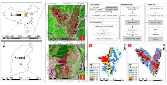
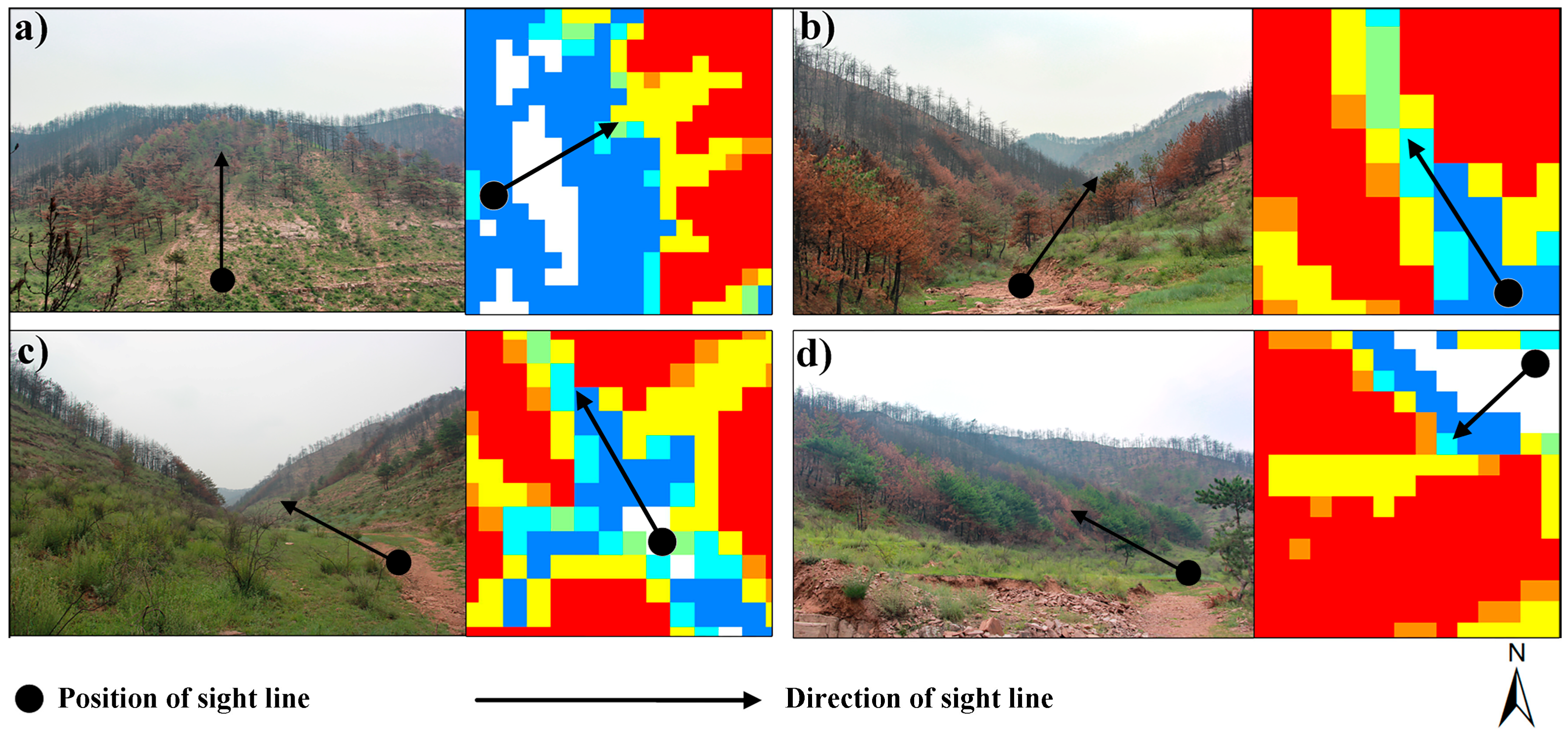
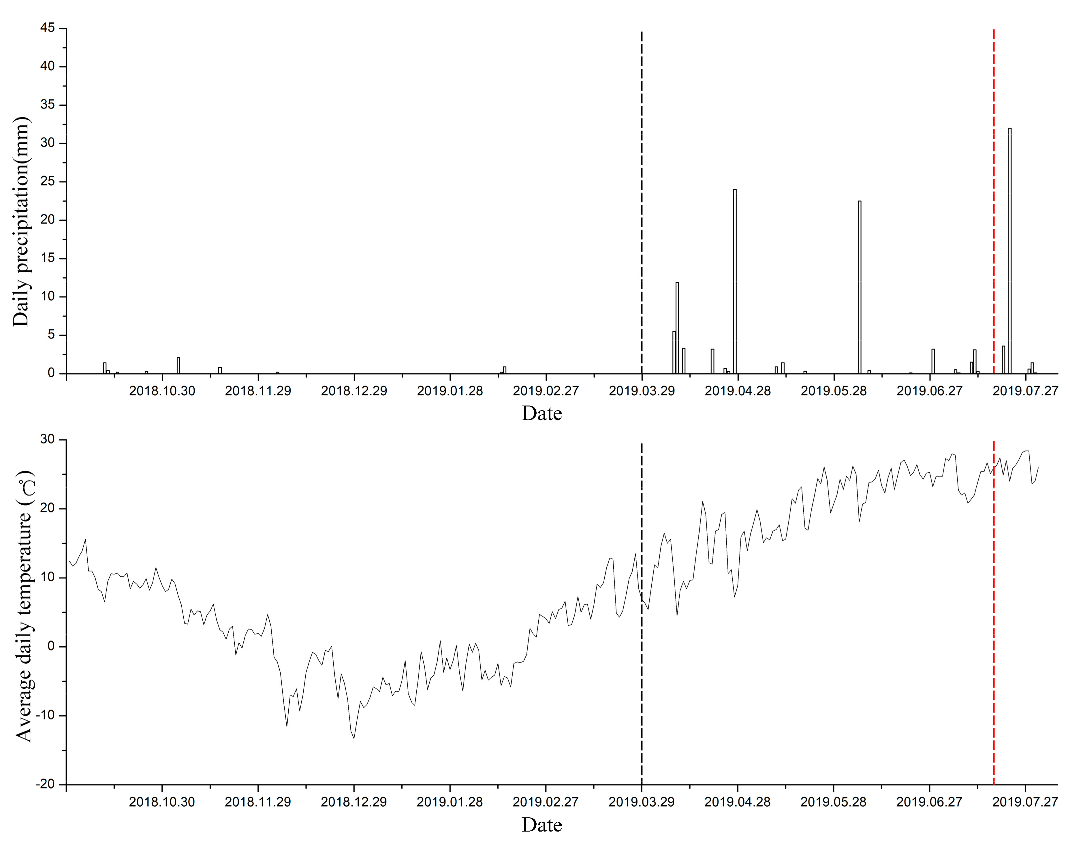
2.1. Study Area

The study area is located at Qinyuan County, central China (111°58′30″E–112°32′30″E, 36°20′20″N–37°00′42″N) (Figure 1). The study area is dominated by overstory vegetation of Pinus tabuliformis while the middle vegetation layer is dominated by low Quercus acutissima and Rosa xanthine and the grass over the soil surface are dominated by Gramineous weeds. Under the management of the local government’s policy of closing hills for reforestation, the vegetation growth in the study area is very dense, and the TCC in most areas is more than 50%. The height of Pinus tabulaeformis in the study area ranged from 3 to 5 m, which has a positive correlation with fire behavior [32]. Pinus tabulaeformis will become very flammable in dry and hot weather for a long time. At the same time, pine balls will help the fire spread faster with the help of wind. The topography of the study area is rugged, and the altitudes range from 1020 to 1639 m. The average annual rainfall in this region is 656.7 mm. The average annual relative humidity is 65% and the average annual temperature is 8.7 °C. Maximum and minimum precipitations were recorded in July–September and November–March, respectively. From November to March there is little precipitation, and the temperature will continue to rise from about −10 °C to 15 °C. During this period, sparse precipitation and temperature rise will help forest ecosystems accumulate large amounts of dry and flammable fuels. Generally, the fire season begins in March and ends in May.

2.2. Data Collection

In March 2019, two fires that caught the attention nationwide broke out in south (fire 1, 14 March) and north of (fire 2, 29 March) Qinyuan County (Figure 1). Fire 1 was small in scale (approximately burnt 48 ha), but six firefighters died during fire suppression because of sudden changes in wind direction. There were no casualties in fire 2 even though the burn area was larger (approximately 16,788 ha,). The post-fire field survey was conducted from 18 to 23 July 2019. The CBI was measured based on the field criterion proposed by Key and Benson (2006) and used as the ground truth to validate the accuracy of burn severity estimated by the methodology proposed in this study. There was a total of 20 and 143 field CBIs recorded for fire 1 and fire 2, respectively (Figure 1). Field plots were selected within areas with homogeneous burn severity levels, as recommended by Key and Benson [7].

2.3. Remote Sensing Data

2.3.1. Sentinel-2A MSI Data

In this study, the Sentinel-2A Multi-Spectral Instrument (MSI) data were used as the satellite data source to estimate burn severity. The Sentinel-2A MSI data has 13 spectral channels in the visible (VIS), near-infrared (NIR), and shortwave infrared (SWIR) spectral ranges. To keep the spatial resolution (20 m) consistency of surface reflectance data, nine out of the 13 spectral bands (bands 2–7, 8a, 11, and 12) were used to estimate burn severity (Table 1). Considering that NBR can provide more additional spectral information, the post-fire NBR, normalized of bands 8a and 12 were also used for burn severity estimation. To ensure that it is closest to the field survey time, the post-fire imagery was acquired on 30th June 2019. This image is the closest to the sampling date and has the best imaging quality. The Sentinel-2A MSI Level-1C data used in this study were downloaded from the Copernicus Open Access Hub (https://scihub.copernicus.eu/). The atmospheric correction of Sentinel-2A MSI data was conducted by use of the Sen2Cor Tool (version 2.3.1) [33,34]. The reflectance of the Level-1C Bottom-of-Atmosphere (BOA) was converted to Level-2A by using the default parameters. Sen2Cor consists of two main modules: the Scene Classification (SCL) module and the Atmospheric Correction (AC) module [35]. The AC is executed using a set of Look Up Tables (LUTs) generated by libRadtran [36]. AC includes three configuration parameters: aerosol type, atmosphere type, and ozone content. The aerosol type can be set as rural or maritime (the default setting is rural). There are two atmosphere types (mid-latitude summer or mid-latitude winter) that can be set, which will be automatically selected by Sen2Cor according to the geographic location and climatology of the scene [35]. The Ozone content is also automatically selected by Sen2Cor according to the geographic location and climatology.

2.3.2. Landsat Vegetation Continuous Fields Product

The Landsat Vegetation Continuous Fields (VCF) tree cover product contains estimates of the TCC in each 30 m pixel covered by woody vegetation greater than 5 m in height [37]. The product extracts all seven bands of Landsat 5 Thematic Mapper (TM) and/or Landsat 7 Enhanced Thematic Mapper Plus (ETM+) by rescaling the 250 m Moderate-resolution Imaging Spectroradiometer (MODIS) Vegetation Continuous Fields (VCF) Tree Cover layer. On 5 March 2019, the NASA Land Cover/Land Use Change Program released version 4 of the Global 30 m Landsat tree canopy cover product. The fourth edition of the TCC product replaced the previous version of global tree canopy cover estimates for 2000, 2005, 2010, and 2015. Previous versions of TCC were collected using the Landsat Global Land Survey, but version 4 was created by mining and processing entire Landsat archives, providing improved and accurate representation for specific years (https://landsat.gsfc.nasa.gov/global-30m-landsat-tree-canopy-version-4-released/). In this study, the TCC layer of 2015 was used to parameterize and constrain the RTM. The forests in the study area are natural forests with little human intervention, and there has been no forest fire in the study area since 2015, thus the TCC layer in 2015 can be used to represent the situation before the fire. For more information about this dataset please visit http://landcover.org/data/landsatTreecover. The TCC layer of Landsat VCF data was resampled to 20 m matching the spatial resolution of Sentinel-2A MSI data using nearest-neighbor interpolation.

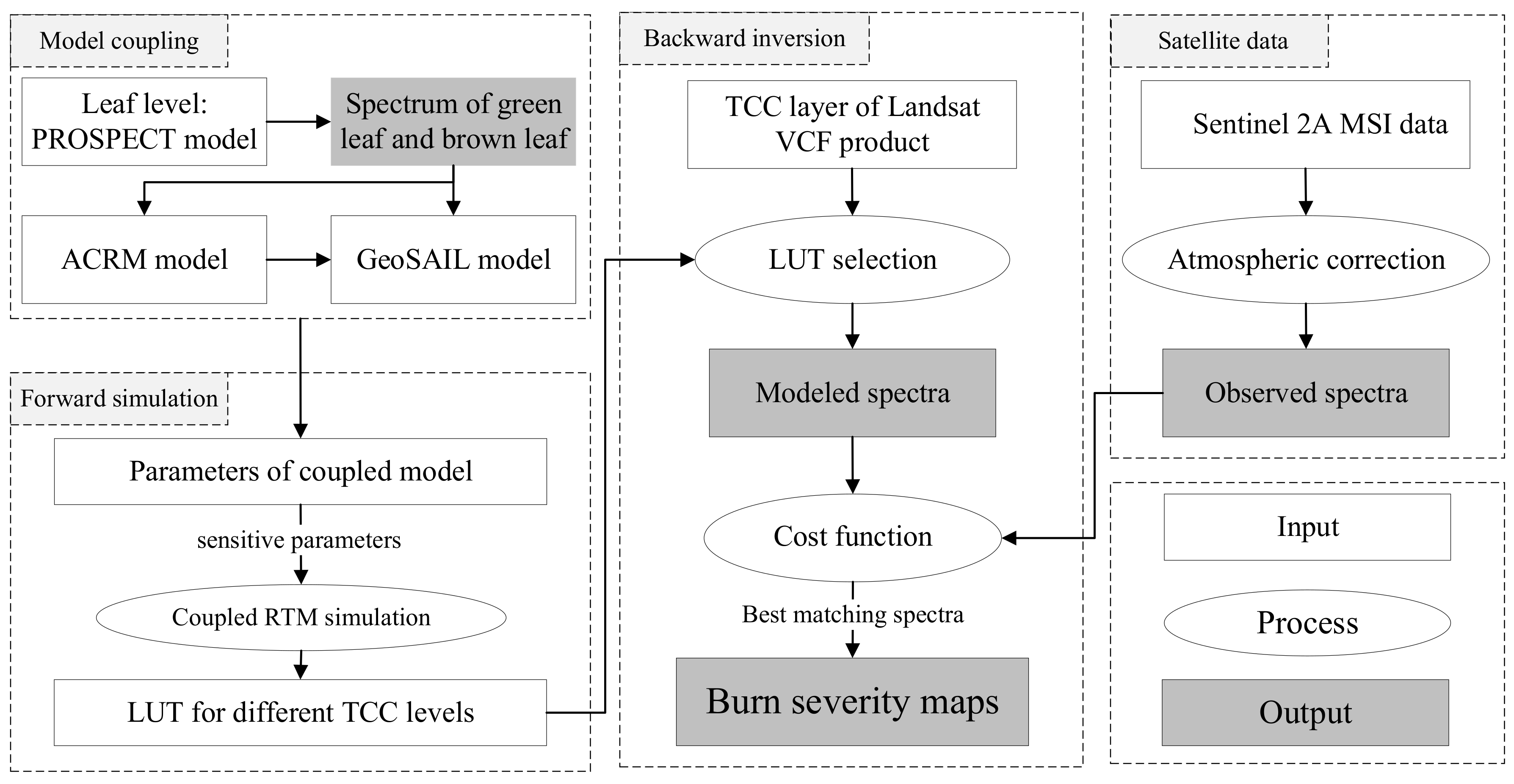
2.4. Burn Severity Retrieval Using Coupled RTM

The methodology to retrieve burn severity using coupled RTM is carried out in four steps (Figure 2): (i) remote sensing data preprocessing, including the atmospheric correction of the Sentinel 2A MSI data and resampling of the Landsat VCF product; (ii) couple RTMs of leaf and canopy level for burn severity retrieval; (iii) forward modeling, including the parameterization of the coupled RTM based on the sensitivity analysis results of previous studies and construction of the LUT [24]; and (iv) Coupled RTM backward inversion procedure by finding the simulated surface reflectance (saved in the LUT) that most similar to the extracted spectrum from satellite remotely sensed data by use of a cost function [38]. The coupled RTM can simulate the radiative transfer characteristics of three-layer vegetation and has greater potential to accurately estimate burn severity worldwide given it directly accounts for variation in TCC to avoid misclassify burn severity without the need of determining a site-specific stand density–TCC relationship.

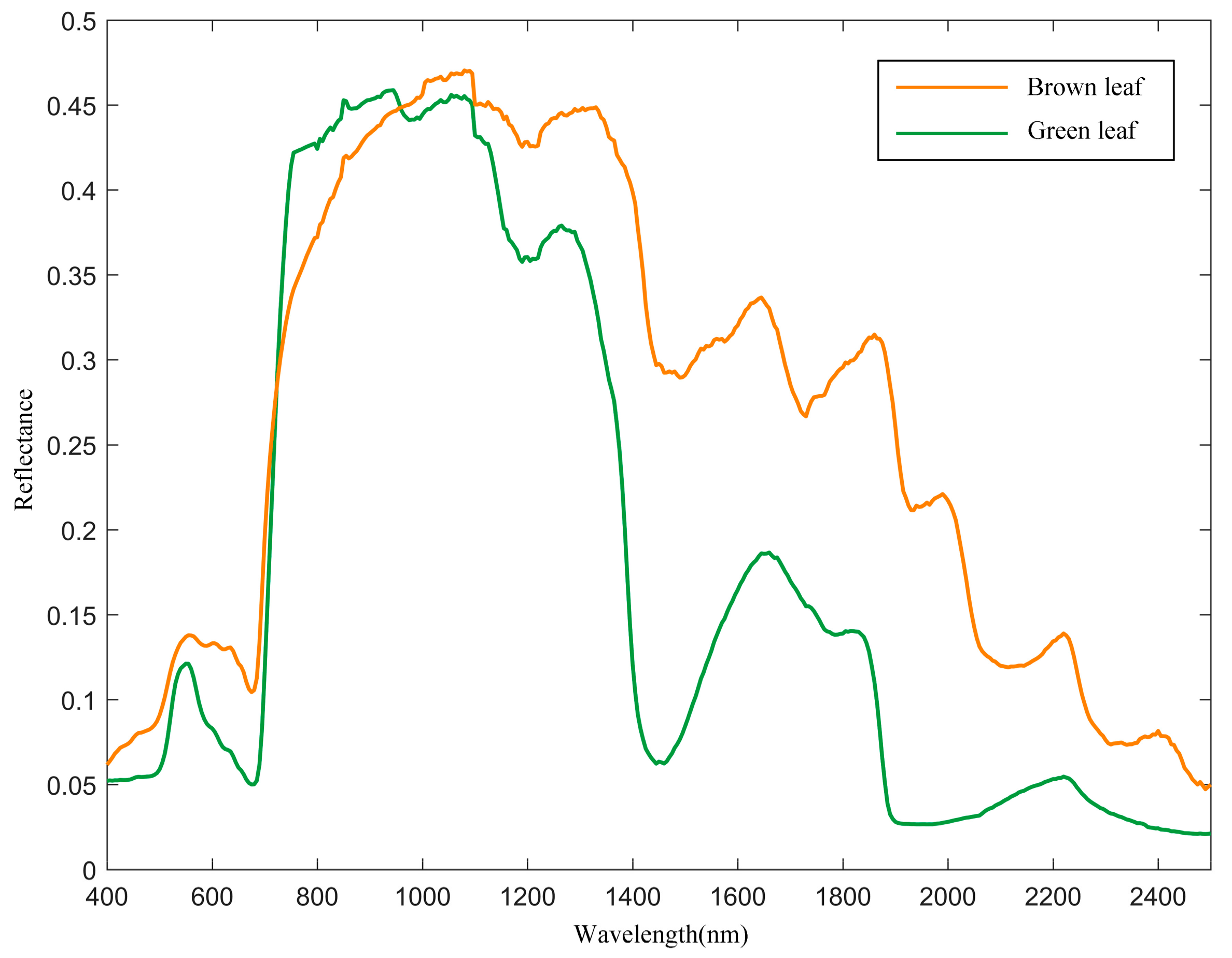
2.4.1. Model Selection and Coupling

Several vegetation layers are considered for CBI evaluation. Therefore, the selected RTM should have the capacity to simulate the spectrum of multi-layered forests. In this study, the leaf-level RTM PROSPECT [39], canopy-level RTM ACRM [40,41], and GeoSail RTM [42] were coupled to simulate the spectra of the multi-layered forests for burn severity retrieval. The coupled RTM has the capacity of simulating the radiative transfer characteristics of three-layer vegetation and has greater potential to accurately estimate burn severity worldwide given it directly accounts for variation in TCC to avoid misclassifying burn severity without the need of determining a site-specific stand density–TCC relationship.
The PROSPECT model was used to simulate the spectrum of a green and brown needle leaf. Although other RTMs may be more suitable for simulating the reflectance and transmittance of needles than PROSPECT (e.g., LIBERTY model proposed by Dawson et al. [43]), they are not as operational as PROSPECT because it requires more input variables with more complex parameters. Besides, PROSPECT has been successfully applied to the simulation of needle leaves’ spectra in many studies [24,44,45]. The PROSPECT model is a leaf optical model, which calculates the reflectance and transmittance of the leaf hemisphere in the range of 400 to 2500 nm in steps of 1 nm. The calculated reflectance and transmittance are expressed as a function of six input parameters: leaf structure parameter, N (unit-less); Cab (μg cm−2); Equivalent Water Thickness, Cw (g cm−2); Dry Matter Content, Cm (g cm−2); carotenoid content, Car (μg cm−2); and leaf brown pigment, Cs (unit-less).
ACRM assumes that the canopy consists of a homogeneous vegetation layer and a thin layer of vegetation on the soil surface. The model is an extension of the homogeneous multispectral canopy reflectance model MSRM [46] and Markov chain canopy reflectance model MCRM [47]. The model has a step size of 1 nm in the 400 to 2400 nm spectral range. This RTM is thus suitable for simulating the spectra of middle and lower canopies. Here, the ACRM was coupled with the GeoSail model by replacing the spectra of the bare soil input of GeoSail and considering the vertical stratification characteristics of vegetation in the study area. The ACRM was used to simulate the spectrum of middle vegetation layers and grass over the soil surface.
The GeoSail model was used to simulate the spectrum of the upper tree canopy layer since it is a geometric model that considers the geometry and shadowing effects of forest stands. The Geosail model described the canopy reflectance of heterogeneous and discontinuous vegetation types with relatively simple input parameters [42] and has been successfully used for burn severity retrieval [24]. The tree coverage parameter FCOV in the GeoSail model can be directly constrained by satellite-derived TCC without proxy parameters such as stand density, therefore the coupled RTM has greater potential than FRT RTM in burn severity retrieval. All the canopy vegetation parameters required by the coupled RTM are listed in Table 2. For the range and default values of model parameters, refer to the user’s guide and previous studies [24,27,30].
For the coupled RTM, the diffuse radiation was set as the dominant radiation for the grassland layer by the hypothesis that most of the direct radiation intercepted by the tree canopy. Therefore, the bi-hemispherical reflectance rather than the BRDF of the understory was modeled in this case. Besides, the spectral reflectance of the background originally in the GeoSail is assumed to be the reflectance of Lambertian while the spectra modeled by the PROSAIL (PROSPECT and Scattering by Arbitrarily Inclined Leaves) is non-Lambertian.

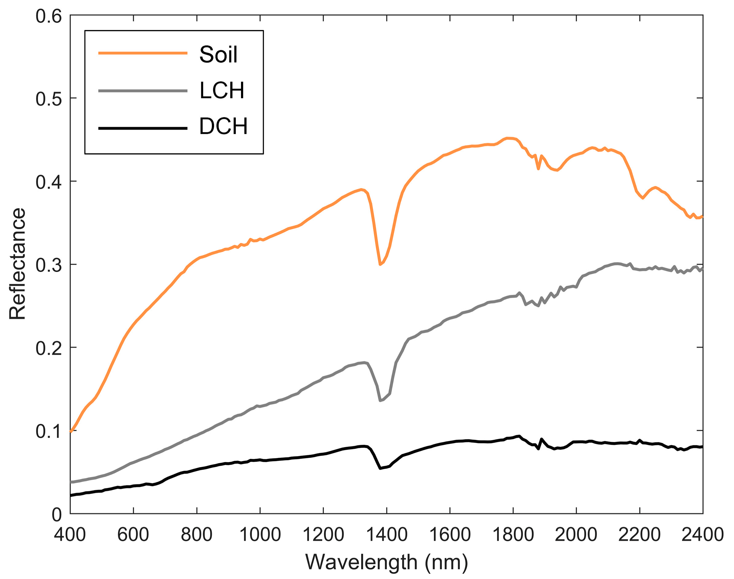
2.4.2. Model Parameterization and Forward Modeling

The parameterization of the coupled RTM was based on prior information obtained from field quantitative measurements, qualitative survey, previous studies [24,30], and Sentinel 2A MSI metadata. Only the parameters most sensitive to the change of the target bands according to previous analysis from De Santis et al. [24] and Yin et al. [9] were used, i.e., the fractional cover (FCOV), leaf area index (LAI), and water content (Cw) are most sensitive to the short-wave infrared (SWIR) band. In detail, the LAI and FCOV are the most sensitive parameters for the NIR band. The Cab, LAI, and brown pigments content (Cs) are the most sensitive parameters for VIS bands. Therefore, the sensitive parameters selected for the GeoSail model were FCOV and LAI at canopy level and Cw, Cab, and Cs at the leaf level, as illustrated in Table 3. In the CBI field criterion, burn severity is evaluated using a set of variables for each vegetation vertical strata, and the CBI increases with the proportion of brown over green leaves. Therefore, the PROSPECT model was used at the leaf level to simulate only one representative spectrum for green and brown reference leaf types. The parameterization for PROSPECT model were N = 2.5, Cab = 70 μg cm−2, Cw = 0.048 g cm−2, and Cs = 0.2 for green leaf [48] while to N = 2.5, Cab = 20 μg cm−2, Cw = 0.008 g cm−2, and Cs = 1.5 for brown leaf [49]. The simulated green and brown leaf spectrum based on the PROSPECT model was shown in Figure 3. The ACRM model was calibrated following Yin et al. [9]. For the middle vegetation layer, the sensitive parameters are LAI of middle vegetation and a series of biochemical parameters determining leaf color (N, Cab, Cw, and Cs); for the lower vegetation layer, the sensitive parameters are LAI of lower vegetation and biochemical parameters determining leaf color (N, Cab, Cw, and Cs) (Table 3).
Considering the uncertainty caused by unrealistic combinations of the input model variables, a supervised simulation scheme was executed to reduce the error because it is better than the full range variations [24,26]. The parameter FCOV (range from 0 to 0.8) in the GeoSail model was set as the only free variable to generate the LUT. When the coupling model is forward simulated, the spectral curves corresponding to different TCC conditions can be generated with the variation of FCOV. A combination example of the model input parameters used to generate LUT is listed in Table 3. The background shortly after wildfires usually consists mainly of soil and charcoal [24]. Therefore, three reference spectra were considered as the background layer for the model input: soil, dark charcoal (DCH), and light charcoal (LCH; a mixture of charcoal and ash) (Figure 4). The soil spectra were measured on sandy soil with moderate moisture, while the spectrum of dark and light charcoal was measured with GER 2600 field spectro-radiometer (Geophysical & Environmental Research Corporation, Millbrook, NY, USA) by De Santis et al. [24]. The simulated CBI value variation from 0.5–3 with steps of 0.1. The burn severity can be divided into low, moderate, and high level by use of CBI threshold values of 2 and 2.5 [9]. For low burn severity level, only the grassland and shrub on the soil surface were burned. For moderate burn severity level, the underlying grass and shrubs were completely burned and the understory of the tree was slightly burned, but the trees still retained the green canopy. For high burn severity level, the low and middle vegetation strata were completely burned and the crown was severely burned. For the part of CBI lower than 2.5, only the DCH scenario was simulated. For the part of CBI higher than 2.5, the organic matter in the soil and all vegetation strata is burned, the substratum can be charcoal or ash, therefore both DCH and LCH scenarios are simulated. Finally, there are 352 combinations of input parameters used to construct the LUT for burn severity retrieval.

2.4.3. Coupled RTM Inversion

In this study, the LUT was used as the inversion algorithm to retrieve burn severity using Sentinel-2A MSI satellite remotely sensed data. We derived burn severity using the information on TCC to constrain the backward inversion procedure. For each pixel in the burnt area, the Landsat VCF product was served to select the corresponding LUT. The model simulated spectral reflectance in the LUT corresponding to a specific TCC range was subsequently compared to the extracted surface reflectance of the pixel by use of a cost function. The Spectral Angle Mapper (SAM) was used as the cost function to find the model simulated spectral reflectance that was most similar to the spectra reflectance extracted from remotely sensed data. SAM is a supervised classification technology based on pixels. SAM solves spectral similarity by calculating the spectral angle (SA) between two spectral vectors [50,51]. This angle is independent of the length of vectors and is therefore insensitive to the illumination or albedo effects (Equation (1)). Consequently, SAM can eliminate most of the errors introduced by terrain relief [23].
SA = cos 1 i = 1 n b t i r i i = 1 n b t i 2 1 2 i = 1 n b r i 2 1 2
The i represents the band number, nb represents the number of the bands, and t and r represent the simulated and observed spectrum, respectively. SA between the simulated and observed reflectance was calculated as the cost function to estimate the biophysical and biochemical variables of the vegetation that corresponding to certain CBI values. The R square (R2), root mean square error (RMSE), and slope between the measured and estimated CBI were used as the accuracy evaluation index. The backward inversion process in this study was executed by use of all nine Sentinel-2A MSI bands and the coupled RTM with TCC constraint (labeled as CP-RTM+TCC). In addition to the nine spectral bands of Sentinel-2A MSI data mentioned above, the post-fire NBR was also used as an additional vector to provide more spectral information and improve the accuracy of burn severity retrieval.

2.4.4. Methodological Comparison

To compare and evaluate the merit of our proposed method (labeled as CP-RTM+TCC), we derived burn severity using three other existing methods. In the first method, the coupled RTM is inverted using a global optimal search and without TCC constraint (labeled as CP-RTM+GOS). The second one is the method used by Yin et al. [9] (labeled as FRT+TCC). In this method, the burn severity was estimated using the FRT model with TCC constraint. The third method uses a random forest (RF) algorithm. The RF classifier is particularly useful for burn severity mapping with promising accuracy [18,19,52]. In the RF method, the independent variables are the nine spectral bands and the post-fire NBR index of Sentinel 2A MSI data, and the dependent variable is CBI. First, the field measured plots were randomly divided into three samples (each sample comprised about 54 CBI measurements). Second, two samples (i.e., the training sample) were used for RF model calibration, and the other sample (i.e., the testing sample) was used for the validation. Third, the process was repeated three times to adequately test the performance of the RF method [53]. To minimize the statistical error caused by each run of the RT model, we set the number of trees to 1000 and run 100 times to train each RF model.

3. Results

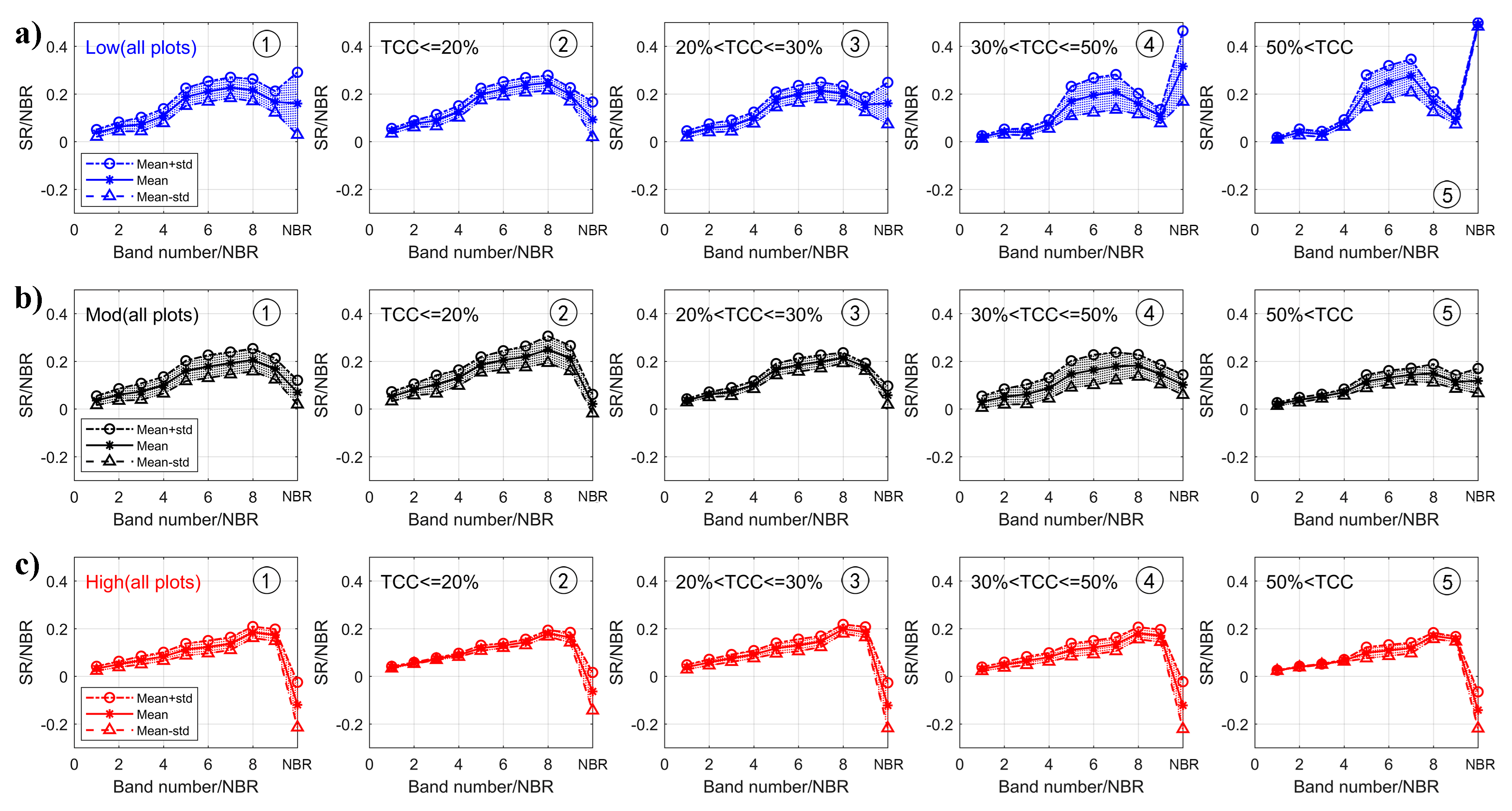
3.1. Influence of TCC on the Spectral Response of Burn Severity

The surface reflectance and post-fire NBR of all the field plots were extracted from Sentinel-2A MSI data from locations corresponding to our sampling locations and averaged by burn severity level and TCC (<20%, 20%–30%, 30%–50%, and >50%) to prove the influence of TCC on the spectral response and the confusion between different burn severity levels (Figure 5). Under this circumstance, the burn severity was divided into low, moderate, and high level by use of CBI threshold values of 2 and 2.5 [9]. Figure 5(a1,b1), and Figure 5(c1) represent the extracted mean reflectance from all field plots without constraining TCC. The averaged reflectance of all field plots obscured the reflectance variation between different TCC ranges. By analyzing the spectrum of three different levels of burn severity under different TCC, it can be found that the high-level burn severity is not sensitive to the change of tree coverage, while the medium level burn severity shows little sensitivity to the change of tree coverage, and the low-level burn severity is most sensitive to the change of tree coverage. This was also observed from the spectral angle (SA) between the spectra of lowest and highest TCC within the same burn severity. The SA was 0.68 (Figure 5(a2,a5)), 0.33 (Figure 5(b2,b5)), and 0.27 (Figure 5(c1,c5)) for low, moderate, and high burn severity, respectively. For TCC over 50%, the spectral characteristic of the high burn severity exhibited similar characteristics to the moderate and low burn severity with the lower TCC. For a detailed analysis of the influence of TCC on the inversion of burn severity, please refer to Yin et al. [9]. The results given in Figure 5 indicate that if the TCC is not considered in the inversion of burn severity, spectral confusion will be caused by the change of TCC between different burn severity levels.

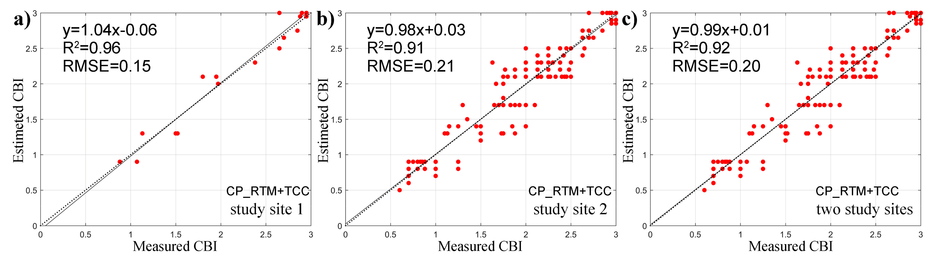
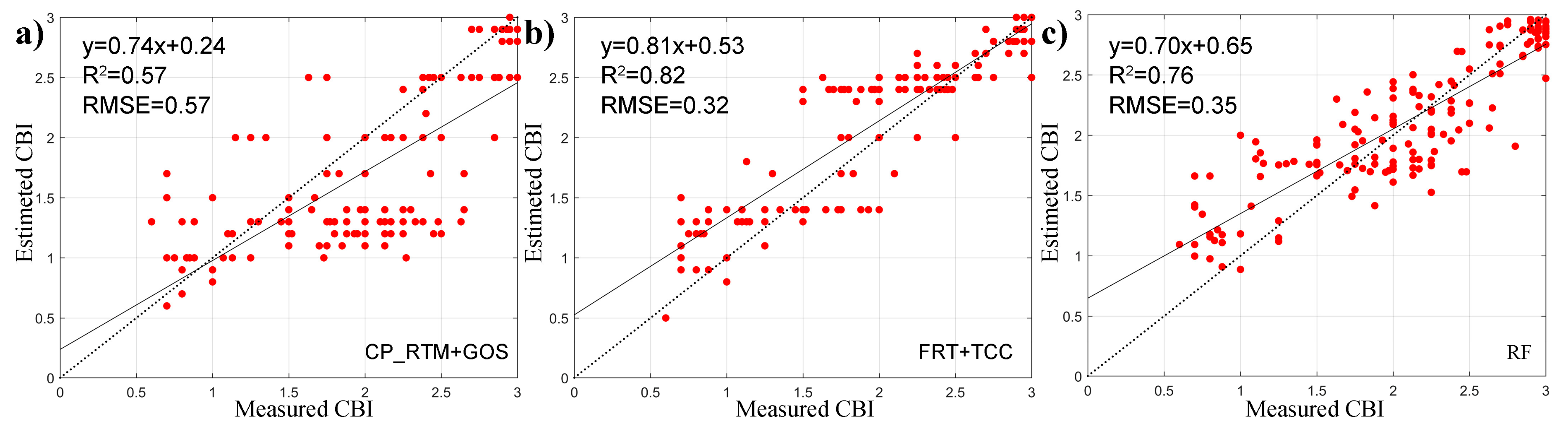
3.2. Evaluation of Burn Severity Estimates

A total of 163 CBI values recorded at two sample sites were used to validate the retrieved CBI. The CBI was estimated based on the coupled RTM constrained by TCC information provided by satellite estimates (CP_RTM+TCC). The validation results at both sites showed a high correlation between the observed and simulated CBI (R2 equal to 0.96 for study site 1 (Figure 6a), 0.91 for study site 2 (Figure 6b), and 0.92 for two study sites (Figure 6c)) and an almost 1:1 linear fit (slope: ~1; constant: ~0). The RMSE is also very low (0.15 for study site 1, 0.21 for study site 2, and 0.20 for two study sites).
When comparing the method proposed in this study with the burn severity estimations obtained with CP_RTM+GOS, FRT+TCC, and RF methods (Table 4 and Figure 7), the method proposed in this study but without TCC constrains (CP_ RTM+GOS method) presents slightly worse performance than FRT+TCC and RF. Figure 7b also shows that the estimated results of the FRT+TCC method yield a relatively higher accuracy (R2 equal to 0.82, RMSE equal to 0.32, and slope equal to 0.81). As can be indicated from Figure 7c that the validation accuracy (R2 = 0.76, RMSE = o 0.35 and slop = 0.7) based on the RF method is higher than CP_RTM+GOS but lower that of the FRT+TCC method. Overall, the CP_RTM+TCC method (Figure 6) performed best (R2 equal to 0.92, RMSE equal to 0.2 and slop equal to 0.99) among these four methods.

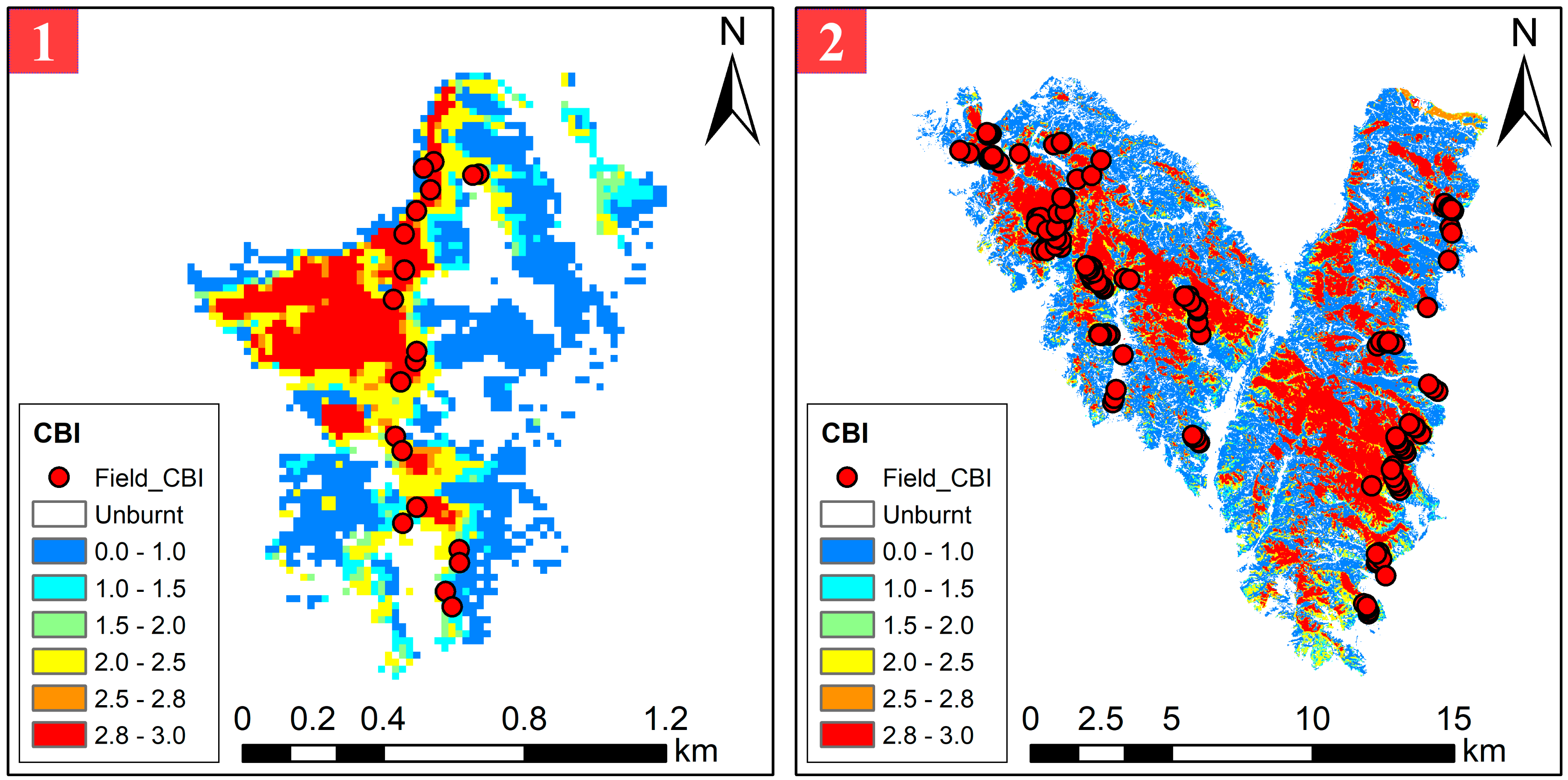
3.3. Burn Severity Mapping

The focus of this study is burn severity estimation, so the dNBR as well as visual interpretation were used to extract burn area. Burn severity maps for the two sample sites of Qinyuan country were produced based on the burn area extraction and the CP_RTM+TCC method (Figure 8). The high-level burn severity range (CBI ≥ 2.5) in site 1 is mainly distributed in the western area because the elevation of the western area of the site is relatively high and its main vegetation type is dense and dry Pinus tabulaeformis forest, which is quite flammable. The eastern part corresponds to the foot and hillside with relatively low elevation, the vegetation types are mainly yellow rose, low bush, and dense herbaceous vegetation, and the burn severity type is mainly of medium (2 ≤ CBI < 2.5) and low level (CBI < 2). For study site 2, the main vegetation type is also Pinus tabulaeformis. The middle and high-level burn severity are mainly distributed at the top of the mountain with relatively high altitude, while the low-level burn severity is mainly distributed at the foot of the mountain with relatively low and flat terrain. From the spatial distribution map of burn severity in study area 2, we can also see that there are more areas with CBI over 2.8 and below 2.0, but fewer areas with CBI between 2.0 and 2.8 than in study site 1.
In the field measurement, in addition to the photos used to estimate the CBI value of the sample plots, we also selected some areas with a wide view to take panoramic photos for quantitative verification of burn severity inversion results. The qualitative validation was carried out by comparing the field landscape panoramic photos and the spatial distribution map of burn severity (Figure 9). A total of four validation points were selected: two (Figure 9b,c) of them point to the valley, and the other two (Figure 9a,d) point to the hillside. The qualitative accuracy validation results indicated that the burn severity map and the landscape panoramic photos from the field survey showed good spatial distribution consistency. This provided further evidence for the reliability of our burn severity estimates.

4. Discussion

In this study, the burn severity of two forest fires was estimated using a coupled RTM and Sentinel-2A MSI reflectance data. ACRM assumes that the canopy consists of a homogeneous vegetation layer and a thin layer of vegetation on the soil surface, which is thus suitable for simulating the spectra of middle and lower canopies. The GeoSail model is a geometric model that considers the geometry and shadowing effects of forest stands and was used to simulate the spectrum of the upper tree canopy layer. The ACRM was coupled with the GeoSail model by replacing the spectra of the bare soil input of GeoSail and considering the vertical stratification characteristics of vegetation in the study area. The coupled RTM can simulate the radiative transfer characteristics of three-layer vegetation and has greater potential to accurately estimate burn severity worldwide given it directly accounts for variation in TCC to avoid misclassify burn severity without the need of determining a site-specific stand density–TCC relationship.
Compared with the three existing methods in other studies, the proposed method (CP_ RTM+TCC) in this study performed best. The CP_ RTM+GOS method performed worst because if TCC is not constrained, there is serious spectral confusion between the different burn severity levels. This is similar to the conclusion of Yin et al. [9], who found spectral confusion between different burn severity levels when the influence of TCC was not considered in the RTM forward and backward inversion procedure. Accuracy comparison results also showed that the FRT+TCC method yields a relatively higher accuracy. This is because the influence of tree canopy cover is considered in the FRT+TCC method. However, the accuracy was still lower than that of this study. This is because the stand density was used as a proxy parameter to constrain the TCC in the FRT+TCC method, but stand density is not the only determining parameter of tree coverage. Furthermore, the statistical correlation between stand density and the lack of universality in TCC occurs because the empirical correlation has not been validated other than the Yatir forest in Israel. Therefore, the indirect constraint of tree canopy cover through stand density will produce matching errors, which will affect the estimation accuracy of CBI. In essence, the RF algorithm estimates the burn severity according to the characteristics of spectral reflectance, so it cannot get rid of the influence of TCC. Therefore, the estimated accuracy based on the RF method is still lower than the method proposed in this study.
The spatial distribution of burn severity in the two study sites shows obvious boundary characteristics. Most regions have CBI values above 2.8 or below 2.0, but few regions between 2.0 and 2.8. Combined with field sampling, we analyzed two main reasons for this phenomenon. First, the interval between the fire and the field sampling was nearly 4 months and there was rainfall during this period. The vegetation recovery ability in the low and medium burn severity area was stronger than that in the high burn severity area. Most of the trees are burned completely under the high burn severity level, which hinders quick recovery, and the low and medium burn severity is only affected by the medium degree, supporting recovery faster speeds, which is consistent with the conclusion of Meng et al. [54]. On the other hand, the relationship between vegetation recovery rate after the fire and burn severity is not linear, but is a saddle curve [54]. This curve shows that the forest has certain fire resistance. For example, some trees under fire stress have a short-term loss of canopy leaves but do not die. Therefore, their canopies will recover in a short time after the fire. However, with the increase of forest burn severity, tree survival will decrease as canopies cannot recover from the damage. The areas affected by a moderate burn severity did not cause fatal damage to trees, therefore the recovery rate was the fastest, with quick recovery to the state of lower burn severity level after the fire. In most cases, the damage to trees caused by high burn severity is irreversible, implying slow recovery. Second, field sampling saw that the high burn severity level was mainly distributed in areas with high altitude and high slope. During the period from the fire (29 March) to the field sampling (18 July), there were several precipitation events (>83 mm), and the temperature continued to rise (from 6.9 to 26.3 °C) (Figure 10); this created good conditions for the post-fire recovery of vegetation in the study area. However, because of the fire-related decrease of water storage capacity in mountain forests, there was a slower recovery rate of trees at the top of mountains and in steep areas compared to valleys and relatively flat terrain. In the process of field survey, we also found that the spatial distribution of burn severity has a high correlation with terrain characteristics. For example, the areas with high burn severity are mostly distributed on the top of the mountain and steep hillside, which indicates that terrain factor is the important drive factor of burn severity. Future work will be focus on analyzing the relationship between post-fire burn severity and pre-fire environmental drive factors.
The meteorological data before the forest fire 2 in Qinyuan county were also analyzed. Figure 10 gives the daily average temperature and precipitation data of Taiyuan meteorological station nearest to Qinyuan county (longitude: 112.35°E, latitude: 37.37°N) from 1 October 2018 to 31 July 2019. There was almost no precipitation in the six months before the fire and the temperature continued to rise in the three months before the fire, which provided sufficient external conditions for the fire. This is also evident in the driving effect of meteorological factors on fire. Furthermore, due to the local policy of closing the mountain for forest cultivation, many areas in sample site 2 were completely closed, resulting in the accumulation of a large number of fuel load, including live fuel, such as Pinus tabulaeformis and other shrubs; herbaceous vegetation; and dead fuel represented by litter and humus on the ground. The accumulation of fuel load is also one of the important causes of fire ignition. Meteorological variables are one of the most important factors affecting post-fire vegetation regeneration. Vegetation regeneration and growth are generally highly depending on favorable postfire meteorological conditions, such as conditions with higher moisture and proper temperature [55]. The several precipitation events and the average daily temperature continued to rise in the study area after the fire created good conditions for vegetation regeneration.

5. Conclusions

Burn severity is of vital importance for post-fire forest management and will assist in post-fire vegetation regeneration. In this study, the burn severity of two forest fires in Qinyuan was estimated using coupled RTM and Sentinel 2A MSI data. Traditional optical satellite remotely sensed data-based methods that do not take the variation in TCC into account will lead to spectral confusion in burn severity retrieval. Yin et al. [9] significantly improved the CBI estimation accuracy by using prior TCC information into the forward simulations and backward inversions via the stand density parameter of the FRT model. However, TCC is not only determined by stand density but also canopy diameter. Moreover, the correlation between stand density and TCC is not universal, limiting the application of FRT RTM-based inversion for forest burn severity somewhere else. In this study, ACRM was coupled with the GeoSail model, by replacing the spectra of the bare soil input of GeoSail and considering the vertical stratification characteristics of vegetation in the study area. The tree coverage parameter FCOV in the GeoSail model was directly constrained by TCC without proxy parameters, and therefore has greater potential to accurately estimate burn severity worldwide. The verification of the accuracy of results using four methods (CP_RTM+TCC, CP_RTM+GOS, FRT+TCC, and RF) showed that the method proposed in this study (CP_RTM+TCC) has the highest burn severity estimation accuracy. The more accurate estimation of the burn severity obtained from the approach presented in this study will help land managers to better understand post-fire vegetation regeneration and help in post-fire forest management. Now that a new method for accurately estimate fire severity has been found, future work will be focus on analyzing the relationship between post-fire burn severity and pre-fire environmental drive factors.

Author Contributions

B.H. and X.Q. supervised and fund this research; C.Y., X.Q., and B.H. conceived and designed the experiments; C.Y. performed the experiments and analyzed the data; C.Y. and X.Q. wrote the first version of the manuscript; M.Y. refined the methodology and contributed to the final version of the manuscript; G.L. edited the manuscript. All authors have read and agreed to the published version of the manuscript.

Funding

This work was supported by the National Natural Science Foundation of China (Contract No. 41671361, 41601373, and 41801272) and the Fundamental Research Fund for the Central Universities (Contract No. ZYGX2017KYQD195).

Acknowledgments

We would like to especially thank De Santis who provided the field-measured reflectance of soil, dark charcoal, and light charcoal. The authors are grateful to Long Wang and Lin Chen for their assistance during the field campaigns.

Conflicts of Interest

The authors declare no conflict of interest.

References

  1. Bonan, G.B. Forests and Climate Change: Forcings, Feedbacks, and the Climate Benefits of Forests. Science 2008, 320, 1444–1449. [Google Scholar] [CrossRef] [PubMed] [Green Version]
  2. Liu, Z.; Ballantyne, A.P.; Cooper, L.A. Biophysical feedback of global forest fires on surface temperature. Nat. Commun. 2019, 10, 1–9. [Google Scholar] [CrossRef] [PubMed] [Green Version]
  3. Trumbore, S.; Brando, P.; Hartmann, H. Forest health and global change. Science 2015, 349, 814–818. [Google Scholar] [CrossRef] [PubMed] [Green Version]
  4. Chuvieco, E.; Riaño, D.; Danson, F.M.; Martín, M.P. Use of a radiative transfer model to simulate the postfire spectral response to burn severity. J. Geophys. Res. Space Phys. 2006, 111, 111. [Google Scholar] [CrossRef] [Green Version]
  5. Edwards, A.C.; Russell-Smith, J.; Maier, S.W. A comparison and validation of satellite-derived fire severity mapping techniques in fire prone north Australian savannas: Extreme fires and tree stem mortality. Remote Sens. Environ. 2018, 206, 287–299. [Google Scholar] [CrossRef]
  6. Frolking, S.; Palace, M.W.; Clark, D.B.; Chambers, J.Q.; Shugart, H.H.; Hurtt, G.C. Forest disturbance and recovery: A general review in the context of spaceborne remote sensing of impacts on aboveground biomass and canopy structure. J. Geophys. Res. Space Phys. 2009, 114, 114. [Google Scholar] [CrossRef]
  7. Key, C.; Benson, N. Landscape assessment: Ground measure of severity, the Composite Burn Index. In FIREMON: Fire Effects Monitoring and Inventory System; Lutes, D.C., Ed.; USDA Forest Service, Rocky Mountain Research Station: Fort Collins, CO, USA, 2006; pp. LA8–LA15. [Google Scholar]
  8. De Santis, A.; Chuvieco, E. GeoCBI: A modified version of the Composite Burn Index for the initial assessment of the short-term burn severity from remotely sensed data. Remote Sens. Environ. 2009, 113, 554–562. [Google Scholar] [CrossRef]
  9. Yin, C.; He, B.; Yebra, M.; Quan, X.; Edwards, A.C.; Liu, X.; Liao, Z. Improving burn severity retrieval by integrating tree canopy cover into radiative transfer model simulation. Remote Sens. Environ. 2020, 236, 111454. [Google Scholar] [CrossRef]
  10. Edwards, A.; Maier, S.W.; Hutley, L.B.; Williams, R.J.; Russell-Smith, J. Spectral analysis of fire severity in north Australian tropical savannas. Remote Sens. Environ. 2013, 136, 56–65. [Google Scholar] [CrossRef]
  11. Chuvieco, E. Earth Observation of Wildland Fires in Mediterranean Ecosystems; Springer: Berlin/Heidelberg, Germany, 2009. [Google Scholar]
  12. Miller, J.D.; Knapp, E.E.; Key, C.H.; Skinner, C.; Isbell, C.J.; Creasy, R.M.; Sherlock, J.W. Calibration and validation of the relative differenced Normalized Burn Ratio (RdNBR) to three measures of fire severity in the Sierra Nevada and Klamath Mountains, California, USA. Remote Sens. Environ. 2009, 113, 645–656. [Google Scholar] [CrossRef]
  13. Miller, J.D.; Thode, A.E. Quantifying burn severity in a heterogeneous landscape with a relative version of the delta Normalized Burn Ratio (dNBR). Remote Sens. Environ. 2007, 109, 66–80. [Google Scholar] [CrossRef]
  14. Roy, D.; Boschetti, L.; Trigg, S.N. Remote Sensing of Fire Severity: Assessing the Performance of the Normalized Burn Ratio. IEEE Geosci. Remote Sens. Lett. 2006, 3, 112–116. [Google Scholar] [CrossRef] [Green Version]
  15. Fernández-Manso, O.; Quintano, C.; Fernández-Manso, A. Combining spectral mixture analysis and object-based classification for fire severity mapping. For. Syst. 2009, 18, 296. [Google Scholar] [CrossRef]
  16. Quintano, C.; Fernández-Manso, A.; Roberts, D.A. Multiple Endmember Spectral Mixture Analysis (MESMA) to map burn severity levels from Landsat images in Mediterranean countries. Remote Sens. Environ. 2013, 136, 76–88. [Google Scholar] [CrossRef]
  17. Quintano, C.; Fernández-Manso, A.; Roberts, D.A. Burn severity mapping from Landsat MESMA fraction images and Land Surface Temperature. Remote Sens. Environ. 2017, 190, 83–95. [Google Scholar] [CrossRef]
  18. Collins, L.; Griffioen, P.; Newell, G.; Mellor, A. The utility of Random Forests for wildfire severity mapping. Remote Sens. Environ. 2018, 216, 374–384. [Google Scholar] [CrossRef]
  19. Collins, L.; McCarthy, G.; Mellor, A.; Newell, G.; Smith, L. Training data requirements for fire severity mapping using Landsat imagery and random forest. Remote Sens. Environ. 2020, 245, 111839. [Google Scholar] [CrossRef]
  20. Meddens, A.J.; Kolden, C.A.; Lutz, J.A. Detecting unburned areas within wildfire perimeters using Landsat and ancillary data across the northwestern United States. Remote Sens. Environ. 2016, 186, 275–285. [Google Scholar] [CrossRef]
  21. Ramo, R.; Chuvieco, E. Developing a Random Forest Algorithm for MODIS Global Burned Area Classification. Remote Sens. 2017, 9, 1193. [Google Scholar] [CrossRef] [Green Version]
  22. Hultquist, C.; Chen, G.; Zhao, K. A comparison of Gaussian process regression, random forests and support vector regression for burn severity assessment in diseased forests. Remote Sens. Lett. 2014, 5, 723–732. [Google Scholar] [CrossRef]
  23. De Santis, A.; Chuvieco, E. Burn severity estimation from remotely sensed data: Performance of simulation versus empirical models. Remote Sens. Environ. 2007, 108, 422–435. [Google Scholar] [CrossRef]
  24. De Santis, A.; Chuvieco, E.; Vaughan, P.J. Short-term assessment of burn severity using the inversion of PROSPECT and GeoSail models. Remote Sens. Environ. 2009, 113, 126–136. [Google Scholar] [CrossRef]
  25. De Santis, A.; Asner, G.P.; Vaughan, P.J.; Knapp, D.E. Mapping burn severity and burning efficiency in California using simulation models and Landsat imagery. Remote Sens. Environ. 2010, 114, 1535–1545. [Google Scholar] [CrossRef]
  26. Chuvieco, E.; De Santis, A.; Riaño, D.; Halligan, K. Simulation Approaches for Burn Severity Estimation Using Remotely Sensed Images. Fire Ecol. 2007, 3, 129–150. [Google Scholar] [CrossRef]
  27. Kuusk, A.; Nilson, T. Forest reflectance and transmittance FRT user guide. Sci. Chin. D 2002, 41, 580–586. [Google Scholar]
  28. Kuusk, A.; Kuusk, J.; Lang, M. Modeling directional forest reflectance with the hybrid type forest reflectance model FRT. Remote Sens. Environ. 2014, 149, 196–204. [Google Scholar] [CrossRef]
  29. Kuusk, A.; Nilson, T.; Paas, M.; Lang, M.; Kuusk, J. Validation of the forest radiative transfer model FRT. Remote Sens. Environ. 2008, 112, 51–58. [Google Scholar] [CrossRef]
  30. Quan, X.; He, B.; Yebra, M.; Yin, C.; Liao, Z.; Li, X. Retrieval of forest fuel moisture content using a coupled radiative transfer model. Environ. Model. Softw. 2017, 95, 290–302. [Google Scholar] [CrossRef]
  31. Sprintsin, M.; Karnieli, A.; Sprintsin, S.; Cohen, S.; Berliner, P. Relationships between stand density and canopy structure in a dryland forest as estimated by ground-based measurements and multi-spectral spaceborne images. J. Arid. Environ. 2009, 73, 955–962. [Google Scholar] [CrossRef]
  32. Lianqiang, L.; Shukui, N.; Changsen, T.; Ling, C.; Feng, C. Correlations between stand structure and surface potential fire behavior of Pinus tabuliformis forests in Miaofeng Mountain of Beijing. J. Beijing For. Univ. 2019, 1, 73–81. [Google Scholar] [CrossRef]
  33. Gascon, F.; Bouzinac, C.; Thépaut, O.; Jung, M.; Francesconi, B.; Louis, J.; Lonjou, V.; Lafrance, B.; Massera, S.; Gaudel-Vacaresse, A.; et al. Copernicus Sentinel-2A Calibration and Products Validation Status. Remote Sens. 2017, 9, 584. [Google Scholar] [CrossRef] [Green Version]
  34. Louis, J.; Debaecker, V.; Pflug, B.; Main-Knorn, M.; Bieniarz, J.; Mueller-Wilm, U.; Cadau, E.; Gascon, F. Sentinel-2 Sen2Cor: L2A processor for users. In Proceedings of the Living Planet Symposium 2016, Prague, Czech Republic, 9–13 May 2016; pp. 1–8. [Google Scholar]
  35. Main-Knorn, M.; Pflug, B.; Louis, J.; Debaecker, V.; Müller-Wilms, U.; Gascon, F. Sen2Cor for Sentinel-2. In Proceedings of the Image and Signal Processing for Remote Sensing XXIII, Warsaw, Poland, 11–14 September 2017; p. 1042704. [Google Scholar]
  36. Mayer, B.; Kylling, A. Technical note: The libRadtran software package for radiative transfer calculations—Description and examples of use. Atmos. Chem. Phys. Discuss. 2005, 5, 1855–1877. [Google Scholar] [CrossRef] [Green Version]
  37. Sexton, J.O.; Song, X.-P.; Feng, M.; Noojipady, P.; Anand, A.; Huang, C.; Kim, D.-H.; Collins, K.M.; Channan, S.; DiMiceli, C.; et al. Global, 30-m resolution continuous fields of tree cover: Landsat-based rescaling of MODIS vegetation continuous fields with lidar-based estimates of error. Int. J. Digit. Earth 2013, 6, 427–448. [Google Scholar] [CrossRef] [Green Version]
  38. Yebra, M.; Quan, X.; Riaño, D.; Larraondo, P.R.; Van Dijk, A.I.; Cary, G.J. A fuel moisture content and flammability monitoring methodology for continental Australia based on optical remote sensing. Remote Sens. Environ. 2018, 212, 260–272. [Google Scholar] [CrossRef]
  39. Jacquemoud, S.; Baret, F. PROSPECT: A model of leaf optical properties spectra. Remote Sens. Environ. 1990, 34, 75–91. [Google Scholar] [CrossRef]
  40. Kuusk, A. A Directional Multispectral Forest Reflectance Model. Remote Sens. Environ. 2000, 72, 244–252. [Google Scholar] [CrossRef]
  41. Kuusk, A. A two-layer canopy reflectance model. J. Quant. Spectrosc. Radiat. Transf. 2001, 71, 1–9. [Google Scholar] [CrossRef]
  42. Huemmrich, K.F. The GeoSail model: A simple addition to the SAIL model to describe discontinuous canopy reflectance. Remote Sens. Environ. 2001, 75, 423–431. [Google Scholar] [CrossRef]
  43. Dawson, T.P.; Curran, P.J.; Plummer, S.E. LIBERTY—Modeling the Effects of Leaf Biochemical Concentration on Reflectance Spectra. Remote Sens. Environ. 1998, 65, 50–60. [Google Scholar] [CrossRef]
  44. Cheng, Y.-B.; Zarco-Tejada, P.J.; Riaño, D.; Rueda, C.A.; Ustin, S. Estimating vegetation water content with hyperspectral data for different canopy scenarios: Relationships between AVIRIS and MODIS indexes. Remote Sens. Environ. 2006, 105, 354–366. [Google Scholar] [CrossRef]
  45. Zarco-Tejada, P.J.; Miller, J.R.; Harron, J.; Hu, B.; Noland, T.L.; Goel, N.; Mohammed, G.H.; Sampson, P. Needle chlorophyll content estimation through model inversion using hyperspectral data from boreal conifer forest canopies. Remote Sens. Environ. 2004, 89, 189–199. [Google Scholar] [CrossRef]
  46. Kuusk, A. A multispectral canopy reflectance model. Remote Sens. Environ. 1994, 50, 75–82. [Google Scholar] [CrossRef]
  47. Kuusk, A. A Markov chain model of canopy reflectance. Agric. For. Meteorol. 1995, 76, 221–236. [Google Scholar] [CrossRef]
  48. Kötz, B.; Schaepman, M.; Morsdorf, F.; Bowyer, P.; Itten, K.; Allgöwer, B. Radiative transfer modeling within a heterogeneous canopy for estimation of forest fire fuel properties. Remote Sens. Environ. 2004, 92, 332–344. [Google Scholar] [CrossRef]
  49. Lang, M.; Nilson, T.; Kuusk, A.; Kiviste, A.; Hordo, M. The performance of different leaf mass and crown diameter models in forming the input of a forest reflectance model: A test on forest growth sampleplots and Landsat ETM images. In Proceedings of the ForestSat 2005, Boras, Switzerland, 31 May–3 June 2005. [Google Scholar]
  50. Dennison, P.E.; Halligan, K.Q.; Roberts, D.A. A comparison of error metrics and constraints for multiple endmember spectral mixture analysis and spectral angle mapper. Remote Sens. Environ. 2004, 93, 359–367. [Google Scholar] [CrossRef]
  51. Kruse, F.; Lefkoff, A.; Boardman, J.; Heidebrecht, K.; Shapiro, A.; Barloon, P.; Goetz, A. The spectral image processing system (SIPS)—Interactive visualization and analysis of imaging spectrometer data. Remote Sens. Environ. 1993, 44, 145–163. [Google Scholar] [CrossRef]
  52. Parks, S.A.; Holsinger, L.M.; Koontz, M.J.; Collins, L.; Whitman, E.; Parisien, M.-A.; Loehman, R.; Barnes, J.L.; Bourdon, J.-F.; Boucher, J.; et al. Giving Ecological Meaning to Satellite-Derived Fire Severity Metrics across North American Forests. Remote Sens. 2019, 11, 1735. [Google Scholar] [CrossRef] [Green Version]
  53. Wang, L.; Quan, X.; He, B.; Yebra, M.; Xing, M.; Liu, X. Assessment of the Dual Polarimetric Sentinel-1A Data for Forest Fuel Moisture Content Estimation. Remote Sens. 2019, 11, 1568. [Google Scholar] [CrossRef] [Green Version]
  54. Meng, R.; Wu, J.; Zhao, F.; Cook, B.D.; Hanavan, R.P.; Serbin, S.P. Measuring short-term post-fire forest recovery across a burn severity gradient in a mixed pine-oak forest using multi-sensor remote sensing techniques. Remote Sens. Environ. 2018, 210, 282–296. [Google Scholar] [CrossRef]
  55. Liu, Z. Effects of climate and fire on short-term vegetation recovery in the boreal larch forests of Northeastern China. Sci. Rep. 2016, 6, 37572. [Google Scholar] [CrossRef] [Green Version]
Figure 1. Location of the study area and surveyed field plots (dots in the figure) for fire 1 (bottom right panel) ignited on the 14 March (20 Composite Burn Indexes (CBIs)) and 2 (top right panel) ignited on the 29 March (143 CBIs). The background images used in the right two maps are the false-color composites (short wave infrared 2 (SWIR2), near-infrared (NIR), and red bands) of post-fire Sentinel-2A Multi-Spectral Instrument (MSI) data for the 30th June 2019. The fire perimeters are drawn manually based on differenced Normalized Burn Ratio (dNBR) data of the two fires.
Remotesensing 12 03590 g001
Figure 2. Methodological flowchart of this study. The four parts in the flowchart correspond to the four steps of burn severity inversion.
Remotesensing 12 03590 g002
Figure 3. Modeled spectra of brown (brown curve) and green leaf (green curve) used as input for the simulation at canopy level based on the PROSPECT model.
Remotesensing 12 03590 g003
Figure 4. The reference spectrum used as post-fire background layer: soil (brown curve), dark charcoal (DCH; black curve), and light charcoal (LCH; a mixture of charcoal and ash, grey curve). The reference spectrum was provided by De Santis.
Remotesensing 12 03590 g004
Figure 5. Mean and standard deviations (std) of the Sentinel-2A MSI spectral signatures of plots with (a) low, (b) moderate, and (c) high burn severities and TCC ranges. The x-axis represents the nine spectral bands and post-fire NBR, and the y-axis represents the value of the reflectance (SR) and post-fire NBR. The first column represents the reflectance from all field plots without constraining TCC; other columns represent the reflectance statistics in different TCC levels.
Remotesensing 12 03590 g005
Figure 6. Field measured versus estimated burn severity (expressed as CBI) based on the method proposed in this study (CP_RTM+TCC) for (a) study site 1, (b) study site 2, and (c) two study sites. The dotted line and solid line represent the 1:1 line and fitting line, respectively.
Remotesensing 12 03590 g006
Figure 7. Field measured versus estimated burn severity (expressed as CBI) based on (a) CP_RTM+GOS, (b) FRT+TCC, and (c) RF method for two study sites. The dotted line and solid line represent the 1:1 line and fitting line, respectively.
Remotesensing 12 03590 g007
Figure 8. Burn severity maps for study sites 1 (left) and 2 (right) of Qinyuan fires achieved using the CP_RTM+TCC method proposed in this study. In order to show the spatial distribution characteristics of burn severity in the two study sites more finely, CBI was divided into six grades which vary from 0 to 3.
Remotesensing 12 03590 g008
Figure 9. Examples of panoramic landscape photos (left of ad) and burn severity map (right of ad) to demonstrate the validity of the method proposed in this study. The black point represents the position of sight, the arrows represent the direction of the sight. The qualitative validation indicated that the burn severity map and the panoramic landscape photos showed good spatial distribution consistency.
Remotesensing 12 03590 g009
Figure 10. Average daily temperature and daily precipitation data for study site 2 obtained from Taiyuan weather station (longitude: 112.35°E, latitude: 37.37°N) during the period from October 2018 to July 2019. There is almost no precipitation from October 2018 to March 2019, and the temperature has continued to rise since January 2019. The location of the black dotted line represents the ignition date of the fire, and the location of the red dotted line represents the time of field sampling.
Remotesensing 12 03590 g010
Table 1. Spectral bands for the Sentinel 2A sensor.
Band NumberCentral Wavelength (nm)Bandwidth
(nm)
Spatial Resolution (m)
1442.72160
2492.46610
3559.83610
4664.63110
5704.11520
6740.51520
7782.82020
8832.810610
8a864.72120
9945.12060
101373.53160
111613.79120
122202.417520
Table 2. The input canopy vegetation parameters are used for the parameterization of the coupled Radiative Transfer Model (RTM). The simulation of radiative transfer characteristics of upper vegetation was based on GeoSsail model, while that of middle and lower vegetation layers was based on the A two-layer Canopy Reflectance Model (ACRM) model.
ParametersUnitsAbbreviationRange Defaults
Upper tree canopy GeoSail
Fractional cover FCOV0–10.7
leaf area index(m2 m−2)LAI0.1–2.52
height to width ratio of the crown CHW1–82.36
sun zenith angle(°)tts0–9042.27
Middle vegetation layer ACRM
LAI2_ground(m2 m−2)LAI20.01–60.208
HS-parameter sl20.02–0.40.15
foliage clumping parameter clmp20.4–11.0
displacement parameter szz0–21.2
eccentricity parameter of LAD eln20–4.53.99
modal leaf angle(°)thm20–9053.37
n_ratio2 n_ratio20.6–1.30.991
leaf weight per areag m−2SLW230–18081.7
Lower vegetation layer ACRM
LAI1_ground(m2 m−2)LAI10.01–1.11.064
HS-parameter sl10.02–0.40.15
foliage clumping parameter clmp10.4–11
eccentricity parameter of LAD eln10–4.53
modal leaf angle(°)thm10–9075.469
n_ratio1 n_ratio10.6–1.31.224
leaf weight per areag m−2SLW130–18078.54
Table 3. Combination of parameters used as inputs in the coupled RTM for simulating the reflectance corresponding to different CBI values. To improve the efficiency of model execution and alleviate the ill-posed problem, only the parameters sensitive to burn severity inversion were used to construct Look Up Tables (LUTs).
CBI0.511.51.822.32.52.83
FCOV0–0.8
LAI30.80.80.80.780.750.720.70.50.05
leaf colorGreenGreenGreenGreenGreenGreenGreenBrownBrown
LAI20.50.40.30.150.10.050.05NANNAN
leaf colorGreenBrownBrownBrownBrownBrownBrownNANNAN
LAI130.3NANNANNANNANNANNANNAN
leaf colorBrownBrownNANNANNANNANNANNANNAN
sub-stratum0.6soil+
0.4DCH
0.5soil+
0.5DCH
DCHDCHDCHDCHDCH/
LCH
DCH/
LCH
DCH/
LCH
Table 4. The accuracy summary of the four methods used in this study. The method proposed in this study is CP_RTM+TCC, which has the highest accuracy of burn severity estimation.
CP_RTM+TCC
(Proposed Method)
CP_RTM+GOSFRT+TCCRF
R20.920.570.820.76
RMSE0.20.570.320.35
Slop0.990.740.810.7
Publisher’s Note: MDPI stays neutral with regard to jurisdictional claims in published maps and institutional affiliations.

