Land Cover Dynamics and Mangrove Degradation in the Niger Delta Region

 ,
,  ,
,  ,
,  , and
, and
Abstract
:
1. Introduction
- Mapping the main land cover types of the NDR in three epochs using Landsat data, spectral-temporal metrics, and a machine learning algorithm;
- Testing the performance of the classifier when radar L-band data are added to the Landsat;
- Assessing land cover change intensity over the two periods; and
- Quantifying the mangrove forest degradation and its fragmentation using landscape metrics.
2. Study Area
3. Materials and Methods
3.1. Data
3.1.1. Reference Data
3.1.2. Landsat Data
3.1.3. Radar Data
3.2. Land Cover Mapping
3.2.1. Sampling and Validation
3.2.2. Image Classification & Post-Classification Processing
3.3. Intensity Analysis
3.4. Landscape Pattern Analysis
4. Results
4.1. Land Cover Mapping and Validation
4.2. Land Cover Change Dynamics
4.3. Intensity Analysis
4.4. Landscape Pattern Analysis
5. Discussion
5.1. Land Cover and Change Dynamics
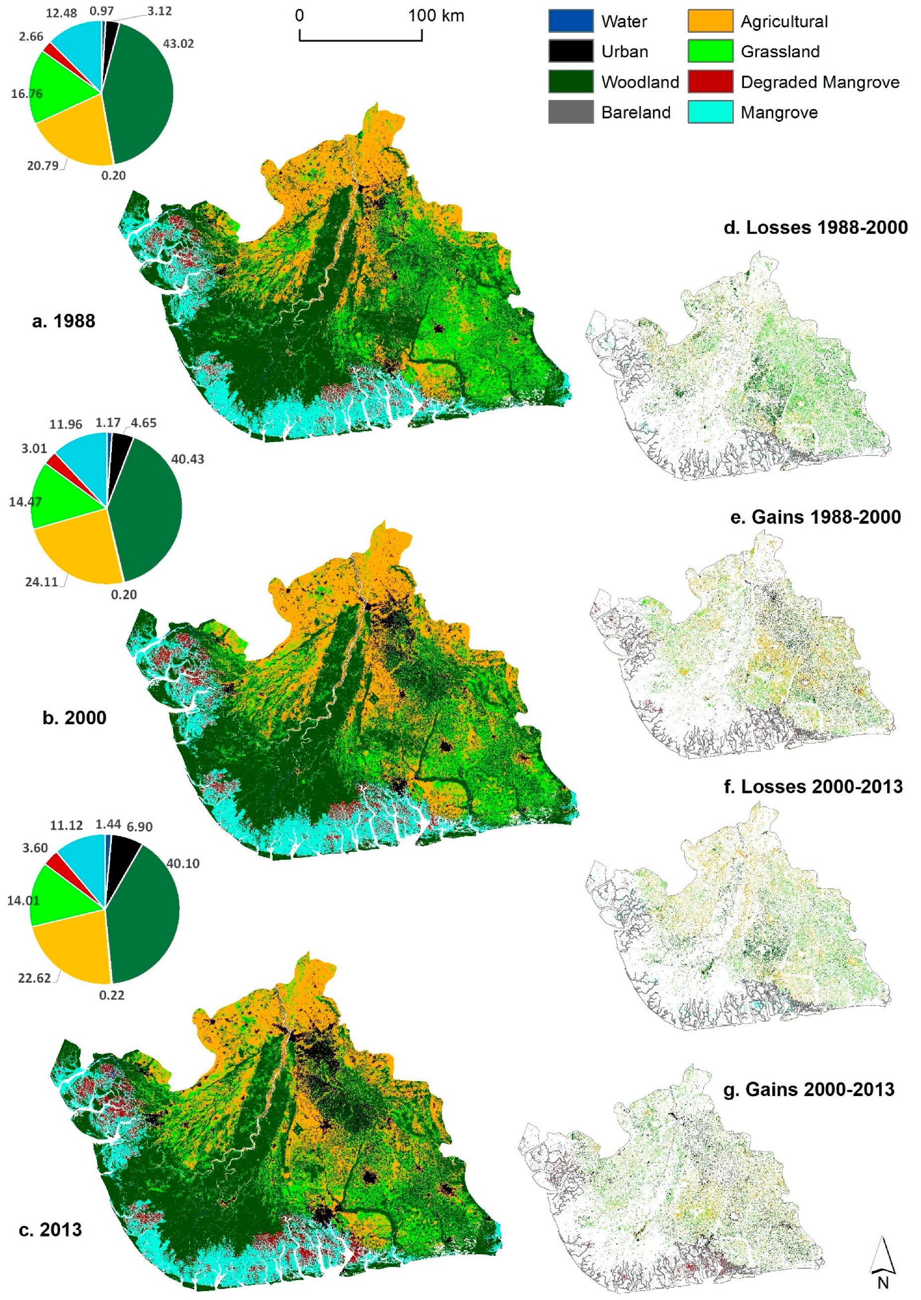
- There is consistent net loss in mangrove and woodland types and a consistent net gain of the urban class in both periods of study
- The area covered by non-degraded mangroves was reduced by ~250 km2 in each period (=Gross Loss – Gross Gain)
- About 10% of mangroves are degraded in each interval, and an additional 34 km2 of mangrove were converted to urban land use in both periods
- A portion of degraded mangrove is able to bounce back into its healthier state
- The net loss for the woodland class was more than 700 km2 in each period. A part of this class is converted to grasses (~8% and ~9%) and to agricultural land (~7% and ~5%)
- A quarter of the area mapped as grassland in the initial dates is converted to woodland by the end date
- The built-up areas increased by 47% (~900 km2) in the first period, an area larger than the size of New York City. In the second period, the increase was smaller (~800 km2) but still it amounted to 27% of the area covered in 2000
5.2. Fragmentation and Degradation of the Niger Delta Mangrove Forest
6. Conclusions
Supplementary Materials
Author Contributions
Funding
Acknowledgments
Conflicts of Interest
References
- Foufoula-Georgiou, E. A vision for a coordinated international effort on delta sustainability. Deltas Landf. Ecosyst. Hum. Act. 2013, 358, 3–11. [Google Scholar]
- Ericson, J.P.; Vorosmarty, C.J.; Dingman, S.L.; Ward, L.G.; Meybeck, M. Effective sea-level rise and deltas: Causes of change and human dimension implications. Glob. Planet. Chang. 2006, 50, 63–82. [Google Scholar] [CrossRef]
- Szabo, S.; Renaud, F.G.; Hossain, M.S.; Sebesvári, Z.; Matthews, Z.; Foufoula-Georgiou, E.; Nicholls, R.J. Sustainable development goals offer new opportunities for tropical delta regions. Environ. Sci. Policy Sustain. Dev. 2015, 57, 16–23. [Google Scholar] [CrossRef]
- Szabo, S.; Brondizio, E.; Renaud, F.G.; Hetrick, S.; Nicholls, R.J.; Matthews, Z.; Tessler, Z.; Tejedor, A.; Sebesvari, Z.; Foufoula-Georgiou, E. Population dynamics, delta vulnerability and environmental change: Comparison of the Mekong, Ganges–Brahmaputra and Amazon delta regions. Sustain. Sci. 2016, 11, 539–554. [Google Scholar] [CrossRef] [PubMed] [Green Version]
- Chow, J. Mangrove management for climate change adaptation and sustainable development in coastal zones. J. Sustain. For. 2018, 37, 139–156. [Google Scholar] [CrossRef]
- Goudie, A.S. The drainage of Africa since the cretaceous. Geomorphology 2005, 67, 437–456. [Google Scholar] [CrossRef]
- Spalding, M. World Atlas of Mangroves; Routledge: Abingdon-on-Thames, UK, 2010. [Google Scholar]
- Zabbey, N.; Hart, A.; Erondu, E. Functional roles of mangroves of the Niger Delta to the coastal communities and national economy. In Proceedings of the 25th Annual Conference of the Fisheries Society of Nigeria (FISON), Lagos, Nigeria, 25–29 October 2010. [Google Scholar]
- James, G.K.; Adegoke, J.O.; Saba, E.; Nwilo, P.; Akinyede, J. Satellite-based assessment of the extent and changes in the mangrove ecosystem of the Niger Delta. Mar. Geod. 2007, 30, 249–267. [Google Scholar] [CrossRef]
- Okonkwo, C.N.P.; Kumar, L.; Taylor, S. The Niger Delta wetland ecosystem: What threatens it and why should we protect it? Afr. J. Environ. Sci. Technol. 2015, 9, 451–463. [Google Scholar]
- Numbere, A. Impact of Hydrocarbon Pollution on the Mangrove Ecosystem of the Niger River Delta, Nigeria. Ph.D. Thesis, Saint Louis University, Saint Louis, MO, USA, 2014. [Google Scholar]
- NDDC. Niger Delta Regional Development Master Plan; Niger Delta Development Commission: Port Harcourt, Nigeria, 2006; pp. 48–99. [Google Scholar]
- World Bank. Defining an Environmental Development Strategy for the Niger Delta, Nigeria. Available online: http://documents.worldbank.org/curated/en/506921468098056629/pdf/multi-page.pdf (accessed on 18 October 2017).
- Kadafa, A.A. Oil Exploration and Spillage in the Niger Delta of Nigeria. Civil. Environ. Res. 2012, 2, 38–51. [Google Scholar]
- Balogun, T.F. Mapping impacts of crude oil theft and illegal refineries on mangrove of the Niger Delta of Nigeria with remote sensing technology. Mediterr. J. Soc. Sci. 2015, 6, 150. [Google Scholar] [CrossRef] [Green Version]
- Onyena, A.P.; Sam, K. A review of the threat of oil exploitation to mangrove ecosystem: Insights from Niger Delta, Nigeria. Glob. Ecol. Conserv. 2020, 22, e00961. [Google Scholar] [CrossRef]
- Duke, N.C. Oil spill impacts on mangroves: Recommendations for operational planning and action based on a global review. Mar. Pollut. Bull. 2016, 109, 700–715. [Google Scholar] [CrossRef] [PubMed]
- Twumasi, Y.A.; Merem, E.C. GIS and remote sensing applications in the assessment of change within a coastal environment in the Niger Delta region of Nigeria. Int. J. Environ. Res. Public Health 2006, 3, 98–106. [Google Scholar] [CrossRef]
- Nwobi, C.; Williams, M.; Mitchard, E.T.A. Rapid Mangrove Forest Loss and Nipa Palm (Nypa fruticans) Expansion in the Niger Delta, 2007–2017. Remote Sens. 2020, 12, 2344. [Google Scholar] [CrossRef]
- Uyigue, E.; Agho, M. Coping with Climate Change and Environmental Degradation in the Niger Delta of Southern Nigeria; Community Research and Development Centre Nigeria (CREDC): Benin City, Nigeria, 2007. [Google Scholar]
- Okali, D.; Eleri, E.O. Climate Change and Nigeria: A Guide for Policy Makers; Nigerian Environmental Study Action Team (NEST): Ibadan, Nigeria, 2004. [Google Scholar]
- Awosika, L.F. Impacts of Global Climate Change and Sea Level Rise on Coastal Resources and Energy Development in Nigeria. In Global Climate Change: Impact on Energy Development; Umolu, J.C., Ed.; DAMTECH Nigeria Limited: Jos, Nigeria, 1995. [Google Scholar]
- Ayanlade, A.; Drake, N. Forest loss in different ecological zones of the Niger Delta, Nigeria: Evidence from remote sensing. Geojournal 2016, 81, 717–735. [Google Scholar] [CrossRef]
- Mena, C.F. Trajectories of land-use and land-cover in the northern Ecuadorian Amazon: Temporal composition, spatial configuration, and probability of change. Photogramm. Eng. Remote Sens. 2008, 74, 737–751. [Google Scholar] [CrossRef]
- Gao, J.; Liu, Y.S. Determination of land degradation causes in Tongyu County, Northeast China via land cover change detection. Int. J. Appl. Earth Obs. Geoinf. 2010, 12, 9–16. [Google Scholar] [CrossRef]
- Obiefuna, J.N.; Nwilo, P.C.; Atagbaza, A.O.; Okolie, C.J. Land Cover Dynamics Associated with the Spatial Changes in the Wetlands of Lagos/Lekki Lagoon System of Lagos, Nigeria. J. Coast. Res. 2013, 29, 671–679. [Google Scholar] [CrossRef]
- Kuenzer, C.; van Beijma, S.; Gessner, U.; Dech, S. Land surface dynamics and environmental challenges of the Niger Delta, Africa: Remote sensing-based analyses spanning three decades (1986–2013). Appl. Geogr. 2014, 53, 354–368. [Google Scholar] [CrossRef]
- Kirui, K.B.; Kairo, J.G.; Bosire, J.; Viergever, K.M.; Rudra, S.; Huxham, M.; Briers, R.A. Mapping of mangrove forest land cover change along the Kenya coastline using Landsat imagery. Ocean Coast. Manag. 2013, 83, 19–24. [Google Scholar] [CrossRef]
- Martinuzzi, S.; Gould, W.A.; González, O.M.R. Creating Cloud-Free Landsat ETM+ Data Sets in Tropical Landscapes: Cloud and Cloud-Shadow Removal; Gen. Tech. Rep. IITF-32; U.S. Department of Agriculture, Forest Service, International Institute of Tropical Forestry: Washington, DC, USA, 2007. [Google Scholar]
- Colby, J.D.; Keating, P.L. Land cover classification using Landsat TM imagery in the tropical highlands: The influence of anisotropic reflectance (vol 19, pg 1479, 2001). Int. J. Remote Sens. 2001, 22, 2655–2656. [Google Scholar]
- Okoro, S.U.; Schickhoff, U.; Bohner, J.; Schneider, U.A. A novel approach in monitoring land-cover change in the tropics: Oil palm cultivation in the Niger Delta, Nigeria. Erde 2016, 147, 40–52. [Google Scholar] [CrossRef]
- Frantz, D. FORCE—Landsat+ Sentinel-2 analysis ready data and beyond. Remote Sens. 2019, 11, 1124. [Google Scholar] [CrossRef] [Green Version]
- Griffiths, P.; van der Linden, S.; Kuemmerle, T.; Hostert, P. Pixel-Based Landsat Compositing Algorithm for Large Area Land Cover Mapping. IEEE J. Sel. Top. Appl. Earth Obs. Remote Sens. 2013, 6, 2088–2101. [Google Scholar] [CrossRef]
- Mueller, H.; Rufin, P.; Griffiths, P.; Siqueira, A.J.B.; Hostert, P. Mining dense Landsat time series for separating cropland and pasture in a heterogeneous Brazilian savanna landscape. Remote Sens. Environ. 2015, 156, 490–499. [Google Scholar] [CrossRef] [Green Version]
- Hansen, M.C.; Egorov, A.; Roy, D.P.; Potapov, P.; Ju, J.; Turubanova, S.; Kommareddy, I.; Loveland, T.R. Continuous fields of land cover for the conterminous United States using Landsat data: First results from the Web-Enabled Landsat Data (WELD) project. Remote Sens. Lett. 2011, 2, 279–288. [Google Scholar] [CrossRef]
- Verhulp, J.; Denner, M. The Development of the South African National Land Cover Mapping Program: Progress and Challenges. Available online: http://www.africageoproceedings.org.za/wp-content/uploads/2014/08/119_Verhulp_Denner1.pdf (accessed on 26 October 2020).
- Basuki, T.M.; Skidmore, A.K.; Hussin, Y.A.; Van Duren, I. Estimating tropical forest biomass more accurately by integrating ALOS PALSAR and Landsat-7 ETM+ data. Int. J. Remote Sens. 2013, 34, 4871–4888. [Google Scholar] [CrossRef] [Green Version]
- Nascimento, W.R.; Souza, P.W.M.; Proisy, C.; Lucas, R.M.; Rosenqvist, A. Mapping changes in the largest continuous Amazonian mangrove belt using object-based classification of multisensor satellite imagery. Estuar. Coast. Shelf Sci. 2013, 117, 83–93. [Google Scholar] [CrossRef]
- Kamal, M.; Phinn, S.; Johansen, K. Object-Based Approach for Multi-Scale Mangrove Composition Mapping Using Multi-Resolution Image Datasets. Remote Sens. 2015, 7, 4753–4783. [Google Scholar] [CrossRef] [Green Version]
- Wicaksono, P. Mangrove above-ground carbon stock mapping of multi-resolution passive remote-sensing systems. Int. J. Remote Sens. 2017, 38, 1551–1578. [Google Scholar] [CrossRef]
- Bunting, P.; Rosenqvist, A.; Lucas, R.M.; Rebelo, L.M.; Hilarides, L.; Thomas, N.; Hardy, A.; Itoh, T.; Shimada, M.; Finlayson, C.M. The Global Mangrove WatchA New 2010 Global Baseline of Mangrove Extent. Remote Sens. 2018, 10, 1669. [Google Scholar] [CrossRef] [Green Version]
- Heumann, B.W. An object-based classification of mangroves using a hybrid decision tree—Support vector machine approach. Remote Sens. 2011, 3, 2440–2460. [Google Scholar] [CrossRef] [Green Version]
- Shirvani, Z.; Abdi, O.; Buchroithner, M.F. A new analysis approach for long-term variations of forest loss, fragmentation, and degradation resulting from road network expansion using Landsat time-series and object-based image analysis. Land Degrad. Dev. 2020, 31, 1462–1481. [Google Scholar] [CrossRef] [Green Version]
- Onojeghuo, A.O.; Blackburn, G.A. Forest transition in an ecologically important region: Patterns and causes for landscape dynamics in the Niger Delta. Ecol. Indic. 2011, 11, 1437–1446. [Google Scholar] [CrossRef]
- Salami, A.T.; Akinyede, J.; de Gier, A. A preliminary assessment of NigeriaSat-1 for sustainable mangrove forest monitoring. Int. J. Appl. Earth Obs. Geoinf. 2010, 12, S18–S22. [Google Scholar] [CrossRef]
- Kamwi, J.M.; Cho, M.A.; Kaetsch, C.; Manda, S.O.; Graz, F.P.; Chirwa, P.W. Assessing the Spatial Drivers of Land Use and Land Cover Change in the Protected and Communal Areas of the Zambezi Region, Namibia. Land 2018, 7, 131. [Google Scholar] [CrossRef] [Green Version]
- Geist, H.J.; Lambin, E.F. Proximate causes and underlying driving forces of tropical deforestation. Bioscience 2002, 52, 143–150. [Google Scholar] [CrossRef]
- Quezada, M.L.; Arroyo-Rodriguez, V.; Perez-Silva, E.; Aide, T.M. Land cover changes in the Lachua region, Guatemala: Patterns, proximate causes, and underlying driving forces over the last 50 years. Reg. Environ. Chang. 2014, 14, 1139–1149. [Google Scholar] [CrossRef]
- Campos, M.; Velazquez, A.; Verdinelli, G.B.; Skutsch, M.; Junca, M.B.; Priego-Santander, A.G. An interdisciplinary approach to depict landscape change drivers: A case study of the Ticuiz agrarian community in Michoacan, Mexico. Appl. Geogr. 2012, 32, 409–419. [Google Scholar] [CrossRef]
- Fernandez, G.F.C.; Obermeier, W.A.; Gerique, A.; Sandoval, M.F.L.; Lehnert, L.W.; Thies, B.; Bendix, J. Land Cover Change in the Andes of Southern Ecuador-Patterns and Drivers. Remote Sens. 2015, 7, 2509–2542. [Google Scholar] [CrossRef] [Green Version]
- Lei, C.G.; Wagner, P.D.; Fohrer, N. Identifying the most important spatially distributed variables for explaining land use patterns in a rural lowland catchment in Germany. J. Geogr. Sci. 2019, 29, 1788–1806. [Google Scholar] [CrossRef] [Green Version]
- Aldwaik, S.Z.; Pontius, R.G. Intensity analysis to unify measurements of size and stationarity of land changes by interval, category, and transition. Landsc. Urban Plan. 2012, 106, 103–114. [Google Scholar] [CrossRef]
- Gounaridis, D.; Zaimes, G.N.; Koukoulas, S. Quantifying spatio-temporal patterns of forest fragmentation in Hymettus Mountain, Greece. Comput. Environ. Urban Syst. 2014, 46, 35–44. [Google Scholar] [CrossRef]
- López, S.; López-Sandoval, M.F.; Gerique, A.; Salazar, J. Landscape change in Southern Ecuador: An indicator-based and multi-temporal evaluation of land use and land cover in a mixed-use protected area. Ecol. Indic. 2020, 115, 106357. [Google Scholar] [CrossRef]
- Coppin, P.; Jonckheere, I.; Nackaerts, K.; Muys, B.; Lambin, E. Digital change detection methods in ecosystem monitoring: A review. Int. J. Remote Sens. 2004, 25, 1565–1596. [Google Scholar] [CrossRef]
- Liu, H.; Zhou, Q. Developing urban growth predictions from spatial indicators based on multi-temporal images. Comput. Environ. Urban Syst. 2005, 29, 580–594. [Google Scholar] [CrossRef]
- Seto, K.C.; Fragkias, M. Mangrove conversion and aquaculture development in Vietnam: A remote sensing-based approach for evaluating the Ramsar Convention on Wetlands. Glob. Environ. Chang.-Hum. Policy Dimens. 2007, 17, 486–500. [Google Scholar] [CrossRef]
- Chen, X.W. Using remote sensing and GIS to analyse land cover change and its impacts on regional sustainable development. Int. J. Remote Sens. 2002, 23, 107–124. [Google Scholar] [CrossRef]
- NBS. National Population Projection; NBS: Abuja, Nigeria, 2018. [Google Scholar]
- World Resources Institute. IUCN—The World Conservation Union. In Global Biodiversity Strategy: Guidelines for Action to Save, Study, and Use Earth’s Biotic Wealth Sustainably and Equitably; World Resources Inst: Andrew Steer, DC, USA, 1992. [Google Scholar]
- Ugochukwu, C.N.; Ertel, J. Negative impacts of oil exploration on biodiversity management in the Niger De area of Nigeria. Impact Assess. Proj. Apprais. 2008, 26, 139–147. [Google Scholar]
- World Bank. GDP (Current US$)—Nigeria. Available online: https://data.worldbank.org/indicator/NY.GDP.MKTP.CD?end=2010&locations=NG&start=1960 (accessed on 2 August 2020).
- Ako, R.T. Nigeria’s Land Use Act: An anti-thesis to environmental justice. J. Afr. Law 2009, 53, 289–304. [Google Scholar] [CrossRef]
- Imevbore, V.; Imevbore, A.; Gundlach, E. Niger Delta Environmental Surveys: Vol-1-Environmental and Socio-Economic Characteristics; Environmental Resources Managers Ltd.: Lagos, Nigeria, 1997. [Google Scholar] [CrossRef]
- Safriel, U.; Adeel, Z. Development paths of drylands: Thresholds and sustainability. Sustain. Sci. 2008, 3, 117–123. [Google Scholar] [CrossRef]
- Thomas, N.; Lucas, R.; Bunting, P.; Hardy, A.; Rosenqvist, A.; Simard, M. Distribution and drivers of global mangrove forest change, 1996–2010. PLoS ONE 2017, 12, e0179302. [Google Scholar] [CrossRef] [Green Version]
- ESRI. ArcGIS Pro. Available online: https://www.esri.com/en-us/arcgis/products/arcgis-pro/overview (accessed on 25 September 2020).
- Maxar; Technologies. Imagery Basemaps. Available online: https://www.maxar.com/products/imagery-basemaps (accessed on 25 September 2020).
- Masek, J.G.; Vermote, E.F.; Saleous, N.E.; Wolfe, R.; Hall, F.G.; Huemmrich, K.F.; Gao, F.; Kutler, J.; Lim, T.K. A Landsat surface reflectance dataset for North America, 1990-2000. IEEE Geosci. Remote Sens. Lett. 2006, 3, 68–72. [Google Scholar] [CrossRef]
- Zhu, Z.; Woodcock, C.E. Object-based cloud and cloud shadow detection in Landsat imagery. Remote Sens. Environ. 2012, 118, 83–94. [Google Scholar] [CrossRef]
- Tucker, C.J. Red and photographic infrared linear combinations for monitoring vegetation. Remote Sens. Environ. 1979, 8, 127–150. [Google Scholar] [CrossRef] [Green Version]
- Symeonakis, E.; Higginbottom, T.P.; Petroulaki, K.; Rabe, A. Optimisation of Savannah Land Cover Characterisation with Optical and SAR Data. Remote Sens. 2018, 10, 499. [Google Scholar] [CrossRef] [Green Version]
- Higginbottom, T.P.; Symeonakis, E.; Meyer, H.; van der Linden, S. Mapping fractional woody cover in semi-arid savannahs using multi-seasonal composites from Landsat data. ISPRS J. Photogramm. Remote Sens. 2018, 139, 88–102. [Google Scholar] [CrossRef] [Green Version]
- Haralick, R.M. Statistical and structural approaches to texture. Proc. IEEE 1979, 67, 786–804. [Google Scholar] [CrossRef]
- Thapa, R.B.; Watanabe, M.; Motohka, T.; Shimada, M. Potential of high-resolution ALOS-PALSAR mosaic texture for aboveground forest carbon tracking in tropical region. Remote Sens. Environ. 2015, 160, 122–133. [Google Scholar] [CrossRef]
- Cohen, W.B.; Yang, Z.G.; Kennedy, R. Detecting trends in forest disturbance and recovery using yearly Landsat time series: 2. TimeSync—Tools for calibration and validation. Remote Sens. Environ. 2010, 114, 2911–2924. [Google Scholar] [CrossRef]
- Pal, M. Random forest classifier for remote sensing classification. Int. J. Remote Sens. 2005, 26, 217–222. [Google Scholar] [CrossRef]
- Team, R.C. R: A Language and Environment for Statistical Computing. R Foundation for Statistical Computing, Vienna. 2017. Available online: https://www.R-Project.org (accessed on 26 October 2020).
- Pontius, R.G.; Gao, Y.; Giner, N.M.; Kohyama, T.; Osaki, M.; Hirose, K. Design and interpretation of intensity analysis illustrated by land change in Central Kalimantan, Indonesia. Land 2013, 2, 351–369. [Google Scholar] [CrossRef]
- McGarigal, K. FRAGSTATS: Spatial Pattern Analysis Program for Quantifying Landscape Structure; US Department of Agriculture, Forest Service, Pacific Northwest Research Station: Corvallis, OR, USA, 1995; Volume 351. [Google Scholar]


| Name | Abbreviation | Description |
|---|---|---|
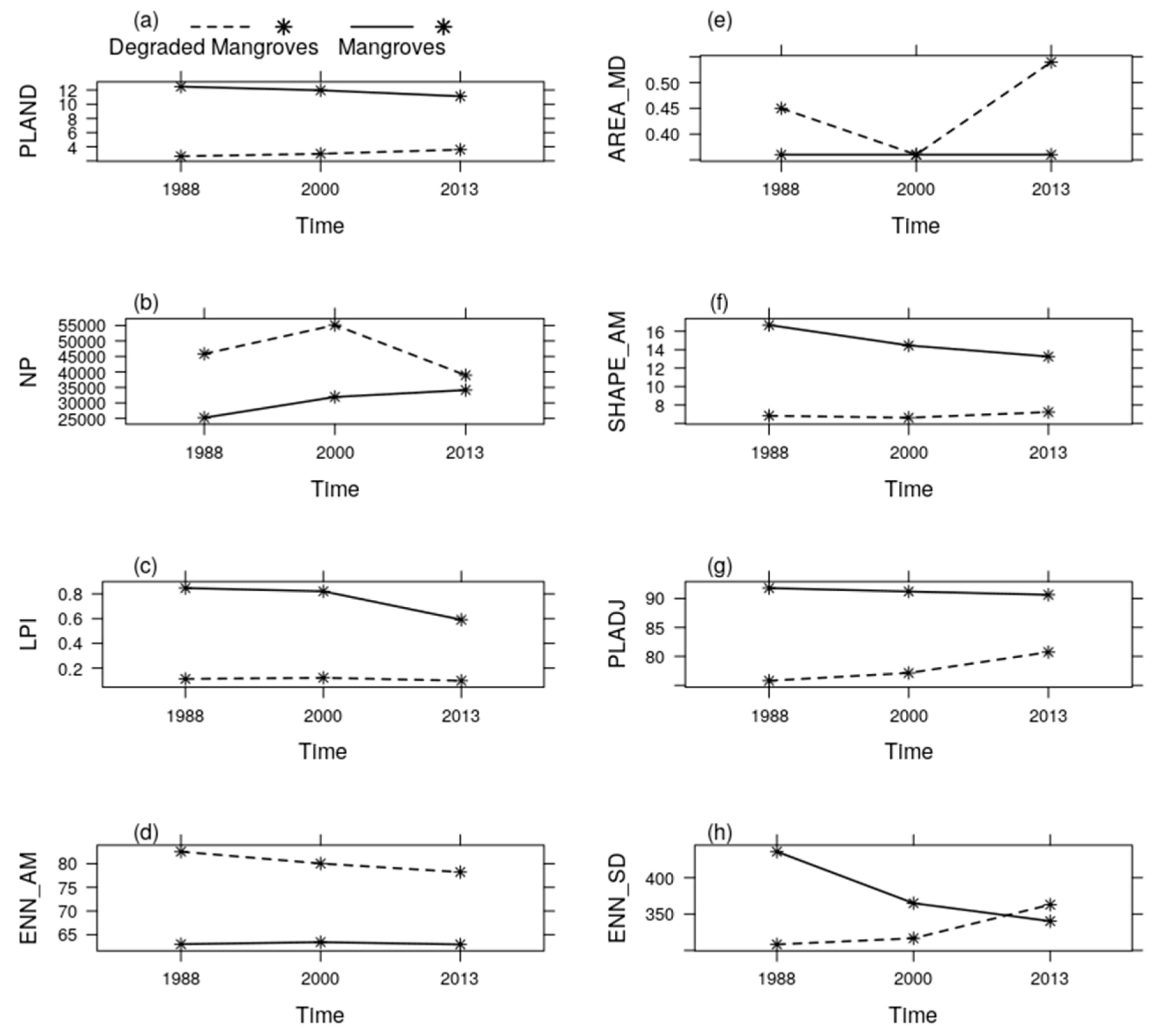
| Percentage of Landscape (%) | PLAND | Class percentage in landscape (proportional abundance) |
| Patch area median (ha) | AREA_MD | The median of patch areas in a class (a summary metric for the size of patches in the class, which is not influenced by very large patches) |
| Number of patches | NP | The number of patches in each class (simple measure of fragmentation) |
| Area weighted Mean Patch Shape Index | SHAPE_AM | Patch shape complexity at class level (indicative of changes at the edges) |
| Largest Patch Index (%) | LPI | Percentage of total landscape area occupied by the largest-sized patch (measure of dominance) |
| Percentage of like adjacencies (%) | PLADJ | The proportions of like adjacencies to the total number of adjacencies for the class’ cells (aggregation) |
| Area weighted mean Euclidean nearest neighbour distance (m) | ENN_AM | Euclidean distance measured form patch edge to the closest patch edge from the same class (measures patch dispersion). Here we use the area weighted mean for the class to balance the influence of large patches. |
| Euclidean nearest neighbour distance Standard Deviation | ENN_SD | Measure of variation of ENN in the class (in comparison with the mean shows the form of distribution of patches in the class) |
| 1988 Landsat | 2000 Landsat | 2000 Landsat + JERS-1 | 2013 Landsat | 2013 Landsat + PALSAR-2 | |||||||||||
|---|---|---|---|---|---|---|---|---|---|---|---|---|---|---|---|
| Overall Accuracy | 79.48 | 82.36 | 82.61 | 81.27 | 82.09 | ||||||||||
| 95% CI | ±0.003 | ±0.0029 | ±0.003 | ±0.0027 | ±0.0026 | ||||||||||
| C | PA | UA | C | PA | UA | C | PA | UA | C | PA | UA | C | PA | UA | |
| Wa | 73 | 79 | 73 | 75 | 85 | 75 | 75 | 83 | 75 | 74 | 85 | 74 | 78 | 87 | 78 |
| U | 70 | 92 | 70 | 81 | 92 | 81 | 81 | 96 | 81 | 84 | 92 | 84 | 88 | 92 | 88 |
| Wo | 84 | 79 | 84 | 87 | 83 | 87 | 87 | 83 | 87 | 84 | 85 | 84 | 84 | 85 | 84 |
| B | 61 | 77 | 61 | 49 | 84 | 49 | 48 | 80 | 48 | 50 | 85 | 50 | 50 | 86 | 50 |
| A | 81 | 80 | 81 | 88 | 81 | 88 | 88 | 81 | 90 | 88 | 79 | 88 | 87 | 79 | 87 |
| G | 71 | 65 | 71 | 53 | 65 | 53 | 54 | 64 | 54 | 56 | 65 | 56 | 57 | 64 | 57 |
| DM | 77 | 82 | 77 | 78 | 86 | 78 | 79 | 85 | 79 | 86 | 82 | 86 | 87 | 82 | 87 |
| M | 91 | 90 | 91 | 90 | 90 | 90 | 91 | 90 | 91 | 90 | 92 | 90 | 90 | 93 | 90 |
| a | 2000 (km2) | ||||||||||
| Wa | U | Wo | B | A | G | DM | M | 1988 total | Gross loss | ||
| 1988 | Wa | 395.70 | 9.34 | 3.59 | 12.93 | 7.72 | 0.63 | 51.66 | 20.58 | 502.16 | 106.46 |
| U | 4.30 | 1444.71 | 95.36 | 4.59 | 341.98 | 85.32 | 6.09 | 7.56 | 1989.91 | 545.20 | |
| Wo | 11.61 | 310.44 | 193,54.71 | 3.60 | 1655.90 | 2020.54 | 49.81 | 363.90 | 23,770.52 | 4415.81 | |
| B | 10.10 | 10.09 | 0.30 | 72.67 | 19.14 | 0.19 | 0.12 | 0.28 | 112.90 | 40.23 | |
| A | 20.52 | 543.09 | 647.15 | 39.38 | 8868.25 | 1439.74 | 7.48 | 5.89 | 11,571.48 | 2703.24 | |
| G | 0.55 | 572.51 | 2419.61 | 0.87 | 2883.36 | 3534.56 | 1.62 | 8.34 | 9421.41 | 5886.86 | |
| DM | 149.47 | 8.17 | 13.41 | 0.35 | 3.45 | 1.64 | 1169.07 | 454.69 | 1800.27 | 631.20 | |
| M | 40.90 | 26.06 | 536.28 | 0.64 | 8.09 | 6.00 | 535.47 | 5743.70 | 6897.15 | 1153.45 | |
| 2000 Total | 633.15 | 2924.41 | 230,70.43 | 135.03 | 13,787.88 | 7088.63 | 1821.33 | 6604.94 | |||
| Gross Gain | 237.46 | 1479.70 | 3715.71 | 62.36 | 4919.64 | 3554.07 | 652.25 | 861.24 | |||
| b | 2013 (km2) | 2000 Total | Gross Loss | ||||||||
| 2000 | Wa | 522.59 | 2.09 | 4.91 | 10.26 | 4.16 | 0.48 | 76.77 | 13.16 | 634.42 | 111.83 |
| U | 19.64 | 2150.29 | 173.38 | 18.35 | 357.87 | 184.36 | 10.72 | 10.19 | 2924.80 | 774.51 | |
| Wo | 10.12 | 371.43 | 18,959.22 | 21.03 | 1251.56 | 2038.85 | 67.20 | 351.52 | 230,70.92 | 4111.70 | |
| B | 58.00 | 5.09 | 1.99 | 57.13 | 12.33 | 0.38 | 0.09 | 0.09 | 135.10 | 77.97 | |
| A | 25.86 | 933.43 | 939.59 | 46.28 | 9083.42 | 2754.41 | 3.55 | 1.58 | 13,788.12 | 4704.71 | |
| G | 1.34 | 253.81 | 1784.19 | 5.44 | 1922.06 | 3113.85 | 5.57 | 2.38 | 7088.64 | 3974.79 | |
| DM | 157.76 | 3.64 | 26.83 | 5.21 | 4.52 | 2.07 | 1158.61 | 462.79 | 1821.42 | 662.81 | |
| M | 65.30 | 7.86 | 377.77 | 14.21 | 7.68 | 7.84 | 595.84 | 5529.72 | 6606.22 | 1076.50 | |
| 2013 Total | 860.61 | 3727.63 | 22267.88 | 177.91 | 12,643.6 | 8102.24 | 1918.34 | 6371.43 | |||
| Gross Gain | 338.02 | 1577.34 | 3308.66 | 120.78 | 3560.18 | 4988.39 | 759.74 | 841.71 | |||
| Transitions FROM | Mangrove | |||
|---|---|---|---|---|
| Time Interval | 1988–2000 | 2000–2013 | ||
| TO Category | Observed Annual Transition (km2) | Transition Intensity % of 2000 Category | Observed Annual Transition (km2) | Transition Intensity % of 2013 Category |
| Water | 206 | 0.03 | 332 | 0.05 |
| Urban | 717 | 0.03 | 540 | 0.02 |
| Woodland | 506 | 0.00 | 1431 | 0.01 |
| Bareland | 40 | 0.04 | 221 | 0.20 |
| Agricultural | 485 | 0.00 | 298 | 0.00 |
| Grassland | 244 | 0.00 | 461 | 0.01 |
| Deg. Mangrove | 23,799 | 1.57 | 32,742 | 1.80 |
Publisher’s Note: MDPI stays neutral with regard to jurisdictional claims in published maps and institutional affiliations. |
© 2020 by the authors. Licensee MDPI, Basel, Switzerland. This article is an open access article distributed under the terms and conditions of the Creative Commons Attribution (CC BY) license (http://creativecommons.org/licenses/by/4.0/).
Share and Cite
Nababa, I.I.; Symeonakis, E.; Koukoulas, S.; Higginbottom, T.P.; Cavan, G.; Marsden, S. Land Cover Dynamics and Mangrove Degradation in the Niger Delta Region. Remote Sens. 2020, 12, 3619. https://0-doi-org.brum.beds.ac.uk/10.3390/rs12213619
Nababa II, Symeonakis E, Koukoulas S, Higginbottom TP, Cavan G, Marsden S. Land Cover Dynamics and Mangrove Degradation in the Niger Delta Region. Remote Sensing. 2020; 12(21):3619. https://0-doi-org.brum.beds.ac.uk/10.3390/rs12213619
Chicago/Turabian StyleNababa, Iliya Ishaku, Elias Symeonakis, Sotirios Koukoulas, Thomas P. Higginbottom, Gina Cavan, and Stuart Marsden. 2020. "Land Cover Dynamics and Mangrove Degradation in the Niger Delta Region" Remote Sensing 12, no. 21: 3619. https://0-doi-org.brum.beds.ac.uk/10.3390/rs12213619