Article

Implementation of Artificial Intelligence Based Ensemble Models for Gully Erosion Susceptibility Assessment

by
Indrajit Chowdhuri
1,
Subodh Chandra Pal
1,
Alireza Arabameri
2,
Asish Saha
1,
Rabin Chakrabortty
1,
Thomas Blaschke
3,
Biswajeet Pradhan
4,5,6,7 and
Shahab. S. Band
8,*
1
Department of Geography, The University of Burdwan, Bardhaman, West Bengal 713104, India
2
Department of Geomorphology, Tarbiat Modares University, Tehran 14117-13116, Iran
3
Department of Geoinformatics–Z_GIS, University of Salzburg, 5020 Salzburg, Austria
4
Centre for Advanced Modelling and Geospatial Information Systems (CAMGIS), Faculty of Engineering and Information Technology, University of Technology Sydney, Ultimo NSW 2007, Australia
5
Department of Energy and Mineral Resources Engineering, Sejong University, Choongmu-gwan, 209 Neungdong-ro, Gwangjin-gu, Seoul 05006, Korea
6
Center of Excellence for Climate Change Research, King Abdulaziz University, P.O. Box 80234, Jeddah 21589, Saudi Arabia
7
Earth Observation Center, Institute of Climate Change, Universiti Kebangsaan Malaysia, Bangi 43600 UKM, Selangor, Malaysia
8
Future Technology Research Center, College of Future, National Yunlin University of Science and 21 Technology, 123 University Road, Section 3, Douliou, Yunlin 64002, Taiwan
*
Author to whom correspondence should be addressed.
Remote Sens. 2020, 12(21), 3620; https://0-doi-org.brum.beds.ac.uk/10.3390/rs12213620
Submission received: 5 October 2020 / Revised: 1 November 2020 / Accepted: 2 November 2020 / Published: 4 November 2020

Abstract

:
The Rarh Bengal region in West Bengal, particularly the eastern fringe area of the Chotanagpur plateau, is highly prone to water-induced gully erosion. In this study, we analyzed the spatial patterns of a potential gully erosion in the Gandheswari watershed. This area is highly affected by monsoon rainfall and ongoing land-use changes. This combination causes intensive gully erosion and land degradation. Therefore, we developed gully erosion susceptibility maps (GESMs) using the machine learning (ML) algorithms boosted regression tree (BRT), Bayesian additive regression tree (BART), support vector regression (SVR), and the ensemble of the SVR-Bee algorithm. The gully erosion inventory maps are based on a total of 178 gully head-cutting points, taken as the dependent factor, and gully erosion conditioning factors, which serve as the independent factors. We validated the ML model results using the area under the curve (AUC), accuracy (ACC), true skill statistic (TSS), and Kappa coefficient index. The AUC result of the BRT, BART, SVR, and SVR-Bee models are 0.895, 0.902, 0.927, and 0.960, respectively, which show very good GESM accuracies. The ensemble model provides more accurate prediction results than any single ML model used in this study.

1. Introduction

The origin and development of gullies are related to water-induced soil erosion and are treated as a major global problem. The formation of gullies and their gradual expansion significantly alter the shape of the earth’s surface [1]. Therefore, gully formation that gradually changes the shape of the earth’s surface is often associated with the formation of badland geomorphic features, which is particularly impeding in production activities, the construction of road networks, and associated activities [2]. As a result, land degradation in the form of gully erosion is the major cause of loss of productive soil surface, affecting nearly 1 billion hectares globally [3,4]. Therefore, this type of hazardous phenomenon causes environmental degradation, threatening to the lives of others, as well as loss of economic activity. Therefore, to understand the formation and development of gullies and associated erosional activities, and to overcome this global problem in a sustainable way it is necessary to perform gully erosion susceptibility (GES) mapping. In general, gully formation is a complex phenomenon that depends mainly on extreme precipitation events and improper land use utilization, as well as lack of proper planning [5]. Basically, a gully can be defined as a permanent water channel with a temporary flow of water during phases of heavy rainfall, in which the sediment is carried down the slope. The formation of gully erosion is a combination of different sub-processes, and these are the retreat of sloping land through head-cut, piping, fluting, crack development by tensional activity, and mass wasting [6]. In general, gullies are classified into three categories based on depth, namely grooves (<0.3 m), shallow gullies (0.3 to 2 m), and deep gullies (>3 m) [5]. The origin and development of gullies are widely responsible for the extensive hot and dry periods followed by heavy rainfall, together with human land-use practices, particularly in the monsoon dominated hot-dry climatic area. There are two groups of factors for the occurrence of gullies, which are physical factors (topography, climate, soil texture, vegetation cover, etc.) and anthropogenic factors (over grazing, deforestation, land utilization in an unplanned way, etc.) [7]. It is also a very well-known fact that similar factors are not responsible for the occurrence of gullies throughout the several regions in this world. Therefore, depending on the unique topographical, climatological, and hydrological characteristics, the pattern of gullies occurrence, their morphology, and erosional activities vary from place to place.
As stated in the aforementioned paragraphs, soil erosion causes a huge amount of economic losses and is treated as a global threat. The economic losses caused by soil erosion in South Asia are nearly USD 5400 million caused by a loss of soil productivity affecting 36 million tons annually [8]. The phenomenon of land degradation caused by soil erosion in the form of gully erosion is a critical hazard that has already affected approximately 3.975 million hectares (Mha) of land across India [9]. According to the various reports, such as the Ministry of Agriculture (MoA) (in 1994) and the National Bureau of Soil Survey and Land Use Planning (NBSS and LUP) (in 2004), the land degradation rate in India is estimated to be 107.4 and 146.8 Mha, respectively [10,11]. According to the Government of India’s Ministry of Environment and Forestry’s (2011) report, water erosion is responsible for about 10.21% of the land degradation in India. The unique climatic characteristics in India, i.e., heavy rainfall during the monsoon season and temperature fluctuations throughout the year, are responsible for the formation of gullies and increase the erosional potential and sedimentation. Our study area in the Gandheswari river basin is enormously affected by land degradation through gully erosion as it is located in the extended part of the Chotanagpur plateau with a sub-tropical Indian climatic condition. In addition to these two aspects, agricultural activities, destruction of the soil structure through fertilizers, increasing deforestation, and a lack of proper drainage systems are also responsible for the formation and development of rill-gullies in this area. Therefore, it is necessary to prevent and mitigate the gully formation processes by ascertaining their spatial extent and evaluating their controlling factors. GES mapping is an appropriate tool to carry out this task in a sustainable and perspective way.
In general, qualitative and quantitative methods have been applied to analyze gully erosion and to perform GESM [12]. Basically, a qualitative analysis requires a geomorphological and heuristic approach and skilled persons’ knowledge, while quantitative methods are based on a perfect relationship among the gully erosion conditioning factors (GECFs) and numerical values representing the occurrence of gullies [13]. Over time, GESM has been carried out using various techniques and models. Initially, it was done using remote sensing, geographic information system (GIS), and statistical models [14]. Different types of statistical models including the frequency ratio, analytical hierarchical process (AHP) [15], certainty factor (CF) [16], weight of evidence (WoE) [17], and evidential belief function (EBF) [18] have been applied to assess GESM approaches. Then, machine learning (ML) algorithms have been used for their ability to handle a big dataset and discover the complex relationships among the various conditioning factors used in GESM. The most widely applied ML algorithms in GESM are the artificial neural network (ANN) [19], support vector machine (SVM) [19], random forest (RF) [20], boosted regression trees (BRT) [21], alternating decision tree (ADTree) [22], and the multi-layer perception approach (MLPC) [23]. More recently, ensemble techniques, i.e., an amalgamation of two or more statistical or ML models, have been used for GESM. Basically, ensemble models have been used to remove the shortcomings of individual statistical or ML models [24]. Therefore, keeping in view the fact of widely acceptance of ML algorithms among several research groups of people, due to their high accuracy assessment in the prediction result, in this study we also used three popular ML algorithms namely boosted regression tree (BRT), Bayesian additive regression tree (BART), support vector regression (SVR), and the ensemble of the SVR-Bee models, and as we know, the ensemble has a greater accuracy assessment than any single stand-alone ML model. It is also stated that in several literature studies as well as to the best of our knowledge, there is no such research work which is based on the ensemble of SVR-Bee model and BART algorithm on GESM. Therefore, the ensemble of SVR-Bee algorithm and their comparison with the three aforementioned ML models is the novelty of this research work for optimal prediction analysis of GESM. The literature study shows that various ML algorithms as well as statistical approacheshave been widely used in GESM by Ghosh and Guchhait [8,25], Hembrem et al. [26], Roy et al. [23], and Chakrabortty et al. [27,28] in the surrounding of the present research area, i.e., the extended part of Chotanagpur plateau region of Rarh Bengal in the eastern part of India. However, until now, no research work has been carried out in the present study area through the aforementioned ML methods used in the current research work. Therefore, we have also compared the prediction result produced by the current research work and another established research work’s result, which is based on other ML models, except the ML models used in this research study area for understanding the suitable and better accuracy performances of ML algorithms. In this research, we assessed the GESM of a sub-tropical watershed of the Gandheswaririver in West Bengal, India.
The main aim in this research study is to assess gully erosion susceptibility mapping. As we know, the foremost step for sustainable management of land degradation through gully-induced soil erosion is to prepare GESM in an accurate way. It is indeed necessary to map future gully erosion prone areas in order to minimize the adverse effect of gully-induced soil erosion and for the proper management of agricultural land, road networks, etc. Thus, to do so in this study, we have prepared gully erosion susceptibility maps through theensemble approach of SVR-Bee model and three other ML algorithms. Therefore, for progress in our research work, here we have chosen twenty favorable conditioning factors for the occurrence of gullies in this region. Alongside, several statistical indices were used for experimental analysis of the input data, i.e., several gully erosion conditioning factors (GECFs), and the validation and accuracy assessment of the prediction result produced by ML models. Finally, it is concluded that the main strategy in this research work is to map gully erosion susceptibility in an optimal way through applying three stand-alone ML algorithms and the ensemble approach. The final output result of gully erosion susceptibility maps can help planners and land management authorities make the best use of land resources for sustainable development within this particular basin area.

2. Materials and Methods

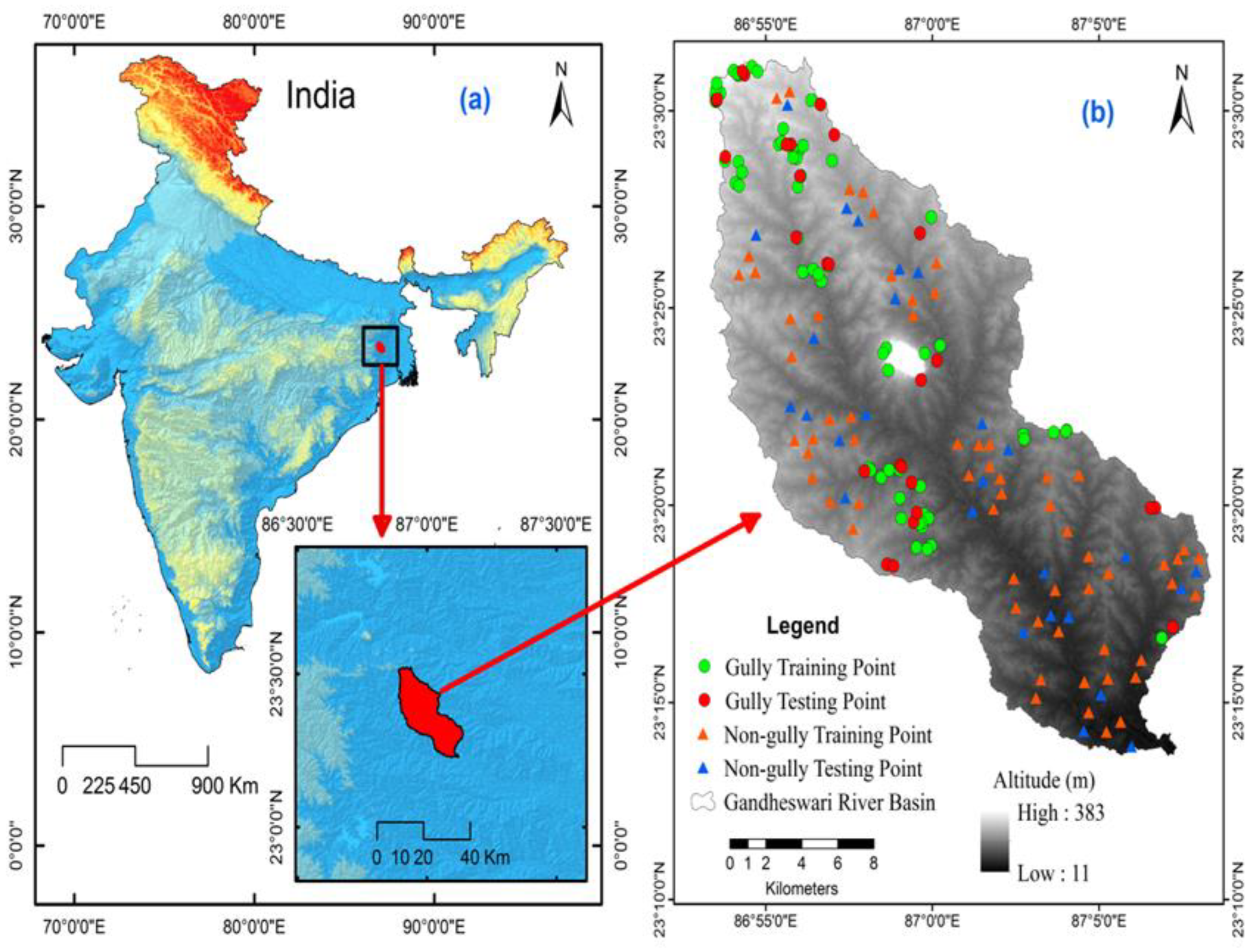
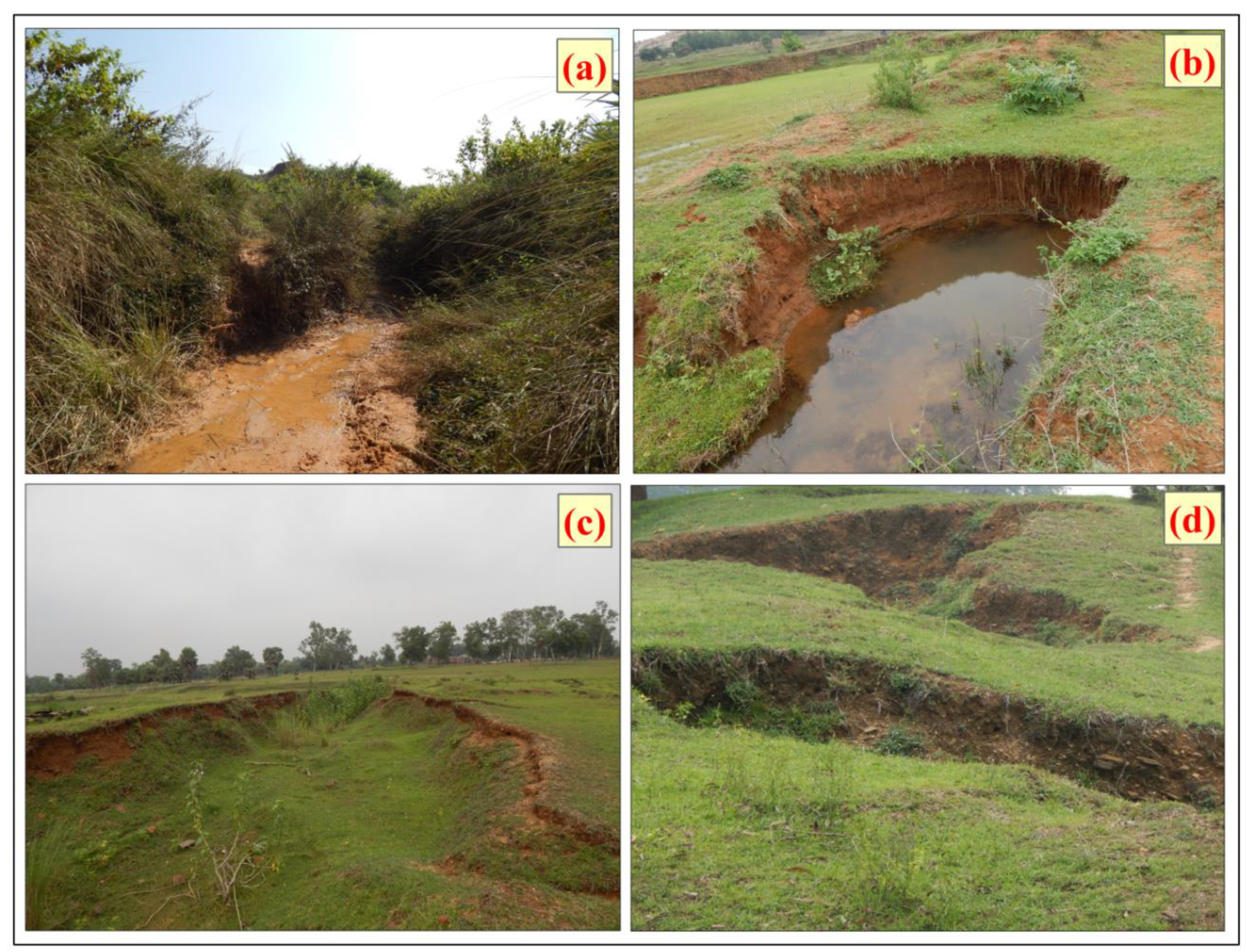
2.1. Description of the Study Area
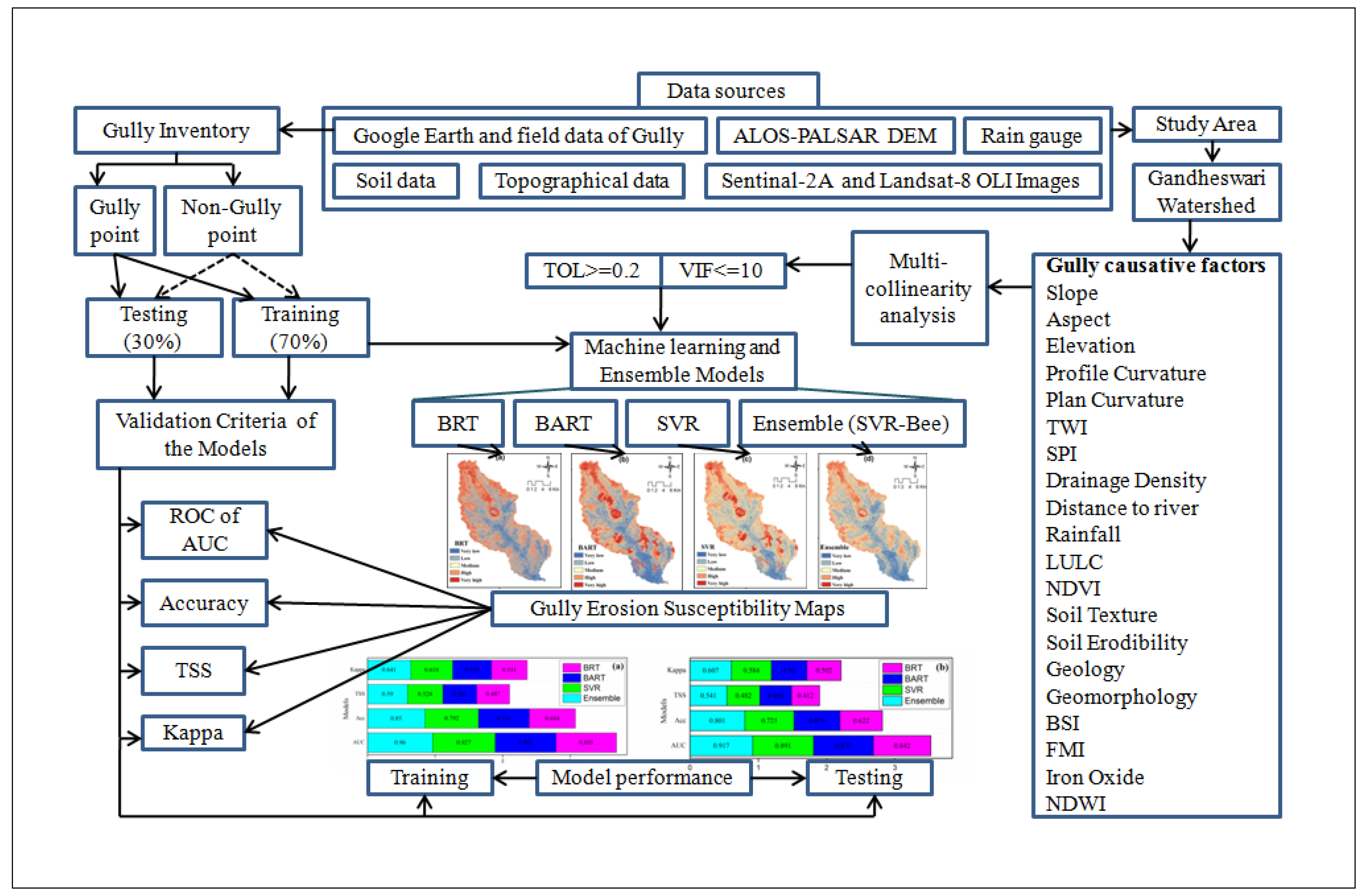
The Gandheswari river is a left-sided tributary in the upper course of the Dwarakeshwar river. This river originates near the Santuri Community Development Block (C.D. Block) of Purulia district of West Bengal [29]. The confluence point of the two rivers Dwarakeshwar and Gandheswari is at Bhutshahor, Bankura district of West Bengal, India. The total length of this river is 50.3 km from source to mouth and it covers an area of 392.69 sq. km. between latitudes 23°13′17″ and 23°31′27″ N and longitudes 86°53′12″ and 87°08′03″ E (Figure 1). The general direction of the slope in this basin area is towards the south-east [30]. The topography is undulating with the presence of several tiny rivulets [23]. Geologically, this study area is in the extended part of the Chotanagpur plateau along with the Rarh plains of Bengal [31]. Lateritic with mottled clay along with red, brown, and colluvial soils are found in the entire basin area. The climate is a sub-tropical monsoon with an average annual rainfall of about 1030 mm, whereby this mostly occurs in the monsoon season. The highest summer and lowest winter temperatures are about 42 and 10°C, respectively. The vegetation in this area is thin, with the most common plant species being several kinds of cacti and bushes along with Palas and Kusum hardwood trees.
In addition, the river basin is a unique region in terms of different physical characteristics such as the undulating plain of Chotanagpur plateau fringe, unconsolidated rock structure of Rajmahal formation, and the lateritic rocks and soil structure. In the hot-dry and seasonal moist climatic region, red lateritic soil has formed with a concentration of iron-aluminum oxides and the composition is very hard in nature. However, when the exposed hard lateritic comes in contact with rain water during the wet season, rocks are eroded by the head cut erosion. The overall parallel drainage systems over the plateau fringe dissect the lateritic Rarh Bengal into several patches. Some patches have been found as a bad land with extensive rill gully and ravine erosion. Due to the monsoonal rainfall, this region is facing several water-induced gully erosions, which has been reported in the literature [23,25,32,33]. In the present study area of Gandheswari river basin, a mainly elongated round head and steep wall with V shaped gully types have been found. Therefore, the land degradation problem has been noticed in this river basin, which affects agriculture, forestry, deformation of the land surface, etc. The major land use types in this region are single and double agricultural land, agro-forestry, very few patches of deciduous broadleaf forest, Shurbland, bare soil surface, and built-up land. In this area, no such protection measurement has been taken yet for controlling gully erosion, only the plantation of social-forestry has been adopted to control the same. Keeping in view the above fact, it has been observed that the rate of gully-induced soil erosion is very high in this area.

2.2. Methodology

The objective of this research work was completed in the following five steps (Figure 2).
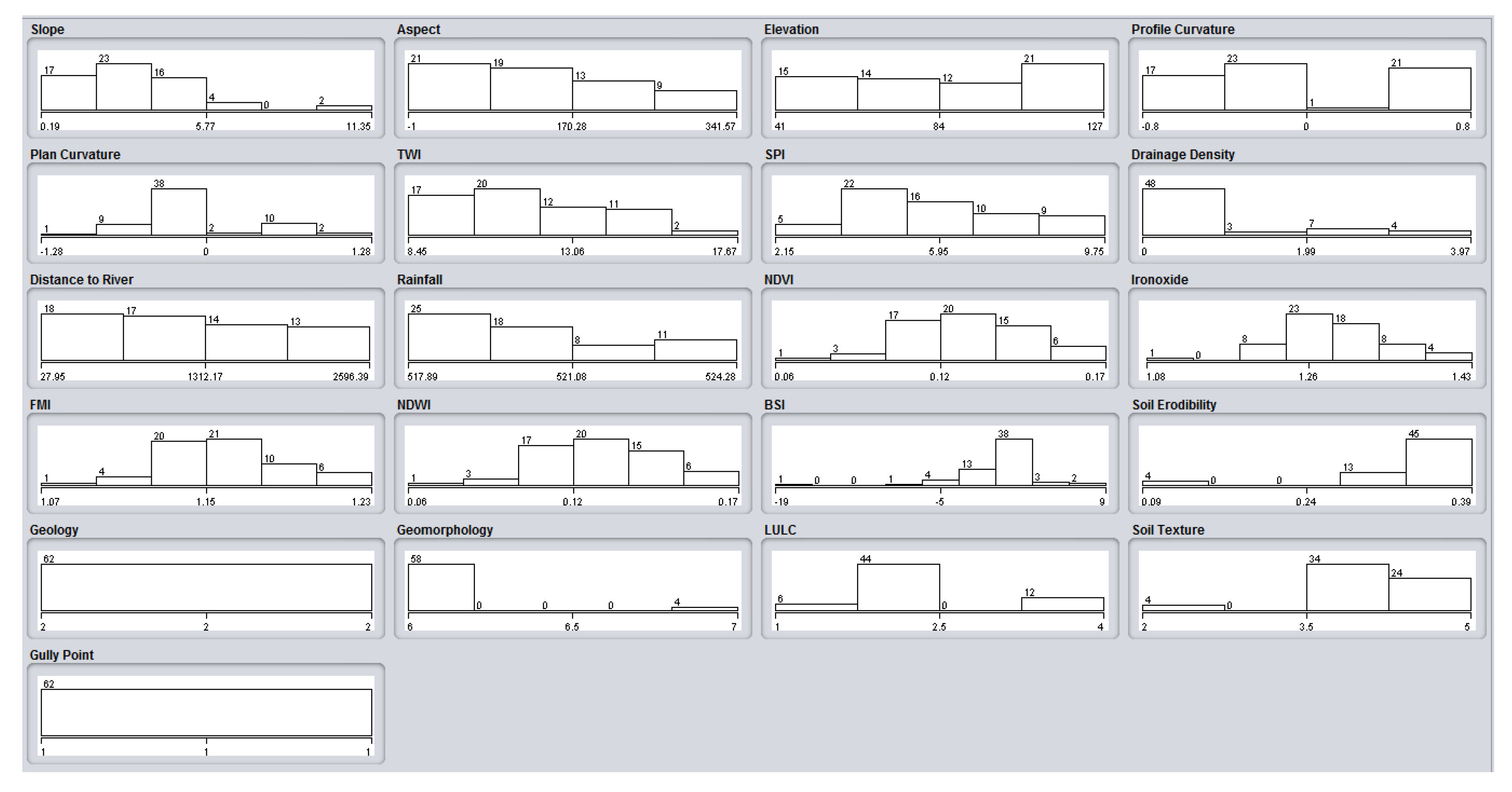
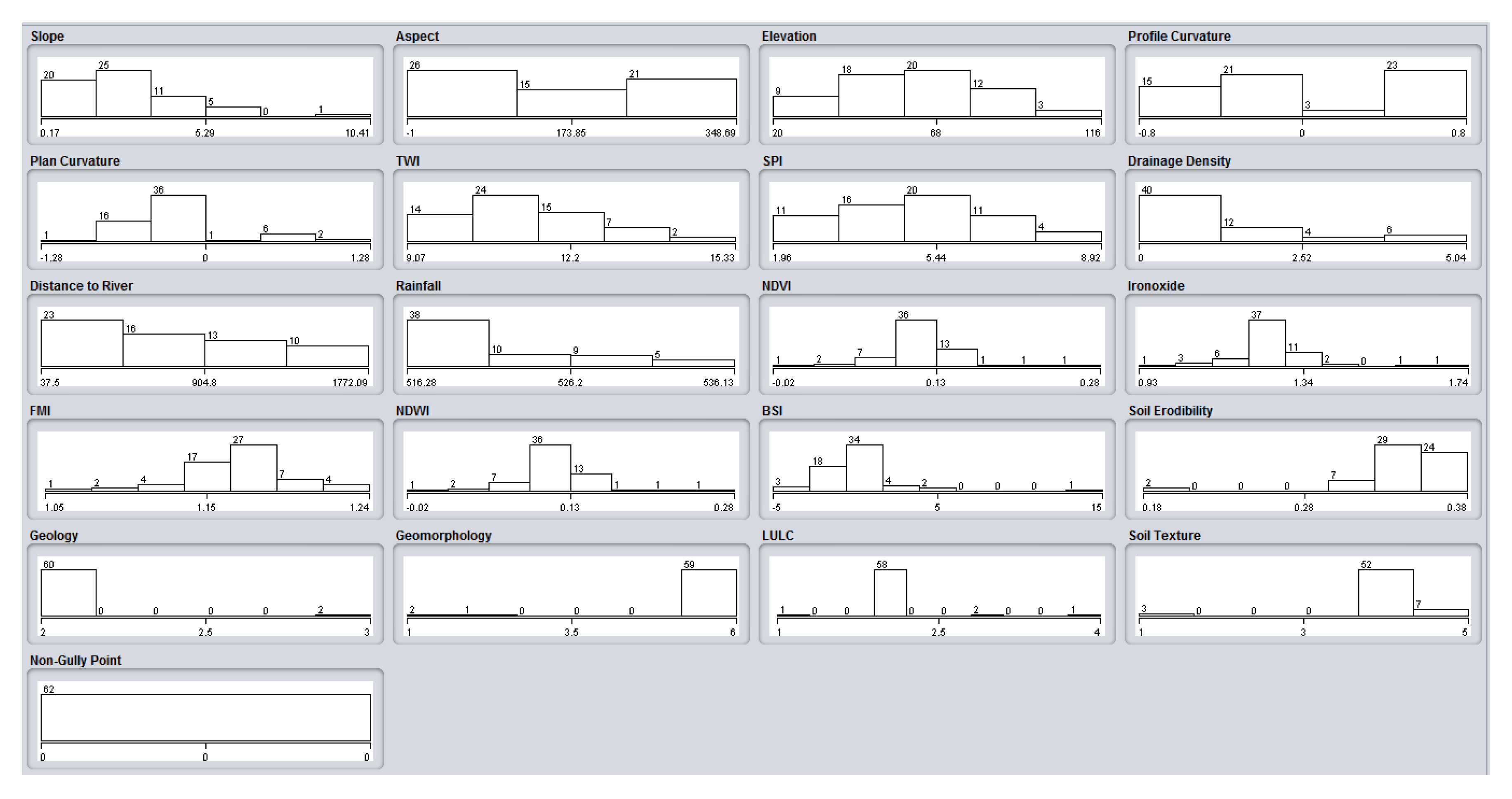
  • A total of 178 (89 each for gully and non-gully) gully erosion points were used to prepare a gully erosion inventory map. A total of 20 GECFs were used for the different GESMs.
  • The variance inflation factor (VIF) and tolerance (TOL) techniques were used for multi-collinearity (MC) analysis.
  • The importance of several GECFs was determined using the random forest (RF) algorithm and step-wise weight assessment ratio analysis (SWARA).
  • GESMs wereprepared based on the boosted regression tree (BRT), Bayesian additive regression tree (BART), support vector regression (SVR), ML models and the SVR-Bee ensemble model. All of these ML models and the ensemble approach were run in MATLAB and the ‘R’ statistical programming package by using the respective algorithms.
  • Every model was validated using the receiver operating characteristic curve with the area under curve (ROC-AUC), accuracy (ACC), true skill statistic (TSS), and the Kappa coefficient index analysis.
The methodology used in this study is described in detail as follows:
First, 178 randomly selected gully erosion points along with 20 GECFs were used to produce different gully erosion susceptibility maps. When researchers apply any linear statistical-based model, the multi-collinearity of the variables may decimate the accuracy of the model’s result [34]. Before applying the gully erosion susceptibility models, we checked the potential linear dependencies among the variables to avoid multi-collinearity among variables. When the TOL value is above 0.2, and the VIF value is below 10, there is no multi-collinearity among the variables. The GES maps in this study area were prepared using the ML algorithms of boosted regression tree (BRT), Bayesian additive regression tree (BART), support vector regression (SVR), and the ensemble of the SVR-Bee model. Due to some specific advantages, we used the abovementioned four models to analyze the GESMs. The advantage of the BRT model is that it is a non-parametric method used for measuring the relationships among the dependent and independent variables to forecast the analysis [35]. BART is a tree ensemble method that explains the variance of output product variables in a given dataset [20]. SVR is a supervised ML algorithm that is widely used in a complex dataset because it measures several curved boundaries. Any single ML model will have pros and cons in terms of susceptibility mapping and an ensemble method may potentially overcome some limitations. Therefore, we developed an ensemble SVR model with Bee algorithm methods for this study. The Bee algorithm generally helps solve the big data problems through modification and by calculating the fitness of the model [36]. The validation of the gully erosion susceptibility maps (GESMs) is an important step in the assessment of gully erosion susceptibility models. Previous researchers have used the receiver operating characteristic (ROC) curve with the area under the curve (AUC), accuracy (Acc), true skill statistic (TSS), and the Kappa index for the quantitative validation of GESMs prepared based on the BART, BRT, SVR, and the ensemble model [37,38,39]. The ROC curve is the most common technique used to quantitatively assess the model performance and the AUC of ROC has been used to measure the diagnostic ability of the model. Finally, all the models were validated using an ACC, ROC-AUC, TSS, and the Kappa coefficient index analysis.

2.2.1. Gully Erosion Inventory Map (GEIM)

Geomorphologists have used hypothesis criteria using different statistical analyses and predicting several natural hazard phenomena. In addition, this prediction is determined based on the past events, and an associated future prediction will be estimated through a functional relationship in the given datasets for various conditioning factors [18]. In GESM, it is very important to collect data that represent the dependent variables to make predictions using any model. In this study, we identified gully head-cut erosion points from Google Earth satellite imagery and intensive field surveys conducted with GPS to prepare an accurate GEIM. In general, the GEIM is used to evaluate the relationship between the distribution of gully head-cuts and several conditioning factors. Basically, the formation of gully head-cuts depends on topographical, lithological, climatic, and various other factors. Consequently, predicting the occurrence of gully head-cuts is largely dependent on the abovementioned factors. We identified a total of 89 gully head-cuts and included them in our GEIM. Of the total number of identified gully head-cuts, 70% (62 gully head-cut points) were selected for training the dataset, and the remaining 30% (27 gully head-cut points) were used to test the dataset. Similarly, 89 non-gully points were selected and divided to be used in training and testing the dataset (Figure 1). Some field photographs of gully head-cut points are shown in Figure 3.

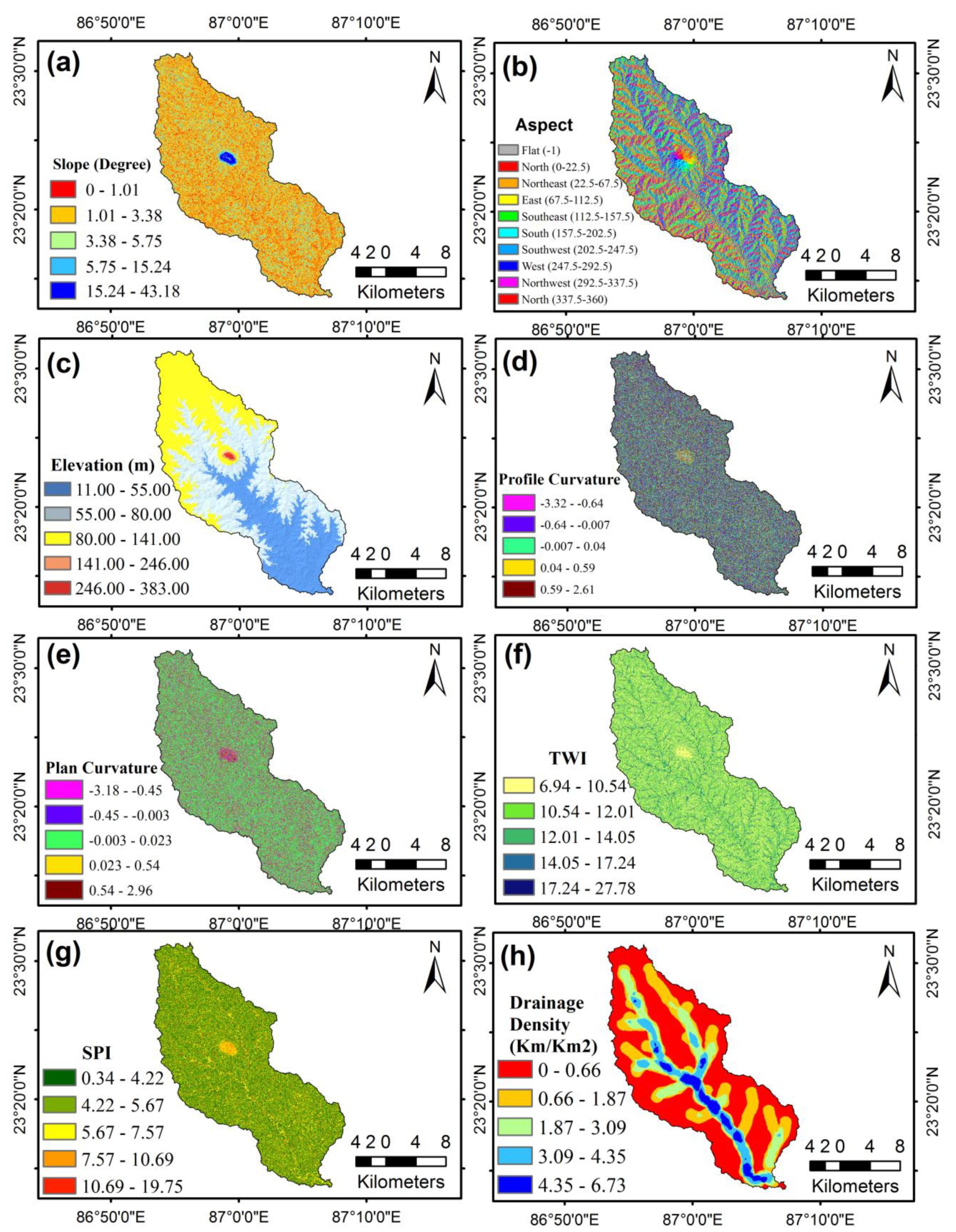
2.2.2. Gully Erosion Conditioning Factors (GECFs)

The first step in predicting the GESM is to select several suitable GECFs. Basically, GECFs have been divided into conditioning and triggering factors including environmental, topographical, geological, hydrological, climatological factors, etc. Despite this, there is no universal regulation for selecting the most appropriate GECFs. Therefore, we based our selection of GECFs on the geographical condition, variations in gully head-cut occurrences, and the models used in our analysis. To fulfill the objective of this research, we selected a total of 20 conditioning factors for GESM. These factors are the slope, aspect, elevation, profile curvature, plan curvature, topographic wetness index (TWI), stream power index (SPI), drainage density (DD), distance from river, rainfall, land use land cover (LULC), normalized difference vegetation index (NDVI), soil texture, soil erodibility, geology, geomorphology, bare soil index (BSI), ferrous mineral index (FMI), iron oxide, and normalized difference water index (NDWI) (Figure 4a–t). Different data sources were used to obtain these conditioning factors. We used the ALOSPALSAR DEM with a 12.5 m resolution, which was freely available on the Alaska Satellite Facility (ASF) website, to prepare the topographic and hydrological factors. We also used Sentinel 2A satellite images with a 10 m resolution to prepare the LULC map. Furthermore, we employed a Landsat 8 OLI image, a topographical map at a scale of 1:50,000 from the Survey of India (SOI), and a geological map at a scale of 1:2,500,000 from the Geological Survey of India (GSI). Table 1 shows details of the several data sources used in this study. We divided the conditioning factors into five categories by using Jenk’s natural break methods in the ArcGIS platform. The reason behind the classification of each conditioning factor into five categories is described as follows. During the time of gully erosion susceptibility modelling, we used the training gully and non-gully points for extraction of respective point values from each of the causative factor of gully erosion (such as slope, TWI, and NDVI). Thus, each of the gully and non-gully points contains different respective values in every gully conditioning factor. Therefore, to understand the spatial distribution of values in gully causative factors, we have divided several factors into five categories to indicate the five data ranges such as very high, high, moderate, low, and very low zones, since the stretched range (in the ArcGIS platform) is only given the highest and lowest value, The established research studies have presented the factors in a categorized way, such as five, four, and three [40,41]. The GECFs used in this research are discussed in the following section.

Slope

The slope of an area is highly affected by the runoff pattern, infiltration rate, drainage pattern, and drainage density, which ultimately affects the erosional activities [42]. In areas with a steep slope, the infiltration rate is low, and the runoff is high, which regulates the initiation of gully formation. Gently sloping areas are highly susceptible to flow accumulation and gully development [43]. It is very well known that gullies develop specifically in the gently sloping areas of a river catchment. The slope map was derived from the DEM and divided into five categories, i.e., 0 to 1.01, 1.01 to 3.38, 3.38 to 5.75, 5.75 to 15.24 and 15.24 to 43.18 degree (Figure 4a).

Aspect

Different parameters such as the duration of sunlight, vegetation cover and its distribution, evapotranspiration and moisture retention capacity largely depend on the slope aspect of the area. Therefore, this factor indirectly affects gully erosion processes. The structural configuration of an area is highly dependable on the slope aspect [44]. The aspect map in this study area was classified into nine categories (Figure 4b).

Elevation

Elevation is an important topographic attribute, and it controls the process of gully erosion along with the spatial distribution of gully occurrences (Conoscenti et al., 2014). The density and vegetation cover types, as well as precipitation, are affected by the elevation. The elevation map we obtained from the DEM was classified into five categories, i.e., 11 to 55, 55 to 80, 80 to 141, 141 to 246, and 246 to 383 m (Figure 4c).

Profile Curvature

The profile curvature is parallel to the direction of the highest slope. It affects the flow pattern on the surface through the acceleration or deceleration rate. A negative value indicates a convex surface, while a positive value indicates a concave surface within a particular cell. A value of zero indicates a horizontal surface. The profile curvature map in this study is categorized into five categories, i.e., −3.32 to −0.90, −0.90 to −0.34, −0.34 to 0.28, 0.28 to 0.84, and 0.84 to 2.61 (Figure 4d).

Plan Curvature

The plan curvature is the intersection of a horizontal plane with the surface plane [45]. It is useful for analyzing the land morphology. In a down slope area, the converging and diverging flow patterns of water are affected by the plan curvature and impact the soil erosion processes. The plan curvature map is classified into five categories, i.e., −3.18 to −0.91, −0.91 to −0.33, −0.33 to 0.26, 0.26 to 0.86, and 0.86 to 2.96 (Figure 4e).

Topographic Wetness Index (TWI)

The TWI is a water-related topographic factor which specifically quantifies the hydrological process affecting the terrain [46]. The TWI is used to measure the runoff velocity, discharge rate, transportation capacity etc. i.e., in a nutshell, it is used to assess the erosive power of runoff. The following equation is used to measure the TWI [47].
T W I = L n ( e ) ( A s t a n β )
where, A s is the catchment area in m2 and β is the gradient of the slope in radians. The value of TWI ranges from 6.94 to 27.78 and is classified into five classes, i.e., 6.94 to 10.54, 10.54 to 12.01. 12.01to 14.05, 14.05 to 17.24 and 17.24 to 27.78 (Figure 4f)

Stream Power Index (SPI)

The SPI is used to measure the erosional capacity of a stream. Therefore, it is an important factor for GESM. A high SPI value indicates a high erosional capacity and vice-versa [48]. The SPI value were calculated by using the following equation.
S P I = A s t a n β
where A s represents the upslope area, and t a n β represents the slope angle. The SPI map was classified into the classes of 0.34 to 4.22, 4.22 to 5.67, 5.67 to 7.57, 7.57 to 10.69 and 10.69 to 19.75 (Figure 4g).

Drainage Density (DD)
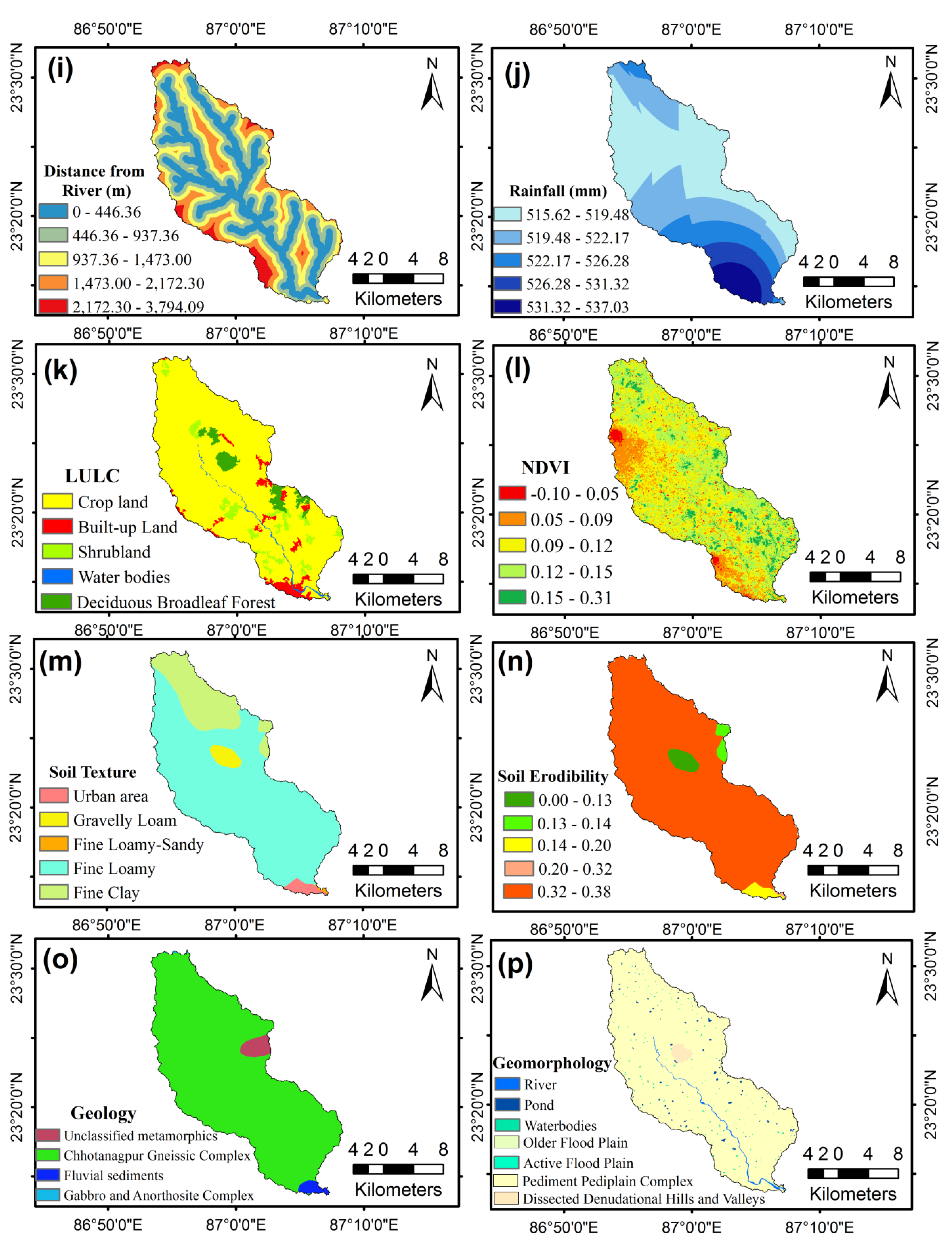
A higher DD represents a highersurface runoff and associated erosional capacity, and vice-versa. The DD is the total length of stream in a particular area. Many factors contribute to the development of DD, including geological structure, soil texture, vegetation coverage, slope etc. The DD was calculated as follows.
D D = i = 1 n S i a
where, i = 1 n S i is the total length of a stream in kilometers and a is total area of the basin in sq. km. The DD value map of the study area was classified into the classes of 0 to 0.66, 0.66 to 1.87, 1.87 to 3.09, 3.09 to 4.35 and 4.35 to 6.73 (km/km2) (Figure 4h).

Distance from River

The drainage system of a watershed is highly correlated with gully head-cut erosion and its retreat. The formation and on-going erosion of a gully head-cut is significantly related to the distance from the river and positively correlated with the drainage system [49]. The Euclidean distance buffering was used to prepare the distance from river map in GIS. The distance from river map is shown in Figure 4i and classified as 0 to 446.36, 446.36 to 937.36, 937.36 to1473, 1473 to 2172.30, 2172.30 to 3794.09 m.

Rainfall

Rainfall is one of the most important factors for GESM. In general, high intensity rainfall and longer rainfall periods cause more intense gully erosion, whereas light rainfall or short duration has less of an effect. After a long dry period, a short but high-intensity rainfall may have high erosive power and facilitate gully formation and erosion. In this study area, we applied the inverse distance weighted (IDW) method to prepare the rainfall map. The rainfall map was classified into the following five categories: 515.62 to 519.48, 519.48 to 522.17, 522.17 to 526.28, 526.28 to 531.32 and 531.32 to 537.03 mm (Figure 4j).

Land Use Land Cover (LULC)

The land use of an area significantly influences on the slope stability and gully formation [50]. Basically, an area covered with dense vegetation is less prone to erosion, whereas an area of barren or sparsely vegetated land is more prone to gully formation and soil erosion. Therefore, LULC is a significant factor in GESM. We used Sentinel 2A satellite data along with a topographic map to prepare the LULC map and determine five LULC types, i.e., crop land, built-up land, shrubland, water bodies and deciduous broadleaf forest (Figure 4k).

Normalized Difference Vegetation Index (NDVI)

The NDVI is widely used to detect the spatio-temporal variation of vegetation cover [51]. It is a measurement of the surface reflectance along with vegetation growth and biomass [52]. Therefore, to understand the vegetation cover and its impact on gully erosion, this factor has been widely used in GESM. The vegetation cover influences erosion through the trees root system, which holds the surrounding soil together. Landsat 8 OLI satellite data was used to calculate the NDVI map using the following equation.
NDVI = ρ N I R ρ R ρ N I R + ρ R
where, ρ N I R is the reflectance of the near infrared band and ρ R is the reflectance of the red band. The NDVI map of the present study area was classified into five classes, i.e., −0.10 to 0.05, 0.05 to 0.09, 0.09 to 0.12, 0.12 to 0.15 and 0.15 to 0.31 (Figure 4l).

Soil Texture

The soil texture of an area plays a vital role on gully erosion as it determines the rate of infiltration, surface and sub-surface runoff, and soil resistance [53]. The soil textures have been used to determine the tunnel erosion or piping, which ultimately form into gullies due to the subsidence of the roofs covering the tunnel. We used the soil texture factor for GESM and has previously also been widely used by several researchers. We classified the study area into the five soil texture units of urban area, gravelly loam, fine loamy sandy, fine loamy, fine clay (Figure 4m).

Soil Erodibility

Soil erodibility largely depends on the soil texture. A sandy, loamy soil texture is more prone to erodibility than gravelly clay loam, for example. Therefore, soil erodibility significantly influences gully erosion, which is why we chose it as a conditioning factor. The soil erodibility map for this area was classified into the classes of 0.00 to 0.13, 0.13 to –0.14, 0.14 to 0.20, 0.20 to 0.32 and 0.32 to 0.38 (Figure 4n).

Geology

The geological structure of an area affects the occurrence of gully erosion. The intensity of weathering largely depends on the geological structures, and it influences the erosional processes. Therefore, it is important to know which rock type is exposed or close to the earth’s surface and potentially influencing gully erosion. In this study area, we found four rock types, namely unclassified metamorphics, the Chotanagpur gneissic complex, fluvial sediments, and the gabbro and anorthosite complex (Figure 4o).

Geomorphology

Geomorphology is the physical features of the earth’s surface and correlates with the geological structures of that area. The erosional pattern of an area is largely dependent on the geomorphological features. Therefore, in this study, we used geomorphology as an important factor for GESM. Seven types of geomorphological features were found on the ISRO’s Geoportal Bhuvan website, and these are river, ponds, water bodies, older flood plain, active flood plain, pediment pediplain complex and dissected denudational hills and valleys (Figure 4p).

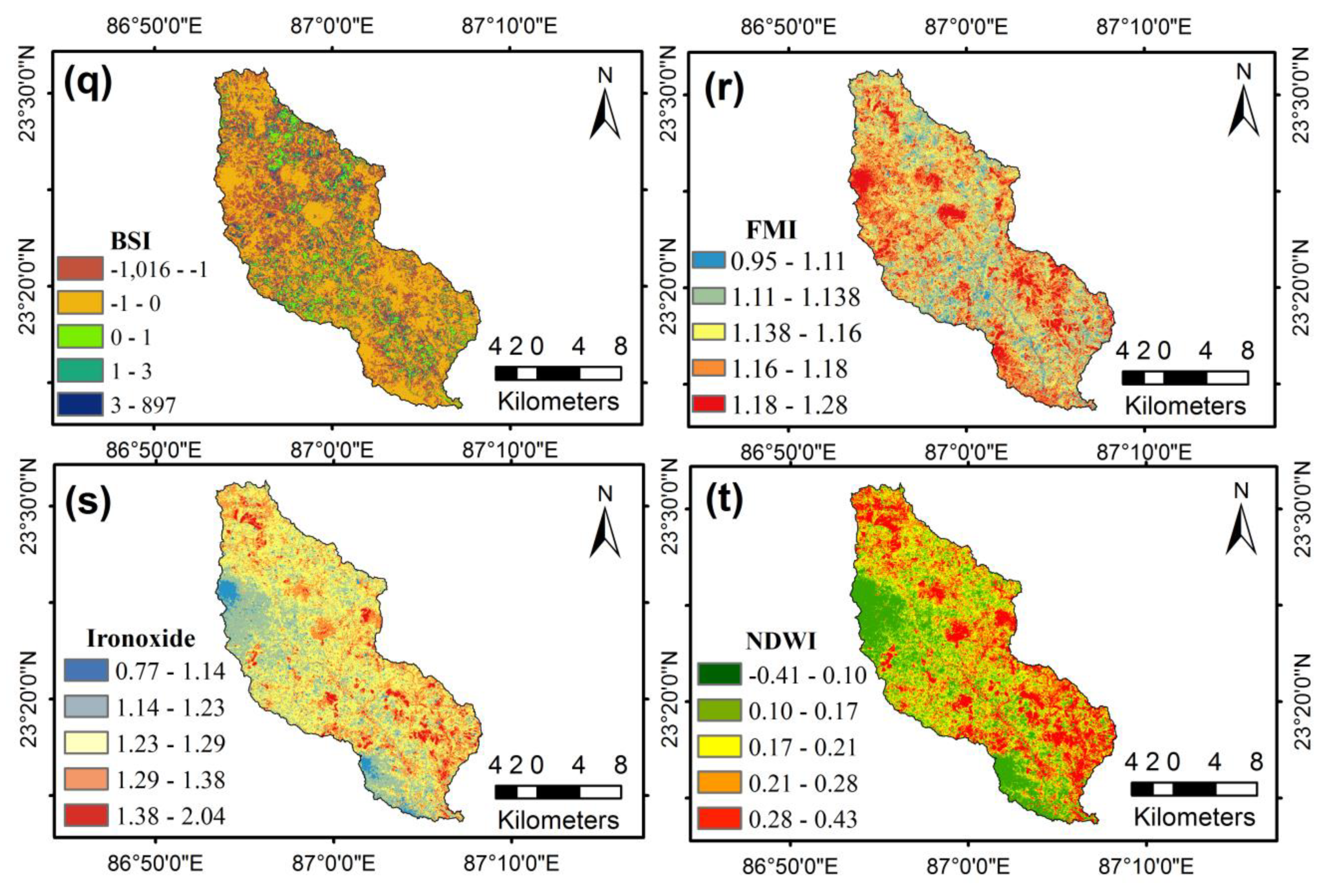
Bare Soil Index (BSI)

The BSI was introduced to differentiate between the bare soil surface from vegetated land area [54]. This index has been widely used to understand the vegetation cover and canopy density of an area [55,56]. We used the BSI as a GECF to evaluate the GESM for better prediction analysis. The following equation was used to obtain the BSI.
B I = ( ρ S W I R + ρ R ) ( ρ N I R + ρ B ) ( ρ S W I R + ρ R ) + ( ρ N I R + ρ B )
where, ρ S W I R represents the reflectance of the short wave infrared band, ρ R represents the reflectance of the red band, ρ N I R represents the reflectance of the near infrared band and ρ B represents the reflectance of the blue band. In our study area, the BSI map value ranges from −1016 to 897 and was classified into five categories (Figure 4q).

Ferrous Minerals Index (FMI)

Ferrous minerals are iron-bearing materials that originate from granite rocks through weathering processes. Basically, this mineral is commonly found in the lateritic soil. In this study, we used FMI as an important GECF for predicting gully susceptibility mapping. The following equation was used to calculate the FMI.
FMI = SWIR NIR
where SWIR is the shortwave infrared band, and NIR is the near infrared band of the electromagnetic spectrum. The FMI map in this study area was classified into the five categories of 0.95 to 1.11, 1.11 to 1.138, 1.138 to 1.16, 1.16 to 1.18 and 1.18 to 1.28 (Figure 4r).

Iron Oxide

Iron oxide is known as ferric oxide, and it is an inorganic compound. Iron oxide is formed through weathering of granitic rocks. Hard outcrops made up of iron minerals are found in lateritic soil. This material indirectly influences erosion through the weathering process. Areas with larger quantities of iron oxide are more susceptible to erosion, and vice-versa. The iron oxide levels in the soil were calculated using the following equation.
Iron   oxide = Red   band Blue   band
The amount of iron oxide in the soil was classified into the five groups of 0.77 to 1.14, 1.14 to 1.23, 1.23 to 1.29, 1.29 to 1.38 and 1.38 to 2.04 (Figure 4s).

Normalized Difference Water Index (NDWI)

The NDWI is used to determine the plant water content. It is essential for understanding the changes in water content and vegetation canopies [57]. In this study, we used the NDWI as a GECF to identify the vegetation health because the state of vegetation health influences the vulnerability to erosion in an area. The NDWI was calculated as follows [57].
N D W I = ρ N I R ρ S W I R ρ N I R + ρ S W I R
where ρ N I R represents the reflectance of the near infrared band and ρ S W I R represents the reflectance of the short wave infrared band. The NDWI map values range from −0.41 to 0.43 (Figure 4t).

2.2.3. Multi-Collinearity (MC) Analysis

The linear relationship between two or more variables in a dataset is known as multi-collinearity [58]. The multi-collinearity analysis is based on the linear dependency among several variables. In general, the MC analysis is carried out when two or more independent variables in a regression model are correlated. The MC analysis indicates a lack of orthogonality among the variables in a dataset. Orthogonal means that there is no linear relationship between the variables [59]. It is well known that even a small MC can create big problems in the dataset and, therefore, prediction results may become inaccurate. Several conditioning factors were used in the GESM. Therefore, it is necessary to identify the perfect relationship among the variables through the MC test. In general, MC occurs when there is a high correlation among the variables in a dataset, in which case it is necessary to remove those particular variables, otherwise, the prediction accuracy will be reduced. In this study, the MC test was carried out using the tolerances (TOL) and variance inflation factors (VIF) techniques. These two techniques were calculated as follows:
T O L = 1 R j 2
V I F = 1 T O L
where R j 2 indicates the regression value of j on added variables in a given dataset. The threshold value of MC occurrence in a dataset is when VIF is >5 and TOL is <0.1.

2.2.4. Importance of GECFs by Random Forest (RF) and SWARA Weight

Random Forest (RF)

The RF is a non-parametric multivariate statistical method. It is a popular ML algorithm which is defined as an ensemble of binary decision trees [60]. This algorithm was developed by Breiman [61] in 2001. Decision trees are incorporated into the RF algorithm by a random selection from the training dataset. During the formation of decision trees, the selection of features is important in the RF algorithm because the RF always tries to choose the most significant features [62]. The decision trees were produced independently during the training phase using the bagging approach [61]. In general, the bagging approach indicates that one sample got chances for more than one time, and others may not for at least one time [63]. The basic function of the RF algorithm is a random vector, i.e., i k , here GECF, is created separately and distributed among all the trees. Thereafter, using the training dataset every tree is grown. Finally, the tree structures of the random vector ( i k ) classifiers represented by h ( X , i k ) , k = 1 , 2 , n are combined for an input vector, i.e., X [64]. In general, the number of decision trees (Ntree) and number of variables (Mtry) are required parameters for RF classifiers [63]. The RF algorithm and its generalization error can be expressed as follows:
G E = P x , y ( m g ( x , y ) < 0 )
m g ( x , y ) = a v k I ( h k ( x ) = y ) m a x j y a v k I ( h k ( x ) = j )
where x and y represent GECFs that specify the probability over the x and y space, m g indicates the marginal function, i.e., the conditional probabilities of the model, and I ( ) represents the indicator function, i.e., described as a set X that indicates the membership of an element in a subset N of X, where the value of 1 indicates all elements of X in N and the value of 0 indicates all elements of X not in N [61]. Furthermore, two types of errors have been calculated in the RF model: The mean decrease in accuracy (MDA) and mean decrease in gini (MDG). The MDA is obtained from the calculation of the out-of-bag (OOB) error, conversely, the MDG is the measurement of the contribution of each variable to the homogeneity of the nodes and leaves. Both MDA and MDG have been used widely in many fields for ranking the variables’ importance and the selection of variables [46,65]. In this study, the average of MDA and MDG has been used to measure the relative importance of gully causative factors, where the OOB error obtained is now 12% so that the model is also 88% accurate to predict the relative important variables.

Step-Wise Weight Assessment Ratio Analysis (SWARA)

Weight assessment is an important technique often applied to solving many problems in different fields of the decision analysis study. In the past few decades, several weight assessment techniques have been developed such as the analytical hierarchy process (AHP) [66], analytical network process (ANP) [67], entropy [68], etc. In 2010, a new multi-criteria decision making method, called SWARA, was introduced. It is a step-by-step weight assessment procedure. In the SWARA approach, an expert opinion is much more important for determining the weights in each criterion. Here, an expert opinion was used to select criteria and rank them based on the experts’ inherent knowledge, experience, information, and understanding. Thus, the most important criterion was given the highest rank, and the least important criterion was given the lowest rank [69]. The weighting parameters were evaluated using the SWARA method [70]. The SWARA method was carried out in the following steps [71,72]:
  • Ordering the criteria based on expert opinion.
  • Endow with relative importance among the criteria.
    An expert gives the importance of the j th criteria with respect to the previous ( j 1 ) criteria according to the average value ( s j ) ratio.
  • Determining the coefficient k j :
    k j = { 1   j = 1 s j + 1   j > 1
  • Computation of the recalculated weight w j :
    w j = { 1   j = 1 x j 1 k j   j > 1
  • Computation of the final weights of the criteria:
    q j = w j k = 1 n w j

2.2.5. Gully Erosion Susceptibility Modelling (GESM)

Boosted Regression Tree (BRT)

The BRT is a ML algorithm that makes use of both statistical and data mining techniques. The main objective of this model is to improve the effectiveness by combining several fitting models [35]. Two different algorithms are used in this model, namely boosting and regression, whereby boosting is used to combine several fitting models, and regression is related to the algorithm of classification and regression tree (CART) class [73]. Boosting is a very dominant ML method for improving the model accuracy, and regression is used to categorize the classification system based on the decision trees group [74,75]. The primary disadvantage of using a single decision tree is that it categorizes the training dataset based on a single tree. Therefore, in this case, there is a probability to loss of information and a very weedy accuracy assessment in the result. Thus, boosting techniques were applied in the BRT model to remove the weakness of the single tree model [76]. Three parameters namely the number of boosting tree iterations, the tree depth interaction, and the shrinkage were used to run the BRT algorithm model [77]. The shrinkage parameter is needed to control the complexity of the model. The tree depth interaction in a BRT model is determined in the course of contributing the trees [78]. The algorithm used in the BRT model can be explained in the following way: BRT is based on prediction variables of X = { x 1 , x n } and the variable of response by y , in which the training sample of { y i , X i } , i = 1 , N of the known y and X values. By analyzing this, a function of F ( X ) is determined that basically maps X to y. According to Friedman [79], of all the values of (y, X), the loss function may be minimized by using the following equation:
F ( X ) = ψ ( y ,   F ( X ) )
The Gradient boosting approximates F ( X ) may be calculated as follows:
F ( X ) = m = 0 M F m ( X ) = m = 0 M β m g ( X ; α m )
where, g ( X ; α m ) represents the regression tree of a particular node, α m represents the tree parameters, and β m represents the coefficients.
Thereafter, the BRT model can be run using the following equation:
F ( X ; [ β m α m ] m 0 ) = m = 0 M β m h ( X ; a m )
where h ( x ; m ) represents the function of a classification with α parameters along with x variables, m represents several stages of the model of variables, and β m represents the coefficient in the stage of m. The BRT model of GESM has been developed using the gbm package in the R statistical software. The gbm.step function was used to fit the model, and the model was simplified by the gbm.simplify function reducing the number of explanatory variables. The BRT also depends on the number of regression trees generated, as in the RF process. Finally, the gully erosion probability was calculated for every pixel of the study area and then the database was formatted to make the map in the Arc GIS environment.

Bayesian Additive Regression Tree (BART)

The framework of the BART model is a nonparametric statistical method that determines the covariates relationship in a dataset. In recent times, this model has performed admirably in the predictive analysis with both continuous and binary datasets. In general, the tree-based ensemble method is used in the BART model, which is basically a Bayesian version of ML techniques [80]. The tree-based ensemble method has an advantage in regression analysis, which isthe fact that this method can fit the nonlinear functional relationship. Therefore, in addition to the aforementioned advantage, the BART model also includes an uncertainty measurement in the prediction results. This model also surpasses several ML algorithms such as random forest, boosting, neural nets, lasso, etc. In this research, we used the BART model to evaluate the reasonable predictive performance along with its uncertainty measurement through prediction intervals [81]. Response variables can be predicted in the BART model by using the Bayesian classification and regression tree (CART) methods [82]. This model also has the capacity to deal with a nonlinear relationship in a variable which is responsible for that model. Furthermore, when irrelevant regression variables are added to this model, it also maintains an excellent predictive result [81]. The following equation can be used to express the BART model:
Y k = j = 1 m g ( x k ; T j , M j ) + ε k
where, Y k represent the tree ensemble model of variables Y, g ( x k ; T j , M j ) is the decision tree of CART, T j is the decision tree j = 1 n (n = sum total number of trees in this model), M j is the parameter of the terminal node of T j , and ε k ~ N ( 0 , σ 2 ) in which, σ 2 is the residual variance.
The Bayesian model is formed by prior distribution in a dataset. Chipman et al. [82] used the following prior distribution to form the Bayesian model:
p ( M 1 , , M n , T 1 , , T n , σ ) [ j i p ( μ i j | T j ) p ( T j ) ] p ( σ )
where, μ i j indicates the parameters of the terminal node of a known tree T j and their prior distribution is represented as follows:
μ i j | T j ~ N ( 0 , σ 0 2 )
where, σ 0 = 0.5 e m and e indicates a hyper-parameter i.e., marginalization of several terminal node parameters.
The combination of Equations (19) and (20) can be used to obtain the posterior distribution of the BART model,
p ( T , M , σ | X , Y ) p ( Y | X , T , M , σ ) × [ j i p ( μ i j | T j ) p ( T j ) ] p ( σ )
where p ( Y | X , T , M , σ ) indicates the likelihood for the sum of trees and T indicates every tree in a given dataset such as T = ( T 1 , . , T n ) . This is obtained by calculating p ( T j | R j , σ ) α p ( T j ) p ( R j ) | T j , σ ) , for accepting and rejecting a new tree from the whole tree system and creating a new set of terminal node parameters for the new tree by applying p ( M j | T j ,   R j , σ ) .
Therefore, the concluding algorithm for the BART model can be described as follows:
p ( R j | T j , σ 2 ) = i = 1 b j + p ( R i j | μ i j , σ 2 ) × p ( μ i j ) p ( σ 2 ) d μ i j .
where R j indicates a vector of partial residuals in this model excluding tree j . In the current work, with the aid of the R programme and R packages, the Bayesian additive regression trees were constructed. This typically results in a complicated decision tree that needs to be “pruned” to express only the most relevant data. The gully and non-gully data have been divided as nominal data, such as 1 and 0, and formed the regression tree for each raster pixel. Thus, the binary predictor of BART was converted into GESM in the Arc GIS environment.

Support Vector Regression (SVR)

The SVR model is a supervised ML algorithm primarily developed by Vapnik et al. [83], and it is widely used by several research groups throughout the world. The SVR algorithm is an adaptation of the newly developed ML algorithm based on support vector machines classification [84]. In general, this model is used to develop structure and control complex functions in a system. Additionally, in a training dataset, the SVR model can maximize the nominal margin through the optimal regression task [85]. The SVR model is generally applied when the dataset is too complex, and this algorithm has the capacity to solve this problem by creating numerous curved margins [86]. In the SVR model, the relationship between input and output variables can be recognized through the structural risk minimization (SRM) norm [87]. Therefore, the calculation of SRM is necessary, and it is done using the following Equations (13) and (14):
y = k ( z ) = v ( z ) + c
where the input data is represented by z = ( z 1 , z 2 , z n ) and the resultant value is represented by y b R l . In addition, v R l indicates the weight factor, c R l indicates the constant number of the mathematical function, and l represents the dataset size in the model. ( z ) indicates the non-linear function to map the input dataset. The following equation can be used to define v and c , and was developed based on the SRM principles:
M i n i m i z e : [ 1 2 | | v | | 2 + P b = 1 1 ( ζ b + ζ b ) ]
S u b j e c t   t o : { y b ( v ( z b ) + c b ) ε + ζ b ( v ( z b ) + c b ) y b ε + ζ b ζ b , ζ b 0
where the penalty factor is P , which balances the model flatness and its risk, ζ b , ζ b indicates slack variables within the model, and ε represents the optimized performance of the model [88]. The Lagrangian function can be used to solve the optimization problem using the following equation:
L ( v , c , ζ b , ζ b , β b , β b , δ b , δ b ) = 1 2 | | v | v | 2 + P b = 1 l ( ζ b + ζ b b = 1 l β b ( ζ b + ε y b + v ( z b z ) + c ) b = 1 l β b ( ζ b + ε + y b v ( z b z ) c ) b = 1 l ( δ b ζ b + ζ b δ b )
In which the Lagrangian multipliers are represented by δ b , δ b , β b   and   β b
Thereafter, SVR can be calculated by:
K ( z ) = b = 1 l ( β b β b ) m ( z , z b ) + c
where the kernel function may be expressed by m ( z , z b ) = ϕ ( z ) ,   ϕ ( z b ) . SVR models require that a vector of real numbers can represent any environmental parameter. The GECFs were derived and converted by GIS into a cell raster. To transfer the grid raster into the data format, an interface program has been developed by LibSVM. The binary classification has only provided the outputs 0 and 1, so we selected the primitive outputs of the core programme for Gaussian distribution.

Bee Algorithm (BA)

The BA was developed to understand the foraging behavior of honeybees, and it is an optimization algorithm generally used to determine the optimal solution [89,90]. The BA considers three kinds of bees, namely the employed bees, onlooker bees, and scout bees. The BA algorithm is completed in five phases, i.e., the phases of initialization, employed bee, onlooker bee, scout bee, and, finally, memorization [91]. The food source information such as the place and amount of food is carried by employed bees to onlooker bees. After that, onlooker bees select the attractive food sources based on nectar contents and fitness, which they calculate. On the other side, scout bees seek new food sources and search several areas. In a nutshell, it can be said that the role of employed and onlooker bees is exploiting while the role of scout bees is exploring [91]. In BA, the possible solution of a problem can be solved through searching for food sources. Here, food sources are D-dimensional vectors in which D represents a number of variables. The fitness of the model is determined by the amount of nectar at a given food source. The following equation is used to calculate the fitness and its limitation:
f = m i n θ i { ( 100 V 1 V 1 V 1 ) 2 + s = 2 S 1 h s ( 50 V h s V 1 ) 2 } ;   i = 1 , 2 , , S  
Subject to,
0 θ i π 2
where V 1 represents the fundamental harmonic, S represents switching the angles number, and h s indicates the S th harmonic variables at the three-phase multilevel output.

Ensemble of SVR and Bee Algorithm

Multiple single models that may be statistical or machine learning have been merged to develop the overall performance, which is known as theensemble approach. In machine learning, the ensemble approach has the capability to improve the prediction accuracy than any single stand-alone model. Thus, keeping in view the advantages of the ensemble approach, it has been widely used for a comprehensive analysis of several hazard-related problems. Several established research works have been used in various ensemble approaches for gully erosion studies with a high prediction accuracy [37,92]. Therefore, in this study, we have also applied the ensemble approach of SVR and the Bee algorithm. Many types of kernel functions were used in the SVR model. In this ensemble model, the Bee algorithm functions have been used instead of the primary kernel function with the SVR model. The ensemble approach in this study was carried out in the ‘R’ statistical programming package, which is freely available and is the most popular software. This ensemble approach is more optimal than the stand-alone machine learning algorithm used in this study for GESM.

2.2.6. Validation and Accuracy Assessment

We carried out a validation and accuracy assessment of several predictive outcomes of the ML models used in this study using the accuracy (ACC) assessment, receiver operating characteristic (ROC) area with the under the curve (AUC), true skill statistic (TSS), and the Kappa coefficient index analysis. All these validation techniques are described in the following section.
The ACC assessment is used to estimate the number of pixels of hazards and non-hazards in an area, in our study, it is used to determine the gully head-cut and non-gully head-cut pixels. The following four indices of true positive (TP), true negative (TN), false positive (FP), and false negative (FN) were used to assess the ACC [93]. Among the aforementioned four indices, TP and FP correctly represented the gully head-cut and non-gully head-cut pixels, while TN and FN incorrectly represented the gully head-cut and non-gully head-cut pixels [94]. The ACC result can be calculated using the equation:
ACC = TP + TN TP + TN + FP + FN
The success of a model, be it a statistical or ML model, can be predicted through the ROC-AUC analysis as it estimates the occurrence and non-occurrence of gully head-cuts on an X and Y axis [93,95], whereby the X axis signifies the sensitivity of the true positive rate (TPR) and the Y axis signifies 1-specificity of the false positive rate (FPR). The sensitivity and 1-specificity were correctly classified as gully head-cuts and non-gully head-cuts susceptibility zones. In a ROC-AUC analysis, training and validation datasets were used to verify the model goodness and prediction ability, respectively [96]. The lower and higher values of a ROC-AUC analysis are 0.5 and 1, whereby the lower (0.5) value indicates poor performance and the higher (1) value indicates a very good performance of the model. The ROC-AUC can be calculated by:
TPR = TP TP + FN
FPR = TN FP + TN
AUC = (   TP +   TN ) ( P + N )
where P and N represent the presence and absence of gully head-cuts, respectively.
TSS is a statistical threshold dependent assessment matrix [97]. This validation method is based on the equal proportions of the events and non-events phenomenon in a validation dataset. The value of TSS ranges from +1 to −1, whereby +1 represents a good performance of the model and a value of less than zero indicates a poor performance of the model. TSS was estimated by:
TSS = TPR FPR
The reliability of several ML models used in GESM was validated through the Kappa coefficient index. When the Kappa value is close to −1, then the model is unreliable, and if the Kappa value is close to +1, then the model is reliable. In this model, the relationship between the estimated and observed values is poor when the Kappa value is <0 [98]. The overall Kappa value ranges can be divided into the following five groups: Slight (0–0.2), fair (0.2–0.4), moderate (0.4–0.6), substantial (0.6–0.8), and conditions (0.8–1) [99]. The following equation was used to calculate the Kappa coefficient index:
Kappa = P a P e x p 1 P e x p
P a = TP + TN TP + TN + FN + FP
P e x p = ( TP + FN ) ( TP + FP ) + ( FP + TN ) ( FN + TN ) ( TP + TN + FN + FP )

3. Results

3.1. Multi-Collinearity Analysis

To stay within the VIF and TOL limit, the 20 gully causative factors that showed no MC were selected and the three variables (distance to road, topographic ruggedness index, and distance from fault) that had co-linearity problems were removed. The selected variables and their multi-collinearity results are shown in Table 2. The ranges of the TOL of the selected variables are 0.244 to 0.886, and the maximum and minimum VIF are 4.16 and 1.12, which indicate no multi-collinearity between the conditioning factors of gully erosion.

3.2. Exploratory Data Analysis

A total of 20 gully formation variables were scrutinized for this gully erosion susceptibility modelling. Each variable was filtered by the multi-collinearity analysis. Figure 5 presents the association between the training dataset (gully and non-gully data) and each variable. The slope mainly varies between 0 and 43 degrees in the Gandheswari watershed, but the gully locations are mainly located in the under 5-degree slope areas. The north, northeast, east, and southeast slope direction are the most prone to gully erosion. There is a significant effect of the topographic elevation on gully erosion, whereby the moderate elevation of 11 to 141 m was found to have the highest concentration of gullies. The flat profile curvature with low convex and concave (0 to 0.8 and −0.8) slope areas is also associated with gully locations. In terms of the plan curvature, about 50% of the training gully locations belong to the flat to slightly convex or concave plan curvature (0 to 1.28 and −1.28). Although the TWI ranges from 7 to 28, 90% of the gully locations lie within the TWI range of 9 to 18. The low to medium (2 to 10) SPI is associated with most of the gully locations. The 48 training gully locations are located in the very low drainage density (0 to 1 km2) regions, and the rest of the gullies fall into the 1 to 4 sq. km drainage densities. Most of the gullies are found near the river, and the gullies slowly decrease with the increasing distance to the drainages. Being a small watershed, the variation of rainfall is a minute and gullies are found in the different rainfall ranges, but a low rainfall is mostly associated with gully locations. The NDVI value of 0.06 to 0.17 is found at about 80% of the gully locations, which means that the sparse vegetation areas are strongly associated with gully erosion. The moderate iron oxide (1.2 to 1.3), FMI (1.10 to 1.23), NDWI (0.06 to 0.24), and BSI (−5 to 9) areas of the watershed were found to contain most of the gullies. The severe soil erodibility (0.24 to 0.39) areas have most of the gullies. The qualitative variables of gully erosion are geology, geomorphology, LULC, and soil texture. The Gandheswari watershed is mainly situated on the geological formation of the Chotanagpur gneissic complex, and all the gullies were found in this formation. Ninety-six percent of the gullies were found in the geomorphological unit of the pediment pediplain complex. In addition, the cropland and the gravelly loam soil textural class are associated with most of the gully locations.

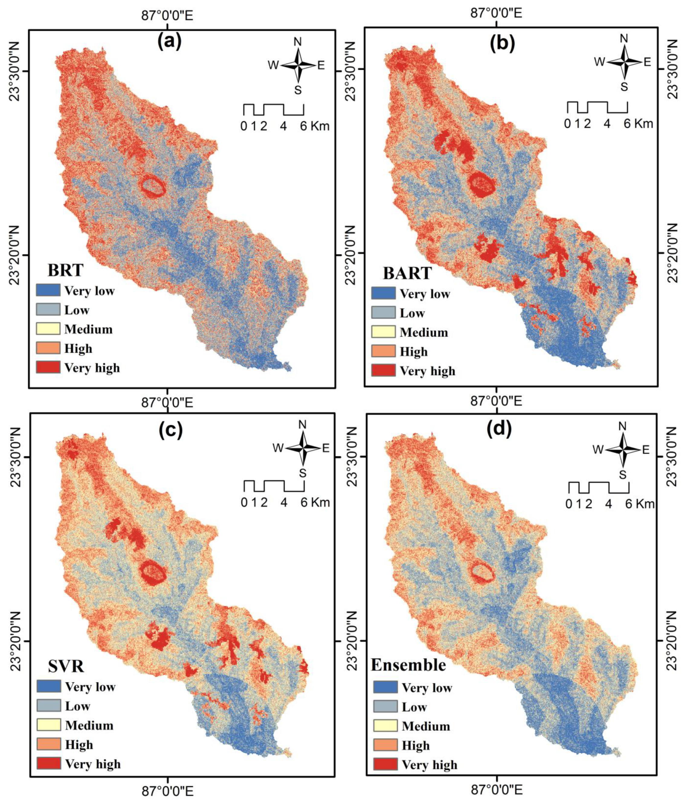
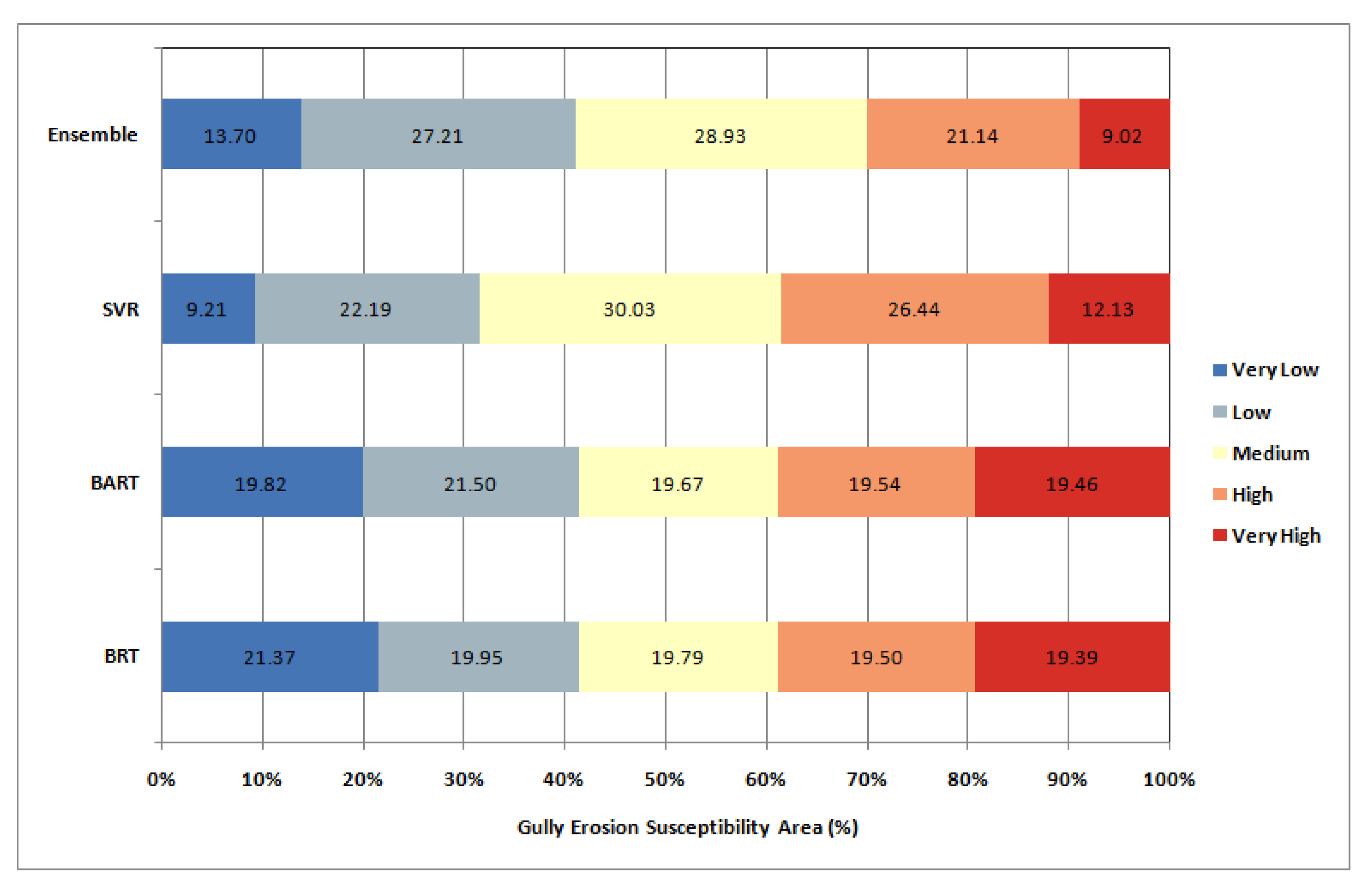
3.3. Spatial Mapping of Gully Erosion Susceptibility

Gully erosion susceptibility maps were created by applying the machine learning and the ensemble models for the Gandheswari watershed. The gully erosion susceptibility maps from all the mentioned models are presented in Figure 5. The maps have been divided into five different susceptibility zones using the natural break methods, and the same symbol is used for each zone of maps. These are veryhigh, high, medium, low, and verylow. All the models have shown consistency between the different susceptibility zones in the four models. The coverage of the very high, high, medium, low, and very low gully erosion susceptibility areas of the BRT model are 21.37, 19.95, 19.79, 19.50, and 19.39% (Figure 6a and Figure 7). The coverage of the very high, high, medium, low, and very low gully erosion susceptibility areas in the BART model are 19.82, 21.50, 19.67, 19.54, and 19.46% (Figure 6b and Figure 7). The BRT and BART model showed more or less the same areal coverage of the gully erosion susceptibility zones. In the case of the SVR model, the coverage for very high, high, medium, low, and very low susceptibility areas are 9.21, 22.19, 30.03, 26.44, and 12.13%, respectively (Figure 5c and Figure 7). The maximum portion of the gully erosion susceptibility area are occupied by the medium and high zone, while the very low and very high zones are occupied by the small portion of the study area. In the ensemble model, the coverage of the very low, low, medium, high, and very high gully erosion susceptibility areas is 13.70, 27.21, 28.93, 21.14, and 9.02%, respectively (Figure 6d and Figure 7). In addition, the maximum portion of the study area is occupied by the low, medium, and high susceptible zones. All the maps showed the upper part of the watershed to be highly susceptible to gully erosion, while the southern part and the mouth of the basin indicated low gully erosion susceptibility.

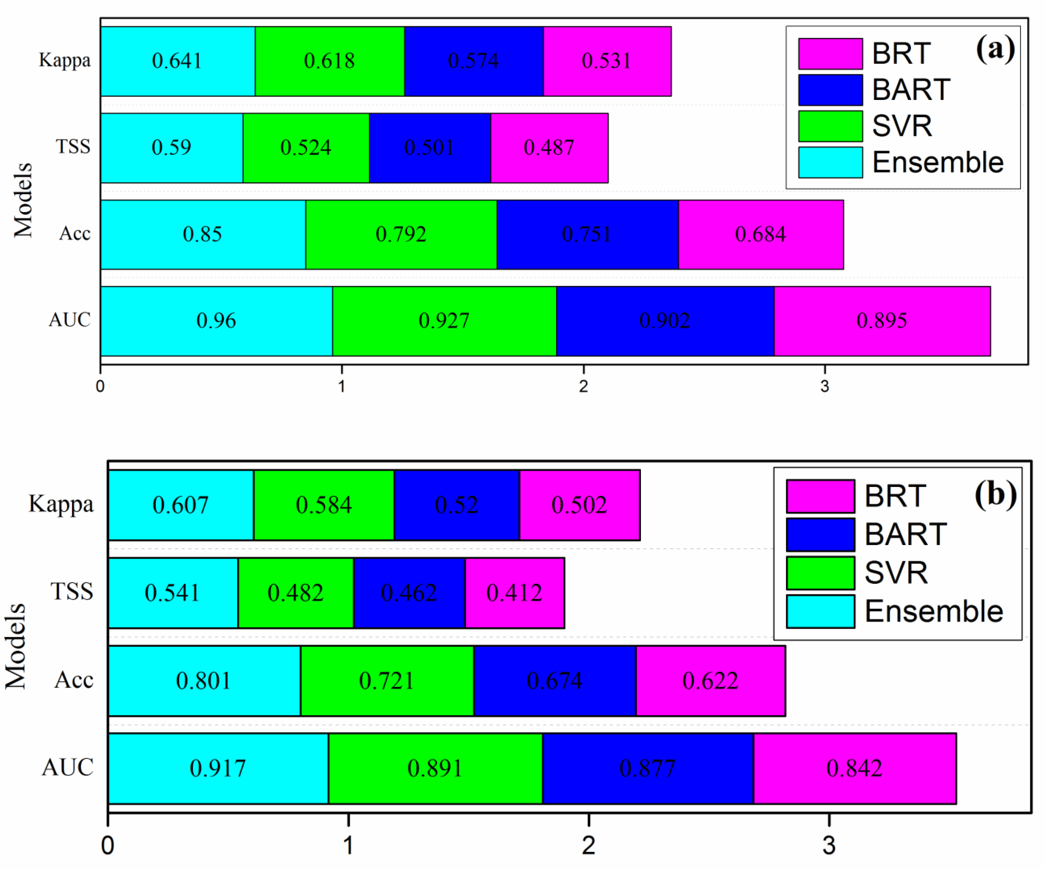
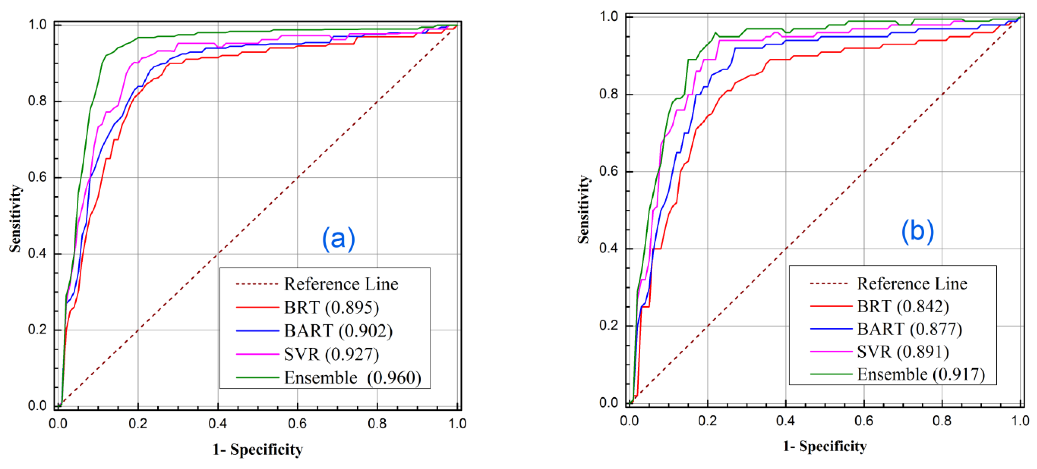
3.4. Model Evaluation Performance Result

The AUC ranges from 0.5 to 1, whereby values closer to 0.1 indicate that the model has provided a perfect prediction, while values closer to 0.5 indicate that there is a problem with model fitting. Other model diagnostic tools such as Acc, TSS, and Kappa have also been used to find a suitable robust gully erosion susceptibility model (Figure 8). In this study, the models were evaluated by both the training and validation datasets of gully and non-gully locations to measure the success and prediction performance of the model. The evaluation result of the model performances in the training stage and testing stage for all the machine learning and the ensemble model are summarized in Figure 8. All the evaluation results indicated that the BAR, BART, SVR, and ensemble models perform well and that the data were sufficient for training and validating the gully data. The ensemble model is the most robust model in this study and yielded the highest AUC, Acc, TSS, and Kappa in the training (AUC, 0.960; Acc, 0.850; TSS, 0.590; Kappa, 0.641) and validation stage (AUC, 0.917; Acc, 0.801; TSS, 0.607; Kappa, 0.541). The AUC value of the ensemble model when considering the gully training points is 0.960, which indicates a high success capacity. The rest of the models also yielded the optimal accuracy, coming close to that of the ensemble model. The AUC of the SVR, BART, and BRT is 0.927, 0.902, and 89.5, respectively (Figure 9a). When we considered the validation dataset, the prediction rate capacity of ROC indicates the same trend of model robustness (Figure 9b). The values of Acc in the ensemble, SVR, BART, and BRT for the training datasets are 0.85, 0.792, 0.751, and 0.684 and the Acc values for the validation datasets are 0.801, 0.721, 0.674, and 0.622, respectively. The evaluation results of TSS and Kappa also showed the same trend of AUC and Acc in the training and testing stage. Therefore, it can be concluded that both predictions, the (testing dataset) and success (training dataset) rate showed little variation of results and a good accuracy of the models, which were deemed to produce realistic and accurate gully erosion susceptibility maps for delineating the gully erosion areas.
Figure 10 shows the two-dimensional graphical presentation of the observed gully erosion and the predictive gully erosion susceptibility for the BRT, BART, SVR, and ensemble models on a Taylor diagram. The diagram summarizes the multiple statistical aspects of the model performance in a single diagram (Taylor, 2001). The Taylor diagram represents the connection between the predicted and observed gully erosion in the Gandheswari watershed. All the machine learning and the ensemble models are similar in their ability to predict the gully erosion, but the ensemble models yielded the highest correlation and lowest standard deviation. Therefore, the ensemble gully erosion susceptibility model is the most robust model.

3.5. Relative Importance of the Variables

The predisposing factors of gully erosion susceptibility modelling have been selected by considering the various available literature and physical characteristics of the study area, and then the multi-collinearity analysis for these factors was carried out. The assessment of important variables of gully erosion was done through the mean decrease accuracy, using the RF model, as shown in Table 3. The high mean decrease in accuracy represents the high importance of the input variables of the gully erosion susceptibility in this RF calculation. According to Table 3, the most important variables for the formation and development of gullies in this basin are the NDVI (22.62) followed by plan curvature (20.24). The other relative important factors of gully formation are SPI (16.48), geology (15.41), drainage density (14.51), geomorphology (13.21), and elevation (10.02). The relative importance value showed a strong relationship between the above parameters and gully erosion. On the other hand, the iron oxide (0.42), FMI (0.94), TWI (1.13), aspect (1.32), profile curvature (1.49), NDWI (1.76), and BSI (1.84) are the least significant variables in terms of gully erosion. In addition, the rest of the variables, i.e., rainfall (8.68), slope (7.51), LULC (5.42), soil texture (3.24), distance to river (3.06), and soil erodibility (2.13) are moderately important variables.

3.6. Relative Importance of Sub-Classes of the Variables

Many gully erosion susceptibility studies showed only the assessment of important variables affecting gully erosion, but it is also significant to identify the sub-factors or sub-classes of each conditioning factor of gully erosion. The relationships of gully erosion with each sub-factor of gully conditioning factors were obtained from the SWARA weight analysis and are shown in Table 4. The SWARA weights of the sub-factors of each conditioning factor show that the high (5.75 to 15.24) slope areas are associated with a higher weight (0.41) and very likely prone to gully erosion. A very high slope (15.24 to 43.18) was not associated with gully formation, but the weight decreased with medium to very low slope areas. In terms of the aspect, all directions of the slope are associated with gully formation except the flat (0.05), west (0.06), and northeast (0.06) slope directions. The medium elevation class (80 to 141 m) was weighted as 0.61, which means it is strongly associated with the occurrence of gullies in the study area. Higher (0.28 to 0.84) classes of profile curvature are associated with an increased likelihood to affect gully erosion based on the weighting of 0.40. The five classes of plan curvature are associated with a high probability to affect gully formation, and the very high (0.86 to 2.96) class has the highest weight (0.36). High classes of TWI (14.05 to 17.24) and SPI (7.57 to 10.69) are associated with the maximum probability of gully erosion, and the weights of the components are 0.41 and 0.52, respectively. The very low drainage density (0 to 0.66 km/sq.km) class has a very high (0.36) probability of gully erosion, while the highest class of distance to the river (2172.30 to 3794.09 m) has a high SWARA weight (0.43). A low and medium rainfall (515.62 to 522.17 mm) is most favorable for gully formation, and gully erosion and the weights of the two classes are 0.37 and 0.39, respectively. The shrubland areas are prone to gully erosion because shrubland is often associated with barren land and the SWARA weight of the shrubland is 0.56. The NDVI is the most important factor affecting gully erosion, and in our study area, the NDVI ranges from −0.10 to 0.31 with the very high class being the most favorable to gully erosion with a weight of 0.34. Most of the area (96% of the study area) is covered by the Chotanagpur gneissic complex geological formation, so this geological formation has received the highest weight. The gravelly loam soil texture group with very low soil erodibility (0.00–0.13) has high weights (0.42 and 0.79), meaning that these areas are most favorable for gully erosion. Therefore, the dissected denudational hills and valleys are an effective geomorphological unit for probable gully erosion. Accordingly, low to very high FMI (0.95 to 1.28) and high to very high (1.29 to 2.04) iron oxide classes are considered being more favorable to gully erosion. The medium BSI covers 99% of the study area, so this class automatically receives the highest weight (1.0). The low NDWI (−0.41 to 0.10) class received a higher SWARA weight (0.31), so it is associated with gully erosion.

4. Discussion

The gully erosion susceptibility assessment is crucial for the preparation of erosion control and mitigation measures [100]. To obtain reliable and highly accurate maps of gully erosion susceptibility is a challenge for planners and managers [101]. To overcome the challenges, researchers have tried to propose novel susceptibility models and tested them in gully prone regions around the world. Different approaches, procedures, and models for the spatial prediction of natural hazards and disasters have been developed, and these models have been implemented around the world. The aims of all these methods are the same in all approaches [41]. For the past decades, many statistical and heuristic susceptibility methods have been used to understand different environmental hazards [38,102,103]. However, these above-mentioned susceptibility models have some limitations in their ability to analyze the multifarious connection between predictors and response, and, very recently, data mining/machine learning ensemble models have been developed for gully erosion susceptibility modelling [48,104,105]. In this paper, we proposed and evaluated three machine learning models and one ensemble model for gully erosion susceptibility modelling with the highest possible precision and suggested the most suitable model for the Gandheswari watershed. The proposed models are the BRT, BART, SVR, and the ensemble model of the Bee and SVR algorithm. Prediction, categorization, clustering, and elaboration of environmental hazards’ data were assessed in the application of the machine learning approaches [41,106].
Gully erosion is controlled by several geo-environmental factors [107]. Therefore, the variables of the gully erosion susceptibility modelling have been incorporated based on suggested approaches in similar published research and the geo-environmental characteristics of the study area. The topographic, hydrological, geological, and anthropogenic (land use) attributes are the most important variables for the development of gullies around the world [107,108,109].
The spatial resolution of the input variables greatly affects the output result, and many topographical factors were derived from the DEM. We used a 12.5 m spatial resolution ALOS PALSAR DEM [109]. We selected the 20 individual gully conditioning factors based on the outcome of the multi-collinearity assessment. The multi-collinearity assessment of factors based on the TOL and VIF is the best method to check for a collinearity between the variables because this multi-collinearity check can increase the accuracy of the model [23]. According to the relative importance variables based on the mean decrease accuracy (MDA), the NDVI is the most important factor followed by the plan curvature. Other factors such as SPI, geology, drainage density, geomorphology, and elevation are responsible for gully erosion in this watershed. We examined the various available literature regarding the gully erosion susceptibility model and previous authors suggest that the relative importance of conditioning factors for gully erosion are area-specific and are thus, not transferable to other regions [100]. For some examples from eastern India, Saha et al. [41] identified the elevation, rainfall, NDVI, LULC, and slope as the most important factors, whereas Gayen et al. [110] reported that the LULC, drainage density, elevation, soil type, and distance from lineament are the most effective factors contributing to gully erosion. The SWARA weight is one of the methods used to define the weight of the sub-classes of the factors that play a dominant role in the modelling process [69]. The role of each individual class of each causal gully erosion factor is shown in Table 4.
To analyze the multifunction connection between the response (gully) and the predictors (gully conditioning factors), machine learning ensemble approaches were used for their ability to produce robust gully erosion susceptibility models [91]. The BRT models used two algorithms, i.e., boosting and regression, and, in this study, we used it for the spatial prediction of the gully erosion, but it has also been applied for many environmental hazards. Zabihi et al. [111] found that the BRT model is better for gully erosion susceptibility than the multivariate adaptive regression spline (MARS) model.BART, which is a newly invented tree classifier approach, provides admirable performance in both binary and continuous datasets and was successfully applied in this study [112]. The other interesting supervised machine learning algorithm is SVR, which is widely used in many susceptibility models, such as landslide susceptibility and groundwater potentiality [36,113]. In this study, the SVR model successfully predicts gully erosion. We applied the Bee algorithm with the SVR model and established a novel ensemble model, which yielded the best accuracy compared to the gully erosion susceptibility models based on the three stand-alone machine learning algorithms.
Furthermore, to compare the performance and robustness of the model, several researchers applied the AUC of ROC curve, accuracy, TSS, and Kappa index [37,38,39]. Each gully susceptibility model was evaluated by the above model evaluator in the training and testing stage. The results demonstrated that all the models performed well, but that the ensemble models have provided the best prediction of gully erosion. Several gully erosion susceptibility studies found that the ensemble algorithm of the machine learning model is the most suitable model [18,114]. A previous gully erosion susceptibility study in the Gandheswari watershed indicates that the multi-layer perception approach (MLPC) and its ensembles (MLPC-Bagging, MLPC-Dagging, and MLPC-Decorate) yielded the best result, but that the MLPC-Decorate is the best ensemble model with an AUC of ROC curve of 0.906 [23].

5. Conclusions

Various types of soil erosion processes can accelerate land degradation, and have a negative impact on agriculture. There are various types of soil erosion processes occurring at the surface, which are sheet erosion, rills, gullies, ravines, etc. Globally, gully erosion, or the development of gullies, is one of the most destructive processes of land degradation. In this study, the objective was the gully erosion susceptibility modelling and mapping for the Gandheswari watershed. Stand-alone and ensemble classifier models with gully inventory datasets and gully conditioning factors were successfully used to assess the gully erosion susceptibility. The AUC of ROC curve, accuracy, TSS, and Kappa index were employed to assess and compare the gully erosion susceptibility models. The results of the model evaluation from the training and validation gully inventory datasets have shown that the gully susceptibility models prepared based on the BRT, BART, SVR, and ensemble approaches performed best in terms of fitting and the prediction capability of the model. The output susceptibility maps and the model performance evaluation result indicate that the ensemble of the SVR-Bee model is the best-fit model, and it is most capable of predicting the occurrence of gullies in the study area. The relative importance result of the gully causative factors and their sub-classes showed that the NDVI and plan curvature are the most important factors. All four gully erosion susceptibility maps reveal a good consistency between the spatial zones of the different susceptibilities of gully erosion. Furthermore, the most valuable outcomes of the study are the gully susceptibility maps, which will help the local administrators, decision-makers, and planners manage land degradation and land use planning. In addition, the new susceptibility methods may help further research addressing various environmental hazards such as landslides, flooding, and soil erosion. Since no study is without any limitations, we need to emphasize that this study has not included the full hydrological modelling of gully systems, which is a challenging task for future studies.

Author Contributions

Conceptualization, I.C., S.C.P., and A.A.; methodology, I.C., S.C.P., and A.A.; software, I.C., S.C.P., and A.A.; validation, I.C., S.C.P., A.S., and A.A.; formal analysis, I.C., S.C.P., and A.A.; investigation, I.C., S.C.P., A.A., and R.C.; resources, I.C., S.C.P., and A.A.; data curation, I.C., S.C.P., and A.A.; writing—original draft preparation, I.C., S.C.P., A.S., B.P., R.C., and A.A.; writing—review and editing, I.C., S.C.P., A.S., B.P., R.C., A.A., T.B., and S.S.B.; supervision, A.A. and T.B.; funding acquisition, T.B. All authors have read and agreed to the published version of the manuscript.

Funding

Open Access was funded by the Austrian Science Fund (FWF) through the Doctoral College GIScience (DK W 1237-N23) at the University of Salzburg.

Acknowledgments

Open Access Funding by the Austrian Science Fund (FWF).

Conflicts of Interest

The authors declare no conflict of interest.

References

  1. Billi, P.; Dramis, F. Geomorphological investigation on gully erosion in the Rift Valley and the northern highlands of Ethiopia. Catena 2003, 50, 353–368. [Google Scholar] [CrossRef]
  2. Saha, A.; Ghosh, M.; Pal, S.C. Understanding the Morphology and Development of a Rill-Gully: An Empirical Study of Khoai Badland, West Bengal, India. In Gully Erosion Studies from India and Surrounding Regions; Springer International Publishing: Cham, Switzerland, 2020; pp. 147–161. [Google Scholar]
  3. Lal, R. Offsetting global CO2 emissions by restoration of degraded soils and intensification of world agriculture and forestry. Land Degrad. Dev. 2003, 14, 309–322. [Google Scholar] [CrossRef]
  4. Poesen, J.; Nachtergaele, J.; Verstraeten, G.; Valentin, C. Gully erosion and environmental change: Importance and research needs. Catena 2003, 50, 91–133. [Google Scholar] [CrossRef]
  5. Valentin, C.; Poesen, J.; Li, Y. Gully erosion: Impacts, factors and control. Catena 2005, 63, 132–153. [Google Scholar] [CrossRef]
  6. Imeson, A.C.; Kwaad, F.J.P.M.; Mucher, H.J. Hillslope processes and deposits in forested areas of Luxembourg. In Timescales in Geomorphology; John Wiley and Sons Ltd.: Hoboken, NJ, USA, 1980; pp. 31–42. [Google Scholar]
  7. Poesen, J. Soil erosion in the Anthropocene: Research needs. Earth Surf. Process. Landf. 2018, 43, 64–84. [Google Scholar] [CrossRef]
  8. Ghosh, S.; Guchhait, S.K. Geomorphic threshold estimation for gully erosion in the lateritic soil of Birbhum, West Bengal, India. Soil Discuss. 2016, 1–29. [Google Scholar] [CrossRef] [Green Version]
  9. Sinha, D.; Joshi, V.U. Application of Universal Soil Loss Equation (USLE) to recently reclaimed badlands along the Adula and Mahalungi Rivers, Pravara Basin, Maharashtra. J. Geol. Soc. India 2012, 80, 341–350. [Google Scholar] [CrossRef]
  10. Bhattacharyya, T.; Babu, R.; Sarkar, D.; Mandal, C.; Dhyani, B.L.; Nagar, A.P. Soil loss and crop productivity model in humid subtropical India. Curr. Sci. 2007, 93, 1397–1403. [Google Scholar]
  11. Sharda, V.N.; Dogra, P.; Prakash, C. Assessment of production losses due to water erosion in rainfed areas of India. J. Soil Water Conserv. 2010, 65, 79–91. [Google Scholar] [CrossRef]
  12. Kachouri, S.; Achour, H.; Abida, H.; Bouaziz, S. Soil erosion hazard mapping using Analytic Hierarchy Process and logistic regression: A case study of Haffouz watershed, central Tunisia. Arab. J. Geosci. 2015, 8, 4257–4268. [Google Scholar] [CrossRef]
  13. Achour, Y.; Boumezbeur, A.; Hadji, R.; Chouabbi, A.; Cavaleiro, V.; Bendaoud, E.A. Landslide susceptibility mapping using analytic hierarchy process and information value methods along a highway road section in Constantine, Algeria. Arab. J. Geosci. 2017, 10, 194. [Google Scholar] [CrossRef]
  14. Kheir, R.B.; Wilson, J.; Deng, Y. Use of terrain variables for mapping gully erosion susceptibility in Lebanon. Earth Surf. Process. Landf. 2007, 32, 1770–1782. [Google Scholar] [CrossRef]
  15. Arabameri, A.; Rezaei, K.; Pourghasemi, H.R.; Lee, S.; Yamani, M. GIS-based gully erosion susceptibility mapping: A comparison among three data-driven models and AHP knowledge-based technique. Environ. Earth Sci. 2018, 77, 628. [Google Scholar] [CrossRef]
  16. Azareh, A.; Rahmati, O.; Rafiei-Sardooi, E.; Sankey, J.B.; Lee, S.; Shahabi, H.; Ahmad, B.B. Modelling gully-erosion susceptibility in a semi-arid region, Iran: Investigation of applicability of certainty factor and maximum entropy models. Sci. Total Environ. 2019, 655, 684–696. [Google Scholar] [CrossRef] [PubMed]
  17. Arabameri, A.; Cerda, A.; Tiefenbacher, J.P. Spatial Pattern Analysis and Prediction of Gully Erosion Using Novel Hybrid Model of Entropy-Weight of Evidence. Water 2019, 11, 1129. [Google Scholar] [CrossRef] [Green Version]
  18. Arabameri, A.; Pradhan, B.; Rezaei, K.; Yamani, M.; Pourghasemi, H.R.; Lombardo, L. Spatial modelling of gully erosion using evidential belief function, logistic regression, and a new ensemble of evidential belief function-logistic regression algorithm. Land Degrad. Dev. 2018, 29, 4035–4049. [Google Scholar] [CrossRef]
  19. Band, S.S.; Janizadeh, S.; Chandra Pal, S.; Saha, A.; Chakrabortty, R.; Shokri, M.; Mosavi, A. Novel Ensemble Approach of Deep Learning Neural Network (DLNN) Model and Particle Swarm Optimization (PSO) Algorithm for Prediction of Gully Erosion Susceptibility. Sensors 2020, 20, 5609. [Google Scholar] [CrossRef]
  20. Arabameri, A.; Yamani, M.; Pradhan, B.; Melesse, A.; Shirani, K.; Tien Bui, D. Novel ensembles of COPRAS multi-criteria decision-making with logistic regression, boosted regression tree, and random forest for spatial prediction of gully erosion susceptibility. Sci. Total Environ. 2019, 688, 903–916. [Google Scholar] [CrossRef]
  21. Arabameri, A.; Pradhan, B.; Lombardo, L. Comparative assessment using boosted regression trees, binary logistic regression, frequency ratio and numerical risk factor for gully erosion susceptibility modelling. Catena 2019, 183, 104223. [Google Scholar] [CrossRef]
  22. Arabameri, A.; Chen, W.; Loche, M.; Zhao, X.; Li, Y.; Lombardo, L.; Cerda, A.; Pradhan, B.; Bui, D.T. Comparison of machine learning models for gully erosion susceptibility mapping. Geosci. Front. 2020, 11, 1609–1620. [Google Scholar] [CrossRef]
  23. Roy, P.; Chakrabortty, R.; Chowdhuri, I.; Malik, S.; Das, B.; Pal, S.C. Development of Different Machine Learning Ensemble Classifier for Gully Erosion Susceptibility in Gandheswari Watershed of West Bengal, India. Mach. Learn. Intell. Decis. Sci. 2020, 1–26. [Google Scholar] [CrossRef]
  24. Chen, W.; Panahi, M.; Khosravi, K.; Pourghasemi, H.R.; Rezaie, F.; Parvinnezhad, D. Spatial prediction of groundwater potentiality using ANFIS ensembled with teaching-learning-based and biogeography-based optimization. J. Hydrol. 2019, 572, 435–448. [Google Scholar] [CrossRef]
  25. Ghosh, S.; Guchhait, S.K. Estimation of geomorphic threshold in permanent gullies of lateritic terrain in Birbhum, West Bengal, India. Curr. Sci. (00113891) 2017, 113, 478–485. [Google Scholar] [CrossRef]
  26. Hembram, T.K.; Saha, S. Prioritization of sub-watersheds for soil erosion based on morphometric attributes using fuzzy AHP and compound factor in Jainti River basin, Jharkhand, Eastern India. Environ. Dev. Sustain. 2020, 22, 1241–1268. [Google Scholar] [CrossRef]
  27. Chakrabortty, R.; Pal, S.C.; Chowdhuri, I.; Malik, S.; Das, B. Assessing the Importance of Static and Dynamic Causative Factors on Erosion Potentiality Using SWAT, EBF with Uncertainty and Plausibility, Logistic Regression and Novel Ensemble Model in a Sub-tropical Environment. J. Indian Soc. Remote Sens. 2020, 48, 1–25. [Google Scholar] [CrossRef]
  28. Chakrabortty, R.; Pal, S.C.; Sahana, M.; Mondal, A.; Dou, J.; Pham, B.T.; Yunus, A.P. Soil erosion potential hotspot zone identification using machine learning and statistical approaches in eastern India. Nat. Hazards 2020, 104, 1259–1294. [Google Scholar] [CrossRef]
  29. Ghosh, D.; Mandal, M.; Karmakar, M.; Banerjee, M.; Mandal, D. Application of geospatial technology for delineating groundwater potential zones in the Gandheswari watershed, West Bengal. Sustain. Water Resour. Manag. 2020, 6, 14. [Google Scholar] [CrossRef]
  30. Chakrabortty, R.; Pal, S.C.; Malik, S.; Das, B. Modeling and mapping of groundwater potentiality zones using AHP and GIS technique: A case study of Raniganj Block, Paschim Bardhaman, West Bengal. Model. Earth Syst. Environ. 2018, 4, 1085–1110. [Google Scholar] [CrossRef]
  31. Das, B.; Nandy, M. Tectono-stratigraphic studies of the supra-crustal rocks at the southern contact of the Chhotanagpur Granite Gneiss with Proterozoic Mobile Belt in Bankura and Purulia districts West Bengal. Rec. Geol. Surv. India 1997, 129 Pt 3. [Google Scholar]
  32. Shit, P.K.; Nandi, A.S.; Bhunia, G.S. Soil erosion risk mapping using RUSLE model on jhargram sub-division at West Bengal in India. Model. Earth Syst. Environ. 2015, 1, 28. [Google Scholar] [CrossRef] [Green Version]
  33. Shit, P.K.; Maiti, R.K. Mechanism of Gully-Head Retreat—A Study at Ganganir Danga, Paschim Medinipur, West Bengal. Ethiop. J. Environ. Stud. Manag. 2012, 5, 332–342. [Google Scholar] [CrossRef] [Green Version]
  34. Lay, U.S.; Pradhan, B.; Yusoff, Z.B.M.; Abdallah, A.F.B.; Aryal, J.; Park, H.-J. Data Mining and Statistical Approaches in Debris-Flow Susceptibility Modelling Using Airborne LiDAR Data. Sensors 2019, 19, 3451. [Google Scholar] [CrossRef] [Green Version]
  35. Aertsen, W.; Kint, V.; Van Orshoven, J.; Özkan, K.; Muys, B. Comparison and ranking of different modelling techniques for prediction of site index in Mediterranean mountain forests. Ecol. Model. 2010, 221, 1119–1130. [Google Scholar] [CrossRef]
  36. Panahi, M.; Gayen, A.; Pourghasemi, H.R.; Rezaie, F.; Lee, S. Spatial prediction of landslide susceptibility using hybrid support vector regression (SVR) and the adaptive neuro-fuzzy inference system (ANFIS) with various metaheuristic algorithms. Sci. Total Environ. 2020, 741, 139937. [Google Scholar] [CrossRef]
  37. Arabameri, A.; Chen, W.; Lombardo, L.; Blaschke, T.; Tien Bui, D. Hybrid computational intelligence models for improvement gully erosion assessment. Remote Sens. 2020, 12, 140. [Google Scholar] [CrossRef] [Green Version]
  38. Arabameri, A.; Pradhan, B.; Bui, D.T. Spatial modelling of gully erosion in the Ardib River Watershed using three statistical-based techniques. Catena 2020, 190, 104545. [Google Scholar] [CrossRef]
  39. Pourghasemi, H.R.; Gayen, A.; Haque, S.M.; Bai, S. Gully Erosion Susceptibility Assessment Through the SVM Machine Learning Algorithm (SVM-MLA). In Gully Erosion Studies from India and Surrounding Regions; Springer International Publishing: Cham, Switzerland, 2020; pp. 415–425. [Google Scholar]
  40. Arabameri, A.; Saha, S.; Mukherjee, K.; Blaschke, T.; Chen, W.; Ngo, P.T.T.; Band, S.S. Modeling Spatial Flood using Novel Ensemble Artificial Intelligence Approaches in Northern Iran. Remote Sens. 2020, 12, 3423. [Google Scholar] [CrossRef]
  41. Saha, S.; Roy, J.; Arabameri, A.; Blaschke, T.; Tien Bui, D. Machine Learning-Based Gully Erosion Susceptibility Mapping: A Case Study of Eastern India. Sensors 2020, 20, 1313. [Google Scholar] [CrossRef] [Green Version]
  42. Conforti, M.; Aucelli, P.P.; Robustelli, G.; Scarciglia, F. Geomorphology and GIS analysis for mapping gully erosion susceptibility in the Turbolo stream catchment (Northern Calabria, Italy). Nat. Hazards 2011, 56, 881–898. [Google Scholar] [CrossRef]
  43. Rahmati, O.; Pourghasemi, H.R.; Zeinivand, H. Flood susceptibility mapping using frequency ratio and weights-of-evidence models in the Golastan Province, Iran. Geocarto Int. 2016, 31, 42–70. [Google Scholar] [CrossRef]
  44. Conoscenti, C.; Agnesi, V.; Angileri, S.; Cappadonia, C.; Rotigliano, E.; Märker, M. A GIS-based approach for gully erosion susceptibility modelling: A test in Sicily, Italy. Environ. Earth Sci. 2013, 70, 1179–1195. [Google Scholar] [CrossRef]
  45. Wilson, J.P.; Gallant, J.C. Terrain Analysis: Principles and Applications; John Wiley & Sons: Hoboken, NJ, USA, 2000; ISBN 978-0-471-32188-0. [Google Scholar]
  46. Rahmati, O.; Pourghasemi, H.R.; Melesse, A.M. Application of GIS-based data driven random forest and maximum entropy models for groundwater potential mapping: A case study at Mehran Region, Iran. Catena 2016, 137, 360–372. [Google Scholar] [CrossRef]
  47. Moore, I.D.; Grayson, R.B.; Ladson, A.R. Digital terrain modelling: A review of hydrological, geomorphological, and biological applications. Hydrol. Process. 1991, 5, 3–30. [Google Scholar] [CrossRef]
  48. Kadavi, P.R.; Lee, C.-W.; Lee, S. Application of Ensemble-Based Machine Learning Models to Landslide Susceptibility Mapping. Remote Sens. 2018, 10, 1252. [Google Scholar] [CrossRef] [Green Version]
  49. Conoscenti, C.; Angileri, S.; Cappadonia, C.; Rotigliano, E.; Agnesi, V.; Märker, M. Gully erosion susceptibility assessment by means of GIS-based logistic regression: A case of Sicily (Italy). Geomorphology 2014, 204, 399–411. [Google Scholar] [CrossRef] [Green Version]
  50. Zakerinejad, R.; Maerker, M. An integrated assessment of soil erosion dynamics with special emphasis on gully erosion in the Mazayjan basin, southwestern Iran. Nat. Hazards 2015, 79, 25–50. [Google Scholar] [CrossRef]
  51. Malik, S.; Pal, S.C.; Das, B.; Chakrabortty, R. Assessment of vegetation status of Sali River basin, a tributary of Damodar River in Bankura District, West Bengal, using satellite data. Environ. Dev. Sustain. 2020, 22, 5651–5685. [Google Scholar] [CrossRef]
  52. Wu, Y.; Li, W.; Wang, Q.; Liu, Q.; Yang, D.; Xing, M.; Pei, Y.; Yan, S. Landslide susceptibility assessment using frequency ratio, statistical index and certainty factor models for the Gangu County, China. Arab. J. Geosci. 2016, 9, 84. [Google Scholar] [CrossRef]
  53. Deng, L.; Zeng, G.; Fan, C.; Lu, L.; Chen, X.; Chen, M.; Wu, H.; He, X.; He, Y. Response of rhizosphere microbial community structure and diversity to heavy metal co-pollution in arable soil. Appl. Microbiol. Biotechnol. 2015, 99, 8259–8269. [Google Scholar] [CrossRef]
  54. Abd-El Monsef, H.; Smith, S.E. A new approach for estimating mangrove canopy cover using Landsat 8 imagery. Comput. Electron. Agric. 2017, 135, 183–194. [Google Scholar] [CrossRef]
  55. Malik, S.; Pal, S.C.; Das, B.; Chakrabortty, R. Intra-annual variations of vegetation status in a sub-tropical deciduous forest-dominated area using geospatial approach: A case study of Sali watershed, Bankura, West Bengal, India. Geol. Ecol. Landsc. 2019, 1–12. [Google Scholar] [CrossRef] [Green Version]
  56. Pal, S.C.; Chakrabortty, R.; Malik, S.; Das, B. Application of forest canopy density model for forest cover mapping using LISS-IV satellite data: A case study of Sali watershed, West Bengal. Model. Earth Syst. Environ. 2018, 4, 853–865. [Google Scholar] [CrossRef]
  57. Gao, B. NDWI—A normalized difference water index for remote sensing of vegetation liquid water from space. Remote Sens. Environ. 1996, 58, 257–266. [Google Scholar] [CrossRef]
  58. Alin, A. Multicollinearity. Wires Comput. Stat. 2010, 2, 370–374. [Google Scholar] [CrossRef]
  59. Jensen, D.R.; Ramirez, D.E. Revision: Variance inflation in regression. Adv. Decis. Sci. 2013, 2013, 671204. [Google Scholar] [CrossRef] [Green Version]
  60. Ravì, D.; Bober, M.; Farinella, G.M.; Guarnera, M.; Battiato, S. Semantic segmentation of images exploiting DCT based features and random forest. Pattern Recognit. 2016, 52, 260–273. [Google Scholar] [CrossRef]
  61. Breiman, L. Random forests. Mach. Learn. 2001, 45, 5–32. [Google Scholar] [CrossRef] [Green Version]
  62. Sevgen, E.; Kocaman, S.; Nefeslioglu, H.A.; Gokceoglu, C. A novel performance assessment approach using photogrammetric techniques for landslide susceptibility mapping with logistic regression, ANN and random forest. Sensors 2019, 19, 3940. [Google Scholar] [CrossRef] [Green Version]
  63. Belgiu, M.; Drăguţ, L. Random forest in remote sensing: A review of applications and future directions. Isprs J. Photogramm. Remote Sens. 2016, 114, 24–31. [Google Scholar] [CrossRef]
  64. Masetic, Z.; Subasi, A. Congestive heart failure detection using random forest classifier. Comput. Methods Programs Biomed. 2016, 130, 54–64. [Google Scholar] [CrossRef] [PubMed]
  65. Saaty, T.L. The Analytic Hierarchy Process; International, Translated to Russian, Portuguesses and Chinese, Revised edition, Paperback (1996, 2000); Mcgrew Hill: New York, NY, USA; RWS Publications: Pittsburgh, PA, USA, 1980; Volume 9, pp. 19–22. [Google Scholar]
  66. Saaty, T.L.; Vargas, L.G. Models, Methods, Concepts & Applications of the Analytic Hierarchy Process; Springer Science & Business Media: Berlin/Heidelberg, Germany, 2012; Volume 175, ISBN 1-4614-3596-X. [Google Scholar]
  67. Shannon, C.E. A mathematical theory of communication. Bell Syst. Tech. J. 1948, 27, 379–423. [Google Scholar] [CrossRef] [Green Version]
  68. Zolfani, S.H.; Chatterjee, P. Comparative evaluation of sustainable design based on Step-Wise Weight Assessment Ratio Analysis (SWARA) and Best Worst Method (BWM) methods: A perspective on household furnishing materials. Symmetry 2019, 11, 74. [Google Scholar] [CrossRef] [Green Version]
  69. Keršuliene, V.; Zavadskas, E.K.; Turskis, Z. Selection of rational dispute resolution method by applying new step-wise weight assessment ratio analysis (SWARA). J. Bus. Econ. Manag. 2010, 11, 243–258. [Google Scholar] [CrossRef]
  70. Stanujkic, D.; Karabasevic, D.; Zavadskas, E.K. A framework for the selection of a packaging design based on the SWARA method. Eng. Econ. 2015, 26, 181–187. [Google Scholar] [CrossRef] [Green Version]
  71. Vafaeipour, M.; Zolfani, S.H.; Varzandeh, M.H.M.; Derakhti, A.; Eshkalag, M.K. Assessment of regions priority for implementation of solar projects in Iran: New application of a hybrid multi-criteria decision making approach. Energy Convers. Manag. 2014, 86, 653–663. [Google Scholar] [CrossRef]
  72. Naghibi, S.A.; Pourghasemi, H.R.; Dixon, B. GIS-based groundwater potential mapping using boosted regression tree, classification and regression tree, and random forest machine learning models in Iran. Environ. Monit. Assess. 2016, 188, 44. [Google Scholar] [CrossRef]
  73. Naghibi, S.A.; Vafakhah, M.; Hashemi, H.; Pradhan, B.; Alavi, S.J. Groundwater augmentation through the site selection of floodwater spreading using a data mining approach (case study: Mashhad Plain, Iran). Water 2018, 10, 1405. [Google Scholar] [CrossRef] [Green Version]
  74. Rahmati, O.; Naghibi, S.A.; Shahabi, H.; Bui, D.T.; Pradhan, B.; Azareh, A.; Rafiei-Sardooi, E.; Samani, A.N.; Melesse, A.M. Groundwater spring potential modelling: Comprising the capability and robustness of three different modeling approaches. J. Hydrol. 2018, 565, 248–261. [Google Scholar] [CrossRef]
  75. Motevalli, A.; Pourghasemi, H.R.; Hashemi, H.; Gholami, V. Assessing the vulnerability of groundwater to salinization using GIS-based data-mining techniques in a coastal aquifer. In Spatial Modeling in GIS and R for Earth and Environmental Sciences; Elsevier: Amsterdam, The Netherlands, 2019; pp. 547–571. [Google Scholar]
  76. Kuhn, M.; Weston, S.; Keefer, C.; Coulter, N.; Quinlan, R. Cubist: Rule-and Instance-Based Regression Modeling; R Package Version 0.0; CRAN: Vienna, Austria, 2014; p. 13. [Google Scholar]
  77. Leathwick, J.R.; Elith, J.; Francis, M.P.; Hastie, T.; Taylor, P. Variation in demersal fish species richness in the oceans surrounding New Zealand: An analysis using boosted regression trees. Mar. Ecol. Prog. Ser. 2006, 321, 267–281. [Google Scholar] [CrossRef] [Green Version]
  78. Friedman, J.H. Greedy function approximation: A gradient boosting machine 1 function estimation 2 numerical optimization in function space. North 1999, 1, 1–10. [Google Scholar]
  79. Hernández, B.; Raftery, A.E.; Pennington, S.R.; Parnell, A.C. Bayesian additive regression trees using Bayesian model averaging. Stat. Comput. 2018, 28, 869–890. [Google Scholar] [CrossRef]
  80. Sparapani, R.A.; Logan, B.R.; McCulloch, R.E.; Laud, P.W. Nonparametric survival analysis using Bayesian additive regression trees (BART). Stat. Med. 2016, 35, 2741–2753. [Google Scholar] [CrossRef] [PubMed]
  81. Chipman, H.A.; George, E.I.; McCulloch, R.E. BART: Bayesian additive regression trees. Ann. Appl. Stat. 2010, 4, 266–298. [Google Scholar] [CrossRef]
  82. Vapnik, V.; Golowich, S.E.; Smola, A.J. Support vector method for function approximation, regression estimation and signal processing. In Proceedings of the Advances in Neural Information Processing Systems, Denver, CO, USA, 2–5 December 1996; pp. 281–287. [Google Scholar]
  83. Lu, C.-J.; Lee, T.-S.; Chiu, C.-C. Financial time series forecasting using independent component analysis and support vector regression. Decis. Support Syst. 2009, 47, 115–125. [Google Scholar] [CrossRef]
  84. Li, D.; Simske, S. Example based single-frame image super-resolution by support vector regression. J. Pattern Recognit. Res. 2010, 1, 104–118. [Google Scholar] [CrossRef]
  85. Kalantar, B.; Pradhan, B.; Naghibi, S.A.; Motevalli, A.; Mansor, S. Assessment of the effects of training data selection on the landslide susceptibility mapping: A comparison between support vector machine (SVM), logistic regression (LR) and artificial neural networks (ANN). Geomat. Nat. Hazards Risk 2018, 9, 49–69. [Google Scholar] [CrossRef]
  86. Su, H.; Li, X.; Yang, B.; Wen, Z. Wavelet support vector machine-based prediction model of dam deformation. Mech. Syst. Signal Process. 2018, 110, 412–427. [Google Scholar] [CrossRef]
  87. Wang, J.; Li, L.; Niu, D.; Tan, Z. An annual load forecasting model based on support vector regression with differential evolution algorithm. Appl. Energy 2012, 94, 65–70. [Google Scholar] [CrossRef]
  88. Eberhart, R.C.; Shi, Y.; Kennedy, J. Swarm Intelligence; Elsevier: Amsterdam, The Netherlands, 2001; ISBN 0-08-051826-5. [Google Scholar]
  89. Pham, D.T.; Otri, S.; Afify, A.; Mahmuddin, M.; Al-Jabbouli, H. Data clustering using the bees algorithm. In Proceedings of the 40th CIRP International Manufacturing Systems Seminar, Liverpool, UK, 30 May–1 June 2007. [Google Scholar]
  90. Kavousi, A.; Vahidi, B.; Salehi, R.; Bakhshizadeh, M.K.; Farokhnia, N.; Fathi, S.H. Application of the bee algorithm for selective harmonic elimination strategy in multilevel inverters. IEEE Trans. Power Electron. 2011, 27, 1689–1696. [Google Scholar] [CrossRef]
  91. Gayen, A.; Pourghasemi, H.R. Spatial modeling of gully erosion: A new ensemble of CART and GLM data-mining algorithms. In Spatial Modeling in GIS and R for Earth and Environmental Sciences; Elsevier: Amsterdam, The Netherlands, 2019; pp. 653–669. [Google Scholar]
  92. Chowdhuri, I.; Pal, S.C.; Chakrabortty, R. Flood susceptibility mapping by ensemble evidential belief function and binomial logistic regression model on river basin of eastern India. Adv. Space Res. 2020, 65, 1466–1489. [Google Scholar] [CrossRef]
  93. Thai Pham, B.; Shirzadi, A.; Shahabi, H.; Omidvar, E.; Singh, S.K.; Sahana, M.; Talebpour Asl, D.; Bin Ahmad, B.; Kim Quoc, N.; Lee, S. Landslide susceptibility assessment by novel hybrid machine learning algorithms. Sustainability 2019, 11, 4386. [Google Scholar] [CrossRef] [Green Version]
  94. Pal, S.C.; Chowdhuri, I. GIS-based spatial prediction of landslide susceptibility using frequency ratio model of Lachung River basin, North Sikkim, India. SN Appl. Sci. 2019, 1, 416. [Google Scholar] [CrossRef] [Green Version]
  95. Bui, D.T.; Ho, T.-C.; Pradhan, B.; Pham, B.-T.; Nhu, V.-H.; Revhaug, I. GIS-based modeling of rainfall-induced landslides using data mining-based functional trees classifier with AdaBoost, Bagging, and MultiBoost ensemble frameworks. Environ. Earth Sci. 2016, 75, 1101. [Google Scholar]
  96. Fukuda, S.; De Baets, B.; Waegeman, W.; Verwaeren, J.; Mouton, A.M. Habitat prediction and knowledge extraction for spawning European grayling (Thymallus thymallus L.) using a broad range of species distribution models. Environ. Model. Softw. 2013, 47, 1–6. [Google Scholar] [CrossRef]
  97. Landis, J.R.; Koch, G.G. The measurement of observer agreement for categorical data. Biometrics 1977, 33, 159–174. [Google Scholar] [CrossRef] [PubMed] [Green Version]
  98. Dou, J.; Yunus, A.P.; Merghadi, A.; Shirzadi, A.; Nguyen, H.; Hussain, Y.; Avtar, R.; Chen, Y.; Pham, B.T.; Yamagishi, H. Different sampling strategies for predicting landslide susceptibilities are deemed less consequential with deep learning. Sci. Total Environ. 2020, 720, 137320. [Google Scholar] [CrossRef]
  99. Arabameri, A.; Cerda, A.; Rodrigo-Comino, J.; Pradhan, B.; Sohrabi, M.; Blaschke, T.; Tien Bui, D. Proposing a Novel Predictive Technique for Gully Erosion Susceptibility Mapping in Arid and Semi-arid Regions (Iran). Remote Sens. 2019, 11, 2577. [Google Scholar] [CrossRef] [Green Version]
  100. Nhu, V.-H.; Janizadeh, S.; Avand, M.; Chen, W.; Farzin, M.; Omidvar, E.; Shirzadi, A.; Shahabi, H.; Clague, J.J.; Jaafari, A.; et al. GIS-Based Gully Erosion Susceptibility Mapping: A Comparison of Computational Ensemble Data Mining Models. Appl. Sci. 2020, 10, 2039. [Google Scholar] [CrossRef] [Green Version]
  101. Arabameri, A.; Pradhan, B.; Rezaei, K.; Conoscenti, C. Gully erosion susceptibility mapping using GIS-based multi-criteria decision analysis techniques. Catena 2019, 180, 282–297. [Google Scholar] [CrossRef]
  102. Malik, S.; Pal, S.C.; Chowdhuri, I.; Chakrabortty, R.; Roy, P.; Das, B. Prediction of highly flood prone areas by GIS based heuristic and statistical model in a monsoon dominated region of Bengal Basin. Remote Sens. Appl. Soc. Environ. 2020, 19, 100343. [Google Scholar] [CrossRef]
  103. Tien Bui, D.; Shahabi, H.; Omidvar, E.; Shirzadi, A.; Geertsema, M.; Clague, J.J.; Khosravi, K.; Pradhan, B.; Pham, B.T.; Chapi, K.; et al. Shallow Landslide Prediction Using a Novel Hybrid Functional Machine Learning Algorithm. Remote Sens. 2019, 11, 931. [Google Scholar] [CrossRef] [Green Version]
  104. Xiao, L.; Zhang, Y.; Peng, G. Landslide Susceptibility Assessment Using Integrated Deep Learning Algorithm along the China-Nepal Highway. Sensors 2018, 18, 4436. [Google Scholar] [CrossRef] [Green Version]
  105. Mezaal, M.R.; Pradhan, B.; Shafri, H.Z.M.; Mojaddadi, H.; Yusoff, Z.M. Optimized hierarchical rule-based classification for differentiating shallow and deep-seated landslide using high-resolution LiDAR data. In Proceedings of the Global Civil Engineering Conference, Kuala Lumpur, Malaysia, 25–28 June 2017; pp. 825–848. [Google Scholar]
  106. Rahmati, O.; Tahmasebipour, N.; Haghizadeh, A.; Pourghasemi, H.R.; Feizizadeh, B. Evaluating the influence of geo-environmental factors on gully erosion in a semi-arid region of Iran: An integrated framework. Sci. Total Environ. 2017, 579, 913–927. [Google Scholar] [CrossRef]
  107. Amiri, M.; Pourghasemi, H.R.; Ghanbarian, G.A.; Afzali, S.F. Assessment of the importance of gully erosion effective factors using Boruta algorithm and its spatial modeling and mapping using three machine learning algorithms. Geoderma 2019, 340, 55–69. [Google Scholar] [CrossRef]
  108. Gómez-Gutiérrez, Á.; Conoscenti, C.; Angileri, S.E.; Rotigliano, E.; Schnabel, S. Using topographical attributes to evaluate gully erosion proneness (susceptibility) in two mediterranean basins: Advantages and limitations. Nat. Hazards 2015, 79, 291–314. [Google Scholar] [CrossRef]
  109. Arabameri, A.; Pradhan, B.; Rezaei, K. Spatial prediction of gully erosion using ALOS PALSAR data and ensemble bivariate and data mining models. Geosci. J. 2019, 23, 669–686. [Google Scholar] [CrossRef]
  110. Gayen, A.; Pourghasemi, H.R.; Saha, S.; Keesstra, S.; Bai, S. Gully erosion susceptibility assessment and management of hazard-prone areas in India using different machine learning algorithms. Sci. Total Environ. 2019, 668, 124–138. [Google Scholar] [CrossRef] [PubMed]
  111. Zabihi, M.; Pourghasemi, H.R.; Motevalli, A.; Zakeri, M.A. Gully Erosion Modeling Using GIS-Based Data Mining Techniques in Northern Iran: A Comparison Between Boosted Regression Tree and Multivariate Adaptive Regression Spline. In Natural Hazards GIS-Based Spatial Modeling Using Data Mining Techniques; Pourghasemi, H.R., Rossi, M., Eds.; Springer International Publishing: Cham, Switzerland, 2019; pp. 1–26. ISBN 978-3-319-73383-8. [Google Scholar]
  112. Gholami, H.; Mohamadifar, A.; Collins, A.L. Spatial mapping of the provenance of storm dust: Application of data mining and ensemble modelling. Atmos. Res. 2020, 233, 104716. [Google Scholar] [CrossRef]
  113. Panahi, M.; Sadhasivam, N.; Pourghasemi, H.R.; Rezaie, F.; Lee, S. Spatial prediction of groundwater potential mapping based on convolutional neural network (CNN) and support vector regression (SVR). J. Hydrol. 2020, 588, 125033. [Google Scholar] [CrossRef]
  114. Pourghasemi, H.R.; Yousefi, S.; Kornejady, A.; Cerdà, A. Performance assessment of individual and ensemble data-mining techniques for gully erosion modeling. Sci. Total Environ. 2017, 609, 764–775. [Google Scholar] [CrossRef] [Green Version]
Figure 1. (a) Location of the study area (b) gully inventory map.
Remotesensing 12 03620 g001
Figure 2. Flow chart showing the methodology adopted in this study.
Remotesensing 12 03620 g002
Figure 3. Examples of a few mapped gullies in the present study area. (a) 23°23′46.352″ N, 86°59′12.735″ E (b) 23°29′39.93″ N, 86°55′12.523″ E (c) 23°20′08.722″ N, 86°59′50.634″ E (d) 23°19′57.016″ N, 87°03′50.52″ E.
Remotesensing 12 03620 g003
Figure 4. Gully erosion conditioning factors used in this study: (a) Slope, (b) aspect, (c) elevation, (d) profile curvature, (e) plan curvature, (f) topographic wetness index (TWI), (g) stream power index (SPI), (h) drainage density, (i) distance to river, (j) rainfall, (k) LULC, (l) normalized difference vegetation index (NDVI), (m) soil texture, (n) soil erodibility, (o) geology, (p) geomorphology, (q) bare soil index (BSI), (r) ferrous minerals index (FMI), (s) iron oxide, (t) normalized difference water index (NDWI).
Remotesensing 12 03620 g004aRemotesensing 12 03620 g004bRemotesensing 12 03620 g004c
Figure 5. Data analyses based on training data (gully and non-gully).
Remotesensing 12 03620 g005aRemotesensing 12 03620 g005b
Figure 6. Spatial gully erosion susceptibility maps using (a) boosted regression tree (BRT), (b) Bayesian additive regression tree (BART), (c) support vector regression (SVR), (d) ensemble models.
Remotesensing 12 03620 g006
Figure 7. Percentage of area of gully erosion susceptibility zone.
Remotesensing 12 03620 g007
Figure 8. Model performance result using (a) training and (b) testing data.
Remotesensing 12 03620 g008
Figure 9. The receiver operating characteristic(ROC) curve using (a) training data and (b) testing data.
Remotesensing 12 03620 g009
Figure 10. Taylor diagramof observed and simulated gully erosionsusceptibility.
Remotesensing 12 03620 g010
Table 1. Sources of data used in this study.
Sl. No.GECFsSourceTimeSpatial Resolution/Scale
1SlopeALOSPALSAR DEM201112.5 m
2AspectALOSPALSAR DEM201112.5 m
3ElevationALOSPALSAR DEM201112.5 m
4Profile CurvatureALOSPALSAR DEM201112.5 m
5Plan CurvatureALOSPALSAR DEM201112.5 m
6TWIALOSPALSAR DEM201112.5 m
7SPIALOSPALSAR DEM201112.5 m
8Drainage DensityALOSPALSAR DEM201112.5 m
9Distance to RiverALOSPALSAR DEM201112.5 m
10RainfallIndia Meteorological Department (IMD)January to December, 2019-
11LULCSentinel 2A satellite imageOctober, 201910 m
12NDVILandsat 8 OLI satellite imageSeptember, 201930 m
13Soil TextureNational Bureau of Soil Survey and
land use planning (NBSS & LUP)
19911:500,000
14Soil ErodibilityNational Bureau of Soil Survey and
land use planning (NBSS & LUP)
19911:500,000
15GeologyGeological Survey of India (GSI)19951:2,500,000
16GeomorphologyGeological Survey of India (GSI)19951:2,500,000
17BSILandsat 8 OLI satellite imageSeptember, 201930 m
18FMILandsat 8 OLI satellite imageSeptember, 201930 m
19Iron OxideLandsat 8 OLI satellite imageSeptember, 201930 m
20NDWILandsat 8 OLI satellite imageSeptember, 201930 m
Table 2. VIF and TOL of the Gully causative factors.
RowVariable ToleranceVIF
1Slope0.7351.3601633
2Aspect0.2613.8378052
3Elevation0.2404.1678048
4Profile Curvature0.5531.8092101
5Plan Curvature0.4472.2355713
6TWI0.2773.6039329
7SPI0.3832.6086181
8Drainage Density0.4072.4592634
9Distance to River0.2444.0997097
10Rainfall0.3752.6667942
11LULC0.8861.1289734
12NDVI0.3722.6892045
13Soil Texture0.2663.7618335
14Soil Erodibility0.8591.1639245
15Geology0.7691.3011402
16Geomorphology0.6211.6098024
17BSI0.2873.4843206
18FMI0.7811.2803682
19Iron Oxide0.3532.8344049
20NDWI0.3682.7173913
Table 3. Relative importance value of the gully causative factors.
RowVariable Importance
1Slope7.51
2Aspect1.32
3Elevation10.02
4Profile Curvature1.49
5Plan Curvature20.24
6TWI1.13
7SPI16.48
8Drainage Density14.51
9Distance to River3.06
10Rainfall8.68
11LULC5.42
12NDVI22.62
13Soil Texture3.24
14Soil Erodibility2.123
15Geology15.41
16Geomorphology13.21
17BSI1.84
18FMI0.94
19Iron oxide0.42
20NDWI1.76
Table 4. Importance value of sub classes of the variables.
Conditioning FactorClassNo. of PixelPixel (%)No. of Gully PointPercentage of Gully PointSWARA Weight
Slope (In degree)0 to 1.01458,11218.231016.130.18
1.01 to 3.381,326,43752.782845.160.17
3.38 to 5.75577,79922.991727.420.24
5.75 to 15.24137,8425.48711.290.41
15.24 to 43.1812,9410.5100.000.00
AspectFlat263,29910.4834.840.05
North243,7049.701016.130.18
Northeast302,79512.05711.290.10
East265,27710.561117.740.19
Southeast335,16513.34812.900.11
South275,71610.97914.520.15
Southwest306,12112.18711.290.10
West240,2329.5634.840.06
Northwest280,82211.1746.450.06
Elevation (m)11 to 55744,81229.6469.680.11
55 to 801,025,40040.802235.480.28
80 to 141730,78629.083454.840.61
141 to 24672240.2900.000.00
246 to 38349090.2000.000.00
Profile Curvature−3.32 to −0.9022,3760.8900.000.00
−0.90 to −0.34700,73827.881727.420.32
−0.34 to 0.281,043,99741.542337.100.29
0.28 to 0.84722,01028.732235.480.40
0.84 to 2.6124,0100.9600.000.00
Plan Curvature−3.18 to −0.9131,5801.2611.610.20
−0.91 to −0.33450,58117.93914.520.13
−0.33 to 0.261,527,59960.783861.290.16
0.26 to 0.86467,91218.621219.350.16
0.86 to 2.9635,4591.4123.230.36
TWI6.94 to 10.54896,09535.662133.870.16
10.54 to 12.01846,41933.681524.190.12
12.01 to 14.05528,69821.041320.970.17
14.05 to 17.24197,4347.861219.350.41
17.24 to 27.7844,4861.7711.610.15
SPI0.34 to 4.22833,82533.18914.520.08
4.22 to 5.67862,32634.312438.710.21
5.67 to 7.57578,44023.021524.190.19
7.57 to 10.69198,1647.891422.580.52
10.69 to 19.7540,3761.6100.000.00
Drainage Density (km/sq.km)0 to 0.661,401,38955.764572.580.36
0.66 to 1.87512,31020.3969.680.13
1.87 to 3.090309,69012.32711.290.26
3.09 to 4.35183,6647.3146.450.25
4.35 to 6.730106,0784.2200.000.00
Distance from River (m)0 to 446.360771,69530.711524.190.11
446.36 to 937.36720,84628.68914.520.07
937.36 to 1473.00585,11323.281829.030.17
1473.00 to 2172.300344,41213.701320.970.21
2172.30 to 3794.0991,0653.62711.290.43
Rainfall (mm)515.62 to 519.481,129,20744.932540.320.24
519.48 to 522.17727,19128.942540.320.37
522.17 to 526.28327,18813.021219.350.39
526.28 to 531.32178,5687.1100.000.00
531.32 to 537.03150,9776.0100.000.00
LULCCrop land (2)2,158,58785.894470.970.11
Built-up area (3)110,5734.4000.000.00
Shrubland (4)119,1964.741219.350.56
Water bodies (5)21,5570.8600.000.00
Deciduous Broadleaf forest (1)103,2194.1169.680.32
NDVI−0.10 to 0.0558,3032.3200.000.00
0.05 to 0.09330,55013.1546.450.12
0.09 to 0.121,035,88241.222743.550.26
0.12 to 0.15909,46936.192540.320.28
0.15 to 0.31178,9277.1269.680.34
Soil textureUrban area38,9041.5511.610.15
Gravelly loam55,6622.2146.450.42
Fine loamy-sandy40710.1600.000.00
Fine loamy1,994,65079.373353.230.10
Fine clay419,84416.712438.710.33
Soil erodibility0.00 to 0.1355,6012.2158.060.79
0.13 to 0.1435,0511.3900.000.00
0.14 to 0.2038,9041.5500.000.00
0.20 to 0.3240640.1600.000.00
0.32 to 0.382,379,51294.685791.940.21
GeologyUnclassified Metamorphics57,2092.2800.000.00
Chotanagpur Gneissic Complex2,423,38396.4362100.001.00
Fluvial sediments30,9301.2300.000.00
Gabbro and Anorthosite Complex16080.0600.000.00
GeomorplogyhoRiver21,7870.8700.000.00
pond17,4220.6900.000.00
Water bodies13,5820.5400.000.00
Older flood plain59540.2400.000.00
Active flood plain390.0000.000.00
Pediment Pediplain Complex2,422,45396.395791.940.13
Dissected Denudational Hills and Valleys31,8941.2758.060.87
BSI−1016 to −3919480.0400.000.00
−391 to −8250790.2000.000.00
−82 to 862,501,71499.5562100.001.00
86 to 40644660.1800.000.00
406 to 8979240.0400.000.00
FMI0.95 to 1.11122,6594.8834.840.20
1.11 to 1.138504,74520.08711.290.11
1.138 to 1.160737,87529.361930.650.21
1.16 to 1.18711,73828.321930.650.22
1.18 to 1.28436,11417.351422.580.26
Ironoxide0.77 to 1.1497,2823.8711.610.08
1.14 to 1.23595,37923.691219.350.16
1.23 to 1.2901,169,28146.532641.940.18
1.29 to 1.38536,23921.341930.650.29
1.38 to 2.04114,9494.5746.450.28
NDWI−0.41 to 0.1041,513.001.652.003.230.31
0.10 to 0.17314,512.0012.518.0012.900.16
0.17 to 0.21914,621.0036.3921.0033.870.15
0.21 to 0.281,046,142.0041.6324.0038.710.15
0.28 to 0.43196,343.007.817.0011.290.23
Publisher’s Note: MDPI stays neutral with regard to jurisdictional claims in published maps and institutional affiliations.

