Mapping the Population Density in Mainland China Using NPP/VIIRS and Points-Of-Interest Data Based on a Random Forests Model


Abstract
:
1. Introduction
2. Data
3. Methods
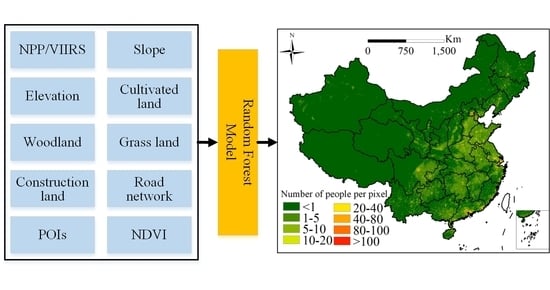
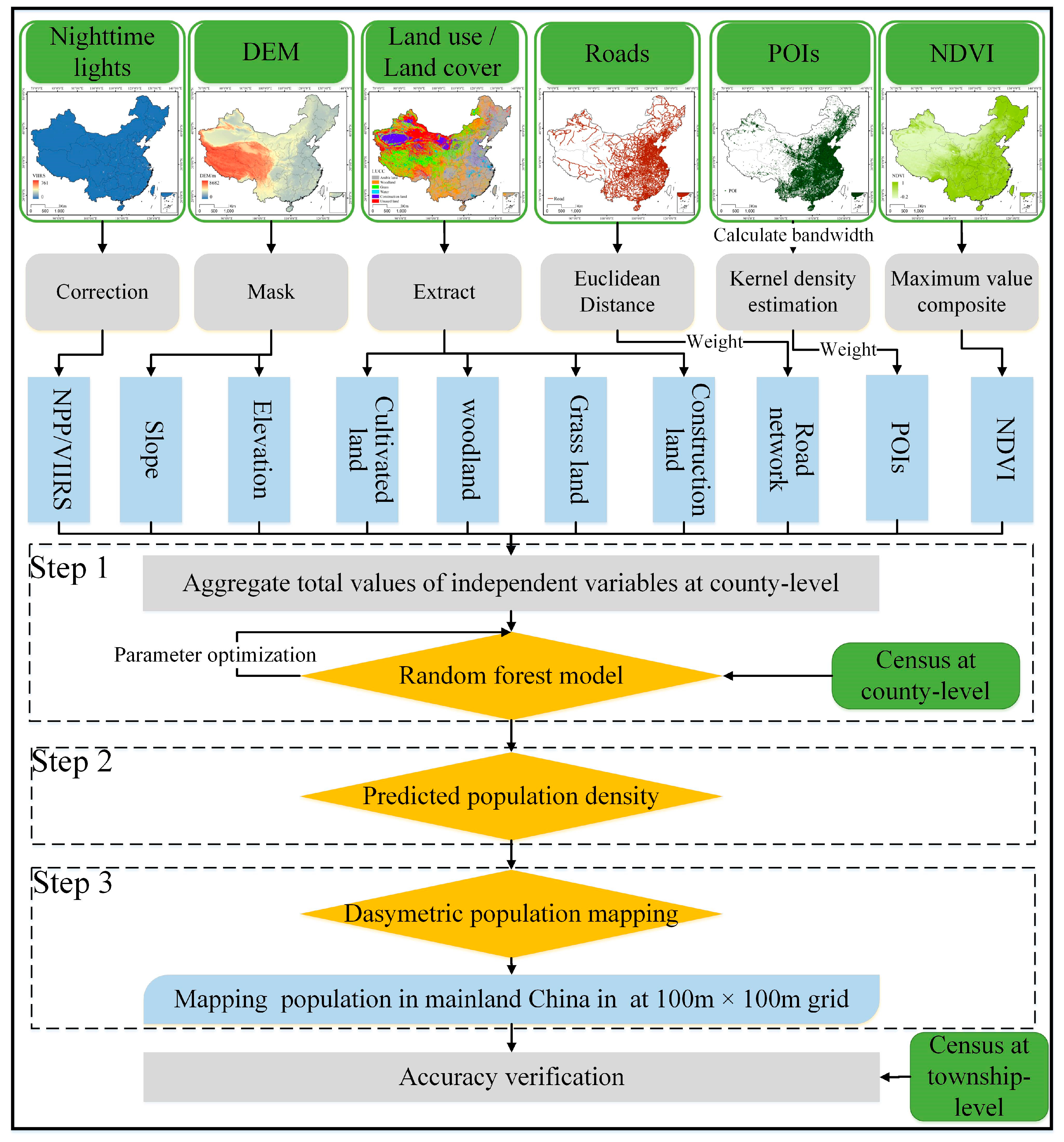
3.1. Mapping the Population Density with the RF Model
3.2. Preprocessing of the Remote Sensing Data and Geographic Big Data
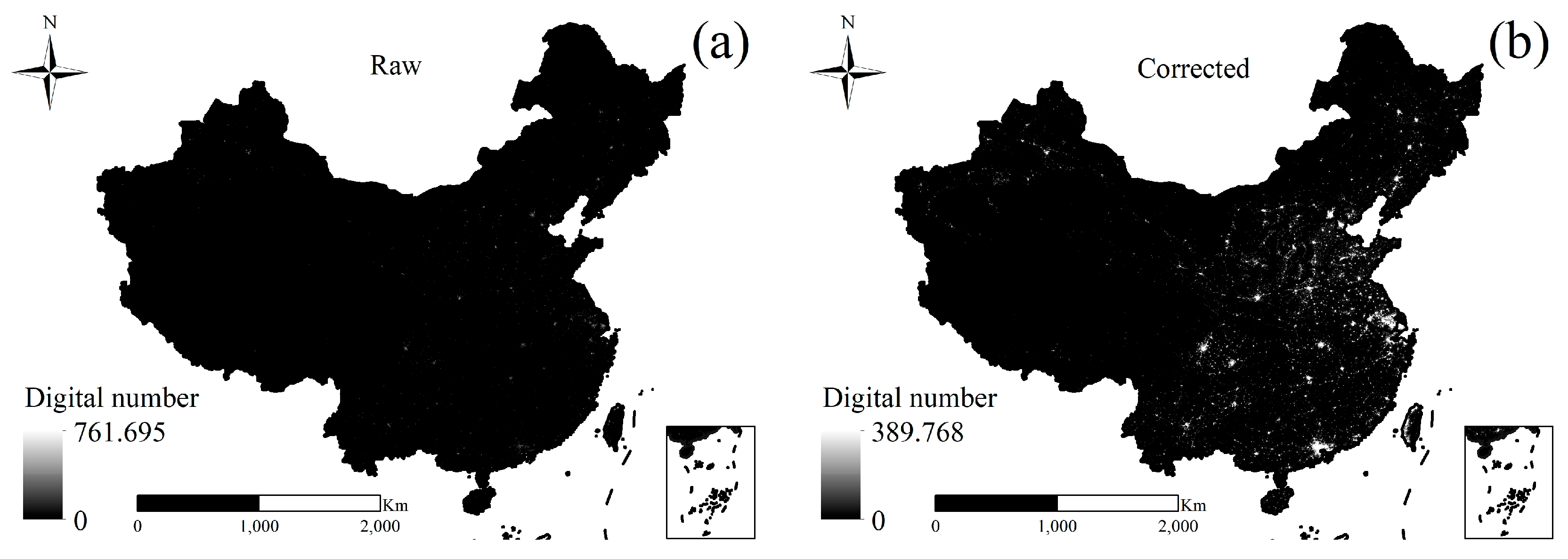
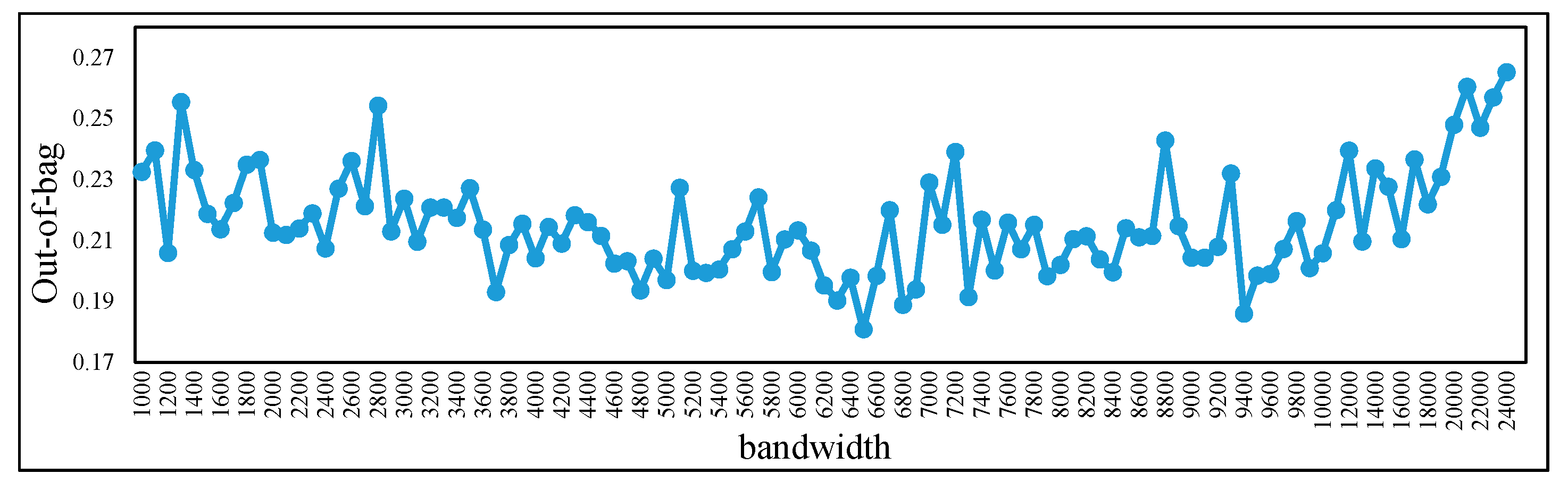
3.2.1. Eliminating the Background Noise and Extreme Values of the NPP/VIIRS Data
3.2.2. Producing NDVI Annual Synthetic Data
3.2.3. Generating the POI Density Layers
3.2.4. Calculating the Road Distance Layers
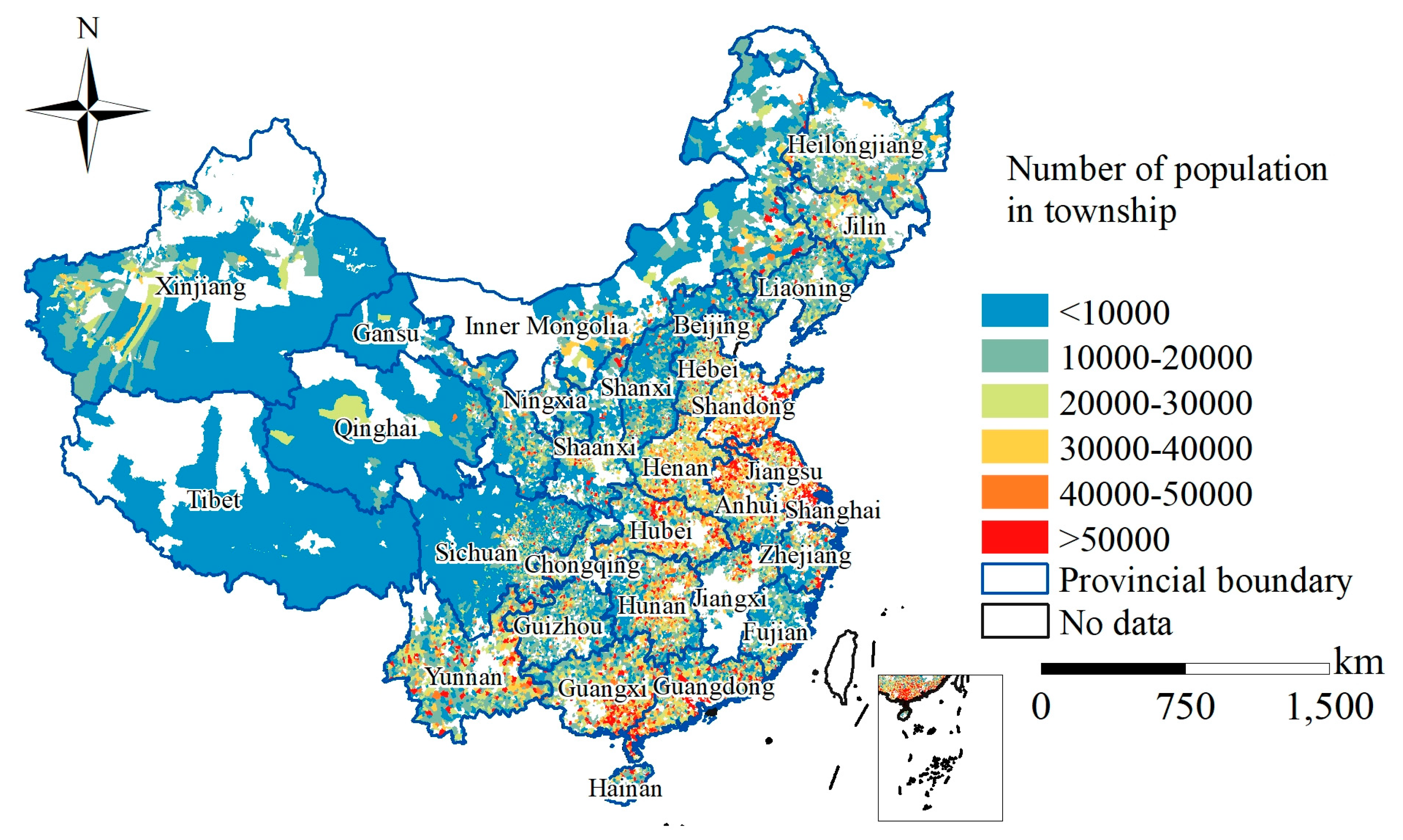
3.3. Accuracy Assessment
4. Results
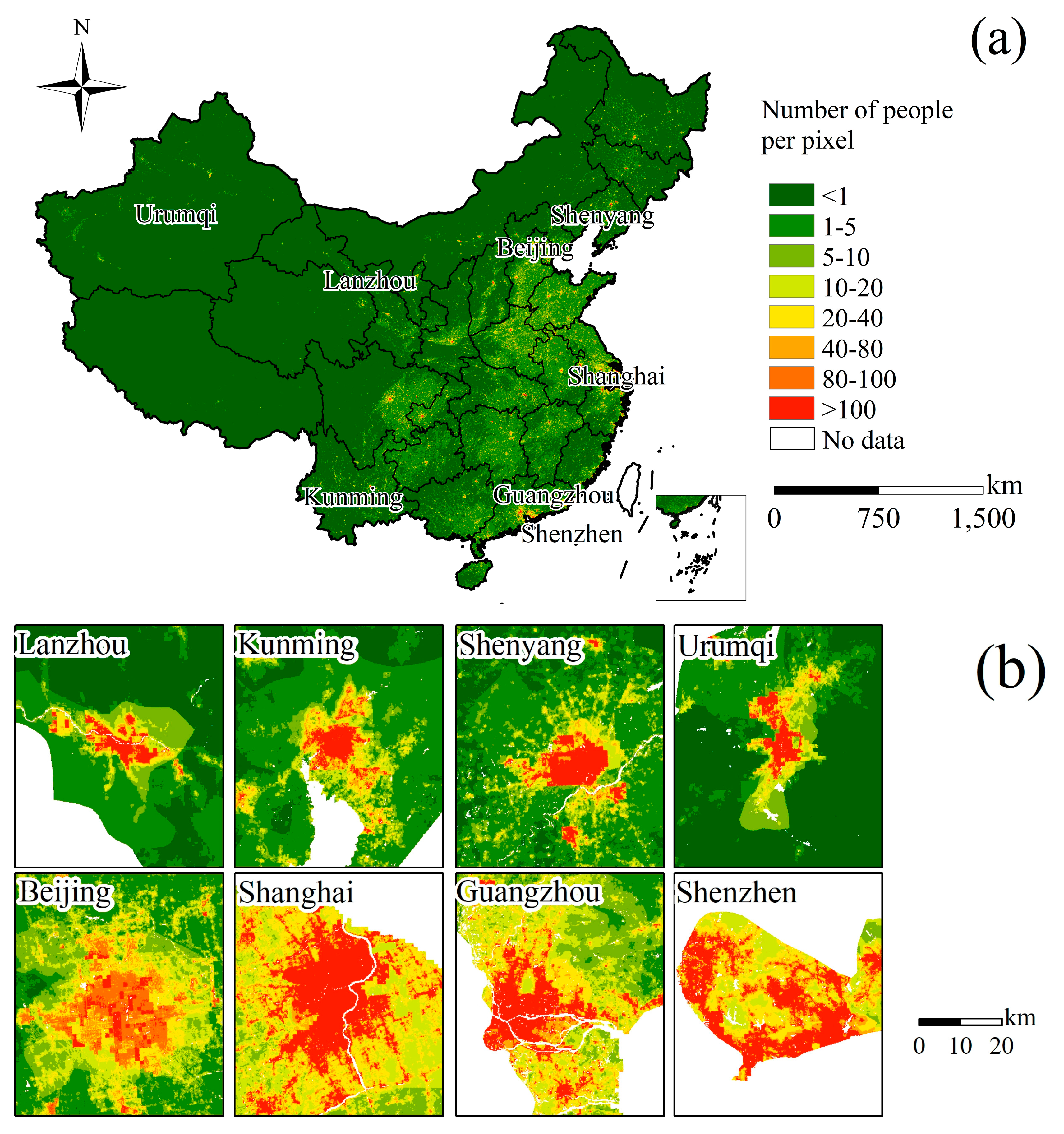
4.1. Results of the Population Density Mapping
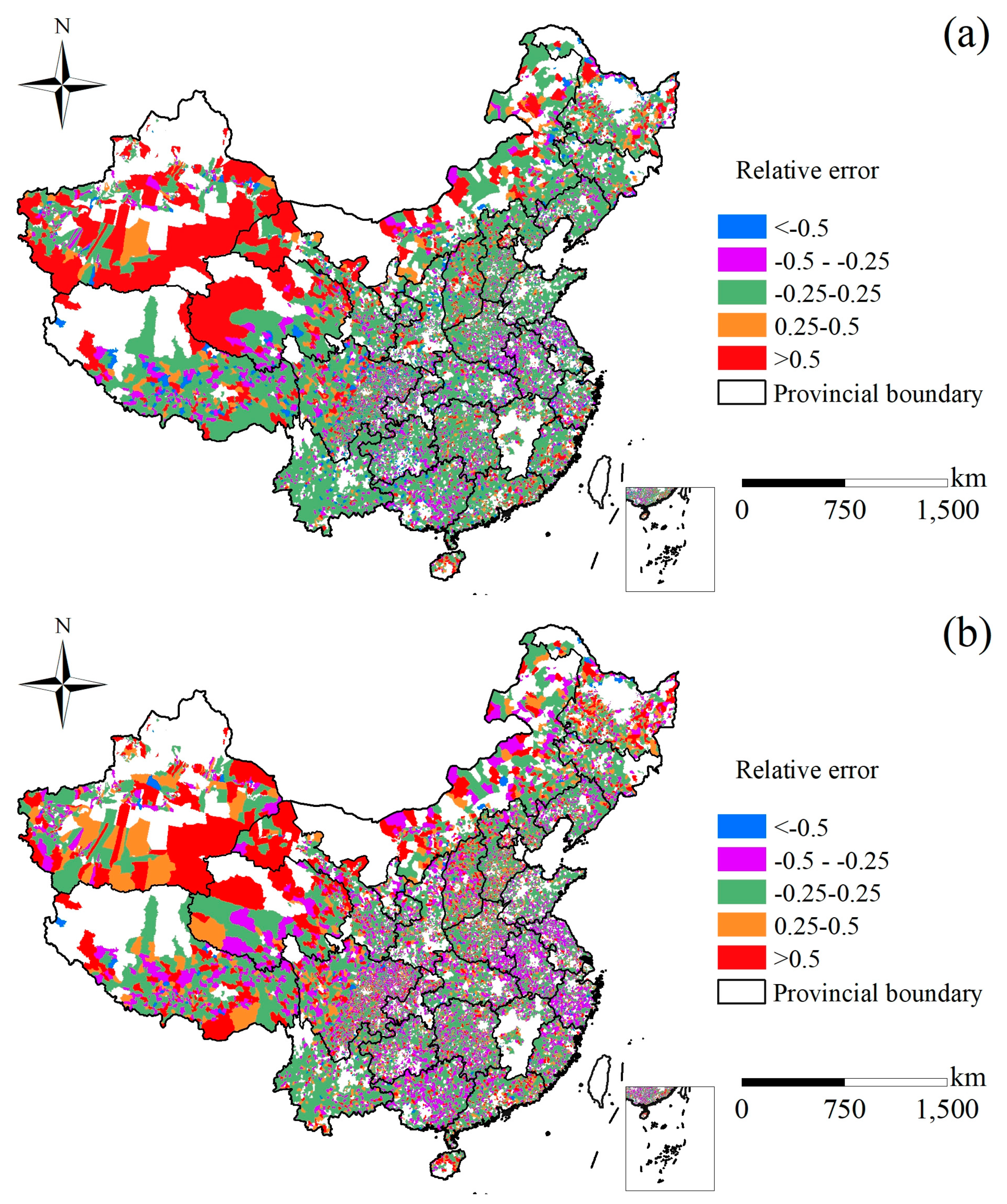
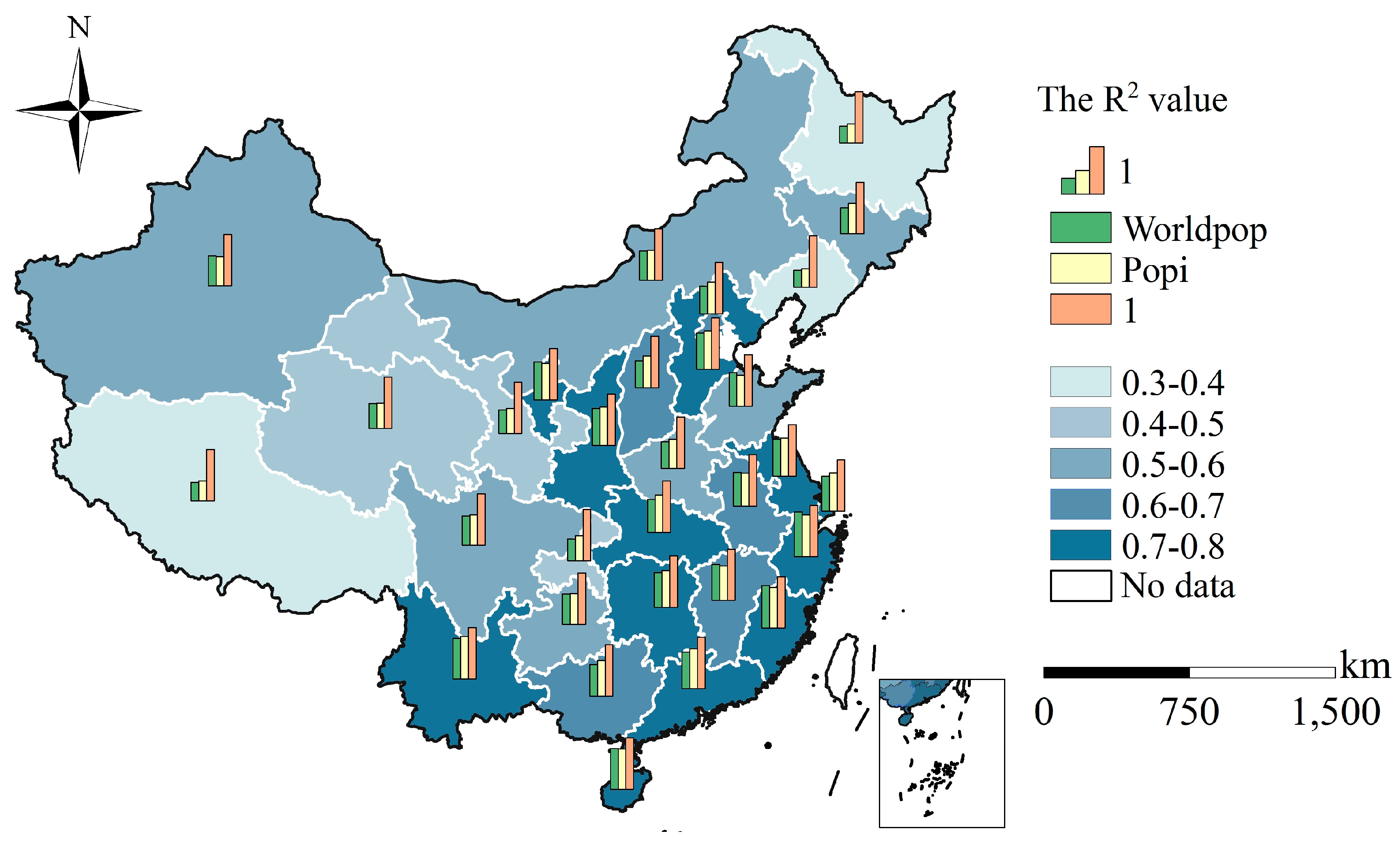
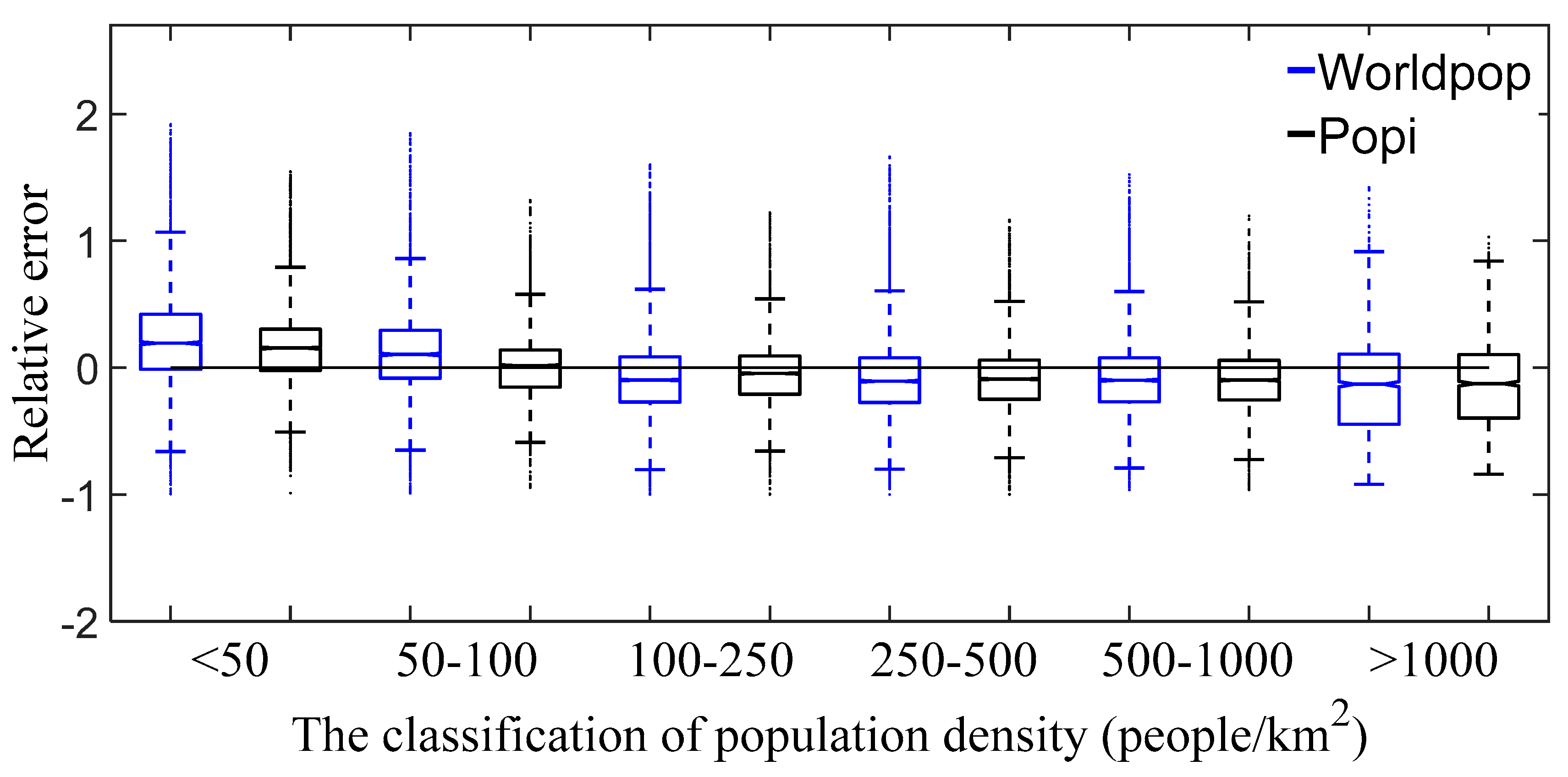
4.2. Accuracy Assessment
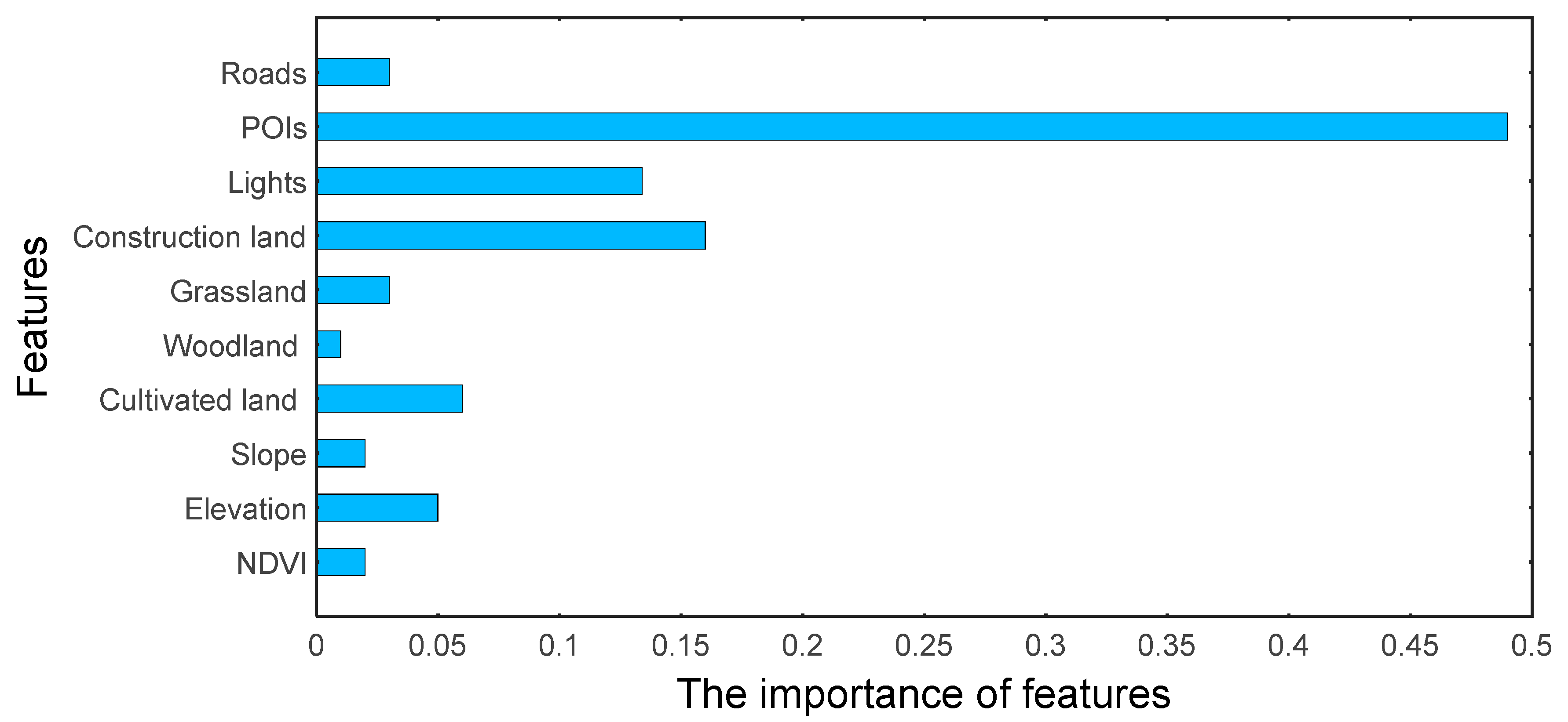
4.3. The Feature Importance of the Independent Variables
5. Discussion
5.1. The Differences between POIs and NPP/VIIRS in Mapping the Population Density
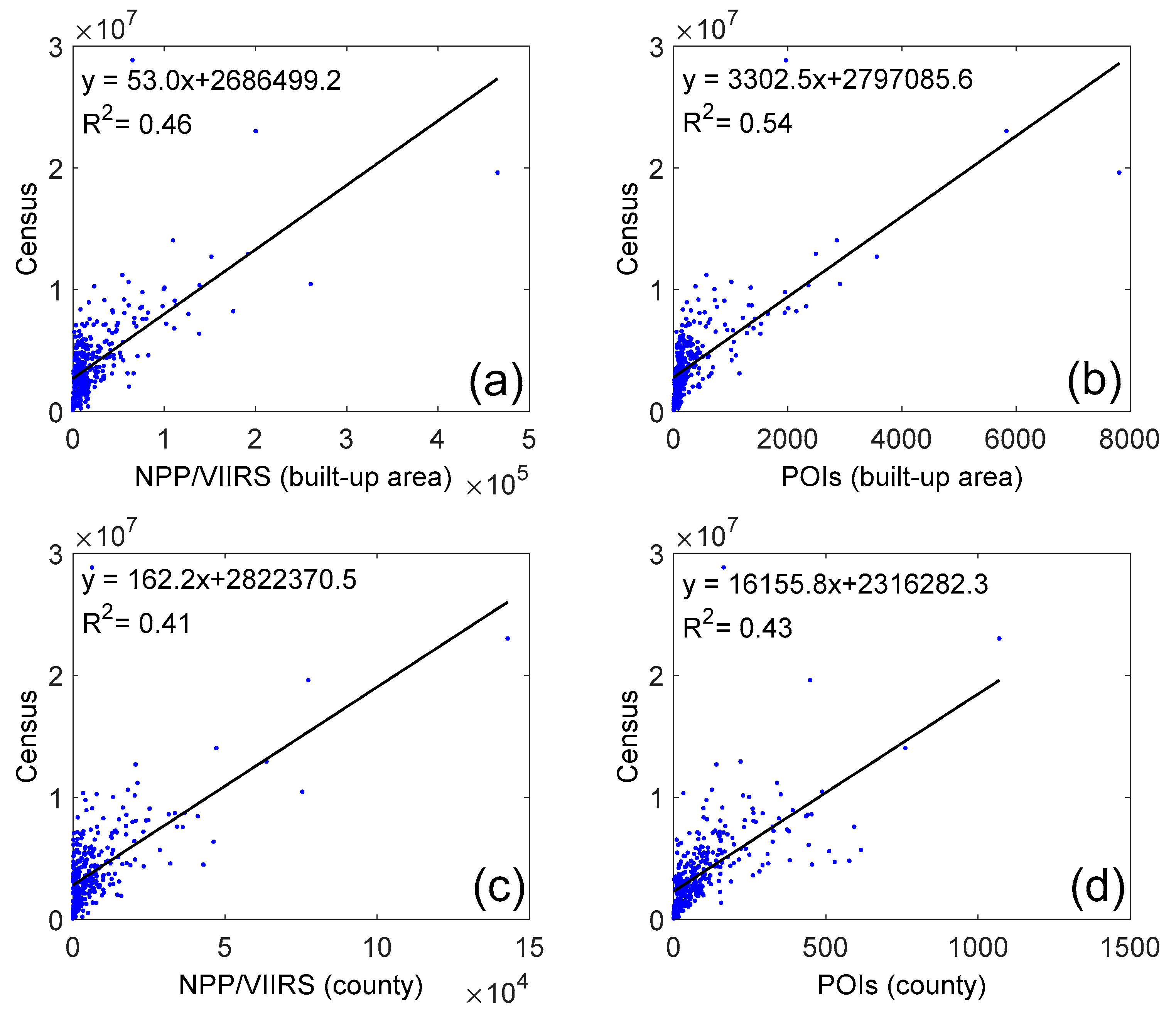
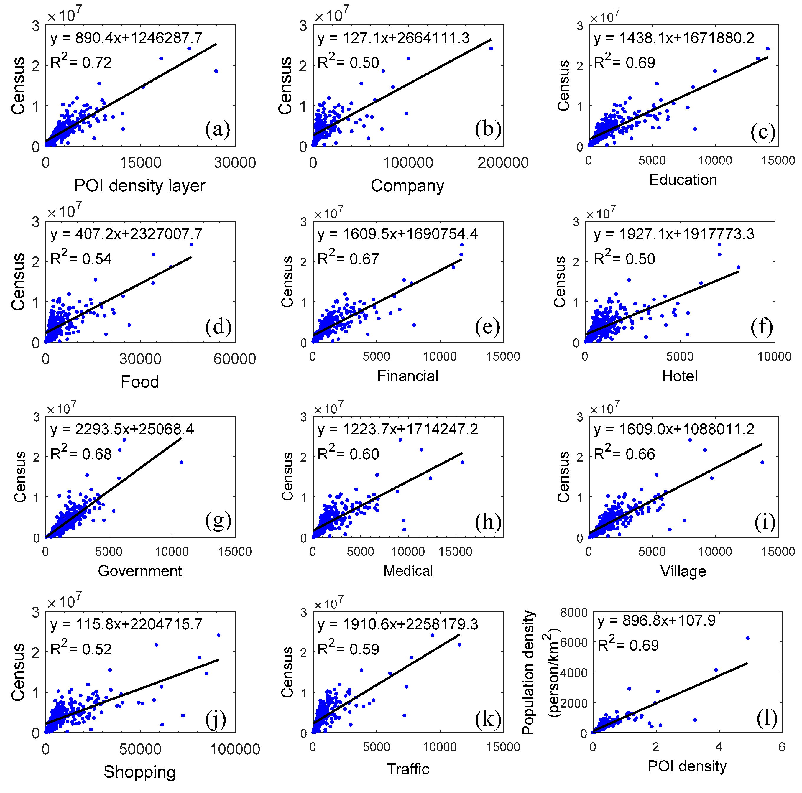
5.2. The Correlation between POIs and Censuses
5.3. Error Analysis
6. Conclusions
Author Contributions
Funding
Acknowledgments
Conflicts of Interest
References
- Lu, D.; Tian, H.; Zhou, G.; Ge, H. Regional mapping of human settlements in southeastern China with multisensor remotely sensed data. Remote Sens. Environ. 2008, 112, 3668–3679. [Google Scholar] [CrossRef]
- Ferguson, N.M.; Cummings, D.A.; Cauchemez, S.; Fraser, C.; Riley, S.; Meeyai, A.; Iamsirithaworn, S.; Burke, D.S. Strategies for containing an emerging influenza pandemic in Southeast Asia. Nature 2005, 437, 209–214. [Google Scholar] [CrossRef] [PubMed] [Green Version]
- Storeygard, A.; Balk, D.; Levy, M.; Deane, G. The Global Distribution of Infant Mortality: A subnational spatial view. Popul. Space Place 2008, 14, 209–229. [Google Scholar] [CrossRef] [Green Version]
- Balk, D.; Storeygard, A.; Levy, M.; Gaskell, J.; Sharma, M.; Flor, R. Child hunger in the developing world: An analysis of environmental and social correlates. Food Policy 2005, 30, 584–611. [Google Scholar] [CrossRef]
- Wang, Y.; Huang, C.; Feng, Y.; Zhao, M.; Gu, J. Using Earth Observation for Monitoring SDG 11.3.1-Ratio of Land Consumption Rate to Population Growth Rate in Mainland China. Remote Sens. 2020, 12, 357. [Google Scholar] [CrossRef] [Green Version]
- Gaughan, A.E.; Stevens, F.R.; Huang, Z.; Nieves, J.J.; Sorichetta, A.; Lai, S.; Ye, X.; Linard, C.; Hornby, G.M.; Hay, S.I.; et al. Spatiotemporal patterns of population in mainland China, 1990 to 2010. Sci. Data 2016, 3, 160005. [Google Scholar] [CrossRef] [PubMed]
- Openshaw, S. A million or so correlation coefficients: Three experiments on the modifiable areal unit problem. In Statistical Applications in the Spatial Sciences; Wrigley, N., Ed.; Pion: London, UK, 1979; pp. 127–144. [Google Scholar]
- Dong, C.; Liu, J.; Zhao, R.; Wang, G. An discussion on correlation of geographical parameter with spatial population distribution. Remote Sens. Inform. 2002, 4, 61–64. [Google Scholar]
- Bai, Z.; Wang, J.; Wang, M.; Gao, M.; Sun, J. Accuracy Assessment of Multi-Source Gridded Population Distribution Datasets in China. Sustainability 2018, 10, 1363. [Google Scholar] [CrossRef] [Green Version]
- Deichmann, U.; Balk, D.; Yetman, G. Transforming Population Data for Interdisciplinary Usages: From Census to Grid. In Population Health Metrics; Center for International Earth Science Information Network: Washington, DC, USA, 2001. [Google Scholar]
- Balk, D.L.; Deichmann, U.; Yetman, G.; Pozzi, F.; Hay, S.I.; Nelson, A. Determining Global Population Distribution: Methods, Applications and Data. In Global Mapping of Infectious Diseases: Methods, Examples and Emerging Applications; Academic Press: London, UK, 2006; pp. 119–156. [Google Scholar]
- Dobson, J.E.; Bright, E.A.; Coleman, P.R.; Durfee, R.C.; Worley, B.A. LandScan: A Global Population Database for Estimating Populations at Risk. Photogramm. Eng. Remote Sens. 2000, 66, 849–857. [Google Scholar]
- Jiang, D.; Yang, X.; Wang, N.; Liu, H. Study on spatial distribution of population based on remote sensing and GIS. Adv. Earth Sci. 2002, 17, 734–738. [Google Scholar]
- Stevens, F.R.; Gaughan, A.E.; Linard, C.; Tatem, A.J. Disaggregating census data for population mapping using random forests with remotely-sensed and ancillary data. PLoS ONE 2015, 10, e0107042. [Google Scholar] [CrossRef] [Green Version]
- Zhuo, L.; Ichinose, T.; Zheng, J.; Chen, J.; Shi, P.J.; Li, X. Modelling the population density of China at the pixel level based on DMSP/OLS non-radiance-calibrated night-time light images. Int. J. Remote Sens. 2009, 30, 1003–1018. [Google Scholar] [CrossRef]
- Hsu, F.; Baugh, K.; Ghosh, T.; Zhizhin, M.; Elvidge, C. DMSP-OLS Radiance Calibrated Nighttime Lights Time Series with Intercalibration. Remote Sens. 2015, 7, 1855–1876. [Google Scholar] [CrossRef] [Green Version]
- Zhao, J.; Ji, G.; Yue, Y.; Lai, Z.; Chen, Y.; Yang, D.; Yang, X.; Wang, Z. Spatio-temporal dynamics of urban residential CO2 emissions and their driving forces in China using the integrated two nighttime light datasets. Appl. Energy 2019, 235, 612–624. [Google Scholar] [CrossRef]
- Wang, X.; Sutton, P.C.; Qi, B. Global Mapping of GDP at 1 km2 Using VIIRS Nighttime Satellite Imagery. ISPRS Int. J. Geo-Inf. 2019, 8, 580. [Google Scholar] [CrossRef] [Green Version]
- Chen, X. Nighttime Lights and Population Migration: Revisiting Classic Demographic Perspectives with an Analysis of Recent European Data. Remote Sens. 2020, 12, 169. [Google Scholar] [CrossRef] [Green Version]
- Elvidge, C.D.; Sutton, P.C.; Ghosh, T.; Tuttle, B.T.; Baugh, K.E.; Bhaduri, B.; Bright, E. A global poverty map derived from satellite data. Comput. Geosci. 2009, 35, 1652–1660. [Google Scholar] [CrossRef]
- Yu, B.; Lian, T.; Huang, Y.; Yao, S.; Ye, X.; Chen, Z.; Yang, C.; Wu, J. Integration of nighttime light remote sensing images and taxi GPS tracking data for population surface enhancement. Int. J. Geogr. Inf. Sci. 2018, 33, 687–706. [Google Scholar] [CrossRef]
- Gao, S.; Janowicz, K.; Couclelis, H. Extracting urban functional regions from points of interest and human activities on location-based social networks. Trans. GIS 2017, 21, 446–467. [Google Scholar] [CrossRef]
- Bakillah, M.; Liang, S.; Mobasheri, A.; Arsanjani, J.J.; Zipf, A. Fine-resolution population mapping using OpenStreetMap points-of-interest. Int. J. Geogr. Inf. Sci. 2014, 28, 1940–1963. [Google Scholar] [CrossRef]
- Li, K.; Chen, Y.; Li, Y. The Random Forest-Based Method of Fine-Resolution Population Spatialization by Using the International Space Station Nighttime Photography and Social Sensing Data. Remote Sens. 2018, 10, 1650. [Google Scholar] [CrossRef] [Green Version]
- Yao, Y.; Liu, X.; Li, X.; Zhang, J.; Liang, Z.; Mai, K.; Zhang, Y. Mapping fine-scale population distributions at the building level by integrating multisource geospatial big data. Int. J. Geogr. Inf. Sci. 2017, 31, 1220–1244. [Google Scholar] [CrossRef]
- Wang, L.; Fan, H.; Wang, Y. Improving population mapping using Luojia 1-01 nighttime light image and location-based social media data. Sci. Total Environ. 2020, 730, 139–148. [Google Scholar] [CrossRef]
- Sutton, P.C. Modeling population density with night-time satellite imagery and GIS. Comput. Environ. Urban Syst. 1997, 21, 227–244. [Google Scholar] [CrossRef]
- Wang, L.; Wang, S.; Zhou, Y.; Liu, W.; Hou, Y.; Zhu, J.; Wang, F. Mapping population density in China between 1990 and 2010 using remote sensing. Remote Sens. Environ. 2018, 210, 269–281. [Google Scholar] [CrossRef]
- Wang, L.; Fan, H.; Wang, Y. Fine-Resolution Population Mapping from International Space Station Nighttime Photography and Multisource Social Sensing Data Based on Similarity Matching. Remote Sens. 2019, 11, 1900. [Google Scholar] [CrossRef] [Green Version]
- Breiman, L. Random forests. Mach. Learn. 2001, 45, 5–32. [Google Scholar] [CrossRef] [Green Version]
- Liu, J.; Kuang, W.; Zhang, Z.; Xu, X.; Qin, Y.; Ning, J.; Zhou, W.; Zhang, S.; Li, R.; Yan, C.; et al. Spatiotemporal characteristics, patterns, and causes of land-use changes in China since the late 1980s. J. Geogr. Sci. 2014, 24, 195–210. [Google Scholar] [CrossRef]
- Liu, J.; Liu, M.; Tian, H.; Zhuang, D.; Zhang, Z.; Zhang, W.; Tang, X.; Deng, X. Spatial and temporal patterns of China’s cropland during 1990–2000: An analysis based on Landsat TM data. Remote Sens. Environ. 2005, 98, 442–456. [Google Scholar] [CrossRef]
- Shi, K.; Yu, B.; Huang, Y.; Hu, Y.; Yin, B.; Chen, Z.; Chen, L.; Wu, J. Evaluating the Ability of NPP-VIIRS Nighttime Light Data to Estimate the Gross Domestic Product and the Electric Power Consumption of China at Multiple Scales: A Comparison with DMSP-OLS Data. Remote Sens. 2014, 6, 1705–1724. [Google Scholar] [CrossRef] [Green Version]
- Sun, M.; Wang, T.; Xu, X.; Zhang, L.; Li, J.; Shi, Y. Ecological risk assessment of soil cadmium in China’s coastal economic development zone: A meta-analysis. Ecosyst. Health Sustain. 2020, 6, 1733921. [Google Scholar] [CrossRef] [Green Version]
- Li, X.; Levin, N.; Xie, J.; Li, D. Monitoring hourly night-time light by an unmanned aerial vehicle and its implications to satellite remote sensing. Remote Sens. Environ. 2020, 247, 111942. [Google Scholar] [CrossRef]
- Dobler, G.; Ghandehari, M.; Koonin, S.E.; Nazari, R.; Patrinos, A.; Sharma, M.S.; Tafvizi, A.; Vo, H.T.; Wurtele, J.S. Dynamics of the urban lightscape. Inform. Syst. 2015, 54, 115–126. [Google Scholar] [CrossRef] [Green Version]
- Yang, X.; Ye, T.; Zhao, N.; Chen, Q.; Yue, W.; Qi, J.; Zeng, B.; Jia, P. Population Mapping with Multisensor Remote Sensing Images and Point-Of-Interest Data. Remote Sens. 2019, 11, 574. [Google Scholar] [CrossRef] [Green Version]
- Chun, J.; Zhang, X.; Huang, J.; Zhang, P. A Gridding Method of Redistributing Population Based on POIs. Geogr. Geo-Inf. Sci. 2018, 34, 83–89. (In Chinese) [Google Scholar]
- Lloyd, C.T.; Sorichetta, A.; Tatem, A.J. High resolution global gridded data for use in population studies. Sci. Data 2017, 4, 170001. [Google Scholar] [CrossRef] [PubMed] [Green Version]
- Zhao Xin, S.Y.; Liu, Y.; Chen, F.; Hu, Y. Population Spatialization Based on Satellite Remote Sensing and POI Data: Guangzhou as an Example. Trop. Geogr. 2020, 40, 101–109. [Google Scholar]
- Patel, N.N.; Stevens, F.R.; Huang, Z.; Gaughan, A.E.; Elyazar, I.; Tatem, A.J. Improving Large Area Population Mapping Using Geotweet Densities. Trans. GIS 2016, 21, 317–331. [Google Scholar] [CrossRef]
- Li, X.; Ma, R.; Zhang, Q.; Li, D.; Liu, S.; He, T.; Zhao, L. Anisotropic characteristic of artificial light at night—Systematic investigation with VIIRS DNB multi-temporal observations. Remote Sens. Environ. 2019, 233, 111357. [Google Scholar] [CrossRef]
- Tian, Y.; Zhou, Q.; Fu, X. An Analysis of the Evolution, Completeness and Spatial Patterns of OpenStreetMap Building Data in China. ISPRS Int. J. Geo-Inf. 2019, 8, 35. [Google Scholar] [CrossRef] [Green Version]
- Liu, Y.; Zhu, A.X.; Wang, J.; Li, W.; Hu, G.; Hu, Y. Land-use decision support in brownfield redevelopment for urban renewal based on crowdsourced data and a presence-and-background learning (PBL) method. Land Use Policy 2019, 88, 104188. [Google Scholar] [CrossRef]
- Jiang, Y.; Li, Z.; Ye, X. Understanding demographic and socioeconomic biases of geotagged Twitter users at the county level. Cartogr. Geogr. Inf. Sci. 2018, 46, 228–242. [Google Scholar] [CrossRef]


| Datasets | Data Declaration | Time | Sources |
|---|---|---|---|
| NPP/VIIRS | 750 m | 2015 | National Oceanic and Atmospheric Administration, (NOAA) (https://ngdc.noaa.gov/eog/viirs/download_dnb_composites.html) |
| POIs | Point features | 2015 | Baidu Maps API (http://lbsyun.baidu.com/) |
| Land use/ land cover | 100 m | 2015 | Chinese Academy of Sciences Resource and Environmental Science Data Center (http://www.resdc.cn/data.aspx?DATAID=99) |
| NDVI | 250 m | 2015 | Moderate-resolution Imaging Spectroradiometer (MODIS) (http://ladsweb.modaps.eosdis.nasa.gov/) |
| DEM | 90 m | 2000 | National Aeronautics and Space Administration (NASA) (http://srtm.csi.cgiar.org/srtmdata/) |
| Roads | Line features | 2015 | Baidu Maps Application Programming Interface (API) (http://lbsyun.baidu.com/) |
| Census | County Township | 2015 | 2016 Statistical Yearbook of Provinces and Cities, National Bureau of Statistics of China (http://www.stats.gov.cn/tjsj/pcsj/, http://www.ngcc.cn/ngcc/) |
| Worldpop | 100 m | 2015 | University of Southampton (https://www.worldpop.org/geodata/listing?id=16) |
| Administrative boundary map | County Township | 2015 | National Fundamental Geography Information System (http://www.ngcc.cn/ngcc/) |
| Classification | Content |
|---|---|
| Transportation | Airports, railway stations, bus stations, terminals, ferries, etc. |
| Government | Government agencies |
| Village | Villages |
| Education | Universities, research institutes, middle schools, kindergartens, etc. |
| Food | Restaurants, canteens, etc. |
| Medical | Hospitals, pharmacies, health service stations, clinics, etc. |
| Entertainment | Business centers, supermarkets, shops, wholesale markets, etc. |
| Accommodation | Guest, hotels, etc. |
| Working place | Companies, factories, etc. |
| Financial | ATMs, banks, savings centers, etc. |
| Categories | Transportation | Government | Village | Education | Food |
| Weight | 0.096 | 0.103 | 0.105 | 0.106 | 0.094 |
| Categories | Medical | Entertainment | Accommodation | Working Place | Financial |
| Weight | 0.104 | 0.098 | 0.099 | 0.092 | 0.105 |
| Categories | Railway | National Road | Provincial Road | Highway |
| Weight | 0.140 | 0.151 | 0.138 | 0.139 |
| Categories | Urban Road | County Road | Village Road | |
| Weight | 0.161 | 0.128 | 0.143 |
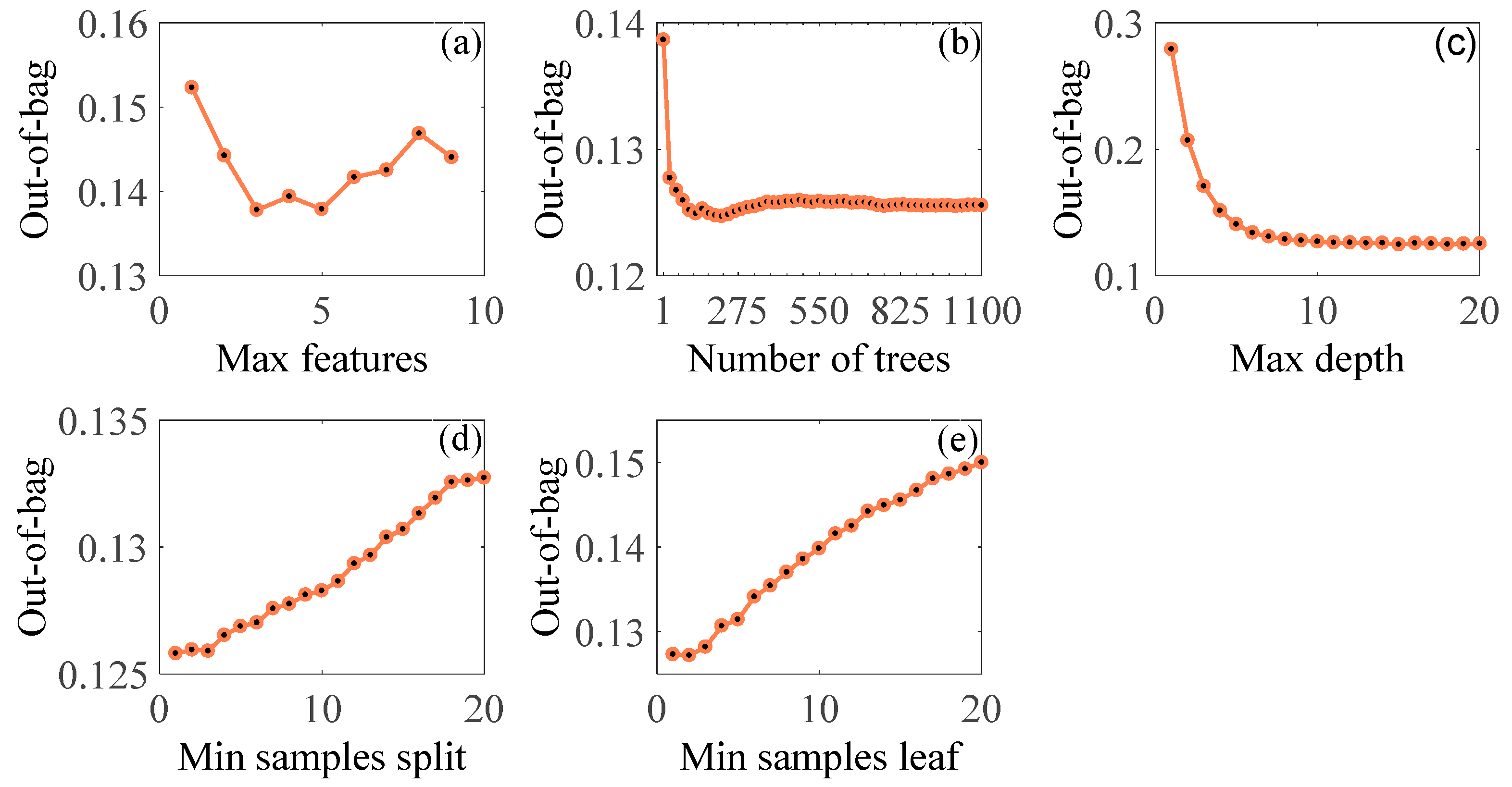
| Parameter Type | Range | Optimal Value |
|---|---|---|
| Max. features | 1–10 | 5 |
| Number of trees | 1–1100 | 200 |
| Max. depth | 1–20 | 15 |
| Min. samples split | 2–20 | 2 |
| Min. samples leaf | 1–20 | 1 |
Publisher’s Note: MDPI stays neutral with regard to jurisdictional claims in published maps and institutional affiliations. |
© 2020 by the authors. Licensee MDPI, Basel, Switzerland. This article is an open access article distributed under the terms and conditions of the Creative Commons Attribution (CC BY) license (http://creativecommons.org/licenses/by/4.0/).
Share and Cite
Wang, Y.; Huang, C.; Zhao, M.; Hou, J.; Zhang, Y.; Gu, J. Mapping the Population Density in Mainland China Using NPP/VIIRS and Points-Of-Interest Data Based on a Random Forests Model. Remote Sens. 2020, 12, 3645. https://0-doi-org.brum.beds.ac.uk/10.3390/rs12213645
Wang Y, Huang C, Zhao M, Hou J, Zhang Y, Gu J. Mapping the Population Density in Mainland China Using NPP/VIIRS and Points-Of-Interest Data Based on a Random Forests Model. Remote Sensing. 2020; 12(21):3645. https://0-doi-org.brum.beds.ac.uk/10.3390/rs12213645
Chicago/Turabian StyleWang, Yunchen, Chunlin Huang, Minyan Zhao, Jinliang Hou, Ying Zhang, and Juan Gu. 2020. "Mapping the Population Density in Mainland China Using NPP/VIIRS and Points-Of-Interest Data Based on a Random Forests Model" Remote Sensing 12, no. 21: 3645. https://0-doi-org.brum.beds.ac.uk/10.3390/rs12213645