A More Reliable Orbit Initialization Method for LEO Precise Orbit Determination Using GNSS

School of Geodesy and Geomatics, Wuhan University, 430079 Wuhan, China
*
Author to whom correspondence should be addressed.
Remote Sens. 2020, 12(21), 3646; https://0-doi-org.brum.beds.ac.uk/10.3390/rs12213646
Submission received: 16 October 2020
/
Revised: 4 November 2020
/
Accepted: 5 November 2020
/
Published: 6 November 2020
(This article belongs to the Special Issue Advances in GNSS Data Processing and Navigation)
Abstract
:Precise orbit determination (POD) using GNSS has been rapidly developed and is the mainstream technology for the navigation of low Earth orbit (LEO) satellites. The initialization of orbit parameters is a key prerequisite for LEO POD processing. For a LEO satellite equipped with a GNSS receiver, sufficient discrete kinematic positions can be obtained easily by processing space-borne GNSS data, and its orbit parameters can thus be estimated directly in iterative manner. This method of direct iterative estimation is called as the direct approach, which is generally considered highly reliable, but in practical applications it has risk of failure. Stability analyses demonstrate that the direct approach is sensitive to oversized errors in the starting velocity vector at the reference time, which may lead to large errors in design matrix because the reference orbit may be significantly distorted, and eventually cause the divergence of the orbit parameter estimation. In view of this, a more reliable method, termed the progressive approach, is presented in this paper. Instead of estimating the orbit parameters directly, it first fits the discrete kinematic positions to a reference ephemeris in the form of the GNSS broadcast ephemeris, which construct a reference orbit that is smooth and close to the true orbit. Based on the reference orbit, the starting orbit parameters are computed in sufficient accuracy, and then the final orbit parameters are estimated with a high accuracy by using discrete kinematic positions as measurements. The stability analyses show that the design matrix errors are reduced in the progressive approach, which would assure more robust orbit parameter estimation than the direct estimation approach. Various orbit initialization experiments are performed on the KOMPSAT-5 and FY3C satellites. The results have fully verified the high reliability of the proposed progressive approach.
1. Introduction
With the great progress of Global Navigation Satellite System (GNSS), high-precision orbit determination using space-borne GNSS data has been the most mainstream technology for the navigation of low Earth orbit (LEO) satellites, due to its global coverage, abundant observations and low-cost [1,2]. Only with a GNSS receiver onboard LEO satellites, a lot of continuous GNSS measurements are generated without time and geography limitation. By processing the space-borne GNSS data, precise orbits at centimeter level can be achievable, hence the technique of precise orbit determination (POD) using GNSS has been applied to a wide range of LEO satellites nowadays [3,4,5]. In the dynamical orbit determination, the orbit parameters, including the position and velocity at the reference time and several piece-wise dynamical coefficients, such as the atmospheric drag coefficient, the solar radiation pressure coefficient and empirical acceleration coefficients, should be initialized first by fitting the discrete positions, before being accurately estimated [6]. This process, which is called “orbit initialization”, is a key prerequisite for the successful operation of LEO POD. The successful implementation of orbit initialization is rarely suspected because sufficient discrete positions are available for orbit parameters estimation when they are generated by Standard Point Positioning (SPP) or Precise Point Positioning (PPP) using abundant GNSS measurements [7]. Therefore, various researches about orbit initialization always concentrated on space debris only with rare short-arc range, angle or angle-rate data [8,9,10,11,12], instead of the LEO satellites using GNSS. In recent years, LEO constellations of hundreds of satellites for positioning, navigation, timing, remote sensing and communication (PNTRC) services have gradually become an emerging trend in the field of satellite navigation [13,14,15]. Thousands of LEO satellites are or will be deployed in the future and stable precise orbits are necessary for PNTRC services, so the reliable orbit initialization becomes more and more important, especially for the automated POD or integrated POD processing of many LEO satellites [14,15]. However, the orbit initialization still faces the risk of unreliability, even if the abundant GNSS measurements are available, due to complex orbit dynamics and different GNSS data quality.
Based on the discrete kinematic positions generated by Standard Point Positioning (SPP) or Precise Point Positioning (PPP) using GNSS data, the position and velocity at the reference time and all piece-wise dynamical coefficients of LEO satellites can be estimated together directly by a least squares estimator and the estimation process is usually iterative until the estimator converges. This method is called here “the direct approach”. The estimation process of the direct approach is simple and convenient and the orbit initial parameters could be obtained easily after several iterations of estimation. This approach is usually the default orbit initialization approach for LEO POD using GNSS. However, in the direct approach, the iterative estimation of orbit parameters requires a starting state first, and its accuracy has an unignorable effect on the estimation convergence. If the starting values for some orbit parameters, especially the velocity at the reference time, are not accurate enough, the numerically integrated orbit and state transition matrix would have errors growing with time from the reference epoch and accumulated to large values. These accumulated errors may lead to the inaccurate orbit estimation, or even cause the divergence of the iterative estimation. More generally, the starting position and velocity at the reference time are computed by the interpolation of discrete kinematic positions or using GNSS pseudo-range and Doppler observations directly [16]. For the piece-wise dynamical coefficients, their starting values are always set to zero or nominal ones. Although the staring position error at the reference time can be limited to the range of several centimeters to several meters if the GNSS pseudo-range and carrier-phase measurements are processed with simple outlier detection in SPP/PPP, it is very difficult to absolutely select an epoch with sufficiently small velocity error as the reference time due to the higher sensitivity of integrated orbit and state transition matrix to the velocity. Hence, the direct approach has a risk to cause the divergence of orbit parameter estimation.
It must be pointed out that, for a single LEO satellite, this type of estimation divergence may occur rarely, and if it happens, the divergent orbit can be discarded directly. However, in the automated POD processing of thousands of LEO satellites, removing the divergent arcs directly would decrease partly not only the availability of LEO precise orbits but also the effective utilization of space-borne GNSS data. In addition, for the automated integrated POD processing of GNSS/LEO satellites, multiple LEO satellites or even the LEO constellation are treated as the special tracking stations to enhance the geometry of the GNSS POD, which is able to overcome limited geometrical strength from ground tracking network only and improve the POD accuracy of GNSS/LEO satellites simultaneously [14,15]. In this scenario, removing the divergent arcs of some LEO satellites means that, not only can’t the precise orbits of these satellites be generated, but also the enhanced capacity of the LEO tracking network on GNSS orbit determination may decrease. What is more serious, the orbit parameters of LEO and GNSS are all estimated together in the integrated POD, so the orbit parameters from different LEO satellites are related closely. Therefore, if a divergence occurs on one satellite and if it is not discovered and removed in time, it will affect the orbit estimation of GNSS satellites, and then interfere with other LEO satellites inevitably, and even cause the collapse of the overall integrated POD process. Consequently, a more reliable orbit initialization method is important to avoid such fatal error and guarantee stable POD processing.
This paper proposes a more reliable orbit initialization method to improve the stability of the precise LEO orbit estimation. The new method first constructs a reference orbit for a LEO satellite by estimating a set of orbit parameters in the form of the GNSS broadcast ephemeris based on the SPP/PPP discrete kinematic positions. For the convenience, this set of orbit parameters is referred as the LEO reference ephemeris. Then, the LEO reference ephemeris can be used to generate a series of tabular positions and velocities. Although the LEO reference ephemeris can’t describe the orbit accurately and the errors of generated tabular positions may be of hundreds or thousands of meters, the resultant reference orbit is nevertheless smooth and close to the true orbit, such that the precise orbit parameters can be estimated stably with the starting position and velocity vectors at the reference epoch of guaranteed accuracy. In a step-by-step approach, the estimated orbit parameters in the previous step are used to compute the starting orbit state for the next direct estimation, and accurate orbit parameters are estimated directly by taking the SPP/PPP discrete kinematic positions as observations for the POD. In a summary, the orbit parameters are obtained by adopting a step-wise manner in the new method, so it is called “the progressive approach”.
In the following section, the direct approach will be briefly introduced first. Then, the progressive approach is presented in detail. Next, the corresponding methods and tests will be designed to have an in-depth understanding on the estimation stability of these two approaches. After that, these two approaches will be applied to the orbit initialization experiments of real LEO missions such as KOMPSAT-5 and FY3C. Some cases will be compared and discussed in detail to validate the high stability of the progressive approach. Finally, some conclusions are made.
2. Orbit Initialization Methods
2.1. The Direct Approach
The equation of the motion of a LEO satellite can be expressed as:
where ( are the position, velocity and acceleration vectors of the satellite in a geocentric inertial coordinate frame, respectively, and p represents the dynamical coefficients in the force models, including the atmospheric drag coefficient Cd and the solar radiation pressure coefficient Cr. To account for those un-modeled forces that act on the LEO satellite or for the inaccurate force models, the empirical accelerations w = (aR,aA,aC) in the radial (R), along-track (A) and cross (C) directions are customarily introduced in the POD processing, where some empirical parameters, including the one-cycle-per-revolution coefficients in the R/A/C directions, are estimated [17]. These to-be-estimated empirical parameters are also treated as a part of the vector p. f(·) is a function expression that represents the acceleration , and is related to the position, velocity and dynamical coefficients of the satellite. According to Equation (1), the first-order differential equation of the motion of the satellite is formed:
A dynamical orbit can be expressed by a set of orbit parameters in the form of the position r0 and velocity at a reference time t0 and the dynamical coefficients p. In order to express the orbit more precisely, the dynamical coefficients p are always set to be piece-wise constant (PWC), thus they are called PWC parameters. All to-be-estimated orbit parameters are abbreviated as a vector: . According to differential Equation (2), the position r at any epoch t can be expressed by an implicit function:
where, it is difficult to compute the explicit formulation of g(·) because of the high non-linearity of differential Equation (2). However, it is obvious that, using a series of discrete kinematic positions (r(t1), r(t2),…, r(tn)) at the subsequent epochs (t1,t2,…,tn) as measurements, the orbit parameters X can be estimated.
In the estimation process, setting the starting state of the orbit parameters X = X* first, observation Equation (3) can be linearized as:
where, dX* is the estimated correction vector to the starting state X*. r*(t) = g(X*,t) is the computed position based on the starting state X*. is the state transition matrix, which represents the first-order partial derivative of the position with respect to the estimated orbit parameters. o(X*,dX*,t) is the remainder of linearization, which is relative to the starting state X* and the correction vector dX*. Although g(·) cannot be expressed by an explicit formulation, r*(t) and can be computed by the numerical integration of differential Equation (2) [18]. dX* is the unknown parameter to be estimated, so the remainder o(X*,dX*,t) is unknown and cannot be computed. It should be neglected in order to estimate dX* by the least squares method.
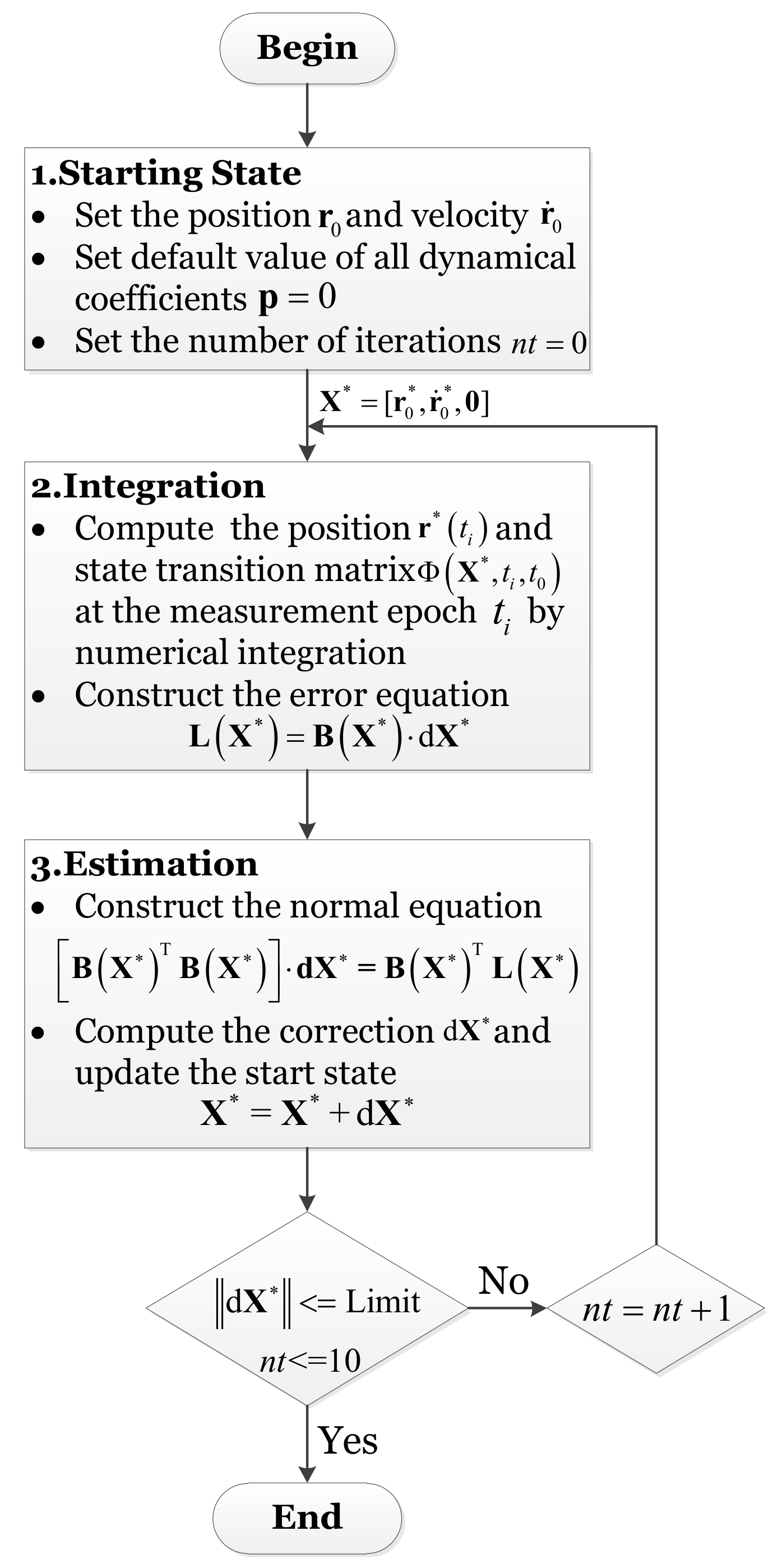
According to Equation (4), the orbit parameters are estimated iteratively, and the iterative estimation process of the direct approach is designed as Figure 1. The processing scheme mainly consists of three steps. First, the starting state of the orbit parameters is initialized as X*, where the position r0 and velocity at the reference time t0 are valued directly by the interpolation of the SPP/PPP discrete kinematic positions, and other dynamical coefficients are always set as 0.0 or their nominal values such as 2.2 for the drag coefficient. Then, based on the starting state X*, the predicted positions r*(t) and state transition matrix within the whole estimated arc are computed by the numerical integration of the motion equations. The positions r*(ti) and state transition matrix at each measurement epoch (t1,t2,…,tn) can be computed by an interpolation method. Thus, error Equation (4) can be constructed. Finally, the normal equation is obtained, and the correction dX* is estimated by the least squares method. Generally, the second and third steps should be performed iteratively, until the convergence condition is satisfied. Obviously, the oversized errors in the starting state X* may cause the divergence of the iterative estimation of orbit parameters.
2.2. The Progressive Approach
The progressive approach doesn’t estimate the orbit parameters directly, but it first fits the discrete kinematic positions to a reference ephemeris Y, which has the same parameters in the GNSS broadcast ephemeris [19]:
where, A is the semi-major axis, i0, M0 and Ω0 are the orbital inclination, mean anomaly and right ascension of the ascending node at the reference time t0, respectively, e is the eccentricity, and w is the argument of perigee. Δn represents the difference between the average and computed angular velocity. and are the rates of orbital inclination and the right ascension of the ascending node, respectively. Cuc and Cus are the amplitudes of the cosine and sine correction terms to the latitude angle, respectively. Crc and Crs are those to the orbital radius, and Cic and Cis to the orbital inclination. The first six parameters are the Keplerian orbit elements, which can be computed directly by from the position and velocity vectors. The following three parameters are the supplements to the main Keplerian orbit elements. The last six parameters (Cuc, Cus, Crc, Crs, Cic, Cis) are to account for the perturbation effects on the latitude angle, radius and inclination.
Using the SPP/PPP discrete kinematic positions as measurements, the parameters in the reference ephemeris can be estimated. The starting state of the six main Keplerian orbit elements are computed from the position and velocity at the reference time t0, and other parameters are set as 0.0. Regarding the starting state of the reference ephemeris Y* as the nominal state, observation Equation (3) can be linearized as:
where, dY* is the estimated correction to the starting state Y*. r*(t) is the position computed from the starting state Y*. φ(Y*,t,t0) is the state transition matrix, which represents the first-order partial derivative of the position with respect to the reference ephemeris. Both r*(t) and φ(Y*,t,t0) can be computed by using an explicit analytical formula [20]. υ(Y*,dY*,t) is the remainder of linearization. Similarly, the unknown remainder υ(Y*,dY*,t) should be neglected in order to estimate dY* by the least squares method.
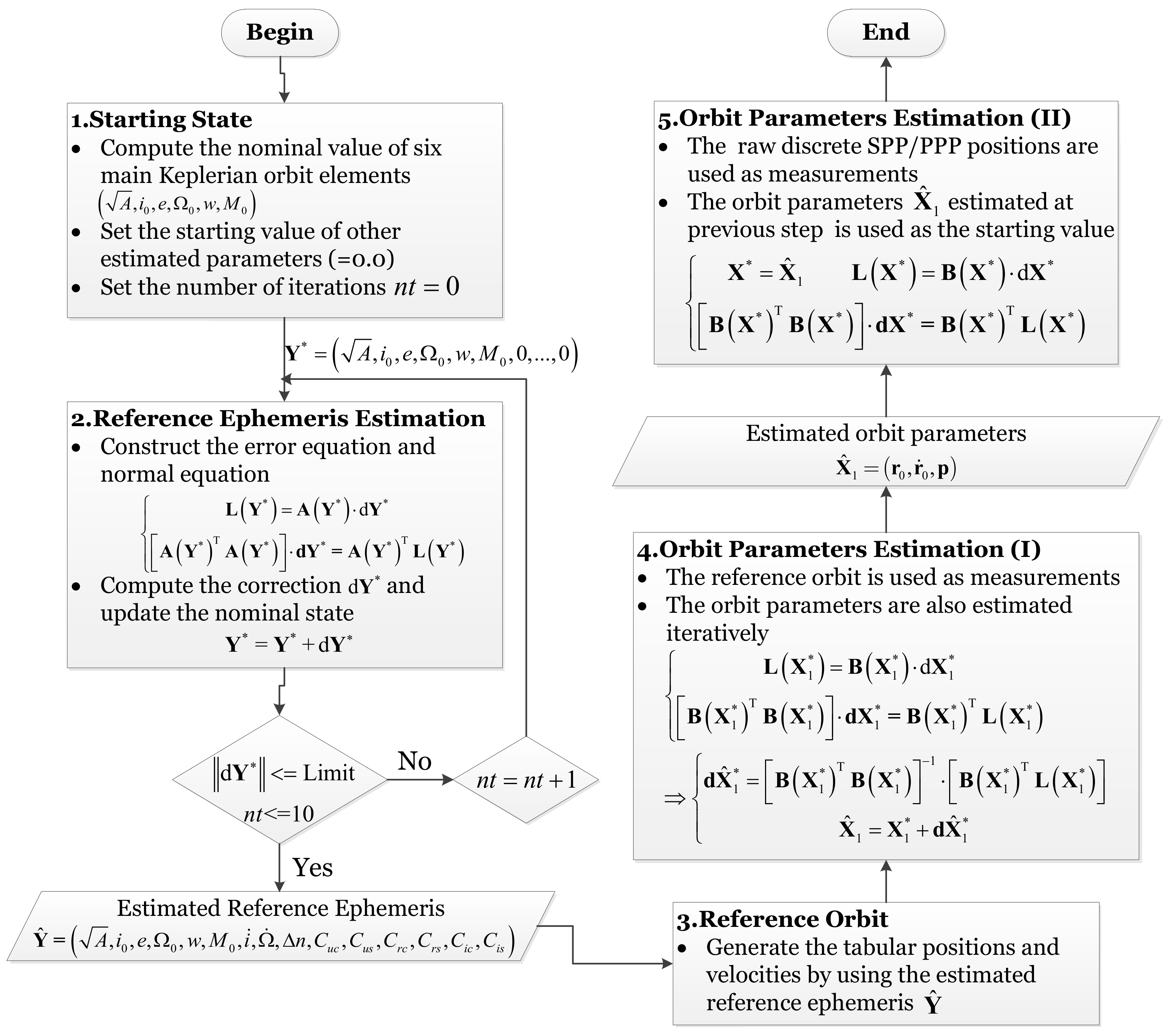
The estimation processing scheme of the progressive approach is shown in Figure 2. The processing scheme mainly consists of five steps. First, the starting state of Keplerian orbit elements is computed from the position and velocity vectors at an arbitrary epoch. Next, the parameters in the reference ephemeris are estimated iteratively by using only the SPP/PPP discrete kinematic positions as measurements. This generates a reference orbit. Although the position errors of the reference orbit may be at the level of hundreds or even thousands of meters, the determined reference orbit is smooth and continuous, and close to the true orbit. Then, the orbit parameters are estimated by using the tabular positions of reference orbit as measurements. Unlike the SPP/PPP discrete kinematic positions, the reference orbit is smooth and follows the orbit dynamics. So it can provide a starting position and velocity with enough accuracy to estimate a set of orbit parameters reliably that coincide with the tabular positions of reference orbit. Finally, the estimated orbit parameters are used as the starting state, and the raw SPP/PPP discrete kinematic positions are used as measurements, to determine the final orbit parameters iteratively. Because the starting state of the orbit parameters , which represents the reference orbit, is close to the true orbit, the errors in the starting state would have negligible impact on the iterative estimation of final orbit parameters.
3. Stability Analyses
3.1. Effect of the Starting State Error
According to Figure 1, the iterative estimation of orbit parameters in the direct approach is at the risk of divergence if the errors in the starting state X* are too large. In the linear Equation (4), X* appears in three terms: (1) L(X*), (2) B(X*) and (3) o(X*,dX*). L(X*) is the difference between the observed and computed positions, which is used as measurements to estimate the correction d X*. B(X*) is the design matrix, and o(X*,dX*) is the linearization remainder which should be small enough to neglect. If X* has large errors, the neglect of remainder o(X,dX*) and errors in B(X*) will severely distort error Equation (5), which may lead to a divergence of the iterative estimation. The neglected remainder o(X*,dX*) can be treated as the linearization error, and the errors in the design matrix B(X*) is called as the design error, which are both originated from the errors of the starting value X*. If the start value X* is not equal to the true value, the linearization error cannot be avoided, but the iterative estimation can reduce the linearization error, assuming that there is no error of the design matrix B(X*) or the design error is controlled well. Therefore, the design error is essential to the success of iterative estimation. Setting the true value of the orbit parameters as Tx and the true design matrix as M, the error of the starting value X* is dX* = Tx − X*, and the error of the design matrix B(X*) is M − B(X*). It is difficult to express the effect of the design error if using M − B(X*). The expression is more meaningful to describe the design error in the form of:
Here, ERRB is a 3-dimensional vector that expresses the influence of the design matrix B(X*) on the position. The larger ERRB is, the more probably the divergence of iterative estimation occurs. According to Equation (7), the error of starting value dX* decides the design error. If dX* is small enough, ERRB is also not enough to affect the iterative estimation. If dX* is large, ERRB will probably be too large to impact the success of the orbit parameter estimation.
According to Figure 2, the stability of the progressive approach depends on the estimation of parameters in the reference ephemeris. Only when the reference orbit in the form of the reference ephemeris is generated accurately, can the orbit parameters converging to true values be estimated. The generation of the reference orbit is also a process of iterative estimation. Similarly, setting the true parameters in the reference ephemeris as Kx, and the true design matrix as D, the error of the starting value Y* is dY* = Kx − Y*, and the design error can be formed as:
3.2. Stability Analysis Tests
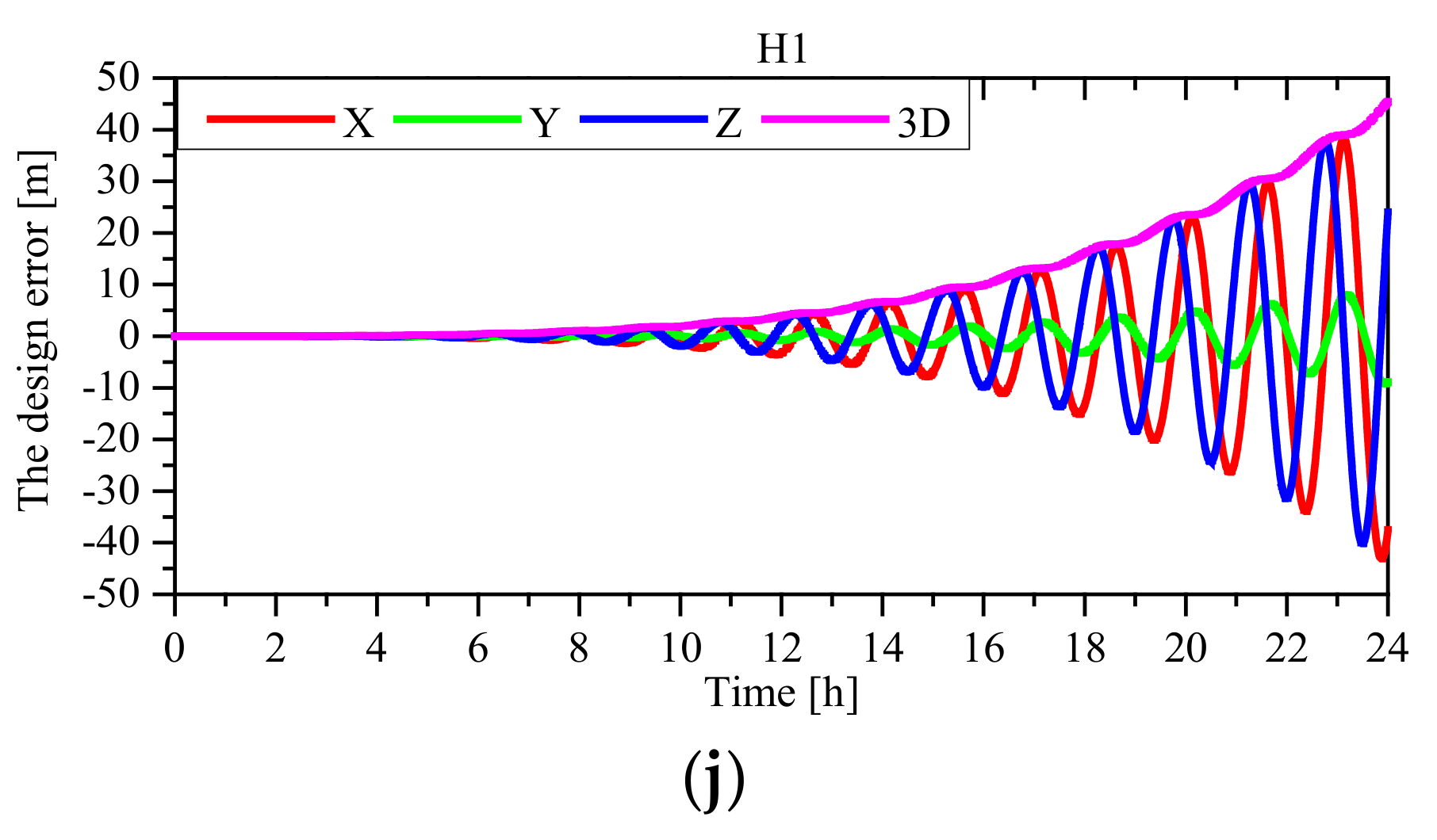
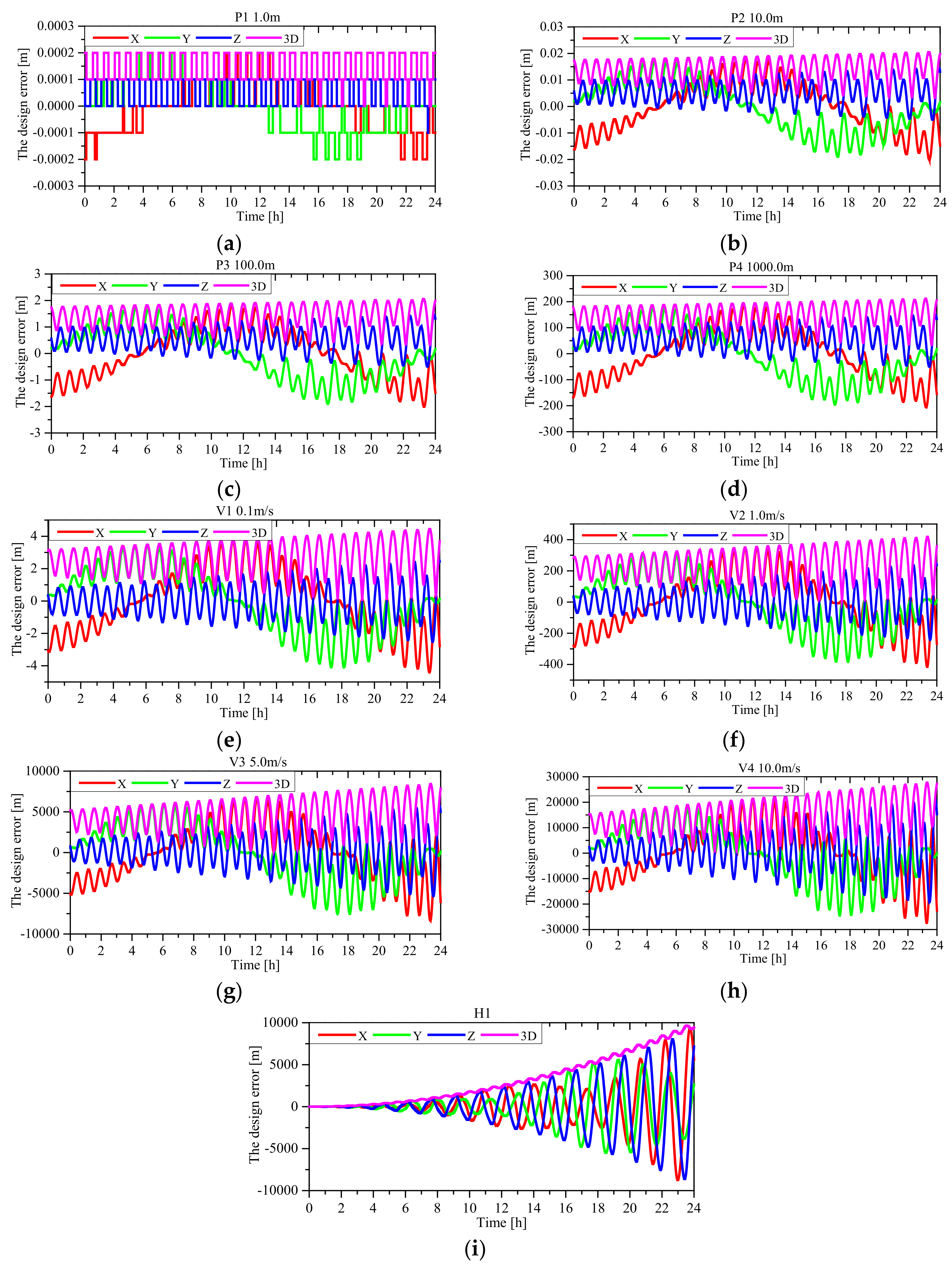
The starting state error dX* consists of three parts: the starting position error dr*, the starting velocity error and the starting dynamical coefficients error dp*. In order to analyze the stability of two orbit initialization methods, the effects of errors in the starting position, velocity and dynamical coefficients are assessed separately. Taking the CHAMP satellite as an example, the starting position and velocity errors of 1.0 m, 10.0 m, 100.0 m, 1000.0 m, 0.1 m/s, 1.0 m/s, 5.0 m/s and 10.0 m/s are set in the X/Y/Z directions at the reference time, respectively, which are abbreviated as P1, P2, P3, P4, V1, V2, V3 and V4, respectively, for convenience. The starting dynamical coefficients are set to 0.0, so their errors are simply the negative of their true values, which are abbreviated as H1. In addition, the length of the whole POD arc is 24 h.
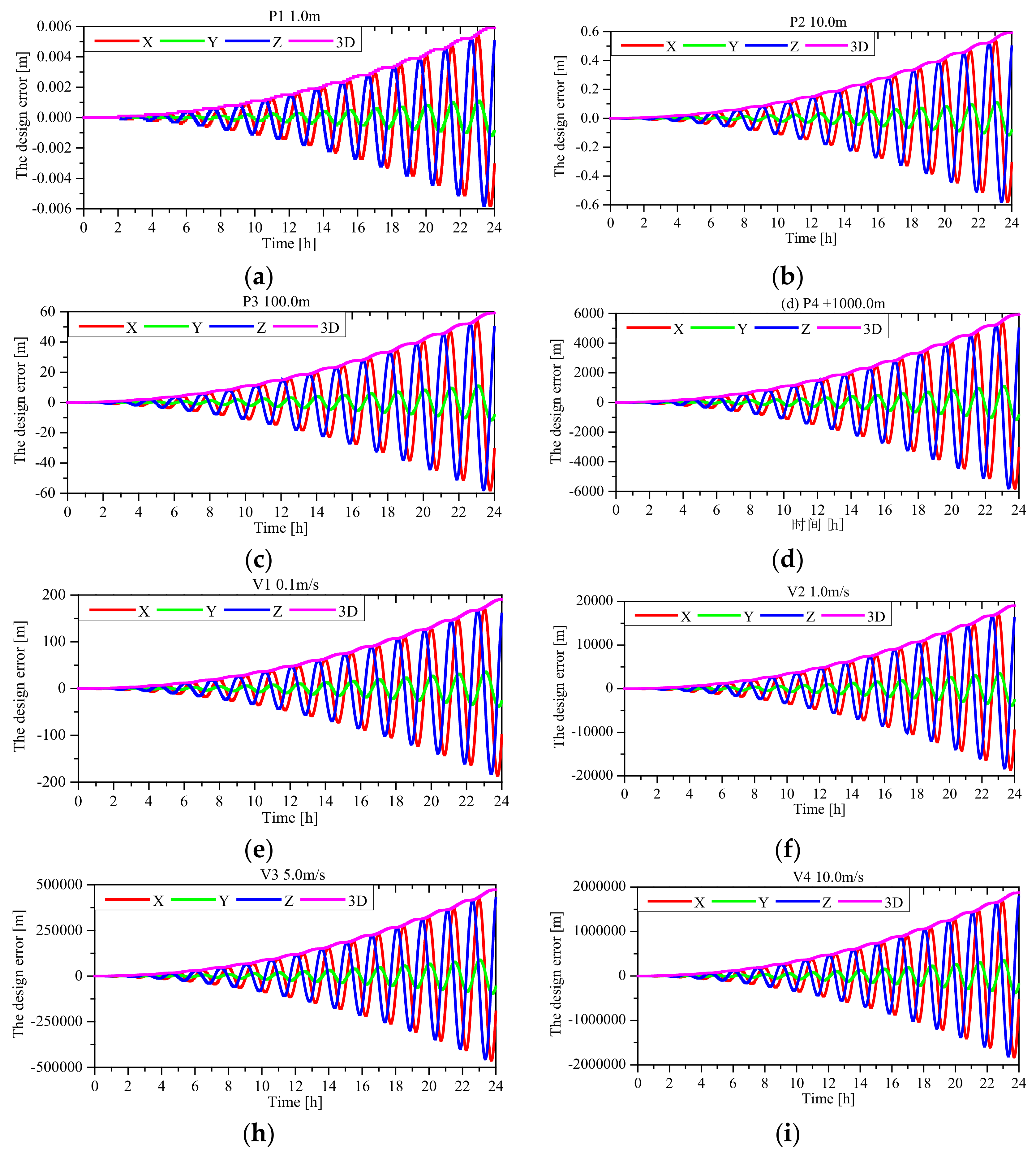
The design errors over 24 h of the direct approach in the X/Y/Z directions and the 3-dimenional (3D) error for the nine cases (P1/P2/P3/V1/V2/V3/V4/H1) are shown in Figure 3. As can be observed clearly, if the orbit parameters are estimated, starting position errors of 1.0, 10.0, 100.0 and 1000.0 m will result in the maximum design errors of about ±0.006, ±0.6, ±60.0, and ±6000.0 m, respectively, while the starting velocity errors of 0.1, 1.0, 5.0 and 10.0 m/s will lead to the maximum design errors of ±200, ±20,000, ±500,000, and ±2,000,000, respectively. The figures show that the design error increases by approximately proportion to the squares of the starting position and velocity error, and it accumulates rapidly as the orbit integration moves forward. In addition, the design error caused by the starting dynamical coefficient error is relatively small, which is only within the range of ±50.0 m. According to the patterns in Figure 3, the design error could reach tens or hundreds of kilometers level if the start position error is up to several or tens of kilometers, while it can soar up to the equivalent level just with the starting velocity error at sub- or several m/s level. Obviously, the design error is more sensitive to the starting velocity error. The main reason for the higher sensitivity to velocity error is that, not only could the velocity error itself produce design errors, but also it can cause the position error accumulated over time away from the reference epoch. Although a rigorous mathematical equation is difficult to derive, an approximate correlation between the starting velocity error at the reference epoch and the position error at an epoch Δt away from the reference epoch may be given as Δp = Δν · Δt to express the influence of the starting velocity on the position error, where Δν is the starting velocity error, Δp represents the position error. Assuming that the starting velocity error is 0.5, the position error will increase up to 43.2 km approximately after 24 h of orbit integration (= 86,000.0 s).
For the LEO satellites at the altitude of hundreds of kilometers, the design error of tens or hundreds of kilometers is likely to cause the divergence of orbit parameter estimation, as a matter of experimental experiences, because it may make the estimated orbit deviate severely from the true orbit. Nevertheless, the staring position error of kilometer level at the reference time can be avoided easily as long as the GNSS pseudo-range and carrier-phase measurements are processed with a simple outlier detection scheme in SPP/PPP, but unfortunately, it is very difficult to prevent the starting velocity error of sub- or several m/s at the reference time absolutely. On the one hand, the position errors of SPP discrete kinematic results are usually at meter level, so the velocity error is easily to reach sub- or several m/s if the velocity is computed by the interpolation of kinematic positions. On the other hand, although the discrete position accuracy of PPP results is always expected at centimeter or decimeter level [6], and the Doppler measurements also can be used for high-precision velocity determination, it is still difficult to preclude the velocity error of sub- or several m/s occurring at certain epochs completely. It is because that, if only a few GNSS satellites are tracked with poor geometric strength, or only less accurate Doppler measurements are available for some LEO satellites at some arcs, the velocity error at certain epochs may still be up to sub- or several m/s [21]. Because it is critical to have an accurately enough starting velocity at the reference epoch for the subsequent POD, one should avoid choosing a reference epoch at which the velocity error happens to be large. However, there would be no external precise orbits as reference to make such choice, the more reliable progressive approach is proposed in this paper to make sure the determined velocity at the reference epoch have sufficient accuracy. Therefore, the orbit parameter estimation is at the risk of having oversized starting velocity error, no matter SPP or PPP discrete kinematic results are used as measurements. It also can be concluded that the oversized starting velocity error is the main possible factor causing the divergence of orbit parameter estimation.
Similarly, the design errors in the X/Y/Z direction and the 3D total error for the nine cases (P1/P2/P3/P4/V1/V2/V3/V4/H1) in reference ephemeris estimation are shown in Figure 4. It should be noted that, in cases of starting position and velocity errors, the position or velocity errors will be transformed to the starting errors of the six Keplerian orbit elements, and H1 represents the errors of other nine parameters in the reference ephemeris. The starting values of the nine parameters are always set as 0.0, so their starting errors are exactly the negative of the true values. As can be observed clearly, the starting position errors of 1.0, 10.0, 100.0 and 1000.0 m result in the design errors at the range of ±0.0003, ±0.03, ±3.0 and ±300.0 m, respectively, and the starting velocity errors of 0.1, 1.0, 5.0 and 10.0 m/s lead to the design errors of ±5.0, ±500, ±10,000 and ±30,000 m. At the same time, the starting errors of the nine parameters cause the design error of ±10,000 m. In addition, the design error doesn’t accumulate rapidly as the orbit integration moves forward far way from the reference time, except for the H1 case.
In the least squares estimator, if the design error of the error equation is too large, the normal equation may become singular, which would result in the divergence of parameter estimation. All in all, the smaller the design error, the more stable the parameter estimation. Comparing Figure 4 with Figure 3, it is obvious that the design errors in the reference ephemeris estimation caused by the same starting position and velocity errors P1/P2/P3/P4/V1/V2/V3/V4 are far less than those in the orbit parameter estimation. Even if the starting velocity error is 10 m/s, the corresponding design error in the reference ephemeris estimation is still less than ±30 km, which is far less than that of ±2000 km in the orbit parameter estimation. It demonstrates that the starting state error has less negative effect on reference ephemeris estimation than on orbit parameter estimation. Although the design error in the reference ephemeris estimation in the case H1 is more than that in orbit parameter estimation, it is still less than ±10 km, which is small enough to perform stable reference ephemeris estimation. Furthermore, the design error in the reference ephemeris estimation would not grow gradually with the orbital integration time. Therefore, it can be concluded that the progressive approach is more stable and reliable than the direct approach to the orbit initialization when there is an oversized starting velocity error.
4. Experiments and Analysis
4.1. Orbit Initialization Experiements
The orbit initialization experiments for comparison of the two approaches will be performed on processing the real-data of KOMPSAT-5 and FY3C satellites. KOMPSAT-5 is the first satellite in Korea that provides 1 m resolution synthetic aperture radar (SAR) images [22]. FY3C is a Chinese meteorological satellite equipped with space-borne GPS/BDS receiver [23]. For the KOMPSAT-5 satellite, the space-borne GPS data is used to compute the discrete kinematic positions by SPP, and the SPP results are used for orbit initialization. For the FY3C satellite, the SPP results based on the space-borne GPS/BDS data are used to estimate initial orbit parameters.
The daily status of the orbit initialization experiments of KOMPSAT-5 on 2016/42~51 and FY3C on 2013/285~294 are summarized in Table 1, where “DA” and “PA” represent the direct approach and progressive approach, respectively. The sign of “×” indicates that the orbit initialization fails, and the sign of “√” the successes. Obviously, the direct approach fails to complete the orbit initialization on 2016/43, 2016/44, 2016/45, 2016/49 and 2016/50 for the KOMPSAT-5 satellite and on 2013/287 and 2013/288 for the FY3C satellite. By contrast, the progressive approach succeeds on all dates.
4.2. Analysis and Discussion
Detailed analyses and discussions are carried out for these dates where the failure of the orbit initialization occurs. According to Figure 1, if using the direct approach, the orbit parameters are estimated iteratively only at the third step. At each iteration step, the resulting orbit parameters are used to compute the position at any epoch and the corresponding 3D position errors are computed by using the precise orbits. According to Figure 2, if using the progressive approach, the reference ephemeris is estimated iteratively at the second step, and the orbit parameters are estimated iteratively at steps 4 and 5. Likewise, the resulting reference ephemeris or orbit parameters of each iteration process at steps 2, 4 and 5 are all used to generate the position sequence and the 3D position errors are computed, too. The 3D position error statistics (RMS) for KOMPSAT-5 and FY3C on their respective failure dates are all shown in Table 2 for each iteration of these two approaches, as well as the mean starting position and velocity errors in the XYZ directions, where “2.X”, “4.X” and “5.X” represent the X-th iteration at steps 2, 4 and 5, respectively. As can be seen clearly, the starting position errors on these days are all less than 3.0 m, but the velocity errors are up to 1~3 m/s, so the oversized velocity errors have caused the estimation divergence in the direct approach. During the iterative process, the position error in each iteration of the direct approach increases until the orbit parameter estimation diverges, while that in the progressive approach decreases gradually until the final orbit parameters are determined. The table shows the step-by-step fitting of orbit parameters in the progressive approach, and also illustrates its reliability for the orbit initialization.
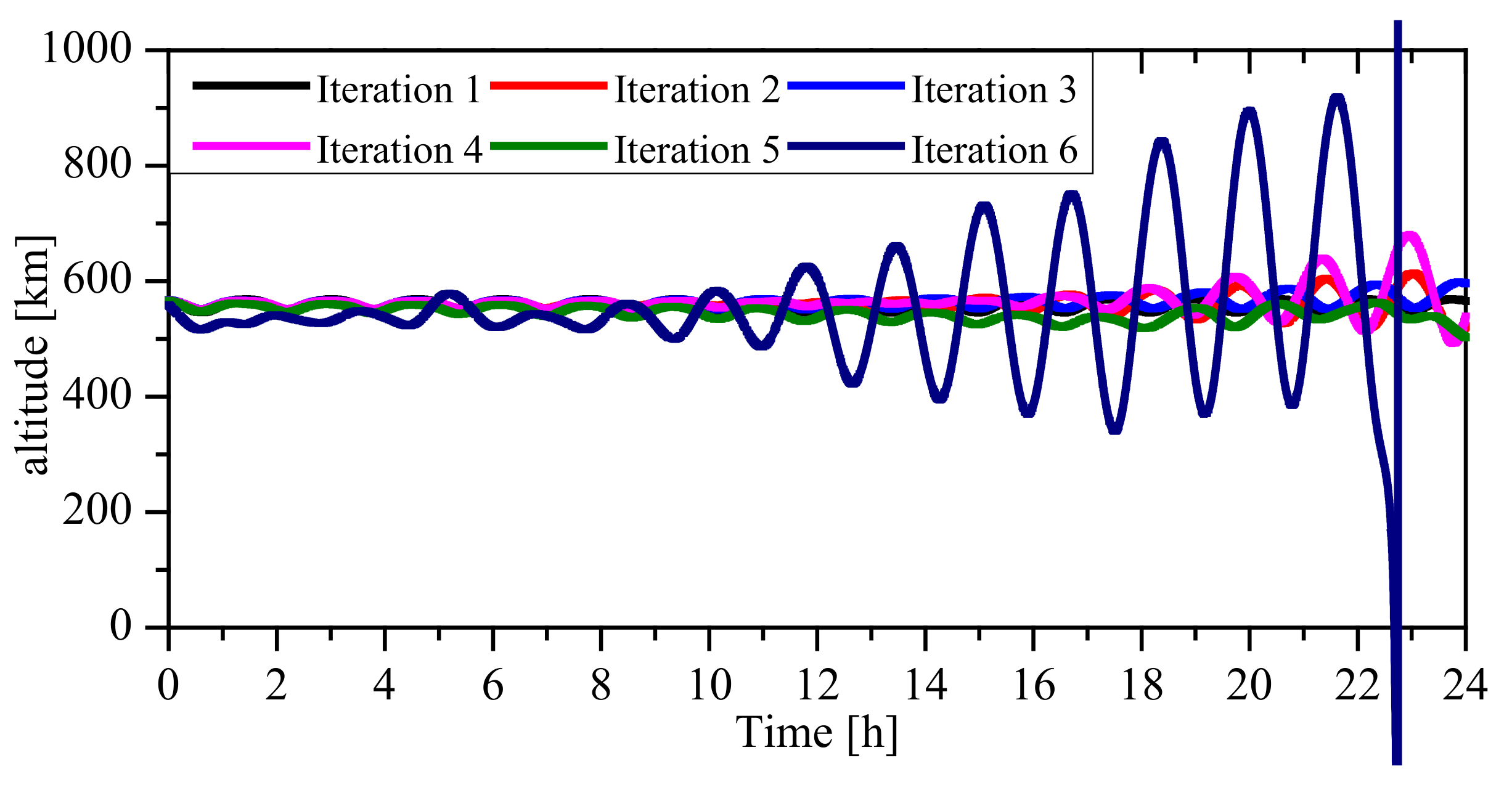
In order to analyze the divergent process in the direct approach, taking the orbit initialization experiment of KOMPSAT-5 on 2016/50 as an example, the position errors in the radial (R), along-track(T) and cross(N) directions and the 3D position error after each iteration step of the orbit parameter estimation are listed in Table 3. As can be observed clearly, the position error is increasing until the estimation diverges in the 6-th iteration, when the estimation iteration process proceeds. After the 5-th iteration, the 3D position error has been more than 50 km, which is a sign that the estimated orbit of KOMPSAT-5 at the altitude of ~590 km is severely deviated from the true orbit, so in the 6-th iteration the orbit parameters cannot be estimated. Correspondingly, the estimated altitude of KOMPSAT-5 after each iteration step is shown in Figure 5. As can be seen, at the end of the 5-th iteration, an altitude deviation of more than 50 km is resulted, which causes divergence in the 6-th iteration with a negative altitude estimated. The orbit initialization experiment of KOMPSAT-5 on 2016/50 demonstrates that the direct approach is unreliable when the starting velocity has large errors.
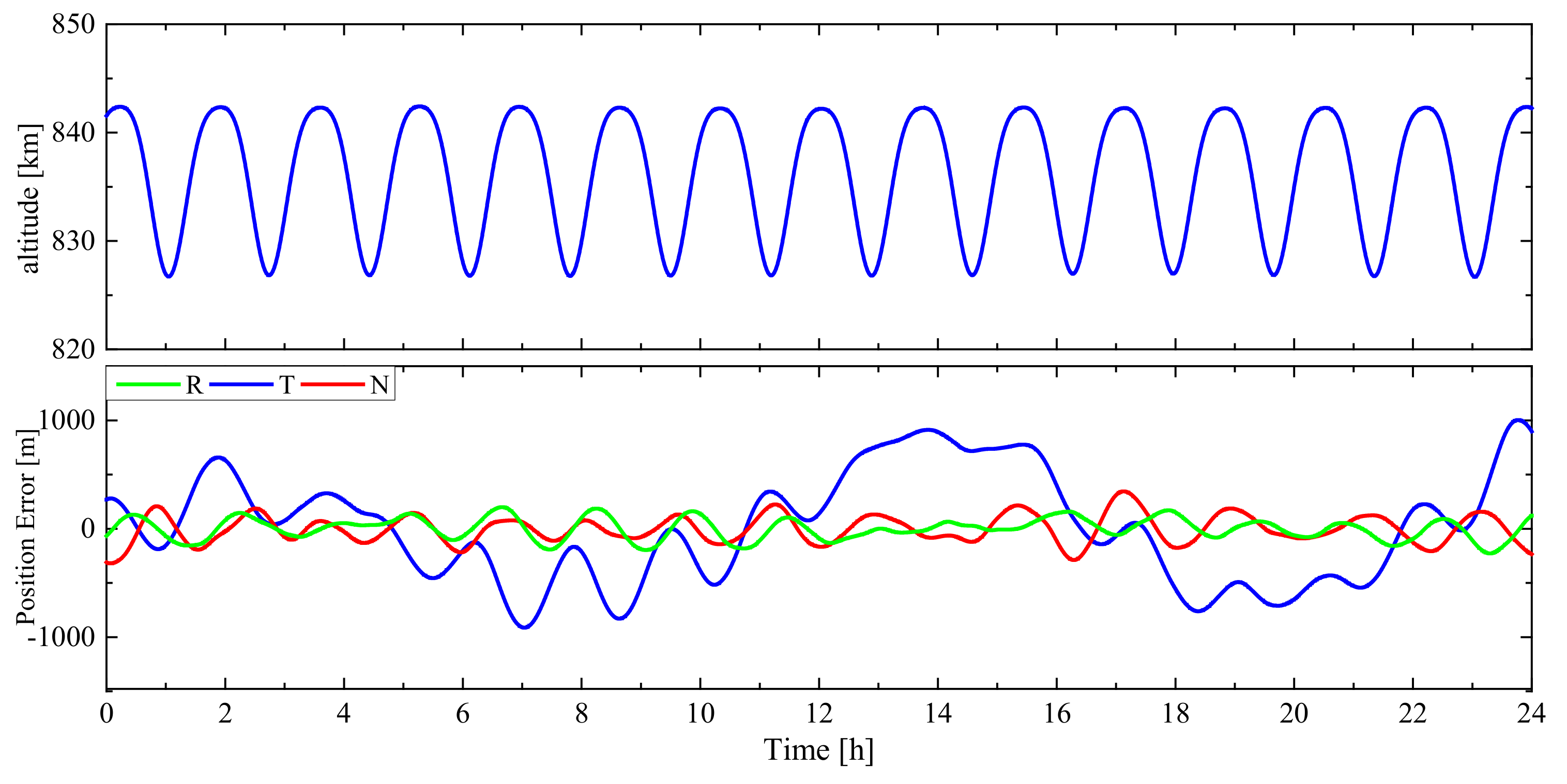
As for the progressive approach, the iterative estimation of parameters in reference ephemeris at step 2 is the key for the success of orbit initialization. The experiments above have demonstrated the high stability of the reference ephemeris estimation when facing with the starting velocity error of 1~10 m/s. To analyze its estimation process further, considering FY3C on 2013/287 as an example, the position differences in R/T/N directions between the reference orbit obtained at step 2 and the precise orbit are shown in Figure 6. As can be observed clearly, the position error of the reference orbit is within the range of ±1000 m and varies smoothly and continuously. The corresponding altitude also varies smoothly and periodically between 825 km and 845 km, which indicates the estimated reference orbit is sufficiently close to the true orbit. It is based on the smooth, continuous reference orbit that the estimation of orbit parameters X1 at step 4 could be performed well, although the position error is still at 500 m level. The estimation at step 5 uses the resulting orbit parameters at step 4 as the starting state and the raw SPP/PPP discrete kinematic positions as measurements. The accuracy of the starting state is accurate enough for convergence of the estimation at step 5. All in all, the progressive approach is more reliable then the direct approach for orbit initialization.
5. Summary and Conclusions
The sufficiently accurate and stable orbit initialization is an important prerequisite for LEO precise orbit determination using GNSS. This paper presents two orbit initialization methods, including the traditional direct approach and the proposed progressive approach. In the direct approach, the orbit parameters, including the position and velocity vector at the reference time and all piecewise dynamic coefficients, are estimated directly and iteratively from the SPP/PPP discrete kinematic positions. The analysis tests on the stability have demonstrated that the orbit parameters estimation is at the risk of divergence, which is mainly caused by the oversized starting velocity error, which may be difficult to prevent completely, because many factors could cause the inaccurate GNSS pseudo-range or Doppler measurements at the reference epoch, including the weak signal, tracking interruption, ionospheric disturbances, abnormal antenna, etc. Hence, the progressive approach is proposed to eliminate or weaken the risk of POD divergence, where the reference ephemeris in form of the parameters in GNSS broadcast ephemeris, instead of the conventional orbit parameters, are estimated from the SPP/PPP discrete positions first. The estimated reference ephemeris is then used to generate a series of tabular positions and velocities with the position error of hundreds or thousands of meters, indicating that the reference orbit is sufficiently close to the true orbit. Then, these tabular positions and velocities can be used as measurements to estimate the orbit parameters by using the direct approach. Finally, the generated orbit parameters are used as the starting state for the next direct estimation, and then more accurate orbit parameters can be determined. The stability analysis tests have validated that, the starting state error, especially the oversized starting velocity error, has less negative effect on the estimated reference ephemeris than on the orbit parameters, so the progressive approach is more stable and reliable than the direct approach.
The orbit initialization experiments are carried out for the KOMPSAT-5 and FY3C missions. The experiment results show that the initialization process fails on some days if using the direct approach, but the initial orbit parameters can be generated reliably on these days using the progressive approach. It indicates that the proposed progressive approach is more reliable and adaptable for LEO precise orbit determination, especially for the automated orbit determination of LEO satellites in a large-scale constellation.
Author Contributions
In this study, X.G. and J.S. designed the algorithm, performed experiments, analyzed data and wrote this paper. F.W. designed the software, performed experiments and edited the manuscript. X.L. supervised its analysis and edited the manuscript. All authors have read and agreed to the published version of the manuscript.
Funding
This research was funded by National Natural Science Foundation of China (Nos. 91638203) and China Postdoctoral Science Foundation (Nos. 2020M682479).
Acknowledgments
The numerical calculations in this paper have been done on the supercomputing system in the Supercomputing Center of Wuhan University(WHU). Thanks a lot for the support of Supercomputing Center of WHU.
Conflicts of Interest
The authors declare no conflict of interest.
References
- Montenbruck, O.; Ramos-Bosch, P. Precision real-time navigation of LEO satellites using global positioning system measurements. GPS Solut. 2008, 12, 187–198. [Google Scholar] [CrossRef]
- Wang, F.; Gong, X.; Sang, J.; Zhang, X. A novel method for precise onboard real-time orbit determination with a standalone GPS receiver. Sensors 2015, 15, 30403–34018. [Google Scholar] [CrossRef] [PubMed] [Green Version]
- Jérôme, L. The Use of GPS/GNSS on Earth and in Space; Montreal Space Symposium: Montreal, QC, Canada, 2018. [Google Scholar]
- Montenbruck, O.; Hackel, S.; Jäggi, A. Precise orbit determination of the Sentinel-3A altimetry satellite using ambiguity-fixed GPS carrier phase observations. J. Geod. 2018, 92, 711–726. [Google Scholar] [CrossRef] [Green Version]
- Li, X.; Zhang, K.; Meng, X.; Zhang, W.; Zhang, Q.; Zhang, X.; Li, X. Precise orbit determination for the FY-3C satellite using onboard BDS and GPS observations from 2013, 2015, and 2017. Engineering 2019. [Google Scholar] [CrossRef]
- Li, X.; Wu, J.; Zhang, K.; Li, X.; Xiong, Y.; Zhang, Q. Real-Time kinematic precise orbit determination for LEO satellites using zero-differenced ambiguity resolution. Remote Sens. 2019, 11, 2815. [Google Scholar] [CrossRef] [Green Version]
- Gooding, R.H. A New Procedure for Orbit Determination Based on Three Lines of Sight (Angles Only); Defence Research Agency Farnborough: Hampshire, UK, 1993.
- Fujimoto, K.; Scheeres, D.J. Short-arc correlation and initial orbit determination for space-based observations. In Proceedings of the 2011 Advanced Maui Optical and Space Surveillance Technologies Conference, Maui, HI, USA, 13–16 September 2011. [Google Scholar]
- Weisman, R.M.; Majji, M.; Alfriend, K.T. Analytic characterization of measurement uncertainty and initial orbit determination on orbital element representations. Celest. Mech. Dyn. Astron. 2014, 118, 165–195. [Google Scholar] [CrossRef]
- Lei, X.; Wang, K.; Zhang, P.; Pan, T.; Li, H.; Sang, J.; He, D. A geometrical approach to association of space-based very short-arc LEO tracks. Adv. Space Res. 2018, 62, 542–553. [Google Scholar] [CrossRef]
- Li, X.; Ma, F.; Li, X.; Lv, H.; Bian, L.; Jiang, Z.; Zhang, X. LEO constellation-augmented multi-GNSS for rapid PPP convergence. J. Geod. 2019, 93, 749–764. [Google Scholar] [CrossRef]
- Ardito, C.T.; Morales, J.J.; Khalife, J.; Abdallah, A.A.; Kassas, Z. Performance evaluation of navigation using LEO satellite signals with periodically transmitted satellite positions. In Proceedings of the 2019 International Technical Meeting of The Institute of Navigation, Reston, VA, USA, 28–31 January 2019; pp. 306–318. [Google Scholar]
- Wang, L.; Chen, R.; Xu, B.; Zhang, X.; Li, T.; Wu, C. The challenges of LEO based navigation augmentation system–lessons learned from Luojia-1A satellite. In Proceedings of the China Satellite Navigation Conference (CSNC) 2019 Proceedings, Beijing, China, 22–25 May 2019; pp. 298–310. [Google Scholar]
- Li, X.; Zhang, K.; Ma, F.; Zhang, W.; Zhang, Q.; Qin, Y.; Zhang, H.; Meng, Y.; Bian, L. Integrated precise orbit determination of multi-GNSS and large LEO constellations. Remote Sens. 2019, 11, 2514. [Google Scholar] [CrossRef] [Green Version]
- Li, X.; Zhang, K.; Meng, X.; Zhang, Q.; Zhang, W.; Li, X.; Yuan, Y. LEO–BDS–GPS integrated precise orbit modeling using FengYun-3D, FengYun-3C onboard and ground observations. GPS Solut. 2020, 24, 1–13. [Google Scholar] [CrossRef]
- Borio, D.; Sokolova, N.; Lachapelle, G. Doppler measurements and velocity estimation: A theoretical framework with software receiver implementation. In Proceedings of the ION GNSS 2009, Savannah, GA, USA, 23–25 September 2009; pp. 23–25. [Google Scholar]
- Colombo, O.L. The dynamics of Global Positioning System orbits and the determination of precise ephemerides. J. Geophys. Res. 1989, 94, 9167–9182. [Google Scholar] [CrossRef]
- Montenbruck, O.; Gill, E. Satellite Orbits: Models, Methods and Application; Springer: Berlin/Heidelberg, Germany, 2000. [Google Scholar]
- Anthony Flores, R.E. NAVSTAR GPS Space Segment/Navigation User Segment Interfaces (IS-GPS-200L). 2020. Available online: https://www.gps.gov/technical/icwg/IS-GPS-200L.pdf (accessed on 14 May 2020).
- Fu, X.; Wu, M. Optimal design of broadcast ephemeris parameters for a navigation satellite system. GPS Solut. 2012, 16, 439–448. [Google Scholar] [CrossRef]
- Földváry, L. Determination of satellite velocity and acceleration from kinematic LEO orbits. Acta Geod. Geophys. Hung. 2007, 42, 399–419. [Google Scholar] [CrossRef]
- Hwang, Y.; Lee, B.S.; Kim, Y.R.; Roh, K.M.; Jung, O.C.; Kim, H. GPS-based orbit determination for KOMPSAT-5 satellite. ETRI J. 2011, 33, 487–496. [Google Scholar] [CrossRef]
- Li, M.; Li, W.; Shi, C.; Jiang, K.; Guo, X.; Dai, X.; Meng, X.; Yang, Z.; Yang, G.; Liao, M. Precise orbit determination of the Fengyun-3C satellite using onboard GPS and BDS observations. J. Geod. 2017, 91, 1313–1327. [Google Scholar] [CrossRef] [Green Version]
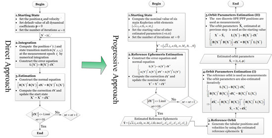
Figure 1.
The iterative estimation scheme of the direct approach.

Figure 2.
The estimation scheme of the progressive approach.

Figure 3.
The design errors due to starting state errors in orbit parameters estimation.


Figure 4.
The design errors due to the starting state error in reference ephemeris estimation.

Figure 5.
The estimated altitude of KOMPSAT-5 after each iteration step of orbit parameter estimation by direct approach.
Figure 5.
The estimated altitude of KOMPSAT-5 after each iteration step of orbit parameter estimation by direct approach.

Figure 6.
The altitude and position error of the reference orbit of FY3C on 2013/287.


Table 1.
The daily status of orbit initialization experiments of KOMPSAT-5 and FY3C.
| Date | KOMPSAT-5 | Date | FY3C | ||
|---|---|---|---|---|---|
| DA | PA | DA | PA | ||
| 2016/42 | √ | √ | 2013/285 | √ | √ |
| 2016/43 | × | √ | 2013/286 | √ | √ |
| 2016/44 | × | √ | 2013/287 | × | √ |
| 2016/45 | × | √ | 2013/288 | × | √ |
| 2016/46 | √ | √ | 2013/289 | √ | √ |
| 2016/47 | √ | √ | 2013/290 | √ | √ |
| 2016/48 | √ | √ | 2013/291 | √ | √ |
| 2016/49 | × | √ | 2013/292 | √ | √ |
| 2016/50 | × | √ | 2013/293 | √ | √ |
| 2016/51 | √ | √ | 2013/294 | √ | √ |
Table 2.
The position error statistics during the iterative process with the direct and progressive approaches.
Table 2.
The position error statistics during the iterative process with the direct and progressive approaches.
| Iterations | KOMPSAT-5 | FY3C | ||||||
|---|---|---|---|---|---|---|---|---|
| 2016/43 | 2016/44 | 2016/45 | 2016/49 | 2016/50 | 2013/287 | 2013/288 | ||
| Mean position error/m | 1.37 | 3.23 | 1.97 | 2.55 | 1.42 | 2.13 | 1.66 | |
| Mean velocity error/m/s | 2.73 | 2.44 | 2.43 | 3.67 | 1.95 | 2.85 | 1.76 | |
| DA/m | 1 | 64,450.8 | 20,124.5 | 2229.1 | 8672.6 | 3186.9 | 194,731.9 | 151,436.3 |
| 2 | 187,660.3 | Diverge | 5358.6 | 45,891.1 | 2282.1 | Diverge | 352,364.8 | |
| 3 | Diverge | 21,577.4 | Diverge | 3774.3 | Diverge | |||
| 4 | Diverge | 13,163.1 | ||||||
| 5 | 51,953.5 | |||||||
| 6 | Diverge | |||||||
| PA/m | 2.1 | 18,653.5 | 47,787.9 | 81,857.9 | 49,213.3 | 18,536.2 | 19,918.5 | 51,806.7 |
| 2.2 | 562.3 | 567.7 | 885.56 | 573.0 | 564.6 | 532.0 | 525.0 | |
| 2.3 | 562.4 | 575.1 | 1124.2 | 581.7 | 564.7 | 532.1 | 534.8 | |
| 2.4 | 562.4 | 563.1 | 566.4 | 566.8 | 564.6 | 532.0 | 518.4 | |
| 2.5 | 562.4 | 563.1 | 566.4 | 566.8 | 564.6 | 532.0 | 518.4 | |
| 4.1 | 540.5 | 488.9 | 439.2 | 508.4 | 456.5 | 498.8 | 491.6 | |
| 4.2 | 540.5 | 488.7 | 435.9 | 508.2 | 456.7 | 498.8 | 491.7 | |
| 4.3 | 540.5 | 488.7 | 435.8 | 508.2 | 456.7 | 498.8 | 491.7 | |
| 5.1 | 5.6 | 5.4 | 6.1 | 7.3 | 6.1 | 12.5 | 10.5 | |
| 5.2 | 5.6 | 5.4 | 6.1 | 7.3 | 6.1 | 12.5 | 10.5 | |
| 5.3 | 5.6 | 5.4 | 6.1 | 7.3 | 6.1 | 12.5 | 10.5 | |
Table 3.
The R/A/C/3D position errors after each iteration step of orbit parameter estimation by the direct approach.
Table 3.
The R/A/C/3D position errors after each iteration step of orbit parameter estimation by the direct approach.
| Iterations | R/m | T/m | N/m | 3D/m |
|---|---|---|---|---|
| 1 | 3137.55 | 558.00 | 20.98 | 3186.85 |
| 2 | 2199.16 | 608.68 | 32.88 | 2282.07 |
| 3 | 3623.94 | 1054.26 | 29.63 | 3774.29 |
| 4 | 12,550.51 | 3967.17 | 120.29 | 13,163.14 |
| 5 | 51,131.22 | 9198.94 | 373.86 | 51,953.46 |
| 6 | Diverge... | |||
Publisher’s Note: MDPI stays neutral with regard to jurisdictional claims in published maps and institutional affiliations. |
© 2020 by the authors. Licensee MDPI, Basel, Switzerland. This article is an open access article distributed under the terms and conditions of the Creative Commons Attribution (CC BY) license (http://creativecommons.org/licenses/by/4.0/).
Share and Cite
MDPI and ACS Style
Gong, X.; Sang, J.; Wang, F.; Li, X. A More Reliable Orbit Initialization Method for LEO Precise Orbit Determination Using GNSS. Remote Sens. 2020, 12, 3646. https://0-doi-org.brum.beds.ac.uk/10.3390/rs12213646
AMA Style
Gong X, Sang J, Wang F, Li X. A More Reliable Orbit Initialization Method for LEO Precise Orbit Determination Using GNSS. Remote Sensing. 2020; 12(21):3646. https://0-doi-org.brum.beds.ac.uk/10.3390/rs12213646
Chicago/Turabian StyleGong, Xuewen, Jizhang Sang, Fuhong Wang, and Xingxing Li. 2020. "A More Reliable Orbit Initialization Method for LEO Precise Orbit Determination Using GNSS" Remote Sensing 12, no. 21: 3646. https://0-doi-org.brum.beds.ac.uk/10.3390/rs12213646
Note that from the first issue of 2016, this journal uses article numbers instead of page numbers. See further details here.