Improving Stage–Discharge Relation in The Mekong River Estuary by Remotely Sensed Long-Period Ocean Tides


1
School of Geodesy and Geomatics, Wuhan University, Wuhan 430079, China
2
Key Laboratory of Geophysical Geodesy, Ministry of Natural Resources, Wuhan 430079, China
3
Institute of Marine Science and Technology, Wuhan University, Wuhan 430079, China
4
Department of Civil, Environmental and Geodetic Engineering, Ohio State University, Columbus, OH 43210, USA
5
Core Faculty, Translational Data Analytics Institute, Ohio State University, Columbus, OH 43210, USA
*
Author to whom correspondence should be addressed.
Remote Sens. 2020, 12(21), 3648; https://0-doi-org.brum.beds.ac.uk/10.3390/rs12213648
Submission received: 6 October 2020
/
Revised: 28 October 2020
/
Accepted: 5 November 2020
/
Published: 6 November 2020
(This article belongs to the Special Issue Coastal Waters Monitoring Using Remote Sensing Technology)
Abstract
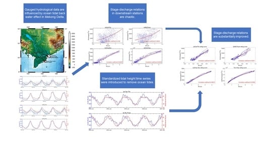
:Ocean tidal backwater reshapes the stage–discharge relation in the fluvial-to-marine transition zone at estuaries, rendering the cautious use of these data for hydrological studies. While a qualitative explanation is traditionally provided by examining a scatter plot of water discharge against water level, a quantitative assessment of long-period ocean tidal effect on the stage–discharge relation has been rarely investigated. This study analyzes the relationship among water level, water discharge, and ocean tidal height via their standardized forms in the Mekong Delta. We found that semiannual and annual components of ocean tides contribute significantly to the discrepancy between standardized water level and standardized water discharge time series. This reveals that the long-period ocean tides are the significant factors influencing the stage–discharge relation in the river delta, implying a potential of improving the relation as long as proper long-period ocean tidal components are taken into consideration. By isolating the short-period signals (i.e., less than 15 days) from land surface hydrology and ocean tides, better consistent stage–discharge relations are obtained, in terms of improving the Pearson correlation coefficient (PCC) from ~0.4 to ~0.8 and from ~0.6 to ~0.9 for the stations closest to the estuary and at the Mekong Delta entrance, respectively. By incorporating the long-period ocean tidal height time series generated from a remotely sensed global ocean tide model into the stage–discharge relation, further refined stage–discharge relations are obtained with the PCC higher than 0.9 for all employed stations, suggesting the improvement of daily averaged water level and water discharge while ignoring the short-period intratidal variability. The remotely sensed global ocean tide model, OSU12, which contains annual and semiannual ocean tide components, is capable of generating accurate tidal height time series necessary for the partial recovery of the stage–discharge relation.
1. Introduction
Accurate water level (WL) and water discharge (WD) measurements are fundamental to various hydrological applications, including flood forecasting, design and operation of conservancy facilities, as well as water and sediment budget analyses [1,2]. However, due to economy, politics, and topography along a river [3], the spatial distribution of hydrological stations is both sparse and uneven, along with inconsistent and missing datasets [4]. In order to complement the above deficiency of observed datasets, it is a common practice to extend the datasets both in space and time by converting one type of data into another, for instance, estimating WD from WL.
The conversion between WL and WD is referred to as the stage–discharge relation. Under a pure hydrological situation, this relation is represented by a power function, also called rating curve. There are two available methods to obtain the stage–discharge relation. The first method is based on numerical solutions of dynamic models [5,6,7] that simulates the stage–discharge relation when accurate hydraulic geometry and boundary conditions are available. The second method is based on data-driven models that can be based on the power function fitting, non-linear regression techniques [8,9,10], or an artificial neural network (ANN) [11,12,13,14].
In essence, WD is not only related to WL alone, but also disturbed by water surface slope, channel geometry, bed roughness, flow unsteadiness, lateral flow, and the backwater effect caused by an ocean tidal wave propagating up to estuaries [15,16]. Therefore, the stage–discharge relation becomes more complicated, manifesting as multiple loops [17]. In the river delta, the influence of the ocean tidal wave is a significant factor that distorts the well-established stage–discharge relation [8]. Consequently, the WL and WD data near the estuary mouth at river deltas are used cautiously for research studies, as those data are contaminated by the aforementioned factors. For instance, Sassi et al. [18] quantitatively analyses the contribution of different ocean tidal components (i.e., quarter-diurnal, semidiurnal, diurnal, and fortnightly) to surface water variation. The fluvial-to-marine transition zone of Mekong Delta have been further subdivided into four sections (i.e., fluvial-dominated tide-affected, fluvial-dominated tide-influenced, tide-dominated fluvial-influenced, and tide-dominated fluvial-affected zones), according to salinity, channel morphology, fades/grain size, and the extent of ocean tidal influence by Gugliotta et al. [19]. However, the stage–discharge relation at the river delta corrected by ocean tidal components remains unexplored.
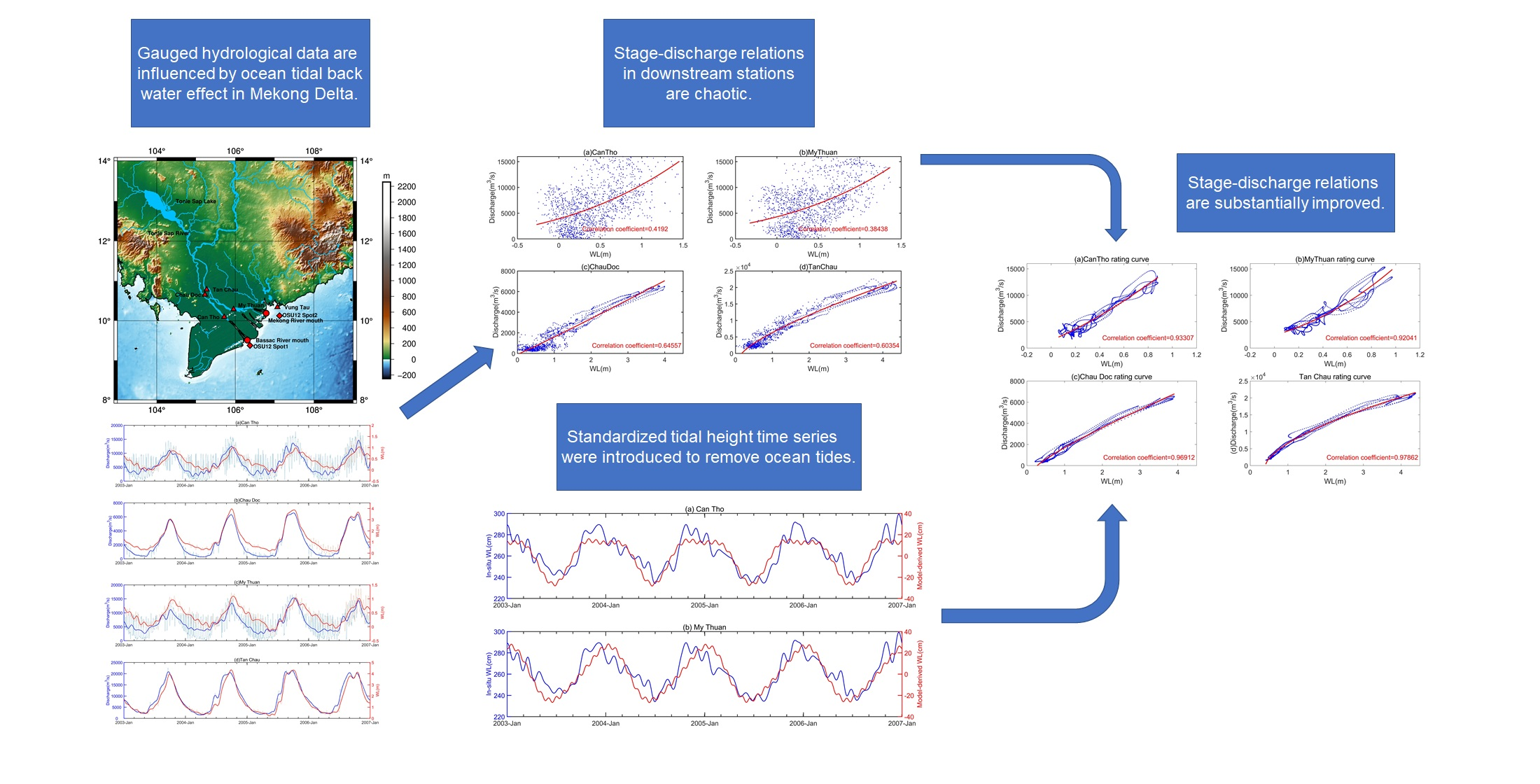
The Mekong Delta (MD) (Figure 1), being home to 19 million people, is an important agricultural and fishing district in Southeast Asia [17,20]. Further anthropogenic stressors are massive river training and construction of a multitude of large hydropower dams and severe sand extraction for concrete production [21,22,23]. This is characterized by a relatively flat surface with low altitudes and gradients [24,25]. Being a transition zone, WD and WL variability are dynamically affected by both fluvial and marine processes seasonally [26,27]. As a result, reverse flow caused by ocean tidal wave and storm surge can easily propagate along river channels [8]. As a result, salinity intrusion and catastrophic flooding along with rising sea level [28,29,30] severely threaten the grain production in the MD [31,32]. This also affects hydrological gauge stations within a distance of 200 kilometers away from the estuary mouth. In addition, the Tonle Sap Lake in Cambodia also provides a regulation effect [33,34,35], before the river runoff delivers to the MD and discharges eventually to the South China Sea through the Bassac River and the Mekong river within the MD [36]. As a consequence, the stage–discharge relation in this region exhibits multiple looping curves along with noisy patterns [33,37].
Despite qualitative explanations, the ocean tidal backwater effect has not been quantified and corrected for. After all, the complex interaction between oceanic and fluvial processes is a cross-disciplinary science among land surface hydrology, estuary, and ocean science. As long as an appropriate method can be introduced to partially recover the stage–discharge relation with good accuracy, the corrected data would be of great usage. For such a purpose, the analysis of the disturbance of the stage–discharge relation by different components of ocean tides, based on a tidal data analysis or a remotely-sensed global ocean tide model, is a prerequisite.
This study aims to demonstrate the potential of incorporating the ocean tidal components into the stage–discharge relation for a partial relation recovery in the MD. The relation among WD, WL, and ocean tidal height data time series are analyzed via their standardized forms. The ocean tidal components generated from remotely sensed OSU12 global ocean tide model are substituted into the resulting model relation generated from the analysis. The fitted model relation is subsequently applied for estimating WD from ocean tidal height and WL. A quantitative evaluation of the estimated WD against the observed hydrological data is also presented.
2. Datasets and Assessment Metrics
In this study, in-situ data from hydrological stations, tidal gauge data, and OSU12 global ocean tide model were analyzed. Table 1 summarizes the essential information about these datasets.
2.1. In-Situ Hydrological Data
Station data time series within the MD were obtained from the Mekong River Commission (MRC) (http://www.mrcmekong.org). Acoustic Doppler Current Profiler (ADCP) was applied to gauge flow velocity for deriving precise discharge, according to MRC [39]. To compare between the two main subdivided branches within the MD, Tan Chau and My Thuan stations along the Mekong River, and Chau Doc and Can Tho stations along the Bassac River were used. Situated at the entrance of the MD [27], the Tan Chau and Chau Doc stations are, respectively, ~220 and ~240 km away from the estuary mouth. Both stations are in the middle between the Tonle Sap Lake and the estuary mouth, where the regulation effect of the lake and the ocean tidal backwater effect are minimized. Being the closest hydrological stations to the estuary mouth, My Thuan and Can Tho stations are subject to the backwater effect caused by landward ocean tidal propagation, which is clearly shown in the data time series [27]. Hence, the comparison between upper and lower station pairs allows us to further quantify the extent of the ocean tidal backwater effect.
Note that WD data of Tan Chau station were missing in 2001, 2002, and 2007. To be consistent with the time span of other WD data, the station time series spanning from January 2003 to December 2006 were selected for investigation, while those from January 2009 to December 2014 were employed for validation. Given the different temporal resolutions among WL, WD, and in-situ ocean tidal data time series and in order to isolate signals unrelated to hydrology, a Butterworth filter was applied to these time series for suppressing periodic fluctuations shorter than 15 days (e.g., diurnal, semidiurnal, etc.). The mean, maximum, and minimum values of those time series are summarized in Table 2.
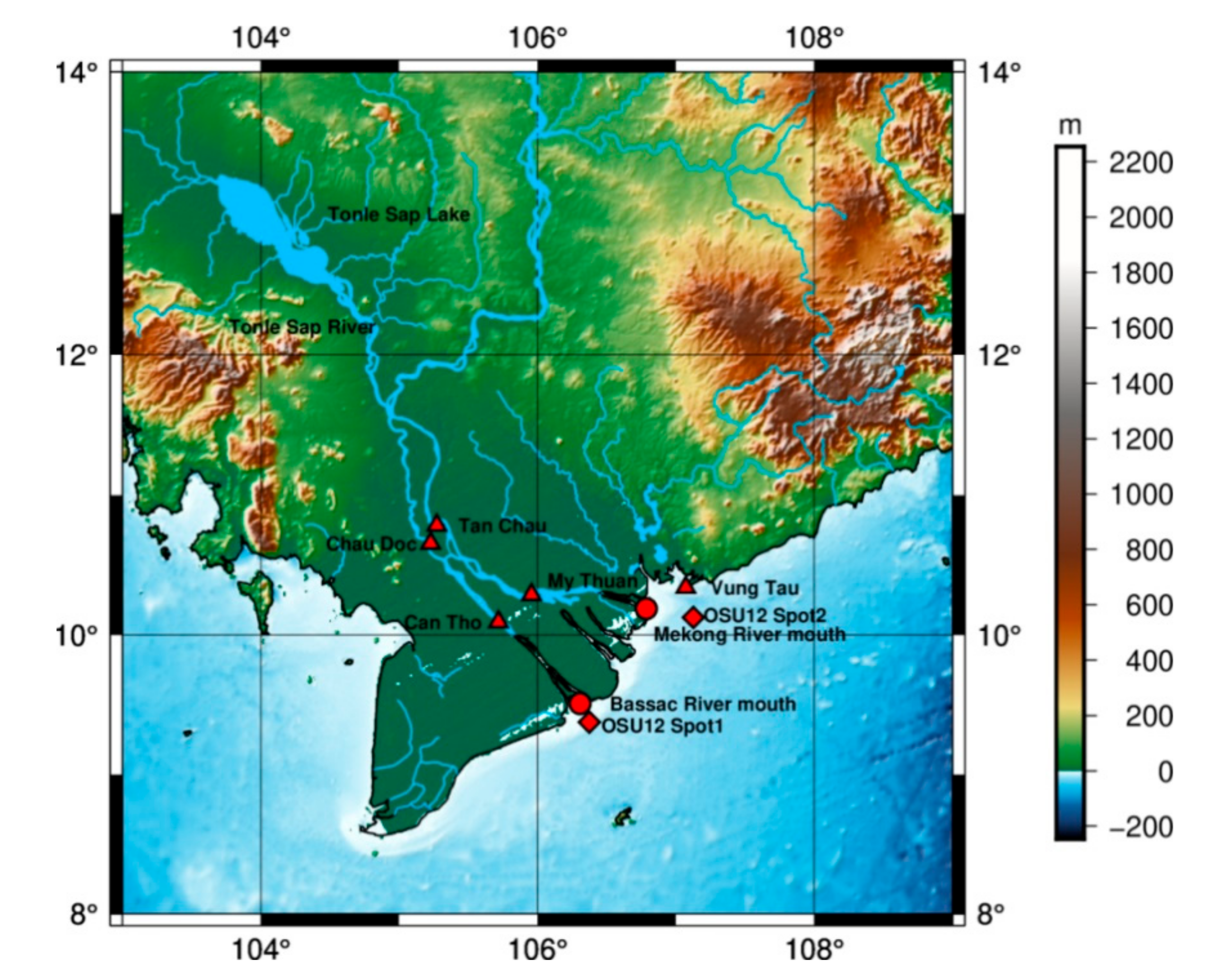
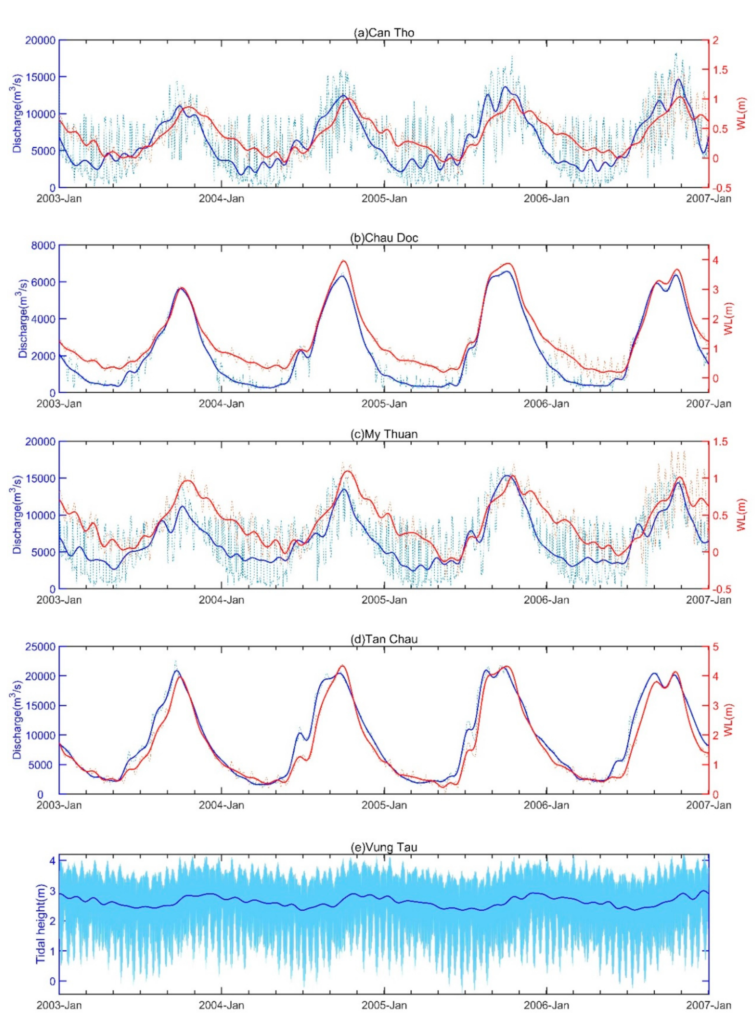
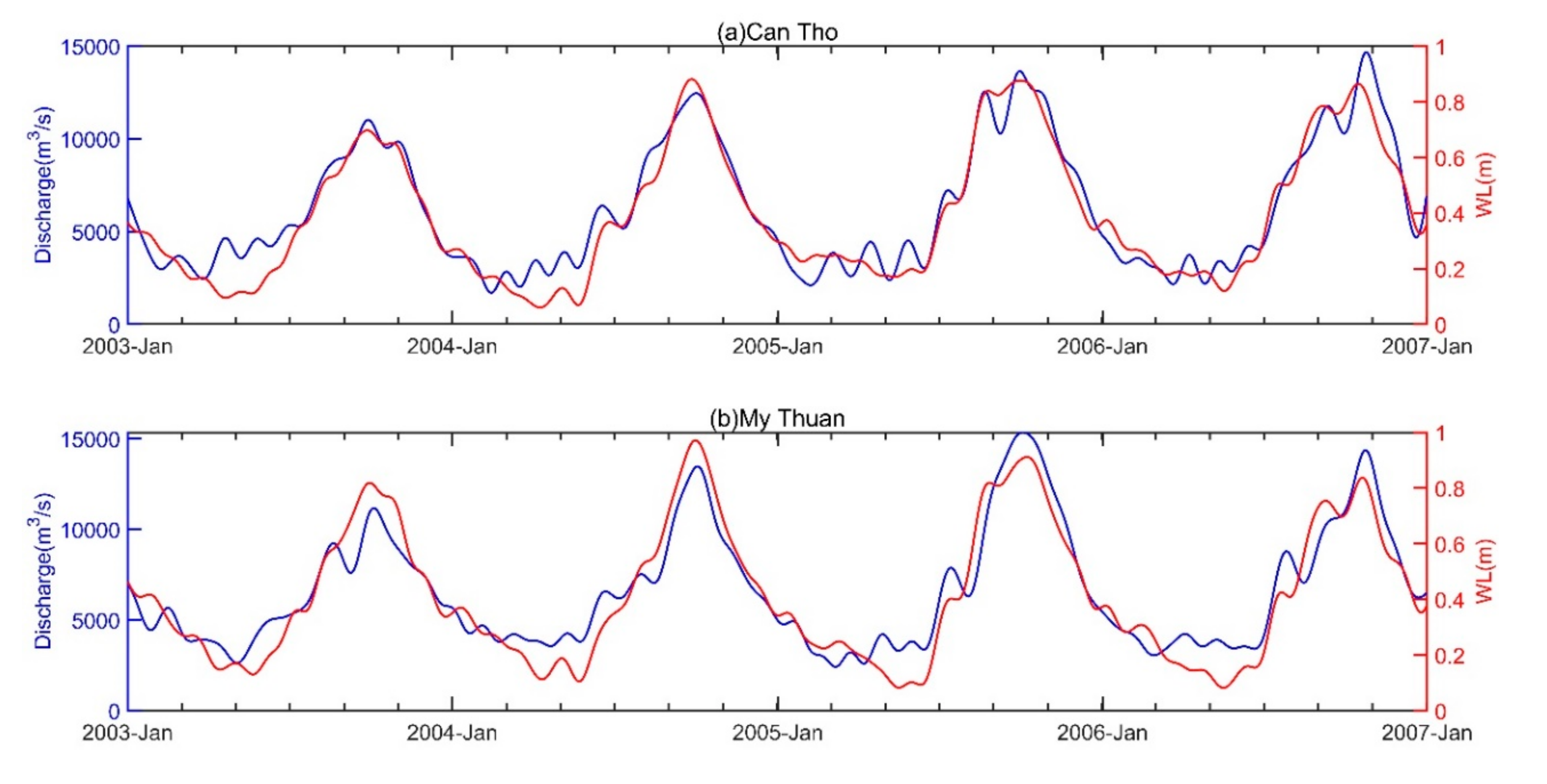
Filtered and original time series of the four stations are displayed, showing common characteristics of the WL and WD time series along with their differences (Figure 2a–d). Can Tho and My Thuan station time series show a larger ocean tide backwater effect than those of Chau Doc and Tan Chau stations. By comparing WL with WD time series, WD lags behind WL by approximately a month. This fact is more pronounced for stations closer to the estuary mouth (i.e., Can Tho and My Thuan) than their upper counterparts (i.e., Chau Doc and Tan Chau). Obviously, the annual signal is apparent for all station time series, in which the temporal patterns are highly related to not only seasonal variation of watershed runoff, but also the long-period (e.g., semiannual and annual) ocean tidal components, as shown in Figure 2e. As a consequence, external information obtained from the tide gauge or ocean tide model data near estuaries can be potentially used for removing the effect of long-period ocean tidal components, which is the objective of this study.
2.2. Sea Level Data from Tide Gauge Station
A tide gauge measures sea level time series at selected locations along the coasts [40]. Vung Tau is the closest tide gauge station to Mekong estuary chosen for relating the long-period ocean tidal variation to WL within the MD. Spanning from 2003 to 2014, the sea level time series at Vung Tau station were recorded on an hourly interval. This dataset is provided by the Hydrological and Environmental station network center in Vietnam and can be obtained from http://www.ioc-sealevelmonitoring.org/station.php?code=vung.
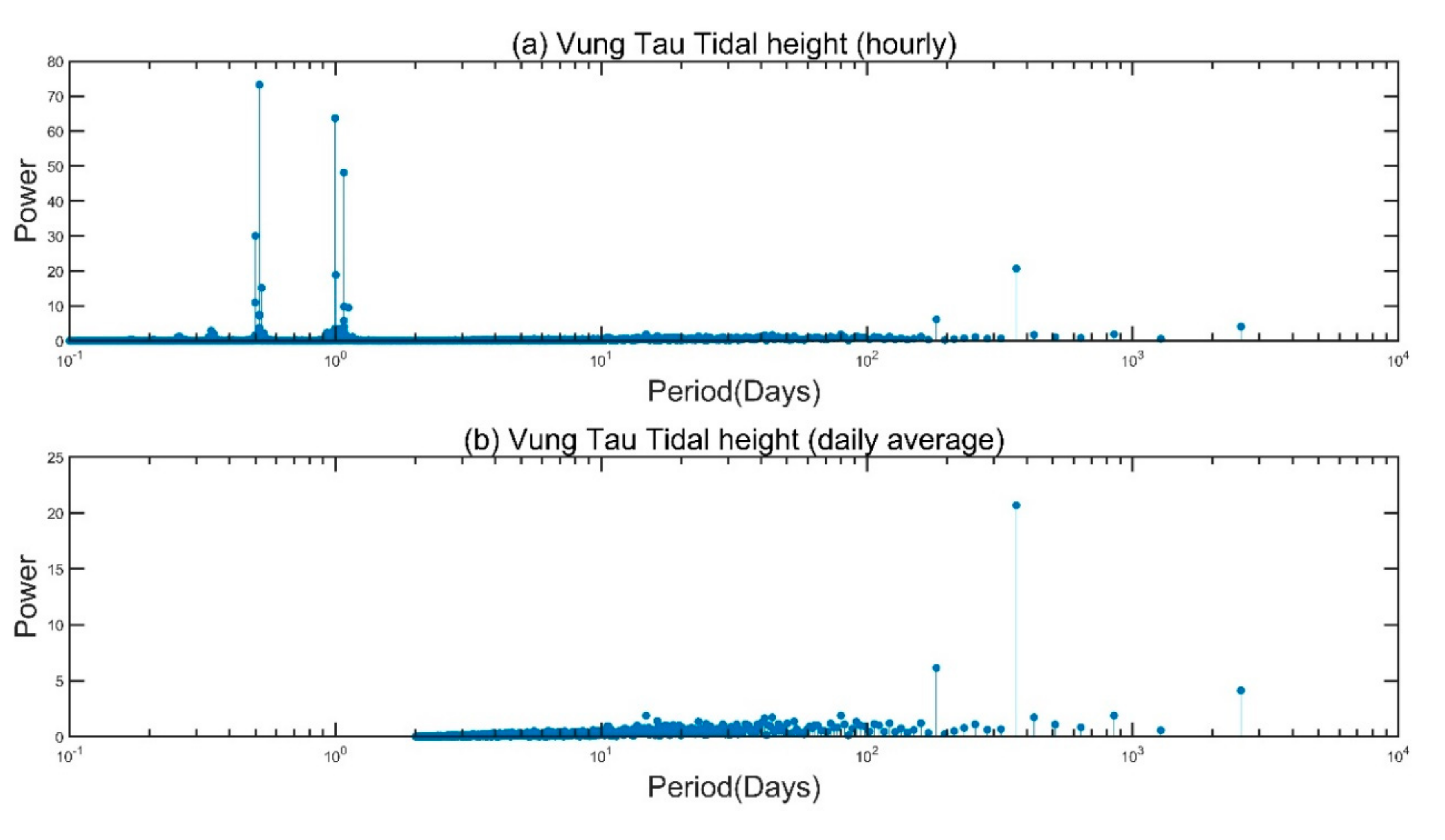
Figure 2e shows filtered and original hourly time series of the tidal gauge data. Fast Fourier transform (FFT) was applied to identify different periodic components of the time series. The highest power spectra are located at both diurnal and semidiurnal ocean tidal components (Figure 3a), which are unrelated to hydrological signals. In order to be consistent with WD and WL time series’ daily sampling rate, the hourly tidal height time series are averaged daily after filtering high-frequency components via the Butterworth filter. This process, to a large extent, suppresses or removes the short-period ocean tidal components via the low-pass filtering process, and hence, reducing the effect on long-term ocean tidal components [41,42,43] (Figure 3b). Compared with the unfiltered time series, only semiannual and annual tide components are apparent in the processed time series.
2.3. Global Ocean Tide Model Data
A global ocean tide model contains gridded in-phase and quadrature amplitudes (or equivalently amplitude and phase) for major tidal constituents, allowing us to generate ocean tidal height in the absence of tide gauge stations along the coasts [44,45]. Although many remotely sensed ocean tide models (e.g., FES2014, GOT4.8, NAO99.b, TPXO8, EOT11a, DTU10, HAMTIDE, OSU12, etc.) are available for the purpose of our study, the OSU12 model, with a 0.25° × 0.25° spatial resolution [46,47], was employed to generate long-period tidal height time series at grid points near Mekong and Bassac river estuaries (Table 3), because it contained long-period tides and was derived purely from remotely sensed satellite altimetry data. Notwithstanding smaller amplitude when compared with semidiurnal and diurnal tides, long-period ocean tidal components are influential to daily and monthly average WL time series. As shown in Figure 2 and Figure 3b, long-period ocean tidal components are likely related to the discrepancies between the pattern of WL and WD time series. It is appropriate to calculate the ocean tidal height time series, TH(t), at time t from the in-phase, H1, and quadrature amplitudes, H2, of Sa, Ssa, and Mm tides, which can be formulated as:
where Ti is the period of each long-period ocean tidal component i. Note that both the in-phase and quadrature amplitudes are with respect to Greenwich Meridian with the starting time, 0:00 AM, 1 January 2002 (UTC +0).
2.4. Assessment Metrics
To evaluate the estimated WD against in-situ WD time series in Section 4, three assessment metrics, R-Square, the Pearson correlation coefficient (PCC), and the Nash–Sutcliffe efficiency (NSE) coefficient, are employed.
R-Square, ranging between 0 and 1, describes how much the variation of in-situ WD, , is explained by the estimated WD, , generated from the model. The closer the value to 1, the better the model fitting to the . R-Square is equal to the quotient of sum of squares regression (SSR) divided by sum of squares total (SST), and can be defined as:
PCC, ranging between −1 and 1, describe how strong the linear relationship between and , which is defined as:
where and are the mean of and , respectively. Notably, for the power function relating WL to WD, logarithmic transform is applied to obtain the log-linear relation between the two variables in order to assess their correlation. To highlight the difference, PCC was used to represent the linear relationship between and , while “correlation coefficient” appeared in each figure of this study referred to the log-linear relation between WD and WL, as shown in Equation (6) below.
NSE coefficient, ranging from to 1, describes the gain in the performance of against . The closer the NSE coefficient to 1, the better the performance of the estimation [48]. It is defined as:
3. Data Analysis and Methodology
This section explores the relations among ocean tidal height, WL, and WD time series over our study region, so as to illustrate the interaction between fluvial and oceanic factors along with their combined effects on WL and WD data. For an ideal hydrological station location where WL and WD are purely influenced by the fluvial process, WL and WD are related by a power function [49] expressed as:
where , , c are the scaling coefficient, the offset of WL and the exponent of power function, respectively.
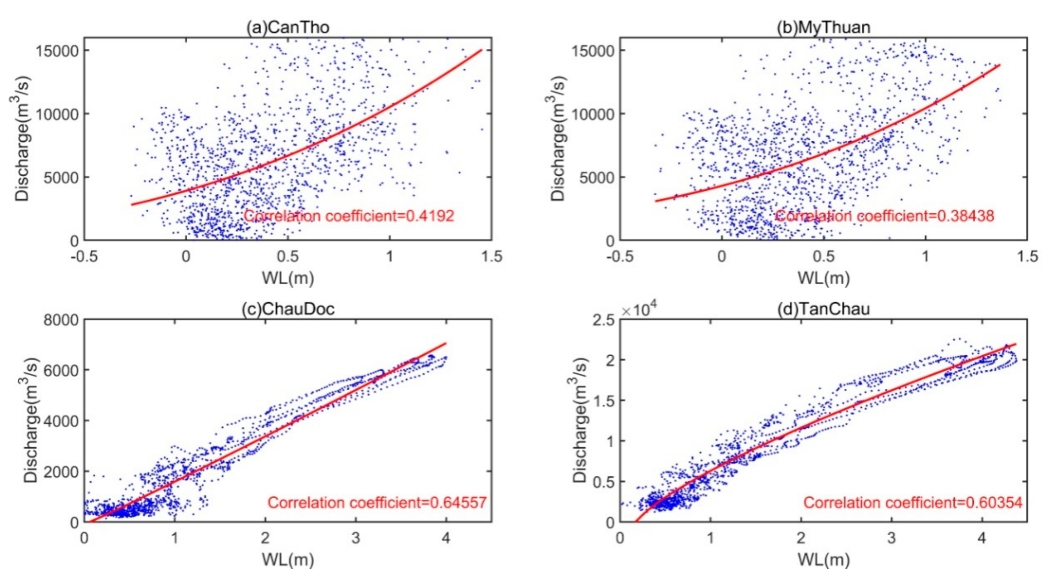
However, in reality, the stage–discharge phase diagram between WL and WD appears as random data points with trends (i.e., Can Tho and My Thuan stations) and elliptical curves (i.e., Chau Doc and Tan Chau stations) in the MD (Figure 4).
The logarithmic transform of Equation (5) allows the conversion into log-linear relation, expressed as:
such that Equation (6) measures a linear relationship between and . All “correlation coefficients” displayed in all stage–discharge phase diagrams were calculated based on and , as mentioned in Section 2.4.
Compared to those of the other two stations, the rating curves between WL and WD of Can Tho and My Thuan stations yield lower correlation coefficients because they are more significantly affected by the ocean tidal backwater.
3.1. Data Analysis of Backwater Influence on Water Discharge (WD) and Water Level (WL)
Although the phase diagram between WL and WD in the tide-dominated area appears elliptical, the patterns of the deviation from the rating curves are presumed to be analyzable by different ocean tidal components. Through FFT, the most pronounced periods are 365 days, 182.5 days, and 14.7475 days in both WD and WL time series.
The relative power (to the signal with the largest power) and initial phase of each signal are displayed in Table 4. For an ideal stage–discharge relation (i.e., power function relation), WL and WD are positively correlated. The signals of WD and WL with the same period should have the same initial phase and similar relative power. However, we found that the initial phase of WD and WL time series of the four stations are different from each other.
Firstly, annual signals (i.e., 365-day period) of Can Tho and My Thuan present different initial phases between WD and WL, in particular WL, with its initial phases ~30° lower than that of upper counterparts. This indicates that annual tides can cause around a one-month time lag between the lower and upper stations. A similar situation applies to that of the semiannual signal, but to a lesser extent. Secondly, the initial phase of the half-monthly signal (i.e., 14.7475-day period) of WD and that of WL present the phase difference between 160° and 220°. This shows that the WD is inversely proportional to WL with an additional time lag. In other words, the WD increase (decrease) when the WL decrease (increase), implying that the half-monthly signal of WL and WD interacts with each other seasonally and alternately. This fact further indicates the half-monthly signal is of two origins: land and ocean, which is supported by physical explanations from Guo et al. (2020) [50] and Jay (1991) [51]. Half-monthly signals of the Can Tho and My Thuan stations yields a much larger relative power than their upper counterparts, indicating the damping effect on the amplitude and changing phase when propagating inland via the estuary mouth. Since these half-monthly signals have different changing ratios for inland propagation direction with annual tide components, a band-pass filter (e.g., Butterworth filter) was applied to remove this signal from tidal-influenced time series for consistency.
To further analyze the interaction between oceanic and fluvial effects, the variation of WD, WL, and TH time series are compared via their standardized forms, , expressed as:
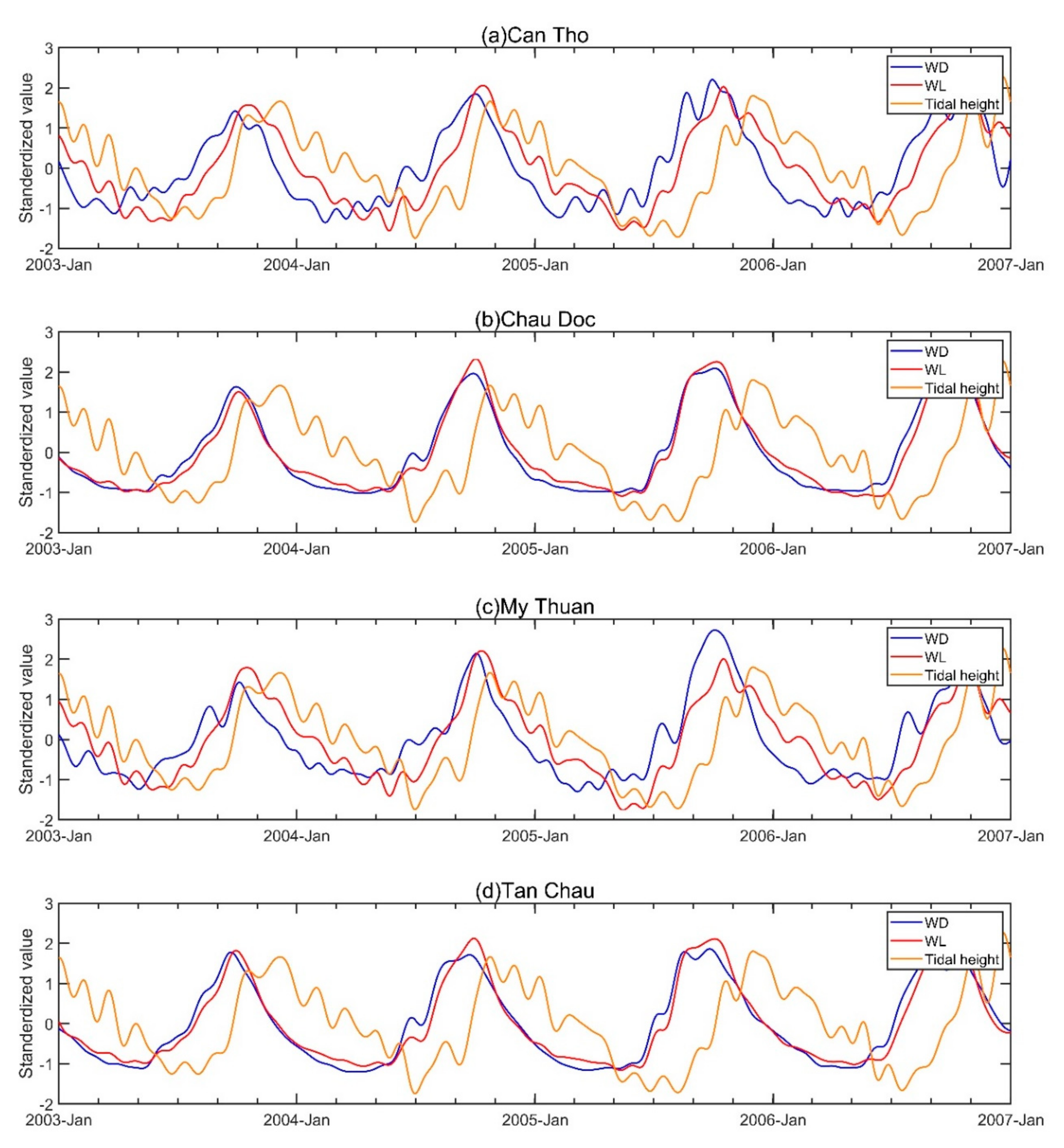
where is the average value of time series, and is the number of data in the time series. The standardized WD, WL and TH (i.e., , , and respectively) are compared for the four stations, respectively, in Figure 5.
As shown in Figure 5b,d, it is clear that the standardized WL time series are highly correlated with standardized WD time series, they reach the maximum values in early September and minimum in March and April simultaneously. Influences from ocean tide are minor, and the ocean tidal height series reaches its maximum and minimum values in different months. However, in Figure 5a,c, there exists large deviation between WD and WL time series. In the lower stations, the WL reaches its minimum and maximum value about a month later than WD, consistent with the initial phase difference of around 30° stated above (Table 4). For most cases, WL (red line) is set between WD (blue line) and TH (yellow line), emphasizing the influence of the ocean on WL. Previous studies attribute this phase difference to floods up and down or a time lag caused by tidal propagation [52]. Since this phenomenon is more apparent in stations closer to the estuaries, we speculate it is mainly caused by the mixing of fluvial-dominated and marine-dominated fluctuations at the annual and semiannual scale.
Theoretically, when two signals with the same period () are combined, the new signal will have the same period () but a different initial phase (), is expressed as:
where , , and are three different amplitudes, , , and are three initial phases, and refers to time epoch. The proof of Equation (8) is listed in Appendix A.
Since annual and semiannual signals are major components in the WL, WD, TH time series, the fluvial-dominated annual (semiannual) signal and marine-dominated annual (semiannual) signal form a mixed annual (semiannual) WL time series in the MD. For both WL and TH fluctuating in the vertical direction, the WL will be potentially corrected by annual and semiannual ocean tidal components if the TH time series are involved in the power function fitting process. This will be further explored in the next subsection. However, Equation (8) does not work for ocean tidal components shorter than half-monthly one, because of possible non-linear interaction among fluvial factors, bottom topography of an estuarine channel and ocean tidal backwater. This leads to the non-linear change of amplitude and phase during the inland propagation process.
3.2. Incorporating Long-Period Ocean Tidal Components into Rating Curve
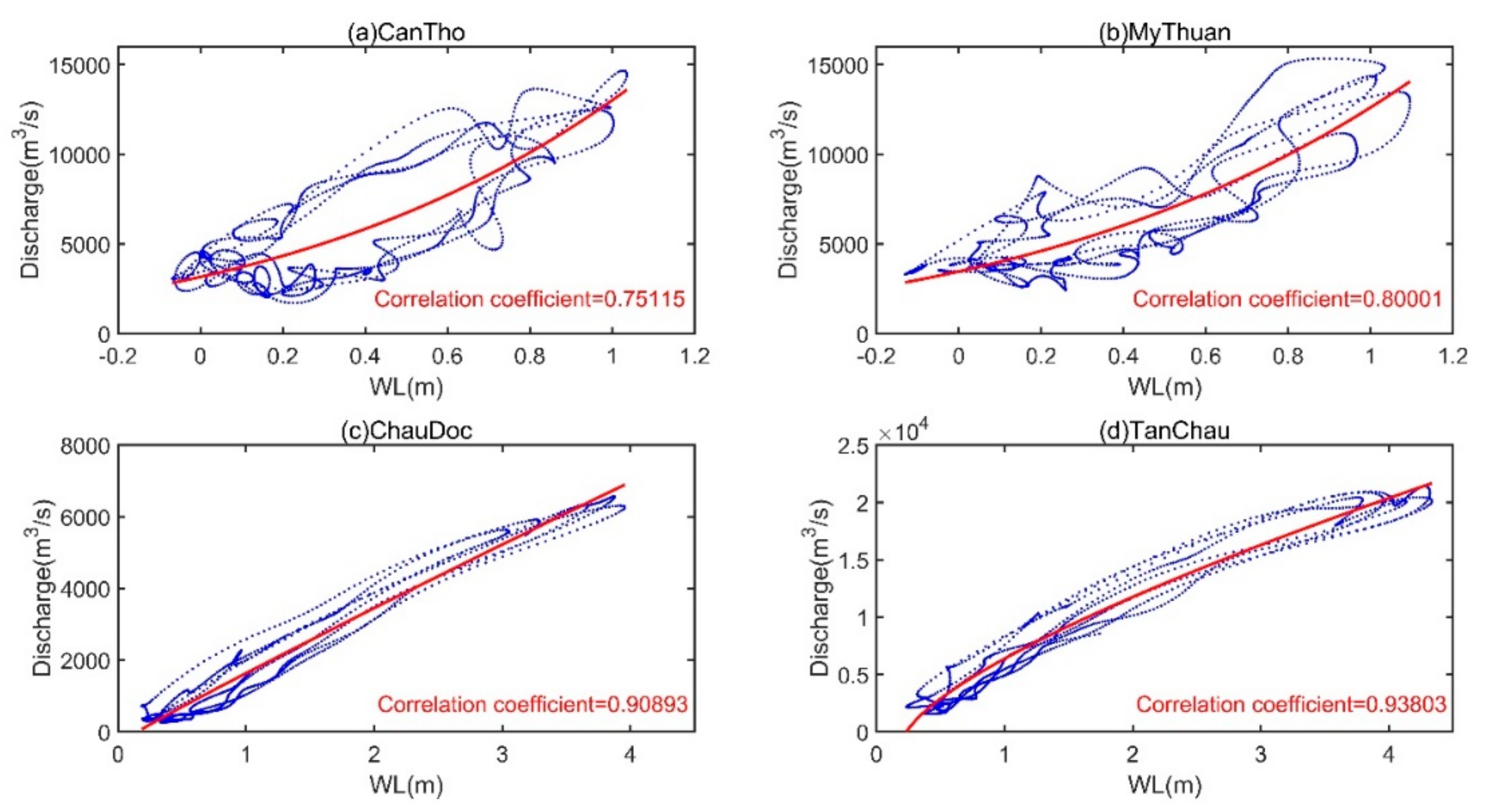
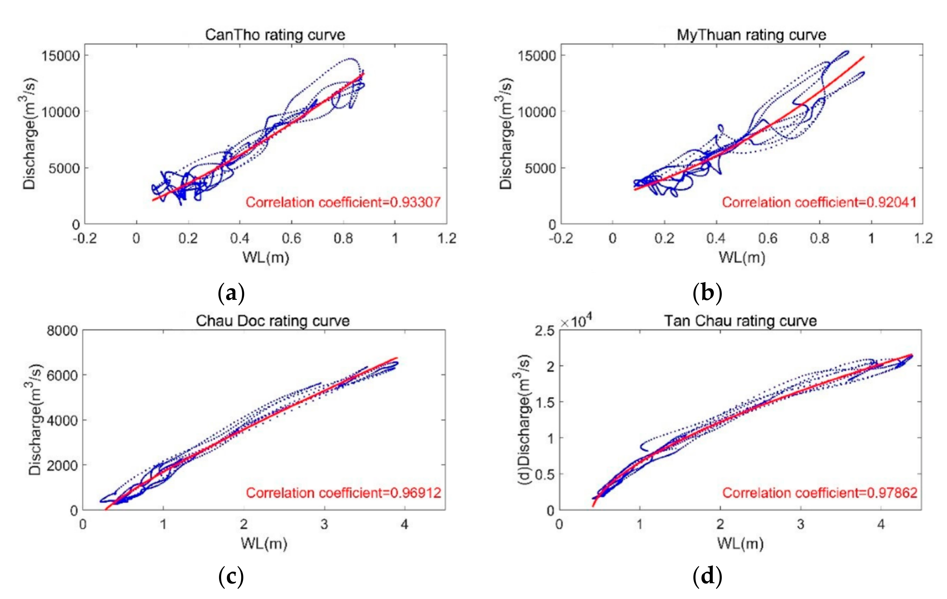
Before incorporating long-period ocean tidal components into the rating curve, short-period fluctuations in both WD and WL time series, including short-period diurnal and semidiurnal ocean tides, have to be removed. As mentioned in Section 2.1, this can be achieved by a Butterworth filter that suppresses all high-frequency signals with a period shorter than 15 days. Consistent with the filtered time series (Figure 2), the rating curve with filtered time series of WD and WL at the four stations are plotted in terms of phase diagrams (Figure 6).
Compared with those in Figure 4, it is clear that the correlation coefficients have been improved significantly (Figure 6). However, the elliptical loops are still apparent, indicating a time lag between WL and WD time series, as mentioned in Section 3.1.
Given that the relationship between , , has been analyzed in Section 3.1, it is likely that the elliptical looping phenomenon is largely due to semiannual and annual ocean tidal components. For both WL and TH fluctuating in the vertical direction, the time series were applied to separate the tide-induced fluctuation from the WL time series through a fitting process. The WL free from tide influence, , is defined as:
where, is a coefficient that rescales the . Consequently, the relationship among WD, WL, can be represented by:
where , , , and are to be determined from the observed WD, WL, and TH time series. Through a non-linear fitting [53,54], , , , and can be determined, and is obtainable.
4. Results and Discussion
The rating curves of and WD are shown (Figure 7), yielding much higher correlation coefficients when compared to the rating curves of original WD and WL time series. Although rating curves of the Can Tho and My Thuan stations still display lower correlation coefficients than their upper counterparts, significant improvement has been observed. Additionally, the elliptical looping phenomenon related to ‘time-lag’ between WL and WD is also diminished for all four selected stations. As a countercheck, the time series of WD and for the two stations close to the estuary are shown in Figure 8, revealing no apparent time lag.
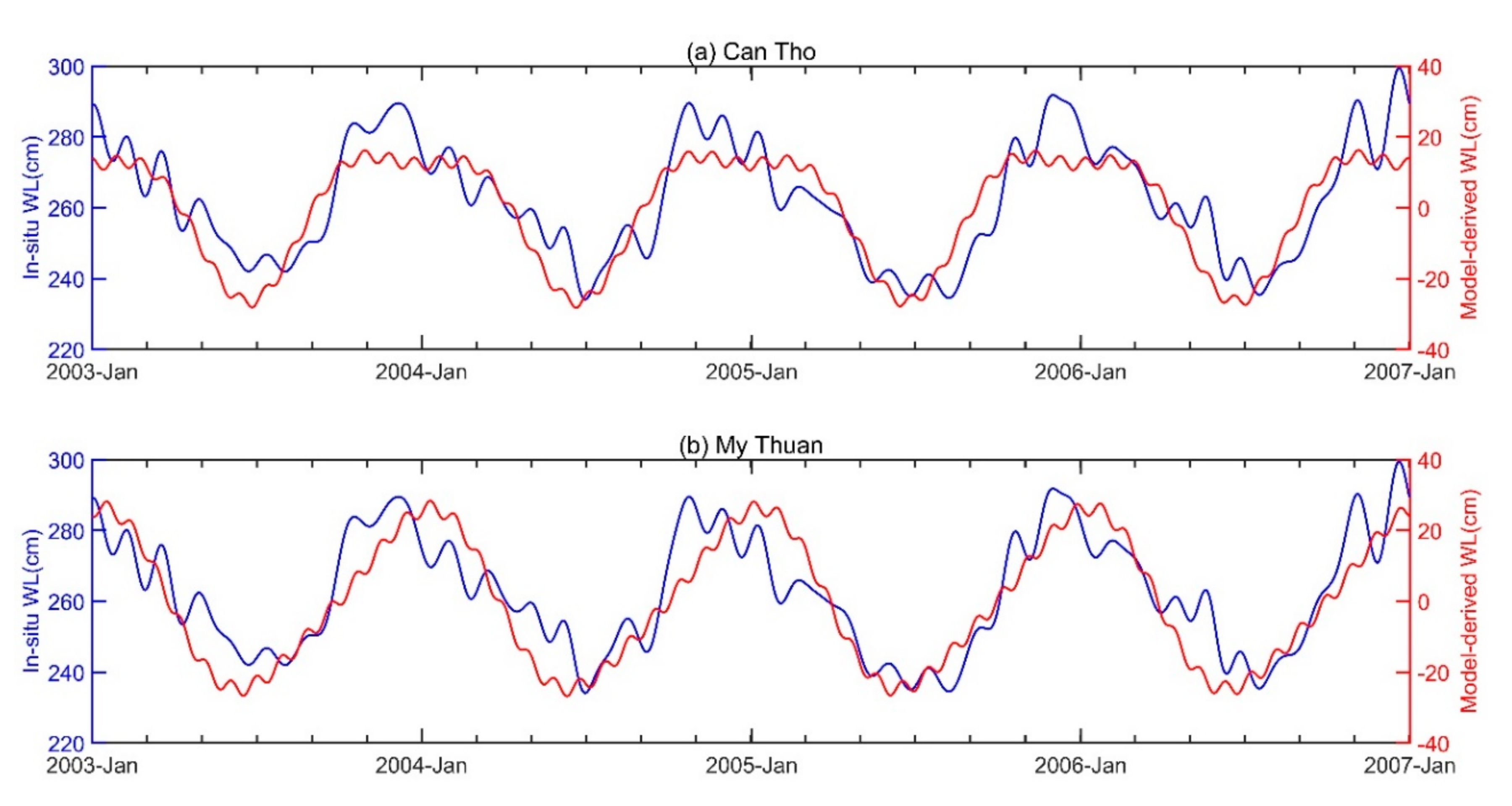
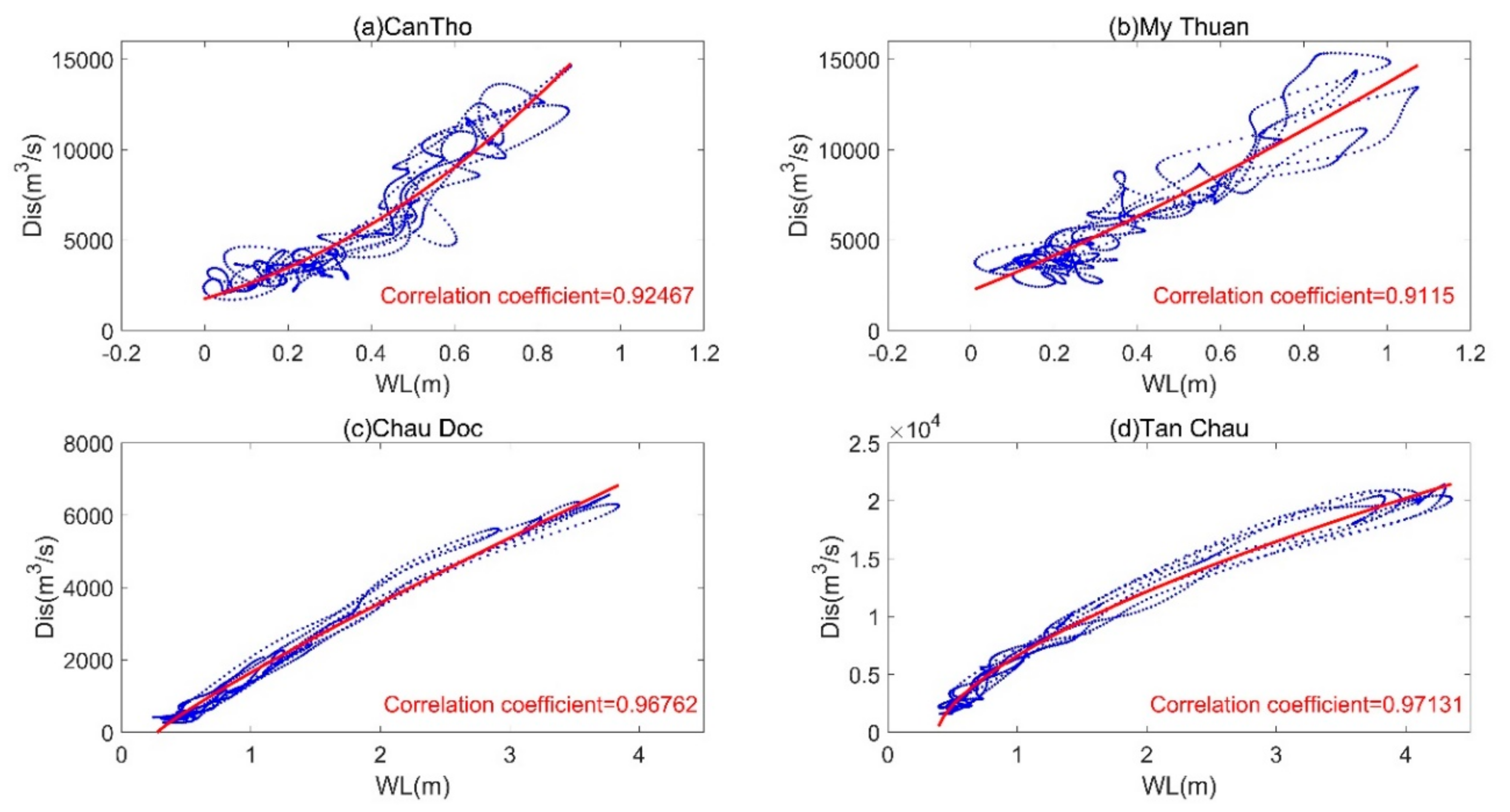
In the absence of tide gauge data, the TH time series generated from a global ocean tide model would be a viable alternative, because it can provide ocean tidal height components for the global ocean. The method for obtaining model-derived TH time series has been stated in Section 2.3. The model-derived TH series and in-situ gauged tidal height time series are displayed, manifesting high similarity with each other (Figure 9). Employing the above methodology, the rating curves of the four stations have been recovered using model-derived TH time series (Figure 10).
Although the correlation coefficients of the rating curve fitting generated by model-derived TH time series (Figure 10) are slightly lower than by in-situ tide gauge TH time series (Figure 7), the improvement is considerable when compared to the original unmodified rating curves. This is because most global ocean tide models are derived from satellite altimetry, with the model accuracies lower than that of gauge-derived TH, in particular coastal regions [39]. Given the above results, it is appropriate to use an ocean tidal model to partially recover rating curves over tide-dominated regions.
To evaluate the accuracy of the recovered rating curves, the estimated WD time series via Equation (10) generated from both model-derived and in-situ TH time series are compared with the in-situ WD during 2003–2006. Table 5 lists all determined coefficients of Equation (10) along with the assessment metrics (i.e., R-Square, PCC, NSE) that assess the estimated WD against in-situ WD. For both WD estimated based on in-situ and model-derived TH data, all the assessment metrics yield high-correlation values at all the four stations, suggesting our method can partially recover the tide-free WL for estimating WD. Overall, the recovered stage–discharge relation is capable of predicting a relatively reliable WD. These results also validate the data analysis in Section 3.
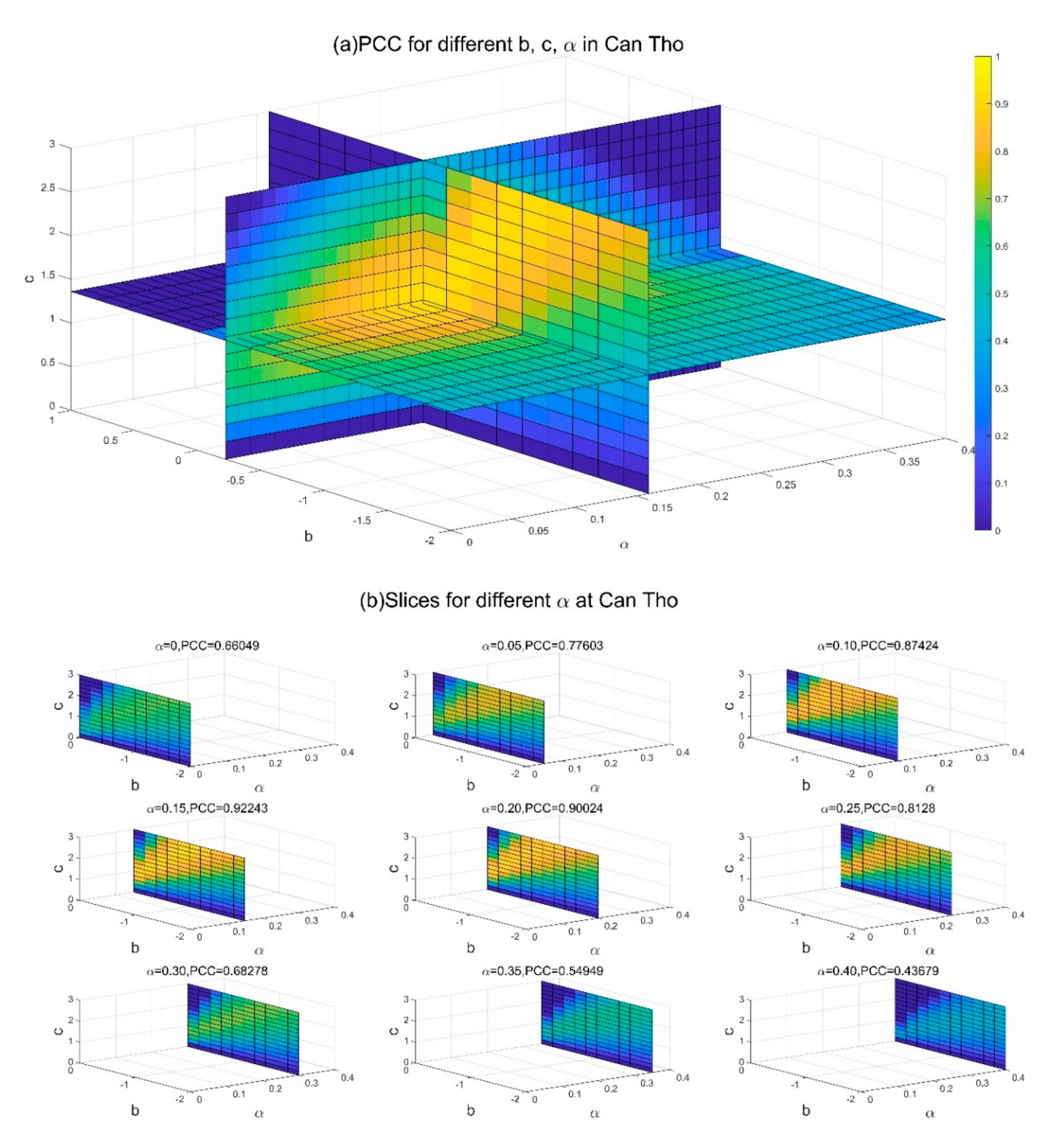
To highlight the importance of tidal separation by the term in Equation (10), the PCC values with different combinations of coefficient , , and were calculated with their best fitted fixed. Taking Can Tho station as an example (Figure 11), and impact the PCC values (i.e., > 0.9) significantly, only if is ~0.16. The same holds for My Thuan station. Therefore, adding the term to the conventional power function (i.e., Equation (5)) is necessary for the improvement of the stage–discharge relation in the MD, which is in the fluvial-to-marine transition zone. In summary, we found that an appropriate is a prerequisite for the PCC larger than 0.9.
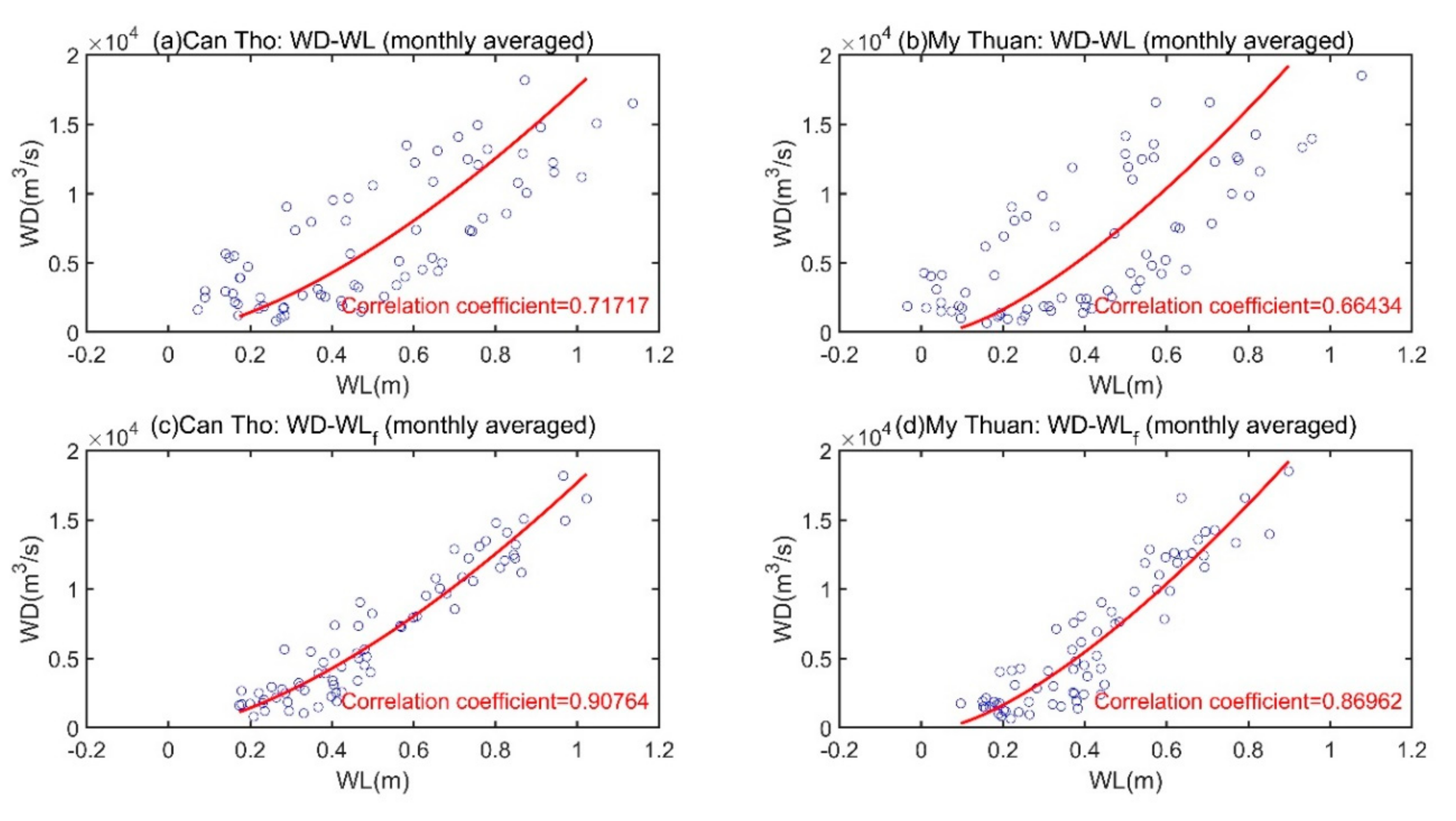
To assess the applicability of the determined coefficients of Equation (10) for Can Tho and My Thuan station time series during 2003–2006, these coefficients were directly employed for the analysis of the WL and TH data time series during 2009–2014. The predicted WD were then compared with the monthly in-situ WD (Figure 12), since only monthly WD are available for Can Tho and My Thuan stations. Hence, and were monthly averaged before the comparison. For both Can Tho and My Thuan stations, tide-free WL, , leads to higher correlation coefficients and diminishes the looping curve problem to a large degree. This indicates that coefficient appears to be stable during our study period.
Despite a substantial improvement made in this study, small deviations from the ideal power function still exist, particularly for the two stations closest to the estuary mouth. After all, the interaction between fluvial and marine processes are complicated near estuary mouths [55]. Remaining effects cannot be neglected. For instance, WD should pose a non-negligible effect on the tidal propagation along the river channel during the wet season. Overland flows inward or outward from the Tonle Sap Lake would likely be another important factor affecting the stage–discharge relations, because this lake operates as a natural reservoir that regulates Mekong river discharge from the river delta to the coastal ocean [34,56,57]. Erosion and deposition alter hydraulic geometry and increase channel bottom friction and, hence, contribute to the potential instability of the stage–discharge relation. Furthermore, numerous clusters of dams were built along the main stream of Mekong river, which may also alter the stage–discharge relation [21,22]. Sea level rise, which closely connected to salt intrusion and coastal erosion problems may alter the estuarine topography condition, resulting in a secular shift of ocean tidal components [23,26]. Agricultural practices and deforestation also provide additional impact on the evapotranspiration balance of the catchment area. Furthermore, since short-term signals were filtered out or failed to be captured by daily sampling, the short-term variations in WD and WL have not been quantitatively investigated. These considerations represent the current limitations of this study.
5. Conclusions
Instead of seeking a qualitative explanation of the stage–discharge relation influenced by the ocean tidal backwater effect, this study quantitatively analyzes the relations among water discharge (WD), water level (WL), and ocean tidal components via their standardized forms. We found that annual and semiannual ocean tidal components are significant contributors to the deviation between WL and WD time series. In particular, the annual and semiannual periods of ocean tidal backwater result in the elliptic loop associated with the presence of time lag between WL and WD.
Based on these findings, we adapt the stage–discharge relation to accommodate the effects of annual and semiannual ocean tidal components. It was found that the WD estimated from the de-tided WL yields PCC and NSE values of ~0.9. Although the de-tided WL time series generated based on the TH time series from the OSU12 global ocean tide model are slightly less accurate than that of tide gauge data, the ocean tide model is a viable alternative to partially recover the stage–discharge relation for estuaries in the absence of tide gauge stations.
Further improvement lies in identifying remaining effects contributing to the potential instability of the stage–discharge relation, which include the non-negligible effect of seasonal WD on ocean tidal propagation, the Tonle Sap lake regulation effect on the Mekong river discharge, erosion and deposition effects on the hydraulic geometry, and channel bottom friction. The impact of human activities and artificial structure in the Mekong River area, as well as its interaction with climate change, should also be highlighted. Those factors may introduce a long-term change trend into the WL–WD relationship.
The recent remotely-sensed water balance variables with improved temporal resolutions, such as 8-day MODIS evapotranspiration [58], daily TRMM precipitation [59], and daily GRACE terrestrial water storage data products [60], should enable us to compute tide-free WD, which is independent of in-situ measurements based on the water balance equation [36]. This can serve as a countercheck against the in-situ WD for assessing the first two remaining effects.
Author Contributions
Conceptualization, H.S.F.; methodology, H.P. and J.G.; software, H.P.; validation, H.S.F. and H.P.; formal analysis, H.S.F. and H.P.; investigation, H.P.; resources, H.S.F. and L.W.; data curation, H.S.F. and J.G.; writing—original draft preparation, H.P. and H.S.F.; writing—review and editing, H.S.F., H.P., L.W. and J.G.; visualization, H.P.; supervision, H.S.F.; project administration, H.S.F.; funding acquisition, H.S.F. and L.W. All authors have read and agreed to the published version of the manuscript.
Funding
This research was funded by the National Natural Science Foundation of China (NSFC) (Grant No. 41674007; 41974003; 41374010).
Acknowledgments
We acknowledge the requested water level and discharge data from the Mekong River Commission (MRC) under an agreement, which is purchased using NSFC Grant No.: 41374010.
Conflicts of Interest
The authors declare no conflict of interest.
Appendix A
The mathematic proof of Equation (8) is shown below:
For the convenience of expression, set .
Since ,,, are constant, and are also constant. Therefore, we set and . Obviously,
Notice that
Set , and . Obviously,
where . If we set ,
References
- Zhang, H. The Analysis of the Reasonable Structure of Water Conservancy Investment of Capital Construction in China by AHP Method. Water Resour. Manag. 2008, 23, 1–18. [Google Scholar] [CrossRef]
- Cloke, H.L.; Pappenberger, F. Ensemble flood forecasting: A review. J. Hydrol. 2009, 375, 613–626. [Google Scholar] [CrossRef]
- Jarihani, A.A.; Callow, J.N.; Johansen, K.; Gouweleeuw, B. Evaluation of multiple satellite altimetry data for studying inland water bodies and river floods. J. Hydrol. 2013, 505, 78–90. [Google Scholar] [CrossRef]
- Lv, M.; Lu, H.; Yang, K.; Xu, Z.; Huang, X. Assessment of Runoff Components Simulated by GLDAS against UNH–GRDC Dataset at Global and Hemispheric Scales. Water 2018, 10, 969. [Google Scholar] [CrossRef] [Green Version]
- Fread, D.L. A Dynamic Model of Stage-Discharge Relations Affected by Changing Discharge; NOAA Technical Memorandum NWS HYDRO-16; National Weather Service: Silver Spring, MD, USA, 1973. [Google Scholar]
- Fread, D.L. Computation of stage-discharge relationships affected by unsteady flow. Water Resour. Bull. 1975, 11, 213–228. [Google Scholar] [CrossRef]
- Schmidt, A.R.; Yen, B.C. Stage-discharge ratings revisited. In Hydraulic Measurements and Experimental Methods, Proceedings of the EWRI and IAHR Joint Conference, Estes Park, CO, USA, 28 July–1 August 2002; American Society of Civil Engineers: Reston, VA, USA, 2002. [Google Scholar]
- Habib, E.H.; Meselhe, E.A. Stage-Discharge Relation for Low Gradient Tidal Streams Using Data Driven Models. J. Hydraul. Eng. 2006, 132, 482–493. [Google Scholar] [CrossRef] [Green Version]
- Chau, K.W.; Wu, C.L.; Li, Y.S. Comparison of several Flood Forecasting Models in Yangtze River. J. Hydrol. Eng. 2005, 10, 485–491. [Google Scholar] [CrossRef] [Green Version]
- Jain, S.K. Modelling river stage-discharge-sediment rating relation using support vector regression. Hydrol. Res. 2012, 43, 851–861. [Google Scholar] [CrossRef]
- Jain, S.K.; Chalisgaonkar, D. Setting up stage-discharge relations using ANN. J. Hydrol. Eng. 2000, 5, 428–433. [Google Scholar] [CrossRef]
- Sudheer, K.P.; Jain, S.K. Radial basis function neural network for modeling rating curves. J. Hydrol. Eng. 2003, 8, 161–164. [Google Scholar] [CrossRef]
- Dawson, C.W.; Wilby, R.L. Hydrological modelling using artificial neural networks. Prog. Phys. Geog. 2001, 25, 80–108. [Google Scholar] [CrossRef]
- Bhattacharya, B.; Solomatine, D.P. Application of artificial neural network in stage-discharge relationship. In Proceedings of the 4th International Conference on Hydroinformatics, Iowa City, IA, USA, 23–27 August 2000. [Google Scholar]
- Simons, D.B.; Stevens, M.A.; Duke, J.H. Predicting stages on sand-bed rivers. Harb. Coast. Eng. Div. 1973, 99, 231–243. [Google Scholar]
- Dawdy, D.R. Depth-Discharge Relations of Alluvial Stream-Discontinuous Rating Curves. U.S. Geological Survey 1961; Report No. WSP 1498-C; U.S.G.P.O.: Washington, DC, USA, 1961. [Google Scholar]
- Hortle, K.G. Fisheries of the Mekong River Basin. In The Mekong Biophysical Environment of an International River Basin; Ian, C.C., Ed.; Academic Press: New York, NY, USA, 2009; pp. 197–239. [Google Scholar]
- Sassi, M.G.; Hoitink, A.J.F.; de Brye, B.; Deleersnijder, E. Downstream hydraulic geometry of a tidally influenced river delta. J. Geophys. Res. 2012, 117, F04022. [Google Scholar] [CrossRef]
- Gugliotta, M.; Saito, Y.; Nguyen, V.; Ta, T.K.O.; Nakashima, R.; Tamura, T.; Uehara, K.; Katsuki, K.; Yamamoto, S. Process regime, salinity, morphological, and sedimentary trends along the fluvial to marine transition zone of the mixed-energy Mekong River delta, Vietnam. Cont. Shelf Res. 2017, 147, 7–26. [Google Scholar] [CrossRef]
- Arias, M.E.; Cochrane, T.A.; Norton, D.; Killeen, T.J.; Khon, P. The Flood Pulse as the Underlying Driver of Vegetation in the Largest Wetland and Fishery of the Mekong Basin. AMBIO 2013, 42, 864–876. [Google Scholar] [CrossRef] [Green Version]
- Hecht, J.S.; Lacombe, G.; Arias, M.E.; Dang, T.D.; Piman, T. Hydropower dams of the Mekong River basin: A review of their hydrological impacts. J. Hydrol. 2019, 568, 285–300. [Google Scholar] [CrossRef]
- Li, X.; Liu, J.P.; Saito, Y.; Nguyen, V.L. Recent evolution of the Mekong Delta and the impacts of dams. Earth Sci. Rev. 2017, 175, 1–17. [Google Scholar] [CrossRef]
- Brunier, G.; Anthony, E.J.; Goichot, M.; Provansal, M.; Dussoillez, P. Recent morphological changes in the Mekong and Bassac river channels, Mekong delta: The marked impact of river-bed mining and implications for delta destabilization. Geomorphology 2014, 224, 177–191. [Google Scholar] [CrossRef]
- Xue, Z.; Liu, J.P.; DeMaster, D.; Van, N.L.; Ta, T.K.O. Late Holocene Evolution of the Mekong Subaqueous Delta. Mar. Geol. 2010, 269, 46–60. [Google Scholar] [CrossRef]
- Paul, A.C. The Geology of the Lower Mekong River. In The Mekong Biophysical Environment of an International River Basin; Ian, C.C., Ed.; Academic Press: New York, NY, USA, 2009; pp. 13–28. [Google Scholar]
- Dang, T.D.; Cochrane, T.A.; Arias, M.E. Future hydrological alterations in the Mekong Delta under the impact of water resources development, land subsidence and sea level rise. J. Hydrol. Reg. Stud. 2018, 15, 119–133. [Google Scholar] [CrossRef]
- Gugliotta, M.; Saito, Y.; Nguyen, V.L.; Ta, T.K.O.; Tamura, T. Sediment distribution and depositional processes along the fluvial to marine transition zone of the Mekong River delta, Vietnam. Sedimentology 2019, 66, 146–164. [Google Scholar]
- Hoa, L.T.V.; Nhan, N.H.; Wolanski, E.; Cong, T.T.; Shigeko, H. The combined impact on the flooding in Vietnam’s Mekong River delta of local man-made structures, sea level rise, and dams upstream in the river catchment. Estuar. Coast. Shelf Sci. 2007, 71, 110–116. [Google Scholar]
- Woodruff, J.D.; Irish, J.L.; Camargo, S.J. Costal flooding by tropical cyclones and sea-level rise. Nature 2013, 504, 44–52. [Google Scholar] [CrossRef] [Green Version]
- Werner, A.D.; Bakker, M.; Post, V.E.A.; Vandenbohede, A.; Lu, C.; Ataie-Ashtiani, B.; Barry, D.A. Seawater intrusion processes, investigation and management: Recent advances and future challenges. Adv. Water Resour. 2013, 51, 3–26. [Google Scholar] [CrossRef]
- Minderhoud, P.S.J.; Coumou, L.; Erkens, G.; Middelkoop, H.; Stouthamer, E. Mekong delta much lower than previously assumed in sea-level rise impact assessments. Nature Comm. 2019, 10, 1–13. [Google Scholar]
- Wassmann, R.; Nguyen, X.H.; Chu, T.H.; To, P.T. Sea level rise affecting the Vietnamese Mekong Delta: Water elevation in the flood season and implications for rice production. Clim. Chang. 2004, 66, 89–107. [Google Scholar] [CrossRef]
- Kummu, M.; Tes, S.; Yin, S.; Adamson, P.; Józsa, J.; Koponen, J.; Richey, J.; Sarkkula, J. Water balance analysis for the Tonle Sap Lake–floodplain system. Hydrol. Process. 2014, 28, 1722–1733. [Google Scholar] [CrossRef]
- Tangdamrongsub, N.; Ditmar, P.G.; Steele-Dunne, S.C.; Gunter, B.C.; Sutanudjaja, E.H. Assessing total water storage and identifying flood events over Tonlé Sap basin in Cambodia using GRACE and MODIS satellite observations combined with hydrological models. Remote Sens. Environ. 2016, 181, 162–173. [Google Scholar] [CrossRef] [Green Version]
- Frappart, F.; Biancamaria, S.; Normandin, C.; Blarel, F.; Bourrel, L.; Aumont, M.; Azemar, P.; Vu, P.L.; Le Toan, T.; Lubac, B.; et al. Influence of recent climatic events on the surface water storage of the Tonle Sap Lake. Sci. Total Environ. 2018, 636, 1520–1533. [Google Scholar] [CrossRef] [Green Version]
- Zhou, L.H.; Fok, H.S.; Ma, Z.T.; Chen, Q. Upstream Remotely-Sensed Hydrological Variables and Their Standardization for Surface Runoff Reconstruction and Estimation of the Entire Mekong River Basin. Remote Sens. 2019, 11, 1064. [Google Scholar]
- El-Jabi, N.; Wakin, G.; Sarraf, S. Stage-Discharge Relationship in Tidal Rivers. Ocean Eng. 1992, 118, 166–174. [Google Scholar] [CrossRef]
- Tozer, B.; Sandwell, D.T.; Smith, W.H.F.; Olson, C.; Beale, J.R.; Wessel, P. Global bathymetry and topography at 15 arc seconds: SRTM15+. Earth Space Sci. 2019, 1847–1864. [Google Scholar] [CrossRef]
- Koehnken, L. IKMP Discharge and Sediment Monitoring Program Review, Recommendations and Data Analysis. Part 1 and 2. Tech. Advice Water 2012, 2–36. [Google Scholar]
- Merrifield, M.; Aarup, T.; Allen, A.; Aman, B.; Caldwel, P.; Fernandes, R.; Hayashibara, H.; Hernandez, F.; Kilonsky, B.; Martin Miguez, B.; et al. The Global Sea Level Observing System (GLOSS). In Proceedings of the Ocean Obs. 09, Ocean information for Society: Sustaining the Benefits, Realizing the Potential, Venice–Lido, Italy, 21–25 September 2009. [Google Scholar]
- Godin, G. The daily mean level and short period seiches. IHR 1966, 43, 75–89. [Google Scholar]
- Godin, G. The Propagation of Tides up Rivers with Special Considerations on the Upper Saint Lawrence River. Estuarine Coas. Shelf Sci. 1999, 48, 307–324. [Google Scholar] [CrossRef]
- Godin, G. The Analysis of Tides; University of Toronto Press: Toronto, ON, Canada; Liverpool University Press: Buffalo, NY, USA, 1972. [Google Scholar]
- Brooks, B.A.; Merrifield, M.A.; Foster, J.; Werner, C.L.; Gomez, F.; Bevis, M.; Gill, S. Space geodetic determination of spatial variability in relative sea level change. Geophys. Res. Lett. 2007, 34, L01611. [Google Scholar] [CrossRef] [Green Version]
- Stammer, D.; Ray, R.D.; Andersen, O.B.; Arbic, B.K.; Bosch, W.; Carrère, L.; Cheng, Y.; Chin, D.S.; Dushaw, B.D.; Egbert, G.D.; et al. Accuracy assessment of global barotropic ocean tide models. Rev. Geophys. 2014, 52, 243–282. [Google Scholar] [CrossRef] [Green Version]
- Fok, H.S.; Iz, H.B.; Shum, C.K.; Yi, Y.; Andersen, O.; Braun, A.; Chao, Y.; Han, G.; Kuo, C.Y.; Matsumoto, K.; et al. Evaluation of Ocean Tide Models Used for Jason-2 Altimetry Corrections. Mar. Geod. 2010, 33 (Suppl. S1), 285–303. [Google Scholar] [CrossRef] [Green Version]
- Fok, H.S. Ocean Tides Modeling Using Satellite Altimetry. Ph.D. Thesis, School of Earth Sciences, State University, Columbus, OH, USA, 2012. [Google Scholar]
- Gupta, H.V.; Kling, H.; Yilmaz, K.K.; Martinez, G.F. Decomposition of the mean squared error and NSE performance criteria: Implications for improving hydrological modelling. J. Hydrol. 2009, 377, 80–91. [Google Scholar] [CrossRef] [Green Version]
- Mansanarez, V.; Renard, B.; Coz, J.L.; Lang, M.; Darienzo, M. Shift Happens! Adjusting stage-discharge rating curves to morphological changes at known times. Water Resour. Res. 2019, 55, 2876–2899. [Google Scholar] [CrossRef]
- Guo, L.C.; Zhu, C.Y.; Wu, X.; Wan, Y.; Jay, D.A.; Townend, I.; Wang, Z.B.; He, Q. Strong Inland Propagation of Low-Frequency Long Waves in River Estuaries. Geophys. Res. Lett. 2020. [Google Scholar] [CrossRef]
- Jay, D.A. Green’s Law Revisited: Tidal Long-Wave Propagation in Channels With Strong Topography. J. Geophys. Res. 1991, 96, 586–598. [Google Scholar] [CrossRef]
- Miller, J.L.; Gardner, L.R. Sheet flow in a salt-marsh basin, North Inlet, South Carolina. Estuaries 1981, 4, 234–237. [Google Scholar] [CrossRef]
- Gavin, H.P. The Levenberg-Marquardt Method for Non-Linear Least Squares Curve-Fitting Problems. Department of Civil and Environmental Engineering, Duke University: Durham, NC, USA, 2013; pp. 1–17. [Google Scholar]
- Seber, G.A.F.; Wild, C.J. Non-Linear Regression; Wiley-Interscience: Hoboken, NJ, USA, 2003. [Google Scholar]
- Möller, I.; Kudella, M.; Rupprecht, F.; Spencer, T.; Paul, M.; van Wesenbeeck, B.K.; Wolters, G.; Jensen, K.; Bouma, T.J.; Miranda-Lange, M.; et al. Wave attenuation over coastal salt marshes under storm surge conditions. Nature Geosci. 2014, 7, 727–731. [Google Scholar] [CrossRef] [Green Version]
- Arias, M.E. Impacts of Hydrological Alterations in the Mekong Basin to Tonle Sap Ecosystem. Ph.D. Thesis, Department of Civil and Natural Resources Engineering, University of Canterbury, Christchurch, New Zealand, 2003. [Google Scholar]
- Cochrane, T.A.; Arias, M.E.; Piman, T. Historical impact of water infrastructure on water levels of the Mekong River and Tonle Sap system. Hydrol. Earth Syst. Sc. 2014, 18, 4529–4541. [Google Scholar] [CrossRef] [Green Version]
- Running, S.; Mu, Q.; Zhao, M. MYD16A2 MODIS/Aqua Net Evapotranspiration 8-Day L4 Global 500m SIN Grid V006 [Data Set]. NASA EOSDIS Land Processes DAAC. 2017. Available online: https://lpdaac.usgs.gov/products/myd16a2v006/ (accessed on 25 October 2020).
- Huffman, G.J.; Bolvin, D.T. Real-Time TRMM Multi-Satellite Precipitation Analysis Data Set Documentation; NASA Goddard Space Flight Center location: Greenbelt, MD, USA; Science Systems and Applications, Inc.: Hampton, VA, USA, 2015. [Google Scholar]
- Gouweleeuw, B.T.; Kvas, A.; Gruber, C.; Gain, A.K.; Mayer-Gürr, T.; Flechtner, F.; Güntner, A. Daily GRACE gravity field solutions track major flood events in the Ganges–Brahmaputra Delta. Hydrol. Earth Syst. Sc. 2018, 22, 2867–2880. [Google Scholar] [CrossRef] [Green Version]
Figure 1.
Map of Mekong Delta (MD), with two pairs of hydrological gauge stations (i.e., Can Tho and Chau Doc, and My Thuan and Tan Chau) situated near the estuaries. (The topography dataset, called earth_relief_30s, is a derived product of SRTM15+ [38], which is obtainable from http://mirrors.ustc.edu.cn/gmt/data/).

Figure 2.
Low-pass filtered (blue) and original (blue dash) time series of water discharge and water level (red) over (a) Can Tho, (b) My Thuan, (c) Chau Doc, and (d) Tan Chau stations, respectively, and (e) time series of ocean tidal height (sea level) at Vung Tau station spanning from January 2003 to December 2006.

Figure 3.
Spectra of the (a) hourly and (b) daily averaged ocean tidal height time series in Vung Tau tide gauge station.
Figure 3.
Spectra of the (a) hourly and (b) daily averaged ocean tidal height time series in Vung Tau tide gauge station.

Figure 4.
(a–d) Relationship between water level (WL) and water discharge (WD) (original daily sampled time series) for the four selected hydrological stations in Mekong Delta.
Figure 4.
(a–d) Relationship between water level (WL) and water discharge (WD) (original daily sampled time series) for the four selected hydrological stations in Mekong Delta.

Figure 5.
Comparison of standardized WD, WL, and tidal height time series in (a) Can Tho, (b) Chau Doc, (c) My Thuan, and (d) Tan Chau station, respectively.
Figure 5.
Comparison of standardized WD, WL, and tidal height time series in (a) Can Tho, (b) Chau Doc, (c) My Thuan, and (d) Tan Chau station, respectively.

Figure 6.
(a–d) Relationship between WL and WD (low pass filtered time series) for the selected four hydrological stations in the Mekong Delta.
Figure 6.
(a–d) Relationship between WL and WD (low pass filtered time series) for the selected four hydrological stations in the Mekong Delta.

Figure 7.
(a–d) Relationship between and WD (low pass filtered time series) for the selected four hydrological stations in the Mekong Delta.
Figure 7.
(a–d) Relationship between and WD (low pass filtered time series) for the selected four hydrological stations in the Mekong Delta.

Figure 8.
WD and tide-free WL time series from 2003 to 2006 in (a) Can Tho and (b) My Thuan stations.
Figure 8.
WD and tide-free WL time series from 2003 to 2006 in (a) Can Tho and (b) My Thuan stations.

Figure 9.
The comparison between OSU12 model-derived WL and in-situ WL at (a) Can Tho and (b) My Thuan during 2003–2006.
Figure 9.
The comparison between OSU12 model-derived WL and in-situ WL at (a) Can Tho and (b) My Thuan during 2003–2006.

Figure 10.
Recovered rating curves at (a) Can Tho, (b) My Thuan, (c) Chau Doc, and (d) Tan Chau stations using model-derived ocean tidal height as input.
Figure 10.
Recovered rating curves at (a) Can Tho, (b) My Thuan, (c) Chau Doc, and (d) Tan Chau stations using model-derived ocean tidal height as input.

Figure 11.
(a) Different PCC (presented in color bar) for different ,
and
using time series from Can Tho station, and (b) slices of (a) for nine chosen α, with maximum PCC for each α shown from the above subplots.
Figure 11.
(a) Different PCC (presented in color bar) for different ,
and
using time series from Can Tho station, and (b) slices of (a) for nine chosen α, with maximum PCC for each α shown from the above subplots.

Figure 12.
(a,b) Stage discharge relation from original WL, and (c,d) tide-free WL for Can Tho and My Thuan stations.
Figure 12.
(a,b) Stage discharge relation from original WL, and (c,d) tide-free WL for Can Tho and My Thuan stations.


Table 1.
The datasets used in this study.
| Products | Location | Time Span | Temporal Resolution |
|---|---|---|---|
| In Situ Stations’ Water Level Data | Can Tho | 2003–2006 2009–2014 | Daily average |
| My Thuan | 2003–2006 2009–2014 | ||
| Chau Doc | 2003–2006 | ||
| Tan Chau | 2003–2006 | ||
| In Situ Stations’ Discharge Data | Can Tho | 2003–2006 2009–2014 | Daily (before 2006) Monthly (after 2009) |
| My Thuan | 2003–2006 2009–2014 | ||
| Chau Doc | 2003–2006 | ||
| Tan Chau | 2003–2006 | ||
| Tidal Gauge Data | Vung Tau | 2003–2014 | Hourly |
| OSU12 Global Ocean Tide Model Data | 9.375N, 106.375E | Tidal constituents (Sa, Ssa, Mm) | |
| 10.125N, 107.125E |
Table 2.
Maximum, minimum, mean values, and standard deviations of original and processed time series.
Table 2.
Maximum, minimum, mean values, and standard deviations of original and processed time series.
| Variable | Station | Maximum | Minimum | Mean | Standard Deviation |
|---|---|---|---|---|---|
| Original Water Discharge (1 × 10⁴ m3/s) | My Thuan | 1.6500 | 0.0029 | 0.7263 | 0.4036 |
| Can Tho | 1.8400 | 0.0025 | 0.7206 | 0.4416 | |
| Tan Chau | 2.2597 | 0.1190 | 0.9359 | 0.6490 | |
| Chau Doc | 0.7120 | 0.0045 | 0.2625 | 0.2059 | |
| Processed Water Discharge (1 × 10⁴ m3/s) | My Thuan | 1.5345 | 0.2423 | 0.7262 | 0.3109 |
| Can Tho | 1.4666 | 0.1704 | 0.7209 | 0.3236 | |
| Tan Chau | 2.1400 | 0.1600 | 0.9360 | 0.6470 | |
| Chau Doc | 0.7121 | 0.0266 | 0.2626 | 0.2043 | |
| Original Water Level (m) | My Thuan | 1.4225 | −0.3355 | 0.4619 | 0.3522 |
| Can Tho | 1.4591 | −0.2707 | 0.4168 | 0.3231 | |
| Tan Chau | 4.3831 | 0.0222 | 1.6820 | 1.2544 | |
| Chau Doc | 4.0036 | −0.1486 | 1.5017 | 1.1443 | |
| Processed Water Level (m) | My Thuan | 1.2165 | −0.1304 | 0.4620 | 0.3267 |
| Can Tho | 1.0358 | −0.0685 | 0.4171 | 0.2976 | |
| Tan Chau | 4.3361 | 0.2326 | 1.6825 | 1.2498 | |
| Chau Doc | 3.9558 | 0.1863 | 1.5019 | 1.1396 | |
| Original Tide height (m) | Vung Tau | 4.3300 | −0.4400 | 2.6433 | 0.8566 |
| Processed Tide height (m) | Vung Tau | 2.9984 | 2.3413 | 2.6436 | 0.1648 |
Table 3.
Long-period ocean tidal components at two gridded locations close to Mekong and Bassac river estuaries solved at the initial time epoch of 0:00 AM, 1 January 2002 (UTC +0).
Table 3.
Long-period ocean tidal components at two gridded locations close to Mekong and Bassac river estuaries solved at the initial time epoch of 0:00 AM, 1 January 2002 (UTC +0).
| Tide Components | Point1 (9.35°N,106.375°E) (in cm) | Point2 (10.125°N, 107.125°E) (in cm) | |
|---|---|---|---|
| Sa (365.25 days) | H1 | 24.41570 | 19.06151 |
| H2 | −1.56798 | −3.91959 | |
| Ssa (182.62 days) | H1 | 1.36968 | −6.76170 |
| H2 | 3.52620 | 2.07534 | |
| Mm (27.55 days) | H1 | 1.30950 | 0.32715 |
| H2 | −1.63984 | 1.72923 | |
Table 4.
Relative power and initial phases of the three periodic signals in WD and WL time series at the four selected stations with initial phase domain defined between 0° and 360°.
Table 4.
Relative power and initial phases of the three periodic signals in WD and WL time series at the four selected stations with initial phase domain defined between 0° and 360°.
| Station | Period: 365 Days | Period: 182.5 Days | Period: 14.7475 Days | ||||
|---|---|---|---|---|---|---|---|
| Relative Power | Initial Phase | Relative Power | Initial Phase | Relative Power | Initial Phase | ||
| Can Tho | WD | 1 | 95.2311° | 0.3060 | 173.5607° | 0.4727 | 25.1628° |
| WL | 1 | 58.5725° | 0.2535 | 168.3582° | 0.2997 | 244.1391° | |
| My Thuan | WD | 1 | 87.1219° | 0.3093 | 170.8565° | 0.5671 | 25.8326° |
| WL | 1 | 55.0654° | 0.2664 | 175.4839° | 0.3152 | 244.2108° | |
| Chau Doc | WD | 1 | 93.8689° | 0.3392 | 196.6511° | 0.0324 | 111.2065° |
| WL | 1 | 84.7393° | 0.3963 | 193.8528° | 0.0414 | 274.7407° | |
| Tan Chau | WD | 1 | 97.4019° | 0.2385 | 222.2999° | 0.0046 | 99.6860° |
| WL | 1 | 90.3988° | 0.3705 | 202.5387° | 0.0336 | 260.8400° | |
Table 5.
Assessment of the estimated WD and stage–discharge relation coefficients.
| Tidal Height Data | Station | a | b | c | R-Square | PCC | NSE | |
|---|---|---|---|---|---|---|---|---|
| In-situ measured | Can Tho | −0.2230 | 1.3661 | 0.1619 | 0.9291 | 0.9626 | 0.9266 | |
| My Thuan | −0.8665 | 2.4063 | 0.1480 | 0.8974 | 0.9468 | 0.8964 | ||
| Chau Doc | 0.2756 | 0.8592 | 0.1577 | 0.9790 | 0.9922 | 0.9843 | ||
| Tan Chau | 0.4052 | 0.6229 | 0.1819 | 0.9809 | 0.9946 | 0.9891 | ||
| OSU12 | Can Tho | −0.5949 | 2.3417 | 0.1722 | 0.8871 | 0.9383 | 0.8804 | |
| My Thuan | −0.3079 | 1.2619 | 0.1520 | 0.8631 | 0.9285 | 0.8621 | ||
| Chau Doc | 0.2762 | 0.8911 | 0.1582 | 0.9828 | 0.9934 | 0.9868 | ||
| Tan Chau | 0.3809 | 0.6335 | 0.1314 | 0.9750 | 0.9910 | 0.9820 |
Publisher’s Note: MDPI stays neutral with regard to jurisdictional claims in published maps and institutional affiliations. |
© 2020 by the authors. Licensee MDPI, Basel, Switzerland. This article is an open access article distributed under the terms and conditions of the Creative Commons Attribution (CC BY) license (http://creativecommons.org/licenses/by/4.0/).
Share and Cite
MDPI and ACS Style
Peng, H.; Fok, H.S.; Gong, J.; Wang, L. Improving Stage–Discharge Relation in The Mekong River Estuary by Remotely Sensed Long-Period Ocean Tides. Remote Sens. 2020, 12, 3648. https://0-doi-org.brum.beds.ac.uk/10.3390/rs12213648
AMA Style
Peng H, Fok HS, Gong J, Wang L. Improving Stage–Discharge Relation in The Mekong River Estuary by Remotely Sensed Long-Period Ocean Tides. Remote Sensing. 2020; 12(21):3648. https://0-doi-org.brum.beds.ac.uk/10.3390/rs12213648
Chicago/Turabian StylePeng, Hongrui, Hok Sum Fok, Junyi Gong, and Lei Wang. 2020. "Improving Stage–Discharge Relation in The Mekong River Estuary by Remotely Sensed Long-Period Ocean Tides" Remote Sensing 12, no. 21: 3648. https://0-doi-org.brum.beds.ac.uk/10.3390/rs12213648
Note that from the first issue of 2016, this journal uses article numbers instead of page numbers. See further details here.