Sea Surface Temperature and High Water Temperature Occurrence Prediction Using a Long Short-Term Memory Model

1
School of Ocean Science and Technology, Korea Maritime and Ocean University, Busan 49112, Korea
2
Korea Ocean Satellite Center, Korea Institute of Ocean Science & Technology, Busan 49112, Korea
3
Applied Ocean Science, University of Science & Technology, Daejeon 34113, Korea
*
Author to whom correspondence should be addressed.
Remote Sens. 2020, 12(21), 3654; https://0-doi-org.brum.beds.ac.uk/10.3390/rs12213654
Submission received: 12 October 2020
/
Revised: 4 November 2020
/
Accepted: 4 November 2020
/
Published: 7 November 2020
(This article belongs to the Special Issue Advances in Retrieval, Operationalization, Monitoring and Application of Sea Surface Temperature)
Abstract
:Recent global warming has been accompanied by high water temperatures (HWTs) in coastal areas of Korea, resulting in huge economic losses in the marine fishery industry due to disease outbreaks in aquaculture. To mitigate these losses, it is necessary to predict such outbreaks to prevent or respond to them as early as possible. In the present study, we propose an HWT prediction method that applies sea surface temperatures (SSTs) and deep-learning technology in a long short-term memory (LSTM) model based on a recurrent neural network (RNN). The LSTM model is used to predict time series data for the target areas, including the coastal area from Goheung to Yeosu, Jeollanam-do, Korea, which has experienced frequent HWT occurrences in recent years. To evaluate the performance of the SST prediction model, we compared and analyzed the results of an existing SST prediction model for the SST data, and additional external meteorological data. The proposed model outperformed the existing model in predicting SSTs and HWTs. Although the performance of the proposed model decreased as the prediction interval increased, it consistently showed better performance than the European Center for Medium-Range Weather Forecast (ECMWF) prediction model. Therefore, the method proposed in this study may be applied to prevent future damage to the aquaculture industry.
1. Introduction
Due to global warming, high water temperatures (HWTs) are frequently observed along the coast of the Korean Peninsula. This phenomenon has led to mass mortality of farmed fish, resulting in massive economic losses to fishermen. The HWT warning period lasted for a total of 32 days in 2017, but persisted for 43 days in 2018. If this trend continues, the damage resulting from HWTs will likely be further exacerbated. To prevent and mitigate exposure risk, it is necessary to predict HWT occurrence accurately in advance. Therefore, in this study, we present a recurrent neural network (RNN)-based long short-term memory (LSTM) model based on deep-learning technology [1,2], to predict sea surface temperatures (SSTs).
Generally, extreme MHW is defined as the top 10% of all SST values observed over the past 30 years for a particular body of water [3,4]. However, in this study, we define HWTs in the context of typical water temperatures in Korea. We follow the criteria defined by the Korean Ministry of Maritime Affairs and Fisheries, which operates a HWT alert system to prevent damage to the aquaculture sector and respond as needed to these events. The HWT alert system consists of the following three stages: level of interest, which occurs 7 days prior to onset of the temperature increase; level of watch, when the water temperature reaches 28 °C; and level of warning, when the water temperature exceeds 28 °C and lasts for 3 or more days. Since the Korea Ministry of Maritime Affairs evaluates HWT based on a threshold of 28 °C, we defined HWT as > 28 °C. In this study, the area selected for HWT prediction was the coastal region extending from Goheung to Yeosu, Jeollanam-do, Korea. This region has a high concentration of fish farms. Thus, persistent HWTs cause serious damage to the local fishing industry, as observed in the 2018 disaster, which involved the loss of 54.1 million fish/shellfish in Jeollanam-do, with a total property damage of USD 38 million [5].
In this study, we used the ERA5 product reanalysis SST data provided by the European Center for Medium-Range Weather Forecast (ECMWF) because the reliability and continuity of input data are important for training LSTM deep-learning models. The ECMWF creates numerical weather forecasts, monitors the dynamics of Earth/planetary systems that affect the weather, and provides researchers with stored weather data to improve forecasting technology [6,7].
Recently, studies on SST prediction have been actively conducted. SST prediction methods can be classified into two categories: numerical methods and data-centric methods. Some of the earlier numerical methods for SST prediction combine physical, chemical, and biological parameters and the complex interactions among them. A representative example of a mathematical model is the fully compressible, non-integer Advanced Research Weather Research and Forecasting model [8,9], developed by the University Corporation for Atmospheric Research/National Center for Atmospheric Research [10,11]. In recent studies, the performance of the physical model NEMO-Nordic in the North and Baltic seas was improved by assimilating high-resolution SST data for the model [12,13]. In contrast, data-based methods produce SST predictions from a data-centric perspective. Data-driven methods require less knowledge of the oceans and atmosphere but require large amounts of data. Methods in this category include statistical schemes such as the Markov model [14,15,16], machine learning, and artificial intelligence methods. Support vector machine [17,18] and RNNs are widely used machine-learning methods for SST prediction [19,20,21].
Although the RNN algorithm specializes in processing time-series data, long-term dependency problems arise because SST and HWT predictions require significant amounts of data from the past. The LSTM model is widely used to solve these long-term dependency problems [22,23,24,25]. The LSTM model consists of cells with multiple gates attached. The gates are divided into three types: forget, input, and output. Here, the long-term dependency problem is resolved via the forget gate. LSMT is suitable for training data based on its high correlation with previously inputted data, which has made it useful for linguistics applications [26]. LSMT has also been applied to predict concentrations of air pollutants based on traffic volume, air pollution, and meteorological time series data [27]. In the present study, we applied an LSTM model to predict SSTs and HWTs in the coastal area spanning from Goheung to Yeosu, Jeollanam-do, Korea.
In previous studies, SSTs have been predicted near the Bohia Sea in China using LSTM [28] and near the East China Sea using temporal dependence-based LSTM (TD-LSTM) [29] using large datasets of past SST observations; SST prediction is rarely achieved using other types of meteorological data in active research. Therefore, in this study, we proposed an LSTM model that uses other meteorological data to improve SST prediction performance.
This paper is organized as follows. In Section 2, we explain SST data acquisition and describe the coastal region around the Korean Peninsula selected for HWT prediction. Section 3 discusses the LSTM training methodology and SST prediction concept, and the indicators used to evaluate SST and HWT prediction performance. In Section 4 and Section 5, we describe experiments conducted using common methods and the proposed method, and their performance is compared and analyzed. Section 6 provides our conclusions.
2. Study Area and Data
2.1. Study Area
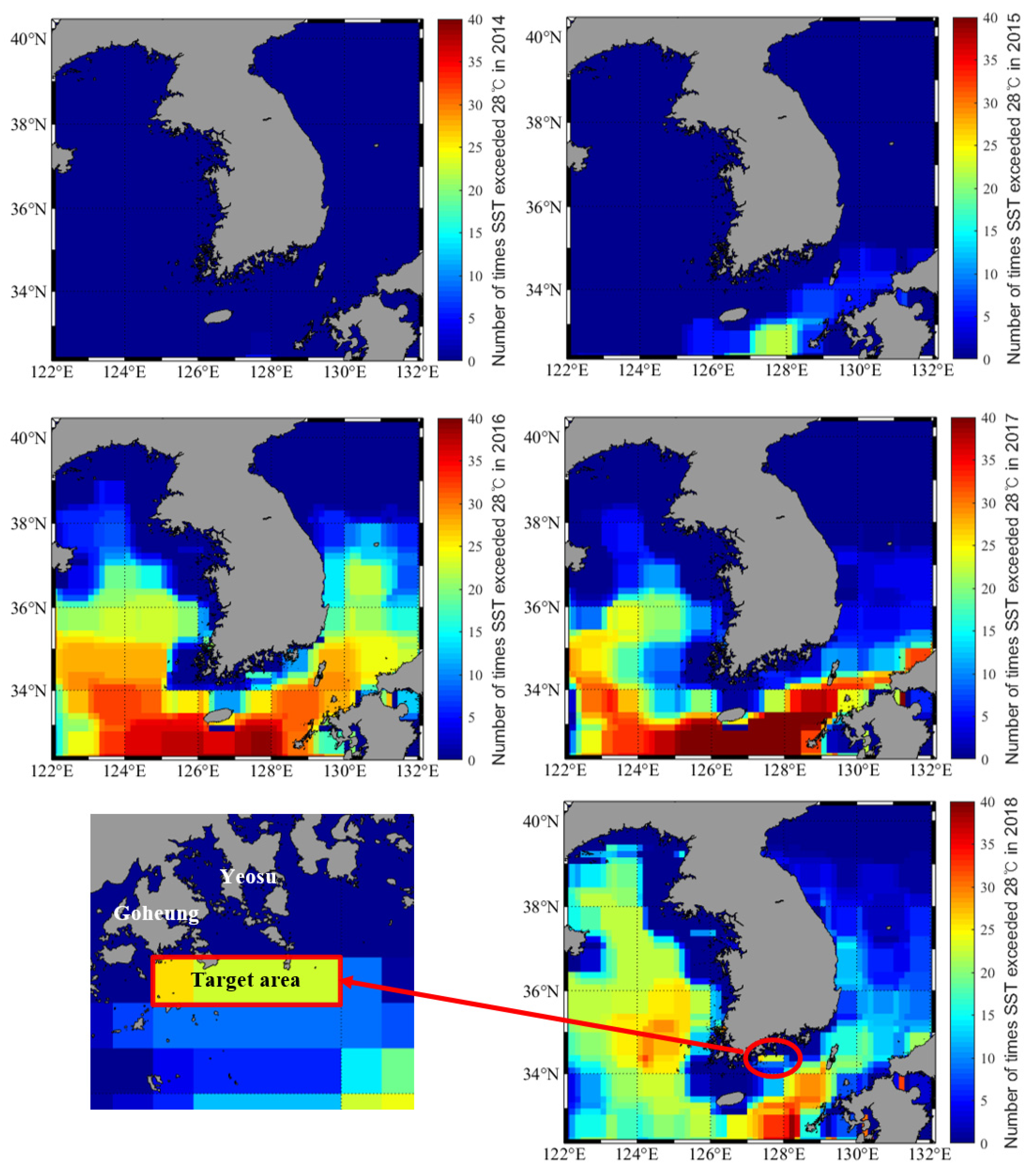
This study used the HWT definition of a SST > 28 °C, which was set by the Korean Ministry of Maritime Affairs and Fisheries [30,31]. Figure 1 shows the number of SSTs exceeding 28 °C in the seas around the Korean Peninsula over the past 5 years and the selected target area for HWT prediction for this study; red corresponds to areas in which HWT was recorded more than 40 times, and blue represents areas in which HWT did not occur.
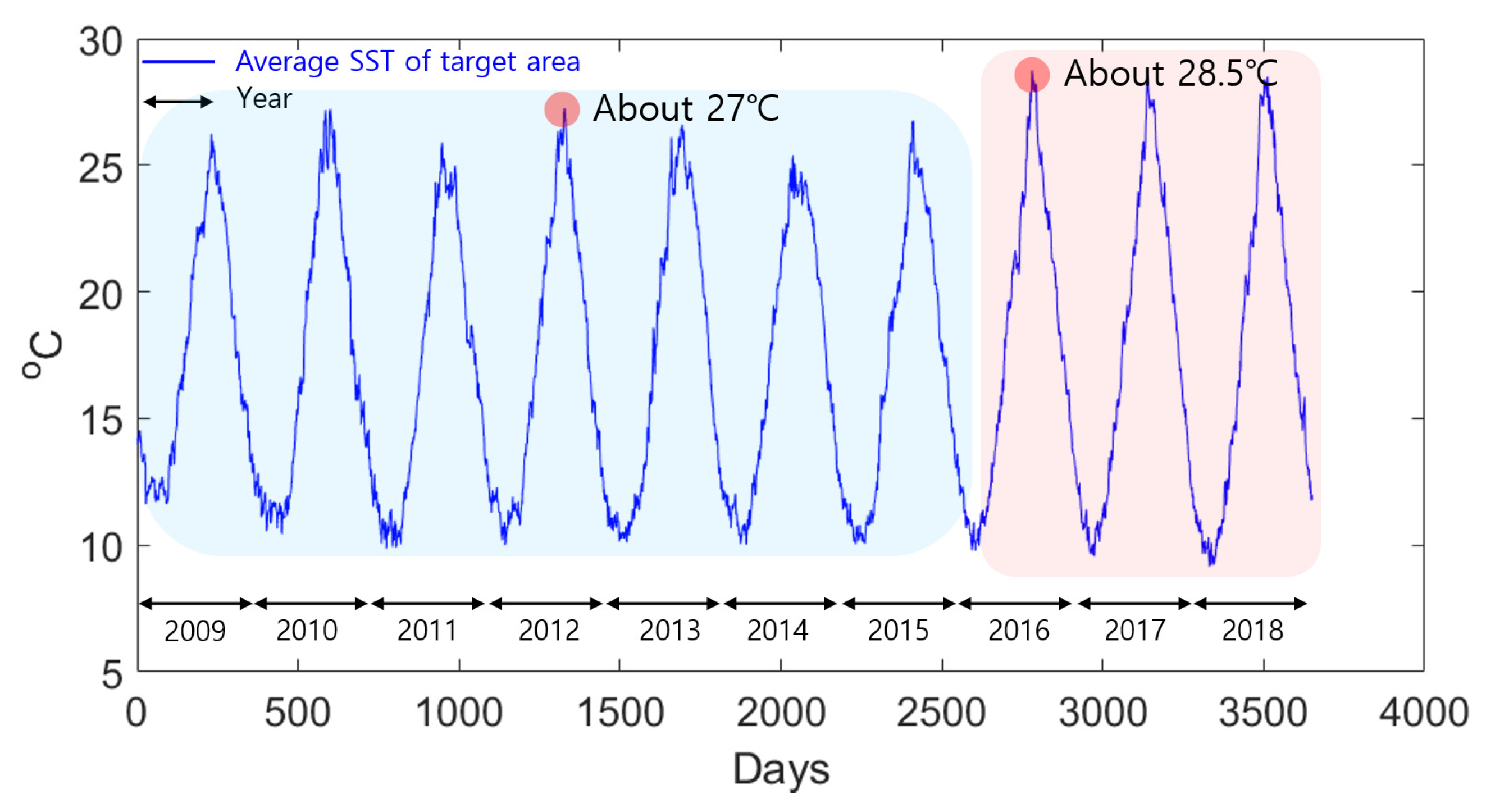
The HWT area and frequency are increasing in coastal areas off the Korean Peninsula due to global warming [32,33]. Figure 2 shows average SSTs for the target area. The maximum SST in the 7-year period between 2009 and 2015 was about 27 °C, and that from 2016 to 2018 (3 years) was about 28.5 °C. Thus, the target area, which contains numerous fish farms, experienced concentrated HWTs during the past 3 years. If HWT events in this area can be forecast in advance, the fishing industry may be able to respond more quickly to moderate the economic damage.
In general, HWTs in Korea are generated for the following reasons. First, as the heat-dome phenomenon becomes stronger due to the strengthening of the power of the North Pacific high pressure and the influence of Tibetan high pressure, the duration and frequency of the heat wave continued to grow [34,35]. Second, the power of the Tsushima warm current, which supplies heat at low latitudes, has been showing strong in the summer in Korea in recent years [36,37]. Third, since the frequency of typhoons that were concentrated in July and August every year decreased, the external force to mix the high-temperature surface sea water with the low-temperature sea water was weakened. For this reason, SST was continuously heated, leading to HWT.
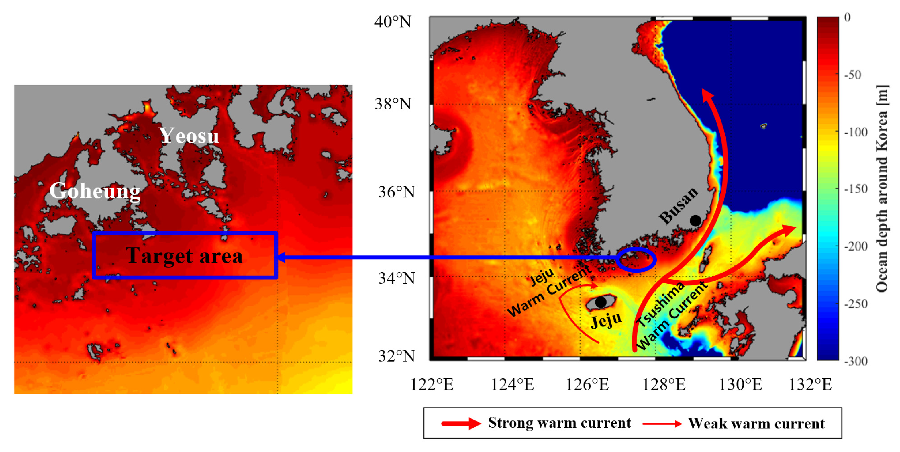
HWTs in Korea are generally caused by the above 3 points. However, since the target area selected in this study is a very shallow area, it is greatly affected by the ocean depth. Figure 3 shows the ocean depth and current flow patterns around Korea. The Kuroshio warm current flows northeast from Philippines to the east coast of Japan, and these warm currents are separated into the Tsushima warm current and the Jeju warm current [38,39]. The Jeju warm current rotates clockwise on Jeju Island and merges with the Tsushima warm current. However, since the target area selected in this study was located on the coast, the effect of these warm current was small. Studies have shown that ocean depth has a significant effect on SST [40,41], and shallow coasts respond quickly to atmospheric changes due to their low heat storage capacity [42]. The ocean depth of the target area is also very shallow, and its SST tends to rise rapidly in midsummer. Therefore, it can be seen that the HWT phenomena occurred frequently in the target area while the HWT phenomena did not occur much in coasts near Busan and Jeju where the ocean depth was deeper and the current flow was faster than the target area.
2.2. Data
SST data were obtained from the ERA5 product released by ECMWF. ERA5 is the fifth-generation ECMWF atmospheric reanalysis of global climate, and is the successor to FGGE reanalysis of the 1980s, which included ERA-15, ERA-40, and ERA-Interim. Reanalysis combines the model with observations to provide a numerical explanation of recent climate and is used by thousands of researchers worldwide. At present, ECMWF provides data such as SST, wind, dewpoint, and snowfall. We focused on ERA5 reanalysis SST data [43,44].
Hourly SST data were provided by ECMWF; we considered the noon measurement of SST to be representative of daily SST values. The SST data format consisted of 721 × 1440 data points, with a spatial resolution of 0.25° latitude and 0.25° longitude. The target coastal area from Goheung to Yeosu selected for SST and HWT prediction included a total of five pixels at a latitude of 34.45°, with a longitude spanning from 127.3 to 128.3°.
Dataset citable as: Copernicus Climate Change Service (C3S): ERA5: Fifth generation of ECMWF atmospheric reanalysis of the global climate. Copernicus Climate Change Service Climate Data Store (CDS), date of access. (https://cds.climate.copernicus.eu/cdsapp#!/dataset/reanalysis-era5-pressure-levels?tab=overview).
3. Methods
3.1. Structure of the LSTM
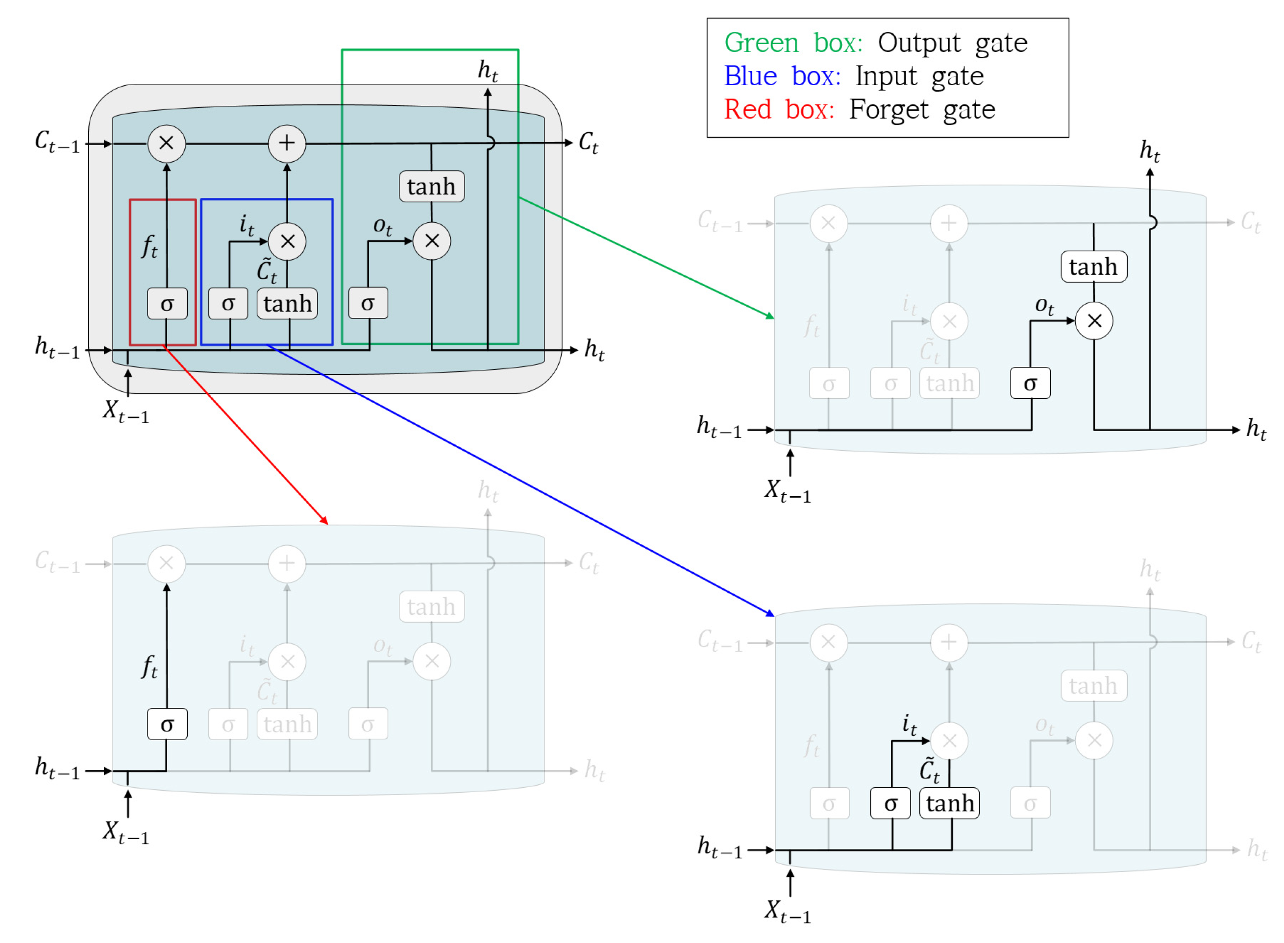
Figure 4 shows the structure of an LSTM. LSTM solves the long-term dependency problem, a disadvantage of the RNN algorithm, using a forget gate. The forget gate allows the previous data to be forgotten if the current data are important; additionally, the previous data are remembered if the current data are unnecessary. The forget gate is calculated as follows:
where is a sigmoid activation function. In previous studies, can use various types of functions, but there are studies using sigmoid functions [45,46], so in this study, the sigmoid function was applied. and are the output of the previous step and the current input, respectively, and and represent the weight and bias values, respectively. If , which is composed of the sigmoid function, approaches 0, the previous data are forgotten; if it approaches 1, the previous data are remembered. The next step, the input gate, determines which of the new data are stored in the cell state:
where the input-gate layer determines which value to update, and the tanh layer creates a new candidate value . By combining the data from these two stages, the model creates a value to update the cell state. The new cell state is available by updating in the past state. The last gate, the output gate, determines what to output:
where represents the new output value.
3.2. LSTM Training Concept
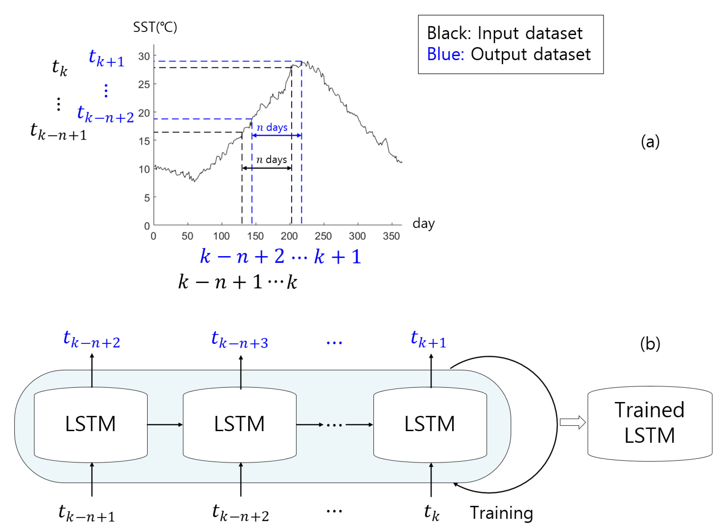
To illustrate the LSTM training concept, consider typical 1-year SST values, as shown in Figure 5a. In this figure, the 1-year SST increased to approximately 30 °C in the summer and decreased to approximately 10 °C in the winter. Especially between days 210 and 250, roughly from July to August, HWTs exceeding 28 °C appeared more frequently. Figure 5b shows a schematic diagram of LSTM training based on input/output (I/O) data pairs. The input dataset used for LSTM training can be expressed as with days of SST data, and the output data can be expressed as , where refers to the SST, and and represent the number of I/O data and the start day of the input data, respectively. The start day of input data was set to be random, to prevent certain parts from being trained.
Once the I/O data pairs are determined and trained, a trained LSTM model can be generated to predict the SST. The important point here was that unused data, i.e., data not used in the LSTM training, should make up the input data of the trained LSTM model; otherwise, the outcome could only be used as an index to judge whether the training was successful but would not be meaningful in predicting future water temperatures.
3.3. SST Prediction Concept using the Trained LSTM Model
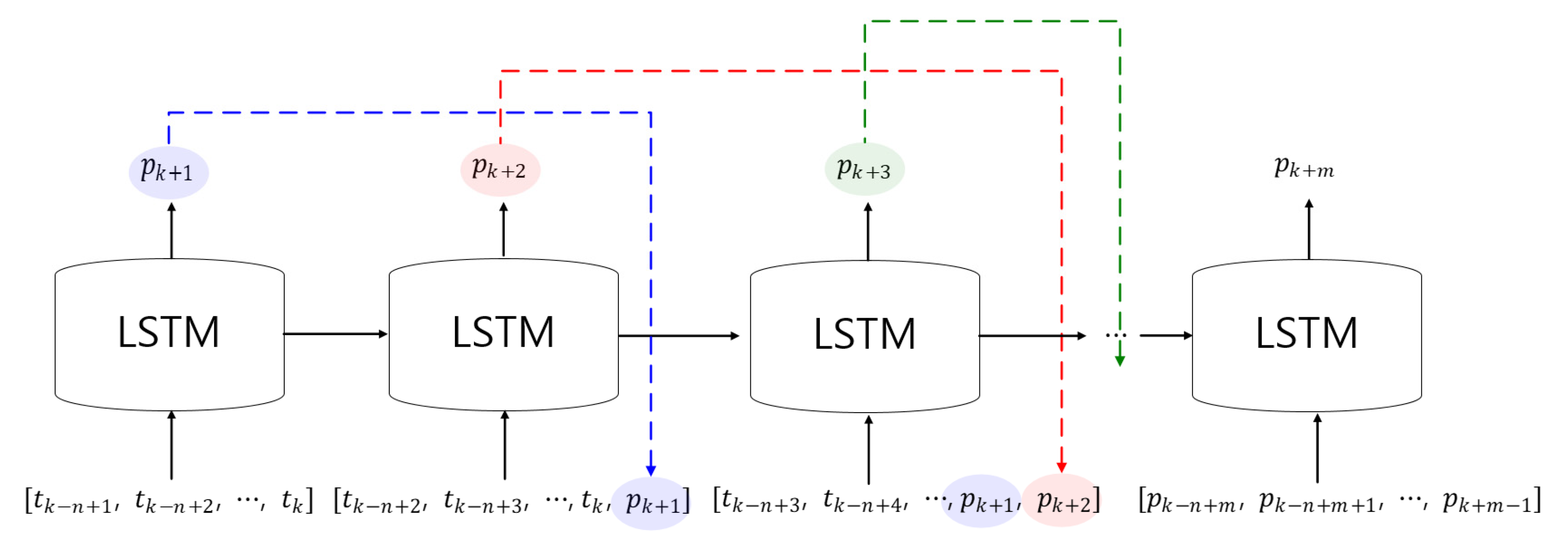
Section 3.3 describes a method for predicting the days SST based on the trained LSTM model. The predicted SST after 1 day was selected as the last component of the output. The SST prediction then proceeded to forecast the SST after m days using the following process.
Figure 6 shows schematic diagrams for predicting SST after days. The key concept is that LSTM’s outputs are reused as an element of the input array to predict after m days. Where is the output of the trained LSTM. To predict the SST after m days the following procedure was used
- (1)
- Extract the predicted SST after 1 day from the trained LSTM.
- (2)
- To predict the SST after 2 days, the predicted SST after 1 day was substituted as the last component of the second input.
- (3)
- Extract the predicted SST after 2 days as a result of step 2.
- (4)
- To predict the SST after 3 days, the predicted SST after 2 days was substituted as the last component of the second input. Here, the predicted SST after 1 day was located before the last component.
- (5)
- Repeat this process times.
By repeating the above procedure, the trained LSTM could generate the predicted SST after days as an output.
3.4. HWT Determination Algorithm and Performance Evaluation
In this study, we assumed a HWT threshold of 28 °C in Korea. So we designed the state transition diagram of the algorithm used to determine HWT occurrence based on this threshold. If the predicted SST was < 28 °C after m days (, then the state was deemed normal; otherwise, the state was changed to HWT. To evaluate the performance of the HWT prediction algorithm, a space analysis of the receiver operating characteristic (ROC) curve was performed. Performance was assessed based on the true positive rate (TPR) or false positive rate (FPR) [47], which were calculated as follows:
where TP, TN, FP, and FN are the numbers of data points representing true positive, true negative, false positive, and false negative cases, respectively. If the outcome from a prediction is positive, and the real value is also positive, then the outcome is referred to as a TP; however, if the real value is negative, then it is called an FP. Conversely, a TN occurs when both the prediction outcome and real value are negative, and a FN is assigned when the prediction outcome is negative and the real value is positive. When the TPR approaches 1 and FPR approaches 0, the prediction performance is excellent; in the ROC space composed of TPR and FPR, the distribution of values in the upper left shows superior prediction performance.
We also performed F1 score analysis to investigate how the HWT prediction algorithm responded to changes in the prediction interval. In statistical analyses, the F1 score represents the harmonic average between precision and sensitivity, as follows [48]:
3.5. Method of SST Prediction Performance Evaluation
To evaluate SST prediction performance, the predicted SST of the trained LSTM model was compared with actual SST data using the coefficient of determination (R2), root mean square error (RMSE), and mean absolute percentage error (MAPE). R2, RMSE, and MAPE were calculated as follows [49]:
where SSTpredicted and SSTreal are the predicted SSTs from the trained LSTM model and ERA5 SST data, and n is the number of samples.
4. Experiments
4.1. LSTM Network for Experiments
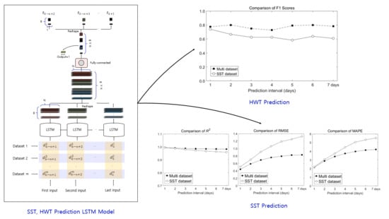
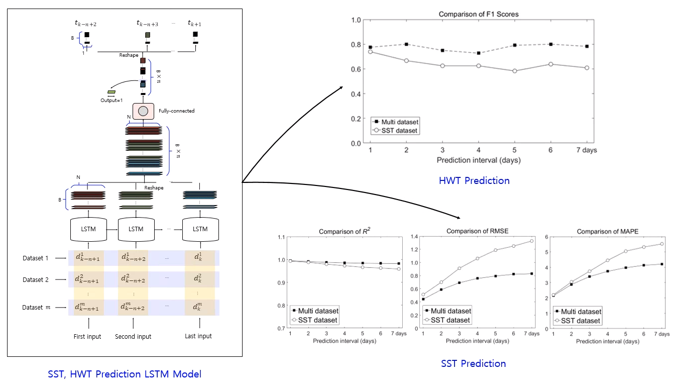
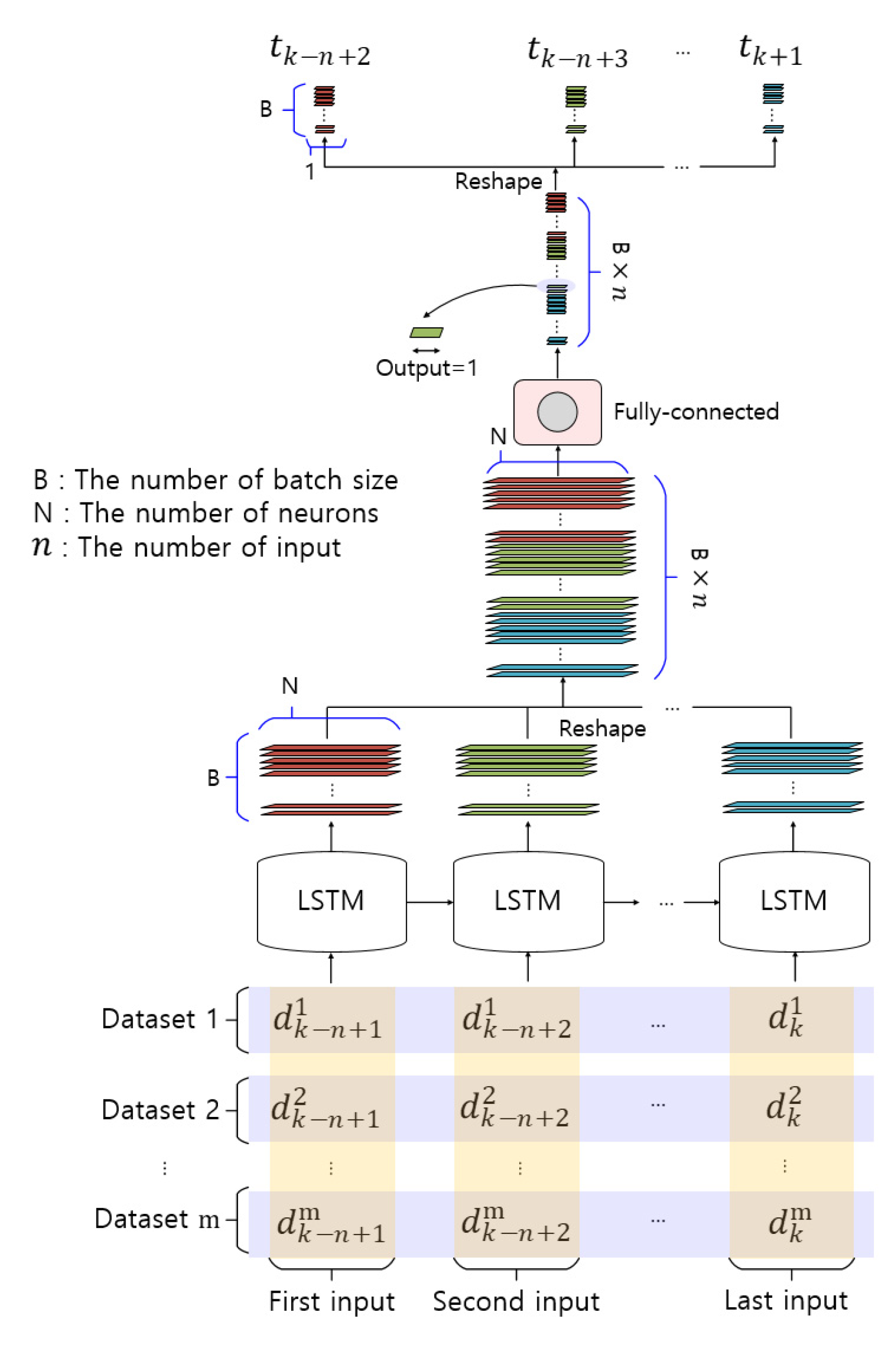
Figure 7 shows the structure of the actual LSTM network used in the experiments to predict the SST after days. B, N, and represent the numbers of batch sizes, neurons, and inputs, respectively. Datasets 1 through are external meteorological data to be reflected during training. To prevent confusion of symbols, used for “after days” is in italics, and m is used to mean the number of datasets. For example, if only SST data are used in training, then dataset 1 becomes SST data, and if SST, wind, and air-temperature data are used, then dataset 1 becomes SST data, dataset 2 becomes wind data, and dataset 3 becomes air-temperature data. As such, the LSTM network was designed as a structure to which desired meteorological data can be continuously added. Each LSTM cell generates an output vector having the form (B, N). However, the output required is a vector having the form (B, 1). To convert the shape of the output, we used the following procedure.
- (1)
- The output vectors of form (B, N) of each LSTM cell with n inputs were stacked in the vector having the form (B × , N).
- (2)
- A fully connected layer with one unit was applied to reshape the vector having the form (B × , N) into a vector having the form (B × , 1; because the fully connected layer is only a layer for dimension reduction, the activation function is not used).
- (3)
- The vector is reduced from the form (B × , 1) into n outputs. Now the output is a vector of form (B × 1).
By performing the steps above, we could obtain the predicted SST value.
4.2. Parameter Values for the Simulation
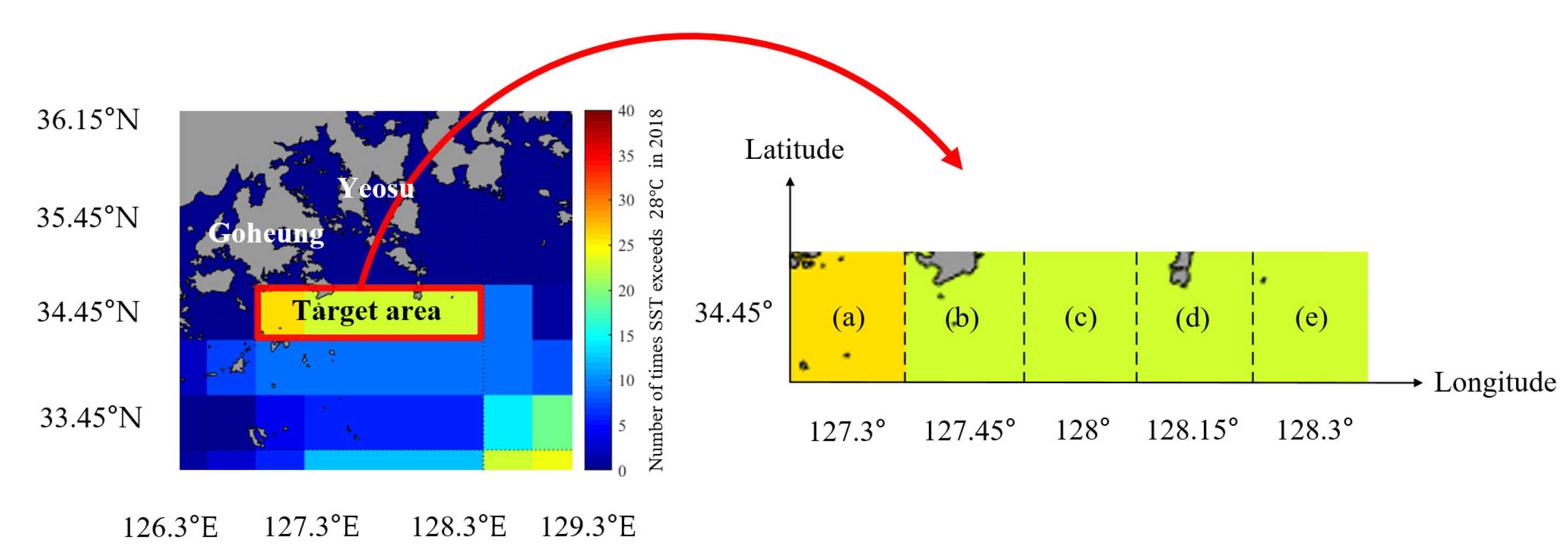
For convenience, the target areas for predicting SSTs from 1 day to days is defined as shown in Figure 8a–e; the parameter values and training data of the LSTM network used in the simulation are presented in Table 1.
Figure 8 shows the target area along the coast from Goheung to Yeosu in Jeollanam-do, which experienced a high occurrence of HWTs. The target area was divided into five areas, designated as a–e in the figure, corresponding to a latitude of 34.45° and longitude spanning from 127.3 to 128.3°. The color shown for each area corresponds to the number of HWT occurrences in 2018, as given in Figure 1.
The simulation was conducted using only one type of training data (SST) and three types of data (SST, wind, and air temperature); the latter case is referred to as the multi dataset. In session 2 said that HWTs in Korea are caused by strong Tsushima warm current, typhoons that were not concentrated in July and August, and heat wave caused by the heat-dome. Therefore, air temperature and wind that can be used as indicators of heat wave and typhoon were added to the multi dataset.
We used data collected during the past 10 years (2008–2017) to predict SSTs in 2018. The SST dataset (m = 1) contained 3650 input data and the multi dataset (m = 3) contained 3650 × 3 input data. However, both datasets resulted in 3650 output data because daily SSTs were the only output.
Table 1 shows the parameter values and the I/O datasets for training the LSTM network used in the simulation. To perform the simulation, the number of batch sizes B, the number of neurons N, and the number of inputs were selected as 30, 100, and 30, respectively. The cost function, which is an indicator of the performance of the model, was based on the mean square error. Minimizing the cost function means that the error between the LSTM output and the correct answer is small. The Adam optimizer was used as the optimization function to minimize the cost function.
As a result of experiments as the number of neurons and training data were varied, it was determined that 100 neurons and 3650 training data were appropriate. For better understanding, the sensitivity of the model to various experiments is shown in Appendix A’s Table A1.
To predict the SSTs in the five areas shown in Figure 8a–e, the LSTM was trained using 10 years of data for the individual areas, thus effectively creating a trained LSTM model for that particular area. The trained LSTM model was then used to predict the SSTs in 2018. Since the SST prediction year was 2018, 335 data were needed (30 input data were required as the initial input for the LSTM model).
4.3. Results
4.3.1. Results Obtained Using only SST Input Data
In this simulation, SSTs were predicted using only the widely used SST dataset for LSMT training. The simulation was conducted for area (a). To calculate R2, RMSE, and MAPE, the number of samples was set to 335; only the data between 31 and 365 in 2018 were compared, in which the head data were eliminated for improved accuracy. The input of the trained LSTM model required SST data from 30 samples; thus, the SST data from these 30 samples were eliminated from the data head (i.e., used data elimination as discussed earlier).
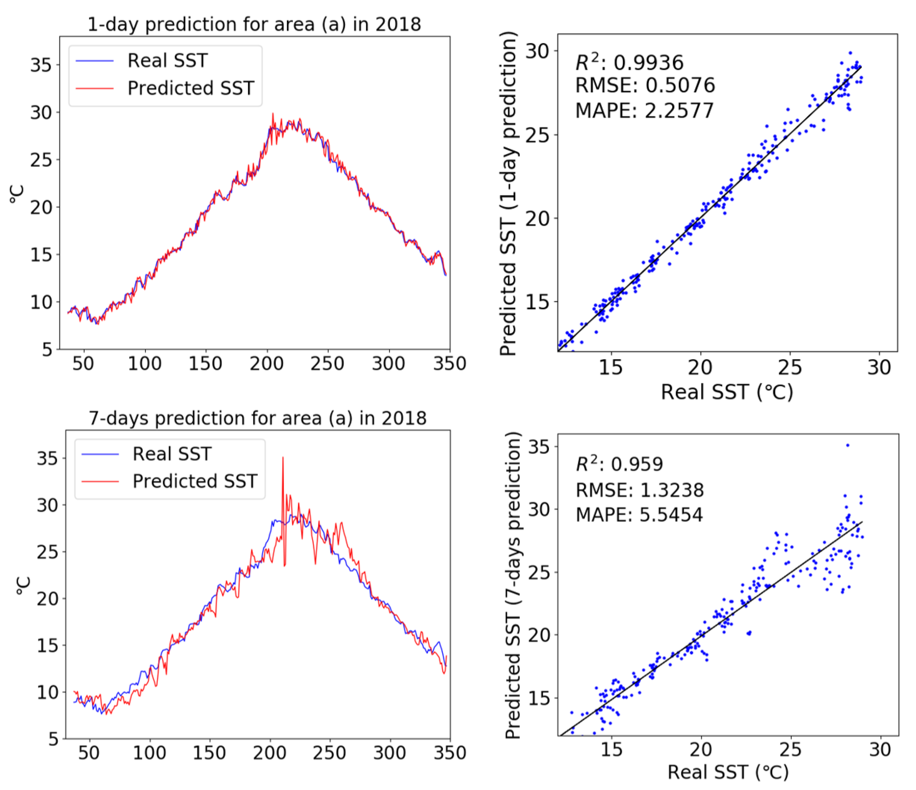
Figure 9 shows a comparison of real and predicted SSTs produced using only the SST dataset as input for area (a) in 2018; scatter plots were used to evaluate the performance of the trained LSTM model. Simulation results revealed a similar trend between the real and predicted SST data for SST prediction after 1 day. The results of the scatter plot analysis also showed that the LSTM model using only the SST dataset as input was very accurate. In the SST prediction after 1 day, the R2, RMSE, and MAPE values between the predicted SST and real data were 0.9936, 0.5076, and 2.2577, respectively. However, looking at the SST prediction after 7 days, the overall trend showed a lower accuracy than the prediction after 1 day, with R2, RMSE, and MAPE values (0.959, 1.3238, and 5.5454, respectively) between the predicted SST and real data.
4.3.2. Results Obtained Using the Multi Dataset as Input
When only SST data were used as input, the SST prediction performance of the LSTM network rapidly deteriorated as the prediction interval increased. This result occurred because external meteorological data, which have a large influence on SSTs, were not used as input. To confirm that external meteorological data can improve SST prediction performance, we predicted SSTs using the multi dataset composed of SST, wind and air temperature datasets. The reanalysis dataset of ERA5 on the wind and air temperature were obtained in the same way as in Section 2.2.
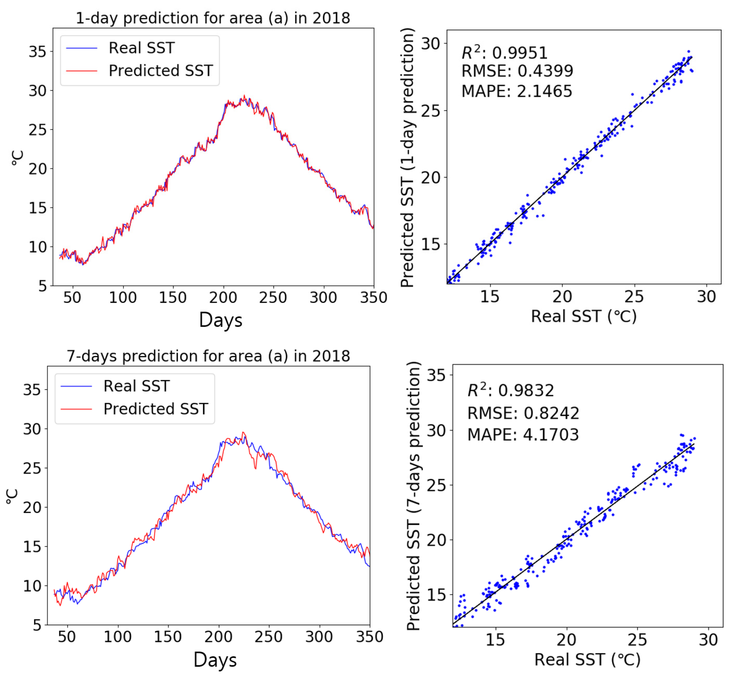
Figure 10 compares real and predicted SST results produced using the multi dataset as input for area (a) in 2018. Scatter plots were used to evaluate the performance of the trained LSTM model. After 1 day, SST predictions did not differ significantly between the two cases because the prediction interval was very short. However, after 7 days, the overall trend produced using the multi dataset was much more faithful to the observation data, with less variation than shown in the result produced using only the SST input dataset. Thus, the external meteorological data had a great influence on SST prediction performance. The R2, RMSE, and MAPE values between the predicted and real SST were 0.9832, 0.8242, and 4.1703, respectively, which indicated that the multi dataset improved our SST predictions.
5. Performance Evaluation
5.1. Comparison of Performance Between SST and Multi Dataset Inputs
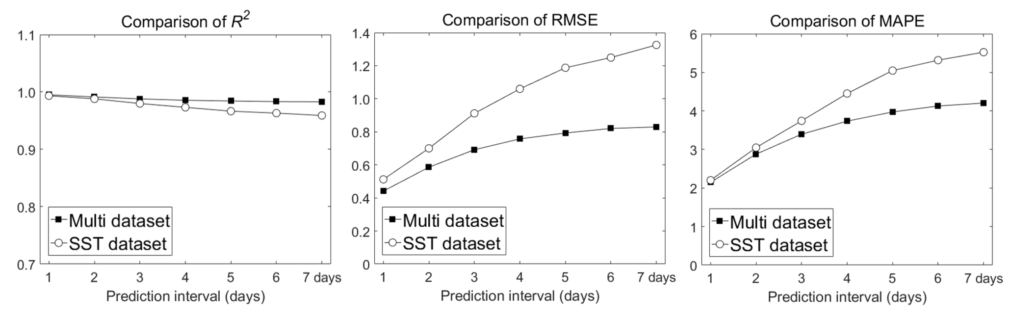
Figure 11 shows a comparison of R2, RMSE, and MAPE values between LSTM results produced using the SST and multi datasets as input, for different prediction intervals. For both input cases, the prediction performance of the LSTM model decreased as the prediction interval increased. However, the multi dataset led to better performance than the SST dataset in terms of R2, RMSE, and MAPE. Thus, to accurately predict SSTs, SST and external meteorological data (wind and air temperature) are important factors.
Both models had similar performances in predicting SST after 1 day, therefore the SST dataset may be used for predicting 1 day. When using the SST dataset, the number of input data is three times less than that of the multi dataset, which has the advantage of shortening the training time. However, the processing (prediction) time is similar because both trained models were used to predict the SST. Therefore, it would be desirable to use the multi dataset with superior prediction performance as the prediction interval increases.
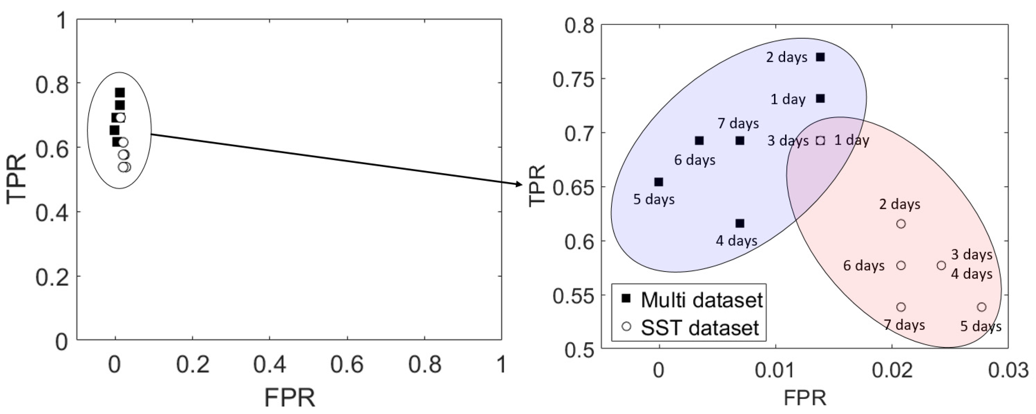
Figure 12 shows the ROC space and plots of HWT occurrence predictions from 1 to 7 days using the TPR and FPR. For both input cases, the calculated values plotted in the upper left corner, which indicates that the proposed algorithm was performed correctly, with the multi-dataset case showing better performance. Model performance was particularly good in terms of the FPR because SST exceeded 28 °C during the summer months of the study year. TN is the value when the real and predicted SSTs do not exceed 28 °C. Therefore, it is necessary to focus on the TPR with respect to HWT prediction.
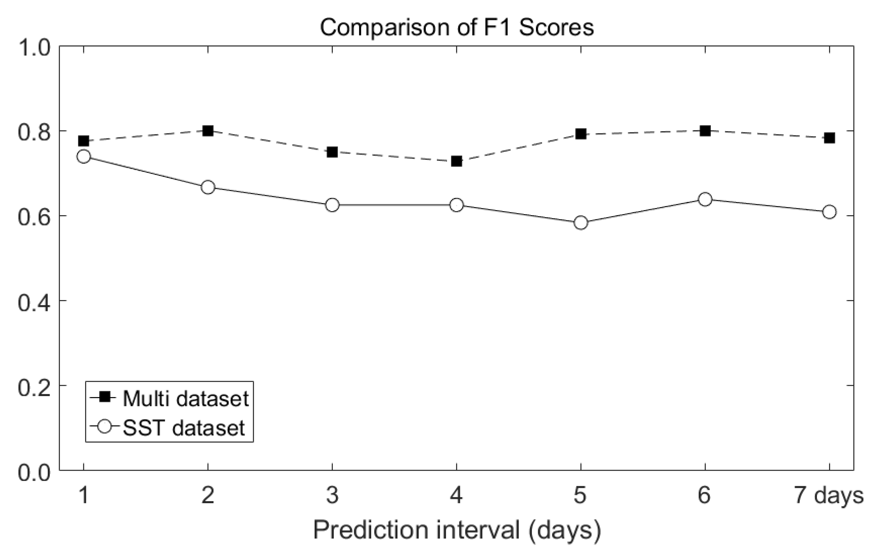
F1 score is a statistical analysis method that evaluates the performance of the model when the data has an unbalanced structure. The frequency of occurrence of HWTs assumed in this study corresponds to this structure because it is concentrated in the summer of a year. Therefore, the performance of the proposed model was evaluated through the F1 score using the harmonic average rather the arithmetic average between precision and sensitivity. Figure 13 shows the comparison of F1 scores obtained using the two input datasets. For the HWT occurrence results obtained using only the SST dataset, the F1 score decreased from 0.8 to 0.6 as the prediction interval increased. However, for the multi-dataset case, even when the prediction interval increased, the F1 score remained constant at about 0.8. In terms of F1 score, it can be seen that the model using multi dataset had better performance in predicting HWTs than the case using the SST dataset.
Additionally, in order to confirm that the model proposed in this study could be applied not only to the target area but also to other areas, an additional experiment was conducted on the sea area near Jeju where HWT occurs frequently. The performance evaluation for this area is shown in Appendix A’s Figure A2.
5.2. Performance Comparison with ECMWF Forecast Data
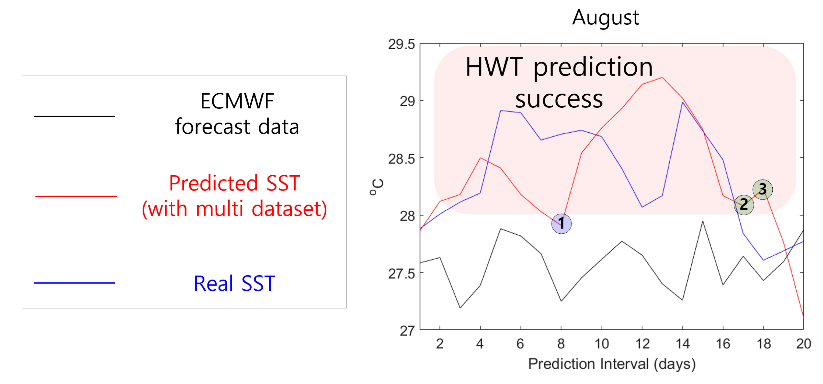
To verify the performance of the SST prediction model using the multi dataset, the results of the proposed model were compared with those produced using ECMWF forecast data. The ECMWF forecast data provide predicted SSTs every 6 h starting from midnight on the first of every month and spatial resolution is composed of 1°. For accurate comparative analysis, we used noon forecast data (to match our output data) for the region located at latitude of 34° and longitude of 127° closest to area (a). Since the SST prediction model proposed in this study requires 30 days of data as an initial input, January was excluded from the comparison. For area (a), the HWT intensively occurred 18 times in August 2018. Therefore, in Figure 14, the performance of the proposed model and ECMWF forecast data was compared and analyzed by increasing the prediction interval from 7 to 20 days. Additionally, for the remaining months where HWT was not concentrated, the prediction interval was set to 7 days, and its performance was represented in Appendix A’s Figure A3.
ECMWF forecast dataset citable as: Copernicus Climate Change Service (C3S): Copernicus Climate Change Service Climate Data Store (CDS), date of access. (https://cds.climate.copernicus.eu/cdsapp#!/dataset/seasonal-original-single-levels?tab=overview).
Figure 14 shows the predicted SST results for the first to twentieth days of August 2018 obtained using the proposed model with multi-dataset input and ECMWF forecast data. SST predictions for August 2018 demonstrate that the proposed model showed superior performance to ECMWF forecast data. The ECMWF forecast data failed to predict HWTs, whereas the proposed model predicted HWT in most prediction interval except for blue circle 1 and green circle 2 and 3. Blue circle 1 indicates that the HWT prediction failed, and green circle 2 and 3 indicate that HWT was determined even though HWT did not occur. These results indicate that the proposed model will be helpful for SST or HWT predictions in the field.
6. Conclusions
In this study, we proposed a deep-learning-based SST and HWT prediction methodology to prevent mass mortality of aquaculture fish caused by HWTs. To predict SSTs and HWTs, we applied an RNN-based LSTM model for the coastal area between Goheung to Yeosu, Jeollanam-do, Korea, which suffered great economic damage due to HWTs in 2018. To train the SST prediction model, we used daily noon SST data provided by the ECMWF.
Previous studies have predicted SSTs by training deep-learning-based prediction models using only large SST datasets. However, these methods have limited accuracy because they do not take external meteorological factors into account. Therefore, in this study, we added external meteorological data (wind and air temperature) as input for the SST prediction model. The SST prediction model was designed to predict the SST after 1 day; to obtain predictions over a period of days, this result was placed at the end of the next input, and the method was repeated.
First, the LSTM model was trained using a 10-year SST dataset for the study area. The model’s 1 day SST prediction performance was excellent, but decreased as the prediction interval increased because predicted SSTs formed the basis of each subsequent day’s predictions. Prediction of HWT occurrence was also evaluated based on TPR, FPR, and F1 score values. As the prediction interval increased, the prediction performance decreased overall.
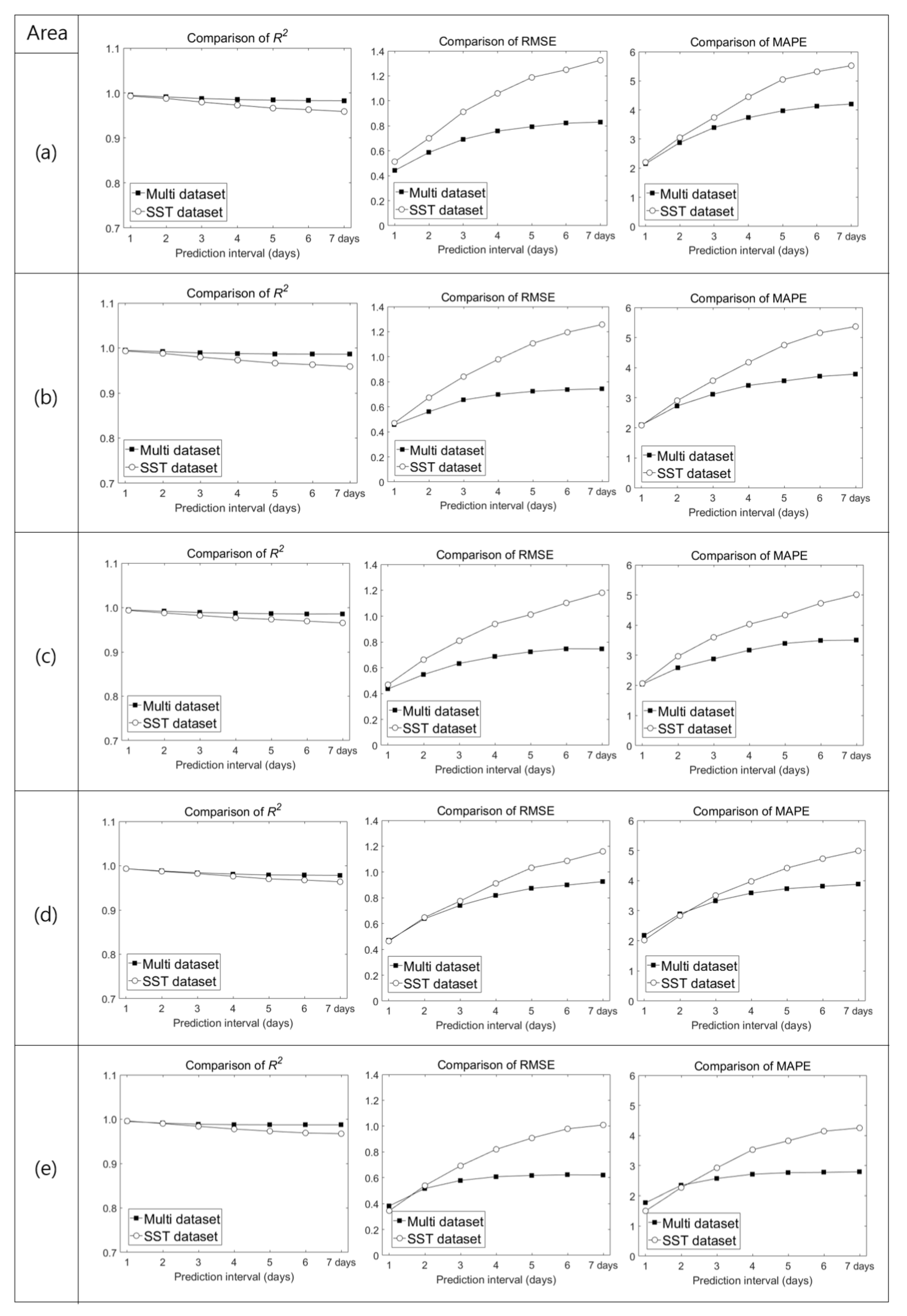
To compensate for the decreases in the SST and HWT prediction performance as the prediction interval increased, we changed the training dataset. In the initial experiment, we used a training dataset composed of SST data only; we subsequently created a multi dataset composed of wind, air-temperature, and SST data. Our results obtained using the multi dataset were superior to those obtained using the SST training dataset, in area (a) as well as in other areas (b–e), according to R2, RMSE, and MAPE values. Model performance in each study area (b–e) is described in Appendix A’s Figure A1. HWT was also better predicted using the multi dataset than using the SST dataset as input because wind and air temperature play important roles in contributing to SSTs. Further analyses of the impact of wind and air temperature input data on model training would improve the accuracy of SST prediction.
The deep-learning-based SST prediction methodology proposed in this paper shows very accurate performance when the prediction interval is short but deteriorates as the prediction interval increases. For this reason, it is possible to predict SSTs over a short period in real environments; however, the method is limited in its long-term forecasting ability. In this study, we used a multi dataset consisting of a 3D array as input for the LSTM model to predict the SST after m days. In a future study, we intend to train the LSTM model using multi-dimensional arrays (m ≥ 3) that include ocean currents, air pressure, heat flux, and salinity data in addition to wind and air-temperature data, which directly affect SST. We also plan to analyze how each type of meteorological data affects SST prediction performance to create an optimal training dataset for the model. These modifications are expected to improve the accuracy of the generated prediction model to improve prediction performance for days.
We have a plan to contribute to the prevention of damage to the Korean aquaculture industry by recommending the SST and HWT prediction model using the multi dataset proposed in this study to Korean Ministry of Maritime Affairs and Fisheries and related organizations.
Author Contributions
Conceptualization, H.Y. and J.K.; methodology, H.Y.; software, M.K.; validation, H.Y., J.K. and M.K.; formal analysis, M.K.; investigation, M.K.; resources, M.K.; data curation, M.K.; writing (original draft preparation), M.K.; writing (review and editing), H.Y., J.K. and M.K.; visualization, M.K.; supervision, H.Y. and J.K.; project administration, H.Y. and J.K.; funding acquisition, H.Y. All authors have read and agreed to the published version of the manuscript.
Funding
This research was supported by a National Research Foundation of Korea (NRF) grant funded by the Korean government (MSIT) (no. 2018R1D1A1B07049261) and by the projects “Technology Development for Practical Applications of Multi-Satellite Data to Maritime Issues” and “Development of the Integrated Data Processing System for GOCI-II”, which were funded by the Ministry of Ocean and Fisheries, Korea.
Acknowledgments
The authors acknowledge the assistance of the Ocean Satellite ICT Convergence (OSIC) Laboratory (http://osic.kosc.kr/) and graduate students of the Intelligence Control Laboratory of Korea Maritime and Ocean University (KMOU).
Conflicts of Interest
The authors declare no conflict of interest.
Appendix A

Table A1.
Sensitivity of LSTM model to changes in the number of neurons and training data.
| Number of Training Data | Number of Neurons | Prediction Interval | Prediction Performance | |||
|---|---|---|---|---|---|---|
| SST | HWT | |||||
| R2 | RMSE | MAPE | F1 Score | |||
| 1825 past 5 year (2013–2017) | 50 | 1 | 0.9883 | 0.693 | 2.5784 | 0.5128 |
| 7 | 0.8785 | 2.2615 | 7.0832 | 0.057 | ||
| 1825 past 5 year (2013–2017) | 100 | 1 | 0.9926 | 0.5488 | 2.4148 | 0.7391 |
| 7 | 0.9538 | 1.3789 | 5.7256 | 0.44 | ||
| 1825 past 5 year (2013–2017) | 150 | 1 | 0.9946 | 0.4728 | 2.1033 | 0.7391 |
| 7 | 0.9707 | 1.0953 | 5.134 | 0.44 | ||
| 3650 past 10 year (2008–2017) | 50 | 1 | 0.9921 | 0.5677 | 2.5429 | 0.66 |
| 7 | 0.9564 | 1.3059 | 5.6304 | 0.58 | ||
| 3650 past 10 year (2008–2017) | 100 | 1 | 0.9936 | 0.5076 | 2.2577 | 0.7391 |
| 7 | 0.959 | 1.3238 | 5.5454 | 0.6086 | ||
| 3650 past 10 year (2008–2017) | 150 | 1 | 0.9949 | 0.4542 | 2.0829 | 0.76 |
| 7 | 0.961 | 1.251 | 5.736 | 0.6249 | ||
| 5475 past 15 year (2003–2017) | 50 | 1 | 0.9962 | 0.398 | 1.8067 | 0.7272 |
| 7 | 0.9788 | 1.0027 | 5.0365 | 0 | ||
| 5475 past 15 year (2003–2017) | 100 | 1 | 0.9922 | 0.5696 | 2.6503 | 0.66 |
| 7 | 0.9616 | 1.2514 | 5.7366 | 0.4571 | ||
| 5475 past 15 year (2003–2017) | 150 | 1 | 0.9937 | 0.5065 | 2.375 | 0.69 |
| 7 | 0.9649 | 1.2011 | 5.6122 | 0.51 | ||
Table A1 is the result of comparing the SST and HWT prediction performance according to the changes in the number of neurons and the number of training data. Except for the red background with the smallest number of neurons and training data, it can be seen that the similar accuracy in terms of SST prediction performance. However, in this study, not only SST prediction but also HWT prediction was one of the main purposes, therefore we tried to select the numbers of neurons and training data that satisfied both SST and HWT prediction performances.
As a result of experiments for 9 cases, when the number of neurons was small (gray background), the F1 score values indicating HWT prediction performance tended to be low. In addition, it was confirmed that the F1 score value was also low when there were a lot of past data not related to the current pattern (blue box) and when a sufficient amount of training data was not included (green box). Therefore, in this study, considering the above three cases, among red box with similar HWT and SST prediction performance, we selected a blue background with 100 neurons and 10 year’s training data.
Appendix B
Figure A1.
RMSE and MAPE values between LSTM results produced using the SST and multi datasets as input, for different areas.
Figure A1.
RMSE and MAPE values between LSTM results produced using the SST and multi datasets as input, for different areas.

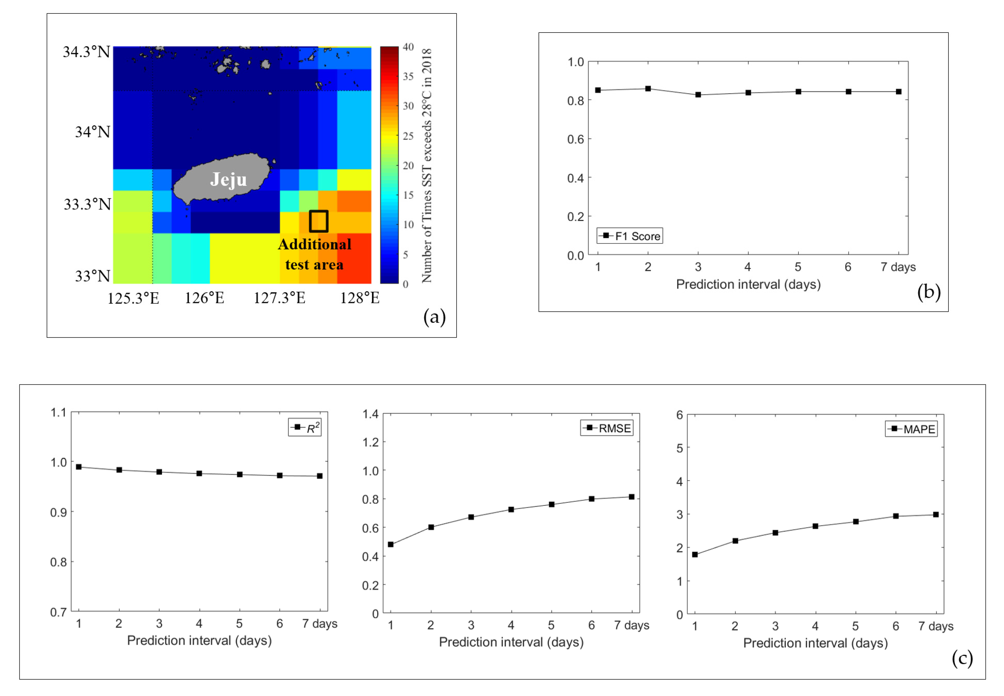
Figure A2.
HWT and SST prediction performance for additional test area using multi dataset. (a) Area selected for further experiments. (b) F1 score values for additional test area. (c) R2, RMSE, and MAPE values for the additional test area.
Figure A2.
HWT and SST prediction performance for additional test area using multi dataset. (a) Area selected for further experiments. (b) F1 score values for additional test area. (c) R2, RMSE, and MAPE values for the additional test area.

Figure A2 is the result of evaluating HWT and SST prediction performance by applying the proposed model (multi-dataset) for additional test area. Figure A2a shows the sea area near Jeju where HWT is generated frequently, and the area selected for an additional test is marked with a black box. Figure A2c shows the value of R2, RMSE, and MAPE according to the prediction interval. It can be seen that the performance was degraded as the prediction interval increases but the proposed model’s performance was similar to that of Appendix B. In Figure A2b, it be seen that the F1 score also remained constant at about 0.8 as the prediction interval increased. Through these results, it was confirmed that the model proposed in this study had the ability to predict HWT not only in the target area but also in other areas.
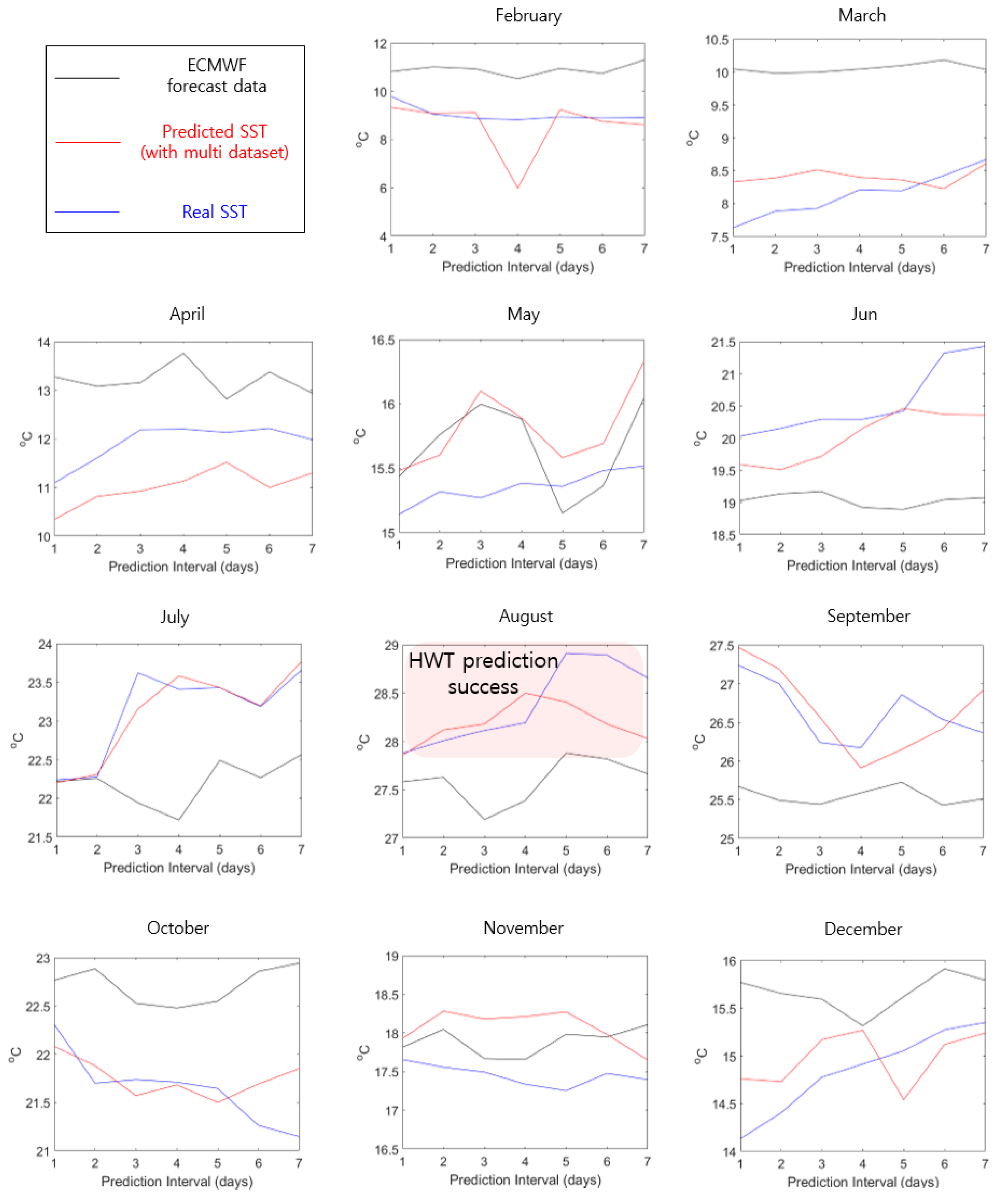
Figure A3.
Comparison of SST prediction performance for August between the proposed model (with multi-dataset input) and European Center for Medium-Range Weather Forecast (ECMWF) forecast data.
Figure A3.
Comparison of SST prediction performance for August between the proposed model (with multi-dataset input) and European Center for Medium-Range Weather Forecast (ECMWF) forecast data.

Figure A3 shows the predicted SST results for the first to seventh day of each month (excluding January) of 2018 obtained using the proposed model with the multi-dataset input and ECMWF forecast data. SST predictions for February to March, June to October, and December demonstrated that the proposed model showed excellent performance. However, in other months, the performance of the proposed model was similar to or slightly inferior to that of ECMWF forecast data. Even when the performance of the proposed model was poor, the difference was as little as about +0.5 °C. From February to December, the difference between the real SST and ECMWF forecast data was 1.9 °C in average, and the difference from the proposed model (with multi dataset) was 0.45 °C on average. These results show that the accuracy of SST prediction was about 4 times better than the ECMWF forecast data.
References
- Hochreiter, S.; Schmidhuber, J. Long short-term memory. Neural Comput. 1997, 9, 1735–1780. [Google Scholar] [CrossRef] [PubMed]
- Schmidhuber, J. Deep learning in neural networks: An overview. Neural Netw. 2015, 61, 85–117. [Google Scholar] [CrossRef] [PubMed] [Green Version]
- Alistair, J.H.; Lisa, V.A.; Sarah, E.P.; Dan, A.S.; Sandra, C.S.; Eric, C.J.; Jessica, A.B.; Michael, T.B.; Markus, G.D.; Ming, F.; et al. A hierarchical approach to defining marine heatwaves. Prog. Oceanogr. 2016, 141, 227–238. [Google Scholar]
- Vitart, F.; Andrew, W.R. The sub-seasonal to seasonal prediction project (S2S) and the prediction of extreme events. Clim. Atmos. Sci. 2018, 1, 1–7. [Google Scholar] [CrossRef] [Green Version]
- Those Who Come Along the Heat… Fishermen Suffered 100 Billion Damage in 10 years. Available online: https://news.joins.com/article/23543775 (accessed on 5 August 2019).
- Balmaseda, M.A.; Mogensen, K.; Weaver, A.T. Evaluation of the ECMWF ocean reanalysis system ORAS4. R. Meteorol. Soc. 2013, 139, 1132–1161. [Google Scholar] [CrossRef]
- Stockdale, T.N.; Anderson, D.L.T.; Balmaseda, M.A.; Doblas-Reyes, F.; Ferranti, L.; Mogensen, K.; Palmer, T.N.; Molteni, F.; Vitart, F. ECMWF seasonal forecast system 3 and its prediction of sea surface temperature. Clim. Dyn. 2011, 37, 455–471. [Google Scholar] [CrossRef]
- Peckham, S.E.; Smirnova, T.G.; Benjamin, S.G.; Brown, J.M.; Kenyon, J.S. Implementation of a digital filter initialization in the WRF model and its application in the Rapid Refresh. Mon. Weather Rev. 2016, 144, 99–106. [Google Scholar] [CrossRef]
- Phillips, N.A. A coordination system having some special advantages for numerical forecasting. J. Meteor. 1957, 14, 184–185. [Google Scholar] [CrossRef] [Green Version]
- Weisman, M.L.; Davis, C.; Wang, W.; Manning, K.W.; Klemp, J.B. Experiences with 0–36-h explicit convective forecast with the WRF-ARW model. Am. Meteorol. Soc. 2008, 23, 1495–1509. [Google Scholar] [CrossRef]
- Skamarock, W.C.; Klemp, J.B.; Dudhia, J.; Gill, D.O.; Barker, D.M.; Wang, W.; Powers, J.G. A Description of the Advanced Research WRF Version 2; NCAR Tech; Note NCAR/TN468 + STR; National Center for Atmospheric Research: Boulder, CO, USA, 2005; p. 88. [Google Scholar]
- Gröger, M.; Dieterich, C.; Meier, M.H.E.; Schimanke, S. Thermal air–sea coupling in hindcast simulations for the North Sea and Baltic Sea on the NW European shelf. Tellus A 2015, 67, 26911. [Google Scholar] [CrossRef] [Green Version]
- Liu, Y.; Fu, W. Assimilating high-resolution sea surface temperature data improves the ocean forecast potential in the Baltic Sea. Ocean Sci. 2018, 14, 525–541. [Google Scholar] [CrossRef] [Green Version]
- Ba, A.N.N.; Pogoutse, A.; Provart, N.; Moses, A.M. NLStradamus: A simple hidden Markov model for nuclear localization signal prediction. BMC Bioinform. 2009, 10, 202. [Google Scholar]
- Berliner, L.M.; Wikle, C.K.; Cressie, N. Long-lead prediction of Pacific SSTs via Bayesian dynamic modeling. Am. Meteorol. Soc. 2000, 13, 3953–3968. [Google Scholar] [CrossRef] [Green Version]
- Johnson, S.D.; Battisti, D.S.; Sarachik, E.S. Empirically derived Markov models and prediction of tropical Pacific sea surface temperature anomalies. Am. Meteorol. Soc. 2000, 13, 3–17. [Google Scholar] [CrossRef] [Green Version]
- Lins, I.D.L.; Araujo, M.; Moura, M.D.C.; Silva, M.A.; Droguett, E.L. Prediction of sea surface temperature in the tropical Atlantic by support vector machines. Comput. Stat. Data Anal. 2013, 61, 187–198. [Google Scholar] [CrossRef]
- Li, Q.J.; Zhao, Y.; Liao, H.L.; Li, J.K. Effective forecast of Northeast Pacific sea surface temperature based on a complementary ensemble empirical mode decomposition-support vector machine method. Atmos. Ocean. Sci. Lett. 2017, 10, 261–267. [Google Scholar] [CrossRef] [Green Version]
- Patil, K.; Deo, M.C. Prediction of sea surface temperature by combining numerical and neural techniques. Am. Meteorol. Soc. 2016, 33, 1715–1726. [Google Scholar] [CrossRef]
- Kumar, J.; Goomer, R.; Singh, A.K. Long Short Term Memory Recurrent Neural Network (LSTM-RNN) Based Workload Forecasting Model For Cloud Datacenters. Procedia Computer Sci. 2018, 125, 676–682. [Google Scholar] [CrossRef]
- Tangang, F.T.; Hsieh, W.W.; Tang, B. Forecasting the equatorial Pacific sea surface temperatures by neural network models. Clim. Dyn. 1997, 13, 135–147. [Google Scholar] [CrossRef]
- Abdel-Nasser, M.; Mahmoud, K. Accurate photovoltaic power forecasting models using deep LSTM-RNN. Neural Comput. Appl. 2019, 31, 2727–2740. [Google Scholar] [CrossRef]
- Wu, Y.; Yuan, M.; Dong, S.; Lin, L.; Liu, Y. Remaining useful life estimation of engineered systems using vanilla LSTM neural networks. Neurocomputing 2018, 275, 167–179. [Google Scholar] [CrossRef]
- Yang, B.; Sun, S.; Li, J.; Lin, X.; Tian, Y. Traffic flow prediction using LSTM with feature enhancement. Neurocomputing 2019, 332, 320–327. [Google Scholar] [CrossRef]
- Zhang, Y.; Xiong, R.; He, H.; Pecht, M.P. Long short-term memory recurrent neural network for remaining useful life prediction of lithium-ion batteries. IEEE Trans. Veh. Technol. 2018, 67, 5695–5705. [Google Scholar] [CrossRef]
- Ahn, S.M.; Chung, Y.J.; Lee, J.J.; Yang, J.H. Korean sentence generation using phoneme-level LSTM language model. Korea Intell. Inf. Syst. 2017, 6, 71–88. [Google Scholar]
- Chaudhary, V.; Deshbhratar, A.; Kumar, V.; Paul, D. Time series-based LSTM model to predict air pollutant concentration for prominent cities in India. In Proceedings of the 1st International Workshop on Utility-Driven Mining, Bejing, China, 31 July 2018; pp. 17–20. [Google Scholar]
- Wang, H.; Dong, J.; Zhong, G.; Sun, X. Prediction of sea surface temperature using long short-term memory. IEEE Geosci. Remote Sens. Lett. 2017, 14, 1745–1749. [Google Scholar]
- Liu, J.; Zhang, T.; Han, G.; Gou, Y. TD-LSTM: Temporal dependence-based LSTM networks for marine temperature prediction. Sensors 2018, 18, 3797. [Google Scholar] [CrossRef] [PubMed] [Green Version]
- Yoo, J.T.; Kim, H.Y.; Song, S.H.; Lee, S.H. Characteristics of egg and larval distributions and catch changes of anchovy in relation to abnormally high sea temperature in the South Sea of Korea. J. Korean Soc. Fish. Ocean Technol. 2018, 54, 262–270. [Google Scholar] [CrossRef]
- Yoon, S.; Yang, H. Study on the temporal and spatial variation in cold water zone in the East Sea using satellite data. Korean J. Remote Sens. 2016, 32, 703–719. [Google Scholar] [CrossRef] [Green Version]
- Lee, D.C.; Won, K.M.; Park, M.A.; Choi, H.S.; Jung, S.H. An Analysis of Mass Mortalities in Aquaculture Fish Farms on the Southern Coast in Korea; Korea Maritime Institute: Busan, Korea, 2018; Volume 67, pp. 1–16. [Google Scholar]
- Oh, N.S.; Jeong, T.J. The prediction of water temperature at Saemangeum Lake by neural network. J. Korean Soc. Coast. Ocean Eng. 2015, 27, 56–62. [Google Scholar] [CrossRef] [Green Version]
- Han, I.S.; Lee, J.S. Change the Annual Amplitude of Sea Surface Temperature due to Climate Change in a Recent Decade around the Korea Peninsula. J. Korean Soc. Mar. Environ. Saf. 2020, 26, 233–241. [Google Scholar] [CrossRef]
- Lee, H.D.; Min, K.H.; Bae, J.H.; Cha, D.H. Characteristics and Comparison of 2016 and 2018 Heat Wave in Korea. Atmos. Korean Meteorol. Soc. 2020, 30, 209–220. [Google Scholar]
- Park, T.G.; Kim, J.J.; Song, S.Y. Distributions of East Asia and Philippines ribotypes of Cochlodinium polykrikoides (Dinophyceae) in the South Sea, Korea. The Sea 2019, 24, 422–428. [Google Scholar]
- Seol, K.S.; Lee, C.I.; Jung, H.K. Long Term Change in Sea Surface Temperature Around Habit Ground of Walleye Pollock (Gadus chalcogrammus) in the East Sea. Kosomes 2020, 26, 195–205. [Google Scholar]
- Jang, M.C.; Back, S.H.; Jang, P.G.; Lee, W.J.; Shin, K.S. Patterns of Zooplankton Distribution as Related to Water Masses in the Korea Strait during Winter and Summer. Ocean Polar Res. 2012, 34, 37–51. [Google Scholar] [CrossRef] [Green Version]
- Ito, M.; Morimoto, A.; Watanabe, T.; Katoh, O.; Takikawa, T. Tsushima Warm Current paths in the southwestern part of the Japan Sea. Prog. Oceanogr. 2014, 121, 83–93. [Google Scholar] [CrossRef]
- Han, I.S.; Suh, Y.S.; Seong, K.T. Wind-induced Spatial and Temporal Variations in the Thermohaline Front in the Jeju Strait, Korea. Fish. Aquat. Sci. 2013, 16, 117–124. [Google Scholar] [CrossRef]
- Xie, S.P.; Hafner, J.; Tanimoto, Y.; Liu, W.T.; Tokinaga, H. Bathymetric effect on the winter sea surface temperature and climate of the Yellow and East China sea. Geophys. Res. Lett. 2002, 29, 81-1–81-4. [Google Scholar] [CrossRef] [Green Version]
- Kim, S.W.; Im, J.W.; Yoon, B.S.; Jeong, H.D.; Jang, S.H. Long-Term Variations of the Sea Surface Temperature in the East Coast of Korea. J. Korean Soc. Mar. Environ. Saf. 2014, 20, 601–608. [Google Scholar] [CrossRef]
- Tarek, M.; Brissette, F.P.; Arsenault, R. Evaluation of the ERA5 reanalysis as a potential reference dataset for hydrological modelling over North America. Hydrol. Earth Syst. Sci. 2020, 24, 2527–2544. [Google Scholar] [CrossRef]
- Mahmoodi, K.; Ghassemi, H.; Razminia, A. Temporal and spatial characteristics of wave energy in the Persian Gulf based on the ERA5 reanalysis dataset. Energy 2019, 187, 115991. [Google Scholar] [CrossRef]
- Cai, M.; Liu, J. Maxout neurons for deep convolutional and LSTM neural networks in speech recognition. Speech Commun. 2016, 77, 53–64. [Google Scholar] [CrossRef]
- Xiao, C.; Chen, N.; Hu, C.; Wang, K.; Xu, Z.; Cai, Y.; Xu, L.; Chen, Z.; Gong, J. A spatiotemporal deep learning model for sea surface temperature field prediction using time-series satellite data. Environ. Model. Softw. 2019, 120, 104502. [Google Scholar] [CrossRef]
- Hanczar, B.; Hua, J.; Sima, C.; Weinstein, J.; Bittner, M.; Dougherty, E.R. Small-sample precision of ROC-related estimates. Bioinformatics 2010, 26, 822–830. [Google Scholar] [CrossRef] [PubMed] [Green Version]
- Chicco, D.; Jurman, G. The advantages of the Matthews correlation coefficient (MCC) over F1 score and accuracy in binary classification evaluation. BMC Genom. 2020, 21, 6. [Google Scholar] [CrossRef] [Green Version]
- Jalalkamail, A.; Sedghi, H.; Manshouri, M. Monthly groundwater level prediction using ANN and neuro-fuzzy models: A case study on Kerman Plain, lran. Hydroinformatics 2011, 13, 867–876. [Google Scholar] [CrossRef] [Green Version]
Figure 1.
Incidence number of sea surface temperature (SST) readings exceeding 28 °C in the seas around the Korean Peninsula from 2014 to 2018 and the target area selected for high water temperature (HWT) prediction.
Figure 1.
Incidence number of sea surface temperature (SST) readings exceeding 28 °C in the seas around the Korean Peninsula from 2014 to 2018 and the target area selected for high water temperature (HWT) prediction.

Figure 2.
Time series of average SSTs in the target area shown in Figure 1.
Figure 2.
Time series of average SSTs in the target area shown in Figure 1.

Figure 3.
Ocean depth and current flow patterns around Korea.

Figure 4.
Structure of the long short-term memory (LSTM) model, including the forget, input, and output gates.
Figure 4.
Structure of the long short-term memory (LSTM) model, including the forget, input, and output gates.

Figure 5.
Conceptual model of LSTM training for SST prediction. (a) A typical 1-year SST data series. (b) A schematic diagram of LSTM model training to predict SST.
Figure 5.
Conceptual model of LSTM training for SST prediction. (a) A typical 1-year SST data series. (b) A schematic diagram of LSTM model training to predict SST.

Figure 6.
Schematic diagrams for SST prediction after m days using the trained LSTM model.

Figure 7.
Actual LSTM network structure used in the experiments to predict SSTs.

Figure 8.
Individual target areas, five in total (a–e; latitude 34.45°, longitude 127.3°–128.3°). The color shown for each area corresponds to the frequency of HWT occurrence.
Figure 8.
Individual target areas, five in total (a–e; latitude 34.45°, longitude 127.3°–128.3°). The color shown for each area corresponds to the frequency of HWT occurrence.

Figure 9.
Comparison of predicted and real SST data, with scatter diagrams, for 1-day and 7-days prediction intervals using the SST dataset as input.
Figure 9.
Comparison of predicted and real SST data, with scatter diagrams, for 1-day and 7-days prediction intervals using the SST dataset as input.

Figure 10.
Comparison of predicted and real SST data, with scatter diagrams, for 1-day and 7-days prediction intervals using the multi dataset as input.
Figure 10.
Comparison of predicted and real SST data, with scatter diagrams, for 1-day and 7-days prediction intervals using the multi dataset as input.

Figure 11.
Comparison of coefficient of determination (R2), root mean square error (RMSE), and mean absolute percentage error (MAPE) values between LSTM results produced using the SST and multi datasets as input, for different prediction intervals
Figure 11.
Comparison of coefficient of determination (R2), root mean square error (RMSE), and mean absolute percentage error (MAPE) values between LSTM results produced using the SST and multi datasets as input, for different prediction intervals

Figure 12.
Receiver operating characteristic (ROC) space and plots of HWT occurrence predictions from 1 to 7 days using the true positive rate (TPR) and false positive rate (FPR) in area (a) for 2018.
Figure 12.
Receiver operating characteristic (ROC) space and plots of HWT occurrence predictions from 1 to 7 days using the true positive rate (TPR) and false positive rate (FPR) in area (a) for 2018.

Figure 13.
Comparison of F1 scores obtained using the two input datasets.

Figure 14.
Comparison of SST and HWT prediction performance between the proposed model (with multi-dataset input) and European Center for Medium-Range Weather Forecast (ECMWF) forecast data.
Figure 14.
Comparison of SST and HWT prediction performance between the proposed model (with multi-dataset input) and European Center for Medium-Range Weather Forecast (ECMWF) forecast data.

Table 1.
Parameter values of the LSTM network and the number of training and test data.
| Parameter Values | Number of Training Data | ||||
|---|---|---|---|---|---|
| B | 30 | Input data (SST) | 3650 × 1 (m = 1) | ||
| Input data (Multi) | 3650 × 3 (m = 3) | ||||
| N | 100 | Output data | 3650 | ||
| Year | 10-year dataset (2008–2017) | ||||
| 30 | Number of test data | ||||
| Optimization function | Adam optimizer | Test data | 335 | ||
| Cost function | Mean square error | Year | 1-year SST dataset excluded 30-days (2018) | ||
Publisher’s Note: MDPI stays neutral with regard to jurisdictional claims in published maps and institutional affiliations. |
© 2020 by the authors. Licensee MDPI, Basel, Switzerland. This article is an open access article distributed under the terms and conditions of the Creative Commons Attribution (CC BY) license (http://creativecommons.org/licenses/by/4.0/).
Share and Cite
MDPI and ACS Style
Kim, M.; Yang, H.; Kim, J. Sea Surface Temperature and High Water Temperature Occurrence Prediction Using a Long Short-Term Memory Model. Remote Sens. 2020, 12, 3654. https://0-doi-org.brum.beds.ac.uk/10.3390/rs12213654
AMA Style
Kim M, Yang H, Kim J. Sea Surface Temperature and High Water Temperature Occurrence Prediction Using a Long Short-Term Memory Model. Remote Sensing. 2020; 12(21):3654. https://0-doi-org.brum.beds.ac.uk/10.3390/rs12213654
Chicago/Turabian StyleKim, Minkyu, Hyun Yang, and Jonghwa Kim. 2020. "Sea Surface Temperature and High Water Temperature Occurrence Prediction Using a Long Short-Term Memory Model" Remote Sensing 12, no. 21: 3654. https://0-doi-org.brum.beds.ac.uk/10.3390/rs12213654
Note that from the first issue of 2016, this journal uses article numbers instead of page numbers. See further details here.