Chlorophyll-a Variability during Upwelling Events in the South-Eastern Baltic Sea and in the Curonian Lagoon from Satellite Observations

Abstract

Based on the analysis of multispectral satellite data, this work demonstrates the influence of coastal upwelling on the variability of chlorophyll-a (Chl-a) concentration in the south-eastern Baltic (SEB) Sea and in the Curonian Lagoon. The analysis of sea surface temperature (SST) data acquired by the Moderate Resolution Imaging Spectroradiometer (MODIS) onboard Aqua/Terra satellites, together with Chl-a maps from Medium Resolution Imaging Spectrometer (MERIS) onboard Envisat, shows a significant decrease of up to 40–50% in Chl-a concentration in the upwelling zone. This results from the offshore Ekman transport of more productive surface waters, which are replaced by cold and less-productive waters from deeper layers. Due to an active interaction between the Baltic Sea and the Curonian Lagoon which are connected through the Klaipeda Strait, coastal upwelling in the SEB also influences the hydrobiological conditions of the adjacent lagoon. During upwelling inflows, SST drops by approximately 2–8 °C, while Chl-a concentration becomes 2–4 times lower than in pre-upwelling conditions. The joint analysis of remotely sensed Chl-a and SST data reveals that the upwelling-driven reduction in Chl-a concentration leads to the temporary improvement of water quality in terms of Chl-a in the coastal zone and in the hyper-eutrophic Curonian Lagoon. This study demonstrates the benefits of multi-spectral satellite data for upscaling coastal processes and monitoring the environmental status of the Baltic Sea and its largest estuarine lagoon.

1. Introduction

The Baltic Sea, with its unique geographical and biogeochemical features, has a particularly vulnerable ecosystem with a large coastal area in which eutrophication was first identified over half a century ago [1]. According to the Helsinki Commission (HELCOM)’s integrated status assessment [2], at least 97% of the region was assessed as eutrophied in the period of 2011–2016. The main triggers of eutrophication are considered to be excessive inputs of nitrogen and phosphorus, stemming from anthropogenic sources [3,4,5,6], while the loads of nutrients from natural sources, such as coastal upwelling, have been entirely neglected. The influence of upwelling has received relatively little attention in environmental status assessment programs such as the EU Marine Strategy Framework Directive (MSFD) or the HELCOM guidelines for the status assessment of eutrophication [7]. However, understanding the temporal dynamics and the variability of bio-physical properties such as chlorophyll-a (Chl-a) concentration and sea water temperature is an important task for assessing marine ecosystems and the water quality of coastal waters [8,9]. Chl-a is the major indicator of trophic state, acting as a link between nutrient concentrations and algal production, while water temperature is an important parameter for the physical and biochemical processes that occur. For example, the distribution, transportation, and interaction of some contaminants, such as nutrients, have a significant relationship to the water column temperature [10]. In turn, a number of studies have shown that the use of remote sensing data can be of great use in monitoring SST and Chl-a changes in areas affected by coastal upwelling, e.g., [11,12,13].

Due to the specific orientation of the coastline, sometimes up to one third of the entire Baltic Sea may simultaneously be under the influence of upwelling [7]. In turn, coastal upwelling, drastically changing the thermal balance and nutrient conditions in the upper layer of water, also significantly affects coastal ecosystems by triggering changes in the phytoplankton community, productivity and species composition [14,15,16,17]. The distribution of phytoplankton in the coastal waters of the Baltic Sea varies over small distances (less than 10 km) and short time scales (a few days) [16]. Therefore, coastal upwellings in the SE Baltic Sea—with typical cross-shore extents of 10–20 km and durations of 2–6 days or longer [18]—are of a great importance for the functioning of the near-shore ecosystem [19,20].

Previous studies in the Baltic Sea have indicated that upwelling-induced nutrient supply, advection, replacement/mixing of water masses, and changes in water temperature might affect not only single phytoplankton species but could also result in changes to the entire phytoplankton community (e.g., [15,16]). For example, cyanobacteria have relatively high-temperature optima [21], thus a clear decrease in the biomass of filamentous cyanobacteria was observed during an upwelling event in comparison to the biomass observed in pre-upwelling conditions [16]. Upwelling can also be responsible for the displacement and offshore transport of diazotroph (capable of nitrogen fixation) and surface (from the surface down to 5 m) dwelling populations, such as Nodularia spumigena, while populations residing in the deeper depths (10–15 m) can be displaced to the surface [22]. It was also observed that upwelling followed by repeated enrichment of the surface layer with new phosphates can regulate the migration of the dinoflagellate Heterocapsa triquetra, usually associated with deeper water layers [23]. Moreover, due to its frequent nature and broad spatial extent, coastal upwelling may be considered to be of the main factors affecting the circulation of the Baltic Sea and the functioning of its ecosystem by changing the euphotic layer temperature, as well as by influencing the temporal and spatial variability of phosphate, nitrate, and Chl-a concentrations [7,16,22,24].

Signatures of upwelling in the Baltic Sea are generally observed when the strongest thermal vertical stratification occurs, i.e., from spring to autumn, and take place 25–30% of the time in some areas—along the Swedish coast [25,26], for example. In different areas of the Baltic Sea, upwelling has regional features that depend on the local orientation, topography, and shape of the coastline [27]. Upwelling is observed fairly frequently in the area of the SE Baltic (SEB) coast, occurring around four times per thermally stratified period and being present for approximately 16% of the warm (April–September) season [18]. The area affected by upwelling can cover the entire Lithuanian and Latvian coastal waters, sometimes extending over significant parts of the Gdansk and Eastern Gotland basins [18]. In addition, coastal upwelling in the SEB was observed to have an impact on the environment of the Curonian Lagoon as well. The lagoon itself is a highly eutrophied shallow water body connected to the SE Baltic via the narrow Klaipeda Strait. During upwelling events along the SEB, the inflow of upwelled marine water can supply large amounts of dissolved nutrients to the lagoon and have a significant influence on its biotic and abiotic conditions [18,28]. Such intrusions of marine waters into the lagoon are mainly determined by barotropic inflows driven by the difference in water level between the sea and the lagoon [29] that usually occur under the northerly winds that favour upwelling [18]. When intense wind events coincide with low river discharge, intrusions of upwelling waters can even reach the central part of the lagoon, significantly altering environmental conditions there [18,28].

While in other parts of the Baltic Sea the environmental effects of upwelling have received considerable attention (e.g., [16,20,30,31]), these have been only briefly mentioned in the literature discussing the SEB and the Curonian Lagoon [18]. In turn, a number of questions remain open concerning the possible impacts of coastal upwelling on primary production and higher trophic levels in the SE Baltic and in its largest coastal lagoon. Our focus here is, therefore, on assessing upwelling induced changes in Chl-a concentration, which strongly depend on nutrient status [17]. Due to the obvious limitations of in situ methods, Chl-a concentration from samples collected in the field is usually insufficient for the investigation of the dynamics of Chl-a over space and time [9]. Therefore, we used multi-spectral remote sensing data to document upwelling-induced Chl-a variability in the coastal waters of the SE Baltic Sea and in the Curonian Lagoon.

2. Materials and Methods

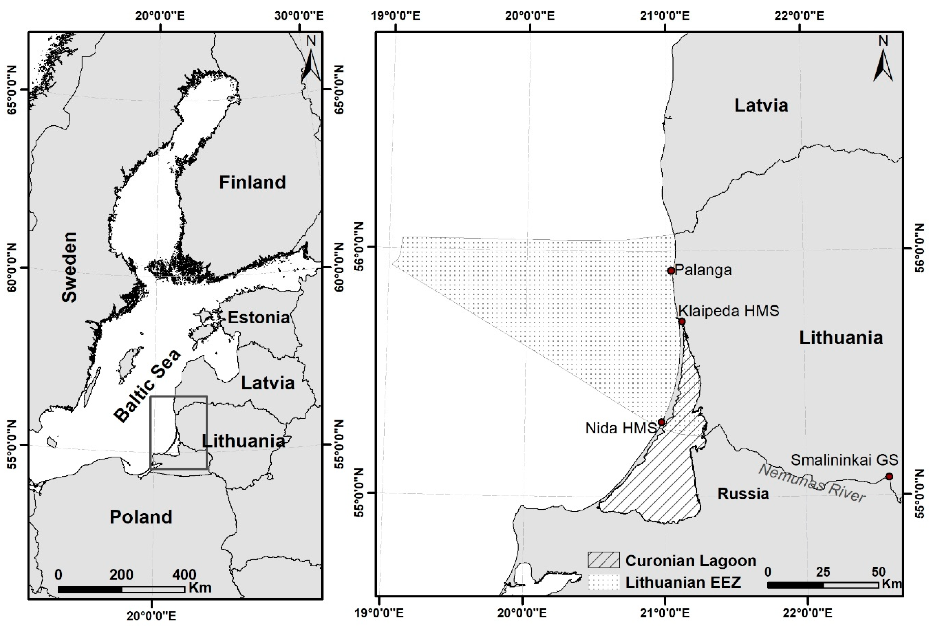
2.1. Study Site

Our study site was comprised of two subareas—the Lithuanian coastal area of the SE Baltic Sea and the Curonian Lagoon (Figure 1). The relatively straight coastline of the SE Baltic Sea is oriented such that coastal upwellings are rather frequently observed in the region under northerly and north-easterly winds [18,26,32]. Apart from the episodic formation of upwelling fronts, the Curonian Lagoon coastal plume, containing highly productive lagoon waters, is another common dynamic feature along the Lithuanian coast [28,33]. On the other hand, there are also cases when the opposite situation occurs, and the inflow of marine waters influences the northern part of the Lagoon.

The Curonian Lagoon itself is the largest (1584 km²) lagoon in the Baltic Sea. It is a relatively shallow (with a mean depth of 3.8 m), highly eutrophied, and predominantly freshwater basin, separated from the open sea by the sandy Curonian Spit. It connects to the Sea through the narrow (0.4–1.1 km) Klaipeda Strait in the northern part of the lagoon. The northern part of the lagoon is a transitory riverine-like system [34] with an active interaction with the Baltic Sea. The annual mean water salinity of 2.45 g kg⁻¹ in the northern Curonian Lagoon can fluctuate up to as high as 7 g kg⁻¹ due to the intrusion of Baltic water [35]. In general, biological diversity is higher in the Curonian Lagoon than in the open coastal waters of the Baltic Sea [36]. The lagoon is dominated by the freshwater phytoplankton species that generally follow a pattern typical of eutrophic ecosystems [37,38]. Marine species only enter the lagoon during seawater intrusions, and the overall abundance of phytoplankton is observed to decrease markedly with increasing salinity [38]. More importantly, the inflow of upwelling waters can supply large amounts of dissolved nutrients to the Curonian Lagoon and change its biotic and abiotic conditions, thus having a significant effect on the changes in Chl-a/primary production.

2.2. Data

In our study, we performed a joint analysis of infrared MODIS data from Aqua/Terra satellites and optical MERIS data installed on the Envisat mission to investigate coastal upwelling events that took place in the Baltic Sea in the period of 2003-2011. The study period was limited by the lifespan of the Envisat mission, which ended in April 2012.

MODIS Sea Surface Temperature (SST) infrared (IR) imagery has been widely used for SST studies in the Baltic Sea (e.g., [18,39,40,41,42]), and the validation of MODIS SST product against in situ observations in the SE Baltic Sea and the Curonian Lagoon has demonstrated a good agreement [28]. Therefore, in this study we used Terra/Aqua MODIS standard Level 2 SST products with a spatial resolution of around 1 km [43]—obtained from the NASA OceanColor website [44]—to analyse upwelling induced surface thermal signatures on the SE coast of the Baltic Sea and in the Curonian Lagoon. The MODIS IR SST Algorithm is detailed in the literature [43]. SST images were processed using the ESA BEAM and ArcGIS software. Following the methodology of previous researches [25,45], a 2 °C threshold (a temperature drop of ≥2 °C relative to ambient waters) was used to distinguish upwelling affected areas from reference zones, and to further analyse the impact of upwelling on Chl-a variability.

For the analysis of the impact of coastal upwelling on the spatial distribution of Chl-a concentration during upwelling events, MERIS/Envisat full-resolution (300 m) cloud-free images were used. Level 1b images were first corrected to account for the difference between the actual and nominal wavelengths of the solar irradiance in each channel [46] with the Smile tool (version 1.2.101) of the BEAM VISAT (4.8.1) software, provided by Brockmann Consult/ESA, in order to perform an irradiance correction for all bands. Chl-a concentration in the coastal waters of the Baltic Sea was retrieved after the application of the FUB processor (version 1.2.4), which was developed by the German Institute for Coastal Research (GKSS), Brockmann Consult, and Freie Universität Berlin. The FUB processor is designed for European coastal waters, and uses MERIS Level 1b top-of-atmosphere radiances to retrieve the concentrations of the optical water constituents [47]. More details on its performance and validation in the study site can be found in the literature [33]. The Chl-a concentration in the Curonian Lagoon was assessed from MERIS data by utilising the semi-empirical band-ratio algorithm (Equation (1)), which uses a reflectance peak in the red and NIR spectral regions [48]. Prior to this, MERIS data was atmospherically corrected by using the Simulation of the Satellite Signal in the Solar Spectrum (6S) code [49]. These algorithms have already been shown to provide accurate estimates via comparison with in situ data collected in the Curonian Lagoon [50,51,52].

$$Chl-a, mg m^{-3}=52.19\times \left(\frac{Re{f}_{708}}{Re{f}_{665}}\right)-32.07$$

(1)

where Ref_x indicates the reflectance of the band with central wavelength x.

Daily mean solar surface incoming shortwave radiation data with a spatial resolution of 0.05 × 0.05 degrees, derived from the satellite-observations of MVIRI/SEVIRI on METEOSAT, were used for the analysis of Chl-a variability. More details on the characteristics of this product are available from the Surface Radiation Data Set—Heliosat (SARAH)—Edition 2 [53].

Three-hourly wind speed and direction data from Klaipeda coastal monitoring station and the daily Nemunas River discharge from Smalininkai gauging station were provided by the Lithuanian Hydrometeorological Service under the Ministry of Environment of the Republic of Lithuania.

2.3. Data Analysis

The phytoplankton responses to the upwelling events along the SE Baltic coast were analysed in terms of changes in Chl-a concentration in relation to changes in SST. 27 upwelling days within 11 distinct upwelling events that had concurrent cloud-free SST and Chl-a maps were analysed in total. Descriptive statistics (means, medians, minimum and maximum values, and standard deviations) were used to represent the estimated parameters and their variability. To reveal whether the changes in Chl-a concentration induced by the upwelling were significant, 30 points were selected specifically for each upwelling case in a way to represent Chl-a concentration in the upwelling and in the reference zone (Figure 2).

Chl-a and SST values individually for each event were extracted at the same locations. The data were tested for normality and met the normality conditions, and therefore no transformations were applied. Statistical comparison between the two groups (Chl-a concentration in the upwelling zone and in the reference zone) was performed after the application of the Welch t-test, which is used to estimate the statistical significance of differences between two groups of samples with possibly unequal variances [54] using R 3.5.1 software.

We examined a set of parameters that might influence Chl-a variability in the SEB coast, including the discharge of the Nemunas River, upwelling-induced SST drop (ΔT), SST inside the upwelling front (hereinafter, upwelling SST), solar radiation, and mean wind speed and direction. Prior to these analyses, a Pearson’s correlation analysis was conducted to test for correlations among quantified environmental parameters. This revealed a strong positive correlation between upwelling SST and ΔT (r = 0.73), and ΔT was therefore excluded from subsequent analyses to eliminate interference from multi-collinearity [55]. To obtain a stressor-response model the nonlinear regression analysis (Generalized Additive Model (GAM)) was applied to the Chl-a data to reveal the influences of the aforementioned environmental factors on the distribution patterns of the Chl-a concentration. The dependent variable was the median value of the Chl-a concentration. The median value was chosen as it is less distorted by outliers [56]. GAM analysis was performed using the Brodgar software, version 2.7.5.

According to the European Union Water Framework Directive 2000/60/EC (EU WFD), all member states are required to protect existing water bodies from deterioration to achieve a “good water status”. For surface waters, the assessment of this status is based on a measurement scale that rates the biological and hydromorphological characteristics of the water by placing them into one of five classes: high, good, moderate, poor, or bad, whereas the chemical characteristics are assessed only as either “good” or “fail” [57]. The values of the boundaries between classes differ among different water bodies based on their physical and hydrographic characteristics. The waters of the Baltic Sea and the Curonian Lagoon have very different hydrophysical and hydrobiological conditions, and therefore the SE Baltic falls under the category of “coastal waters” while the Curonian Lagoon falls under the category of “transitional waters”. Based on the classes of the EU WFD Water quality, the values of Chl-a concentration in the coastal waters of the Baltic Sea and the Curonian Lagoon were classified into the five classes from “high” to “bad”. In addition, reference conditions representing “excellent” status were also indicated. The threshold values of Chl-a concentration used in this work are indicated in

Table 1. Water classes for the warm summer season (June–September) according to WFD.

WFD Classes	Chl-a in the Coastal Waters of the SE Baltic Sea, mg m−3	Chl-a in the Curonian Lagoon, mg m−3
Excellent (reference conditions)	<2.0	<26.4
High	2.0–2.4	26.5–31.7
Good	2.5–4.8	31.8–46.6
Moderate	4.9–7.1	46.7–67.0
Poor	7.2–9.5	67.1–91.9
Bad	>9.5	>91.9

.

3. Results

The analysis of remotely sensed SST and Chl-a data allowed for the identification of upwelling-induced changes along the SEB coast and in the Curonian Lagoon. In this Section, we analyse upwelling-induced Chl-a changes in the coastal zone of the SE Baltic Sea (Section 3.1) and the influence of environmental factors on the Chl-a concentration (Section 3.2), followed by a detailed case study of one upwelling event in the summer of 2008 (Section 3.3). In Section 3.4, we analyse the impact of the upwelled water inflows to the Curonian Lagoon on the spatial distribution of Chl-a concentration in the lagoon.

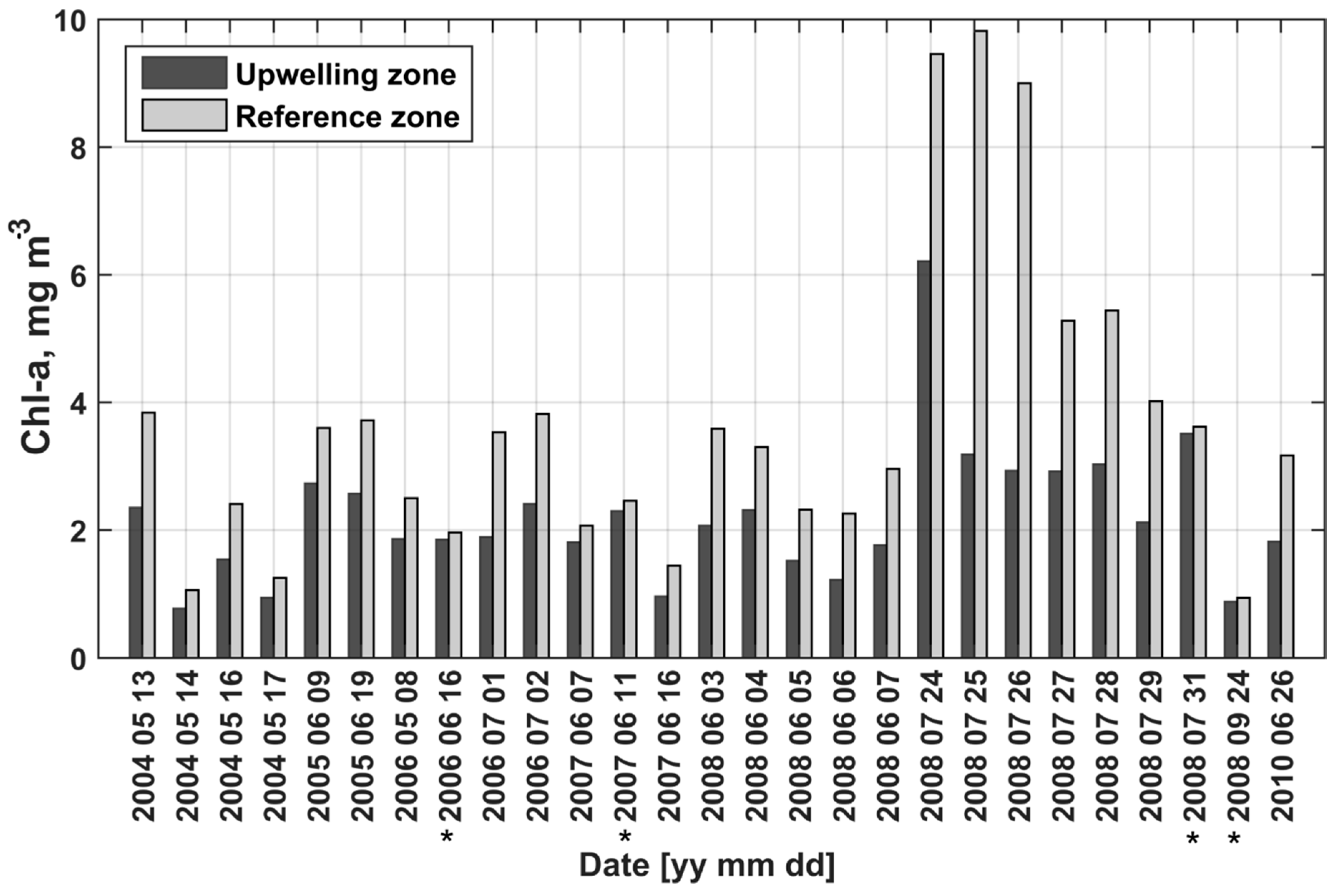
3.1. The Spatio-Temporal Variability of Chl-a Concentration in the Coastal Zone of the SE Baltic Sea

The main characteristics of both remotely sensed SST and Chl-a concentration during upwelling events are presented in

Table 2. Descriptive statistics (mean ± standard deviation) and results of statistical comparison (Welch t–test) of Chl-a and SST in the upwelling and reference zones.

Upwelling Duration	Date	Upwelling Zone		Reference Zone		Upwelling Zone		Reference Zone		t Value	Df
yy mm dd	mm dd	SST, °C		SST, °C		Chl-a, mg m−3		Chl-a, mg m−3
2004 05 12–17	05 13	4.85	±0.75	9.68	±0.59	2.51	±0.96	3.93	±1.09	11.21	38.97
	05 14	4.16	±0.71	9.35	±0.56	0.69	±0.66	1.26	±0.40	6.86	35.79
	05 16	5.56	±0.69	9.34	±0.49	1.66	±0.79	2.50	±0.73	11.05	55.57
	05 17	7.98	±0.21	13.13	±0.87	1.12	±0.76	2.00	±2.44	3.65	51.23
2005 06 09–10	06 09	8.59	±1.32	13.36	±0.43	3.26	±1.59	4.08	±1.35	3.95	52.07
2005 06 18–21	06 19	11.10	±0.96	15.82	±0.35	2.62	±0.88	4.64	±2.74	3.14	47.65
2006 05 07–11	05 08	6.56	±0.67	8.46	±0.38	1.98	±0.59	2.70	±1.00	5.06	31.55
2006 06 14–17	06 16	11.52	±1.06	15.37	±0.56	1.88	±0.42	2.03	±0.46	0.15	54.60 *
2006 07 01–03	07 01	17.40	±0.54	20.94	±0.34	2.08	±0.57	3.61	±0.58	15.80	49.53
	07 02	17.01	±0.88	21.04	±0.48	2.52	±0.83	4.05	±1.12	8.99	49.13
2007 06 07–17	06 07	14.96	±1.24	18.70	±0.45	1.90	±0.94	2.17	±0.62	4.03	52.08
	06 11	14.83	±1.52	20.03	±0.40	2.39	±0.76	2.76	±1.29	1.91	41.40 *
	06 16	12.41	±1.83	18.04	±0.39	1.15	±0.50	1.50	±0.44	3.30	47.30
2008 05 19 / 2008 06 10	06 03	10.66	±1.34	14.86	±0.48	2.25	±0.83	3.88	±1.32	6.32	42.00
	06 04	9.26	±1.20	14.23	±0.59	2.41	±0.82	3.60	±1.41	4.83	40.06
	06 05	9.71	±0.74	14.77	±0.63	1.86	±1.04	2.62	±1.22	2.46	42.13
	06 06	11.91	±0.62	18.68	±1.09	1.26	±0.43	2.29	±0.58	6.25	45.96
	06 07	12.26	±1.20	17.16	±0.56	1.82	±0.67	3.16	±0.97	6.16	52.92
2008 07 25 / 2008 08 03	07 24	18.64	±0.36	19.93	±0.18	7.09	±3.07	10.28	±3.17	14.41	39.13
	07 25	18.70	±0.32	20.19	±0.24	4.10	±1.79	10.51	±3.33	15.44	32.07
	07 26	18.85	±0.34	20.40	±0.19	5.01	±3.71	10.25	±5.56	9.44	30.32
	07 27	18.55	±0.36	20.48	±0.17	3.04	±1.4	5.46	±1.24	9.09	56.61
	07 28	17.72	±0.61	20.45	±0.17	3.08	±0.70	5.54	±1.27	8.16	42.07
	07 29	17.06	±0.09	20.29	±0.14	2.78	±1.95	4.31	±1.56	5.49	50.54
	07 31	17.84	±0.76	20.44	±0.15	3.66	±0.98	3.82	±1.19	1.51	42.25 *
2008 09 23–26	09 24	10.32	±0.91	15.78	±0.44	1.03	±0.36	0.94	±0.34	1.05	56.59 *
2010 06 22–29	06 26	12.27	±0.67	14.99	±0.30	1.95	±0.68	3.51	±1.54	3.65	40.67

Date is the day when satellite measurements were performed. Df is the Degrees of Freedom; *asterisk indicates statistically insignificant differences.

. As can be seen, the temperature difference in the upwelling zone compared to the ambient waters varied from 2 °C to 9 °C (with a median of 5.43 °C). During some events, the upwelling-induced SST values were very low and atypical for the given months. For example, SST values observed during the upwelling event in May 2004 dropped down to as low as 3–4 °C, and were more similar to SSTs usually observed in March (2–4 °C on average) than in May (10–12 °C on average) (see e.g., [28]). During summer months, the upwelling-induced SST values dropped down below 10 °C, thus significantly altering the abiotic conditions of the study area.

In addition to the SST changes, this analysis shows that significant changes in Chl-a concentration were recorded during upwelling events, with a clear reduction in the latter in the upwelling affected zone compared to the reference (ambient) waters. Mean Chl-a concentration in the upwelling zone varied from 0.69 to 7.09 mg m⁻³ across different upwelling events, while in the reference zone the mean concentration was higher and varied from 1.26 to 10.51 mg m⁻³. The statistical comparison of mean and median Chl-a concentrations reveals that in 89% of the cases analysed, the difference in Chl-a concentration between the upwelling and the reference zones is significant, and was usually around 40–50% lower in the upwelling zone than in the ambient waters (Table 2, Figure 3).

The differences in Chl-a concentration that were insignificant could, to a certain extent, be explained by the phase of upwelling during which the Chl-a values were observed (Table 2, Figure 3). For example, the Chl-a concentration values from 16 July 2006 and 31 July 2008 were measured during the upwelling relaxation phase, thus the gradual increase in SST was accompanied by a slight increase in Chl-a, causing the Chl-a concentration in the upwelling zone to become similar to the one observed in the ambient waters. On the other hand, upwelling was still in the active phase on 11 June 2006 and 24 September 2008, when the difference in Chl-a concentration between the upwelling and the reference zones was insignificant, suggesting that other environmental variables influencing Chl-a variability also have to be considered.

This analysis also shows that the distribution patterns of Chl-a concentration in the upwelling zone might differ due to strong event-scale variability and prevailing environmental conditions (Table 2, Figure 3). For example, the upwelling induced ΔT in June 2008 reached over than 7 °C, while in July 2008 ΔT was smaller at around 3 °C. At the same time, a drop in Chl-a concentration in the upwelling area was recorded in the July event that was up to six times larger than the one in June 2008. The Chl-a decrease in July 2008 was the largest of all of the cases analysed, and therefore special attention will be paid to a detailed analysis of this particular upwelling event in Section 3.3.

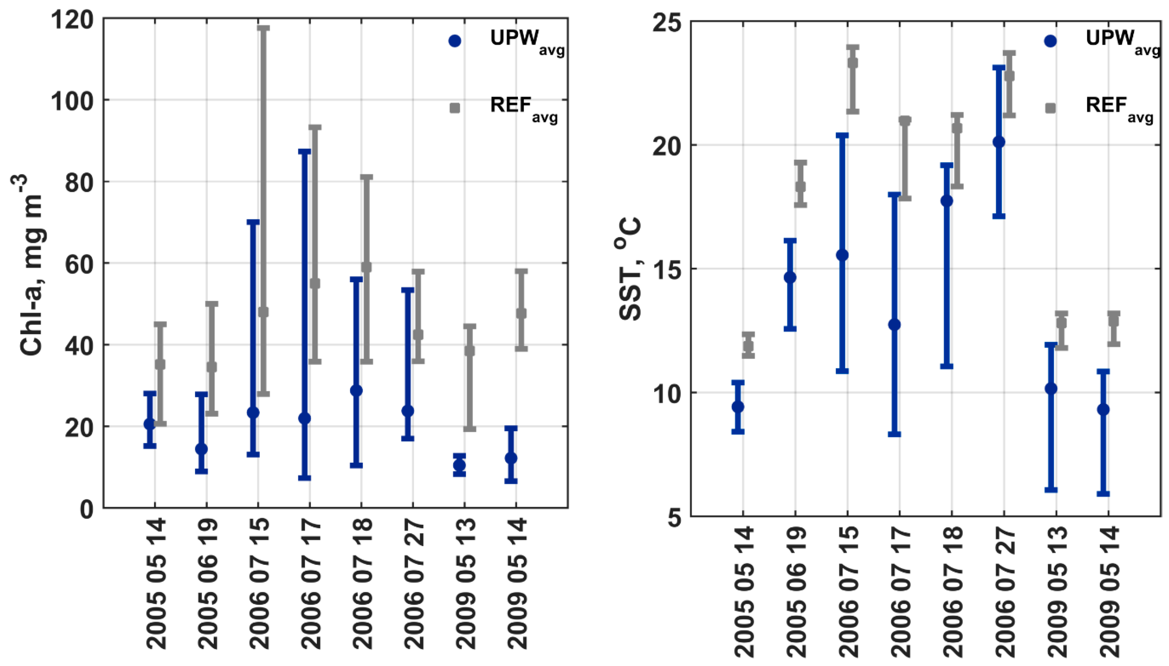
3.2. The Importance of Environmental Factors on the Variation of Chl-a Concentration During Coastal Upwelling

Environmental factors—i.e., upwelling SST, the discharge of the Nemunas River, solar radiation, and wind speed—varied during separate upwelling events, while the prevailing winds were mostly of a northerly direction as they favour the development of upwelling in the SE part of the Baltic Sea. The application of GAM shows that the combination of the five aforementioned environmental variables explains 77.5% of the variation in the Chl-a concentration (

Table 3. Descriptive statistics and relative importance (F value) of the explanatory variables for the observed changes in Chl-a concentration (median value) in the upwelling zone (* significant factors are marked with asterisks).

Environmental Variable n = 22	Mean	Minimum	Maximum	F Value
* Upwelling SST, °C	14.2	8.6	18.9	3.45
* Solar radiation, W m−2	311	141	349	2.83
* Wind speed, m s−1	4.3	2	7.8	1.92
Nemunas river discharge, m3 s−1	400	268	735	0.23
Wind direction	predominant N-NW winds			0.36
Deviance explained				77.50%

).

The GAM also shows upwelling SST to be the most important variable, followed by solar radiation and wind speed, in explaining Chl-a variations in the upwelling zone. SST inside the upwelling front varied from 8.6 to 18.9 °C, and a positive relationship was determined between upwelling SST and Chl-a concentration in that a decrease in SST is usually associated with a decrease in Chl-a. Higher values of solar radiation were also associated with higher Chl-a concentrations. Wind speed was around 4 m s⁻¹ on average, although several cases of wind speeds exceeding 6 m s⁻¹ were observed (Table 3). The relationship between Chl-a concentration and wind speed showed that higher Chl-a values were observed under lower wind speeds. The wind direction and the discharge of the Nemunas River did not exhibit any significant impact on Chl-a values.

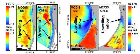
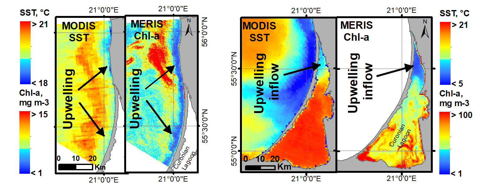
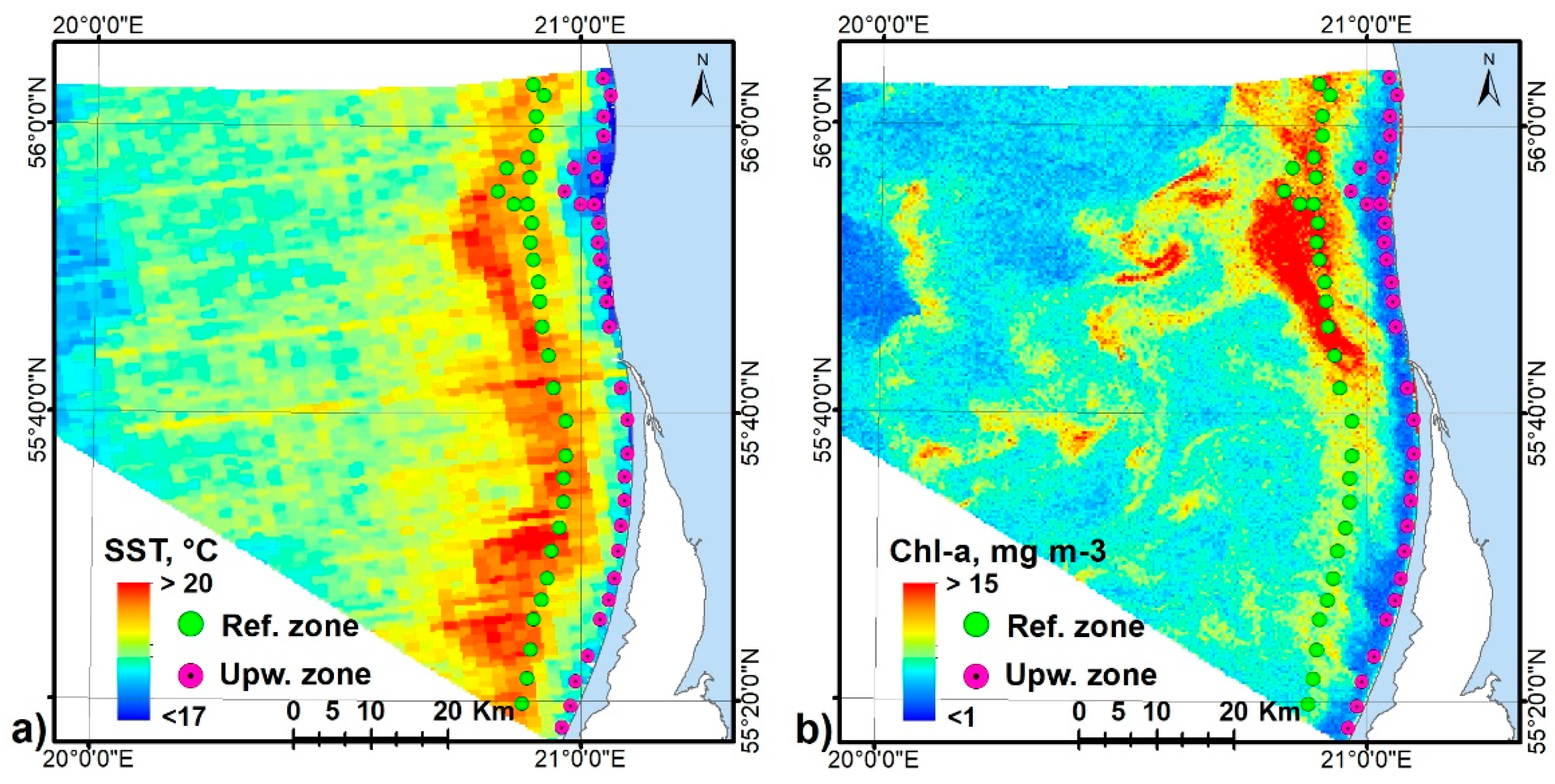
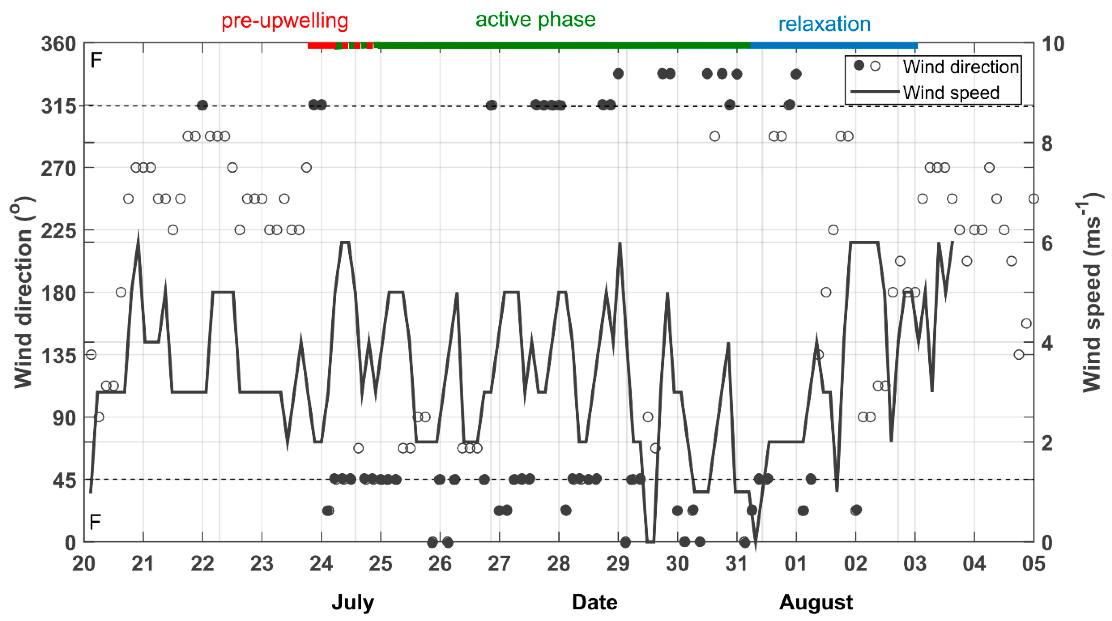
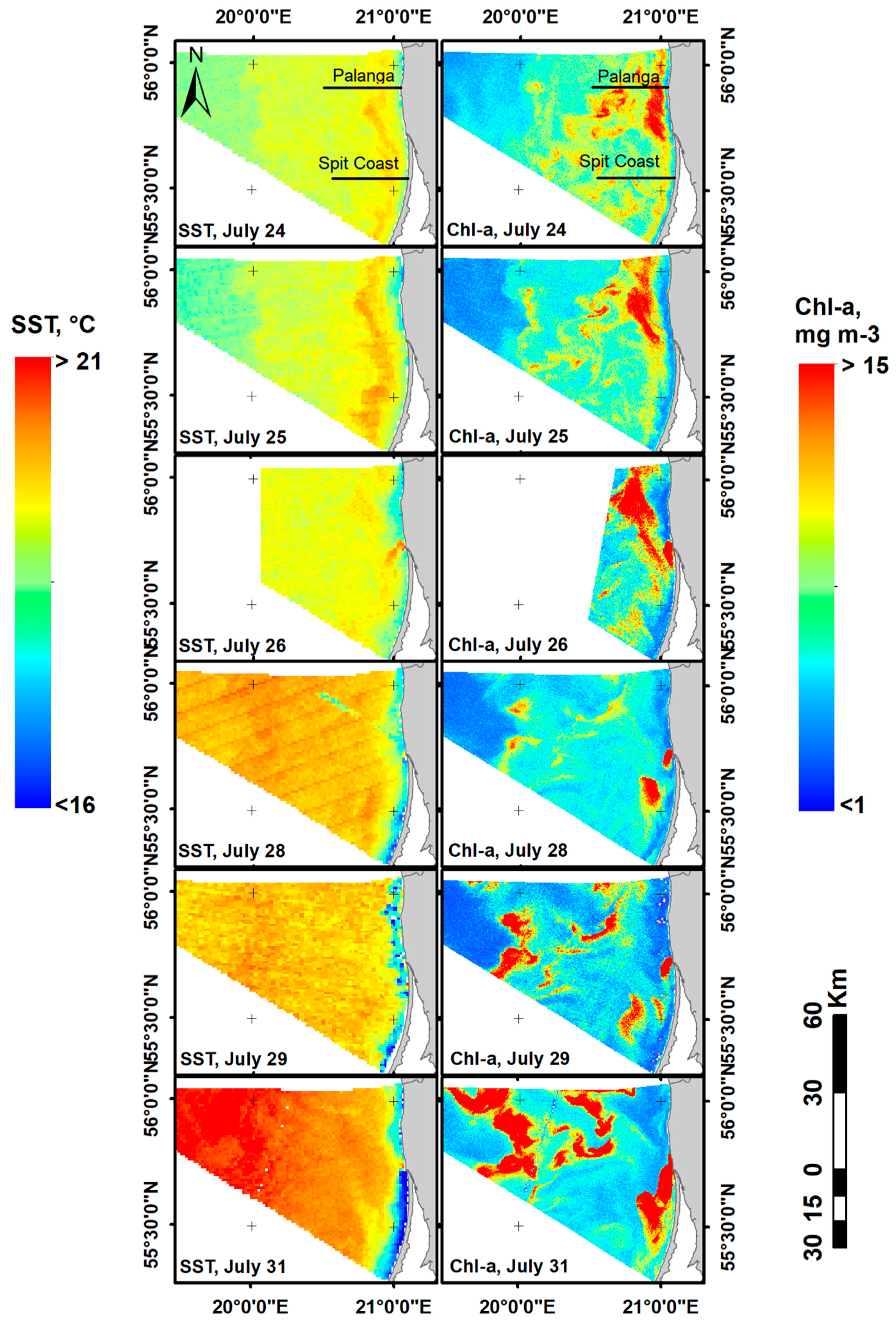
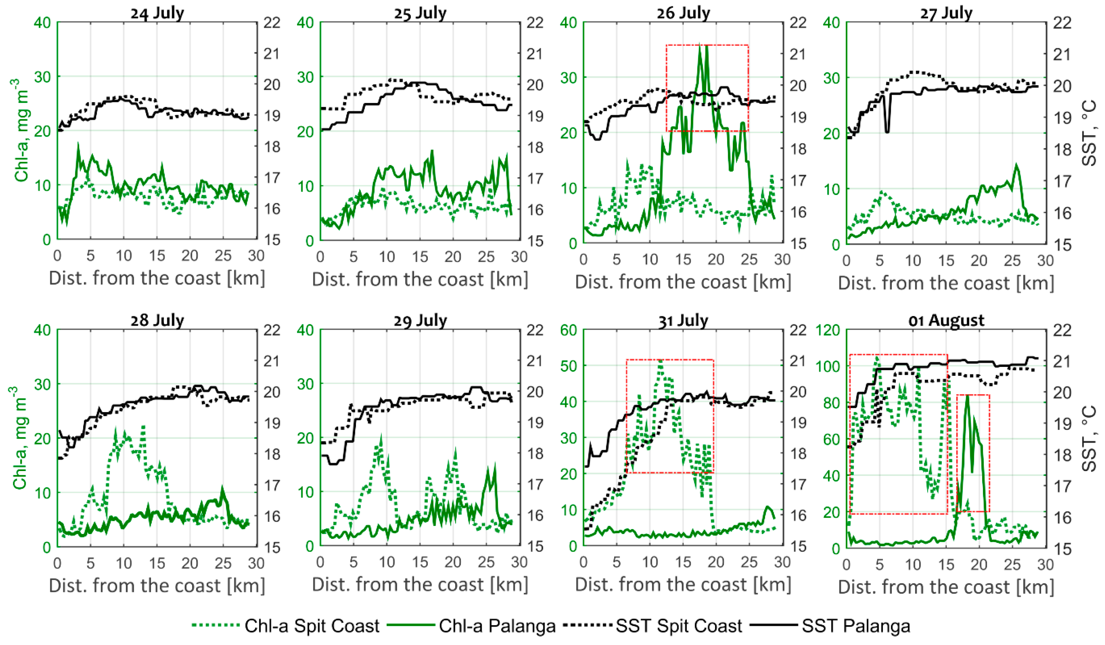
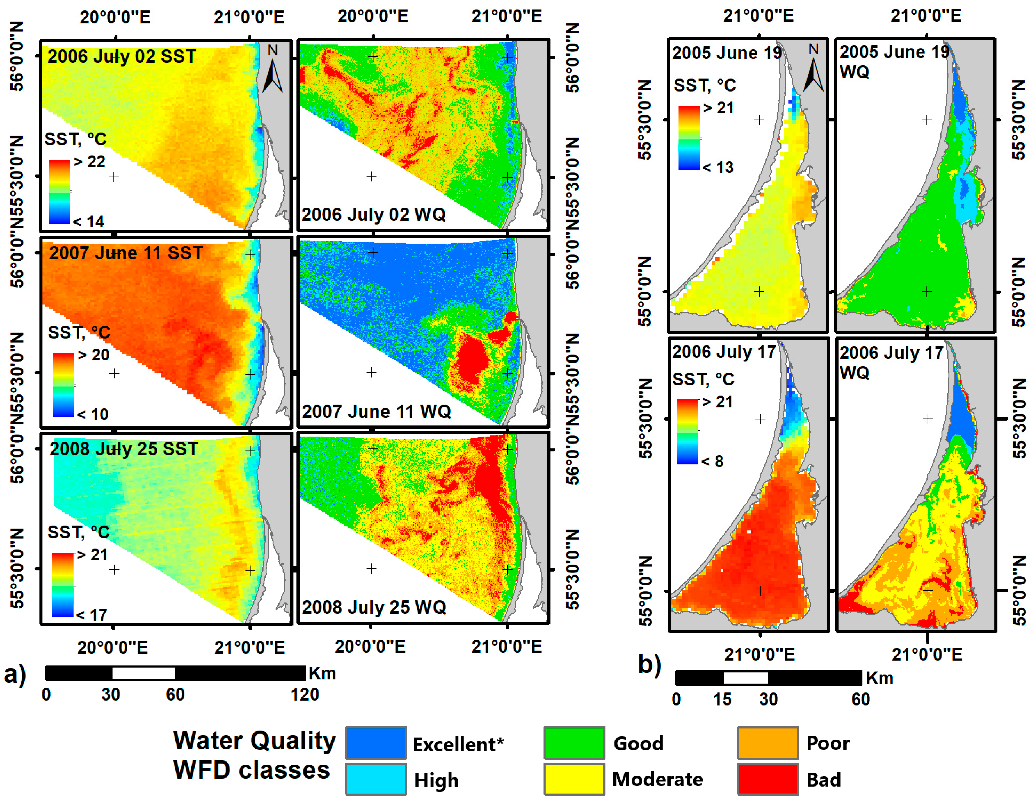
3.3. A Detailed Case Study of the Upwelling event in the Summer of 2008

The upwelling event that occurred in the period of July–August 2008 was chosen for more detailed consideration as there were a substantial number of sequential satellite SST and Chl-a images available, and this event was characterised by the largest drop in Chl-a concentration among the all cases analysed. Using satellite data, the relatively cold and low-chlorophyll surface waters along the coast can be clearly distinguished in summertime from the warm and chlorophyll-rich offshore waters. The meteorological situation at the time of the development of this upwelling is presented in Figure 4. The evolution of this upwelling event, characterised by pronounced changes in the near-shore SST and Chl-a distributions, is illustrated in Figure 5 and Figure 6.

Wind field measurements from the Klaipeda hydrometeorological station (see Figure 1) show that variable wind conditions prevailed at the end of July and at the beginning of August. From this record, the phases in the development of the upwelling could be distinguished (Figure 4). As seen in the data, the upwelling was apparently triggered by persistent upwelling-favourable northerly winds of 3–6 m s⁻¹, with a relatively short pre-upwelling phase lasting from the end of July 23 to July 24.

The active phase, during which an offshore Ekman transport of surface waters was induced, was observed starting from July 24–25. Some variations in the wind direction occurred on July 25–26; yet, upwelling-favouring winds were most intense during this period. In general, northerly winds were dominant until July 31, particularly favouring the development of upwelling from July 27 until the end of the month. After July 31, the wind direction changed and the upwelling entered the relaxation phase, although the offshore spreading of its front at the sea surface was observed until around August 3.

The satellite SST maps indicated the response of the surface waters to the upwelling-favouring winds, starting from July 24. Although the water masses near the coast became slightly colder than the open sea (ΔT = 1.67 °C), the temperature difference was too small yet to clearly define the upwelling event from the SST record if the 2 °C threshold was applied. On the contrary, the signatures of upwelling were well depicted in the Chl-a map of the same day (July 24), when more productive coastal waters were transported further offshore, so marking the beginning of the upwelling event (Figure 5 and Figure 6).

Despite SST records indicating the beginning of the upwelling event a day later, the Ekman offshore drift depicted in the Chl-a records implies that the pre-upwelling phase lasted until 24 July. This is well seen from the horizontal Chl-a profiles near the Curonian Spit and, especially, near Palanga, where a northward plume of highly productive Curonian Lagoon waters was observed prior to the upwelling event. When northerly winds became dominant, the spatial orientation of the plume changed drastically: the plume waters were separated from the coast due to upwelling-induced offshore transport. In turn, a sharp difference in Chl-a concentration within the first 2 km of water from the coast (3–5 mg m⁻³) compared to the waters further from the coast (up to 17 mg m⁻³) was observed near Palanga. The Chl-a decrease along the coast of the Curonian Spit was slightly smaller, from 9 mg m⁻³ observed offshore down to around 5–7 mg m⁻³ along the coast (Figure 6).

On July 25, the upwelling signatures became more distinct: SST maps showed ΔT reaching approximately 2 °C; and Chl-a maps depicted the upwelling zone as a wide (>5 km) band of low Chl-a concentration along the coast (Figure 6). As retrieved from satellite images, a clear reduction in Chl-a concentration (~4 mg m⁻³) was observed across the entire coastal zone relative to the ambient waters unaffected by upwelling (up to 15 mg m⁻³ near Palanga and ~8 mg m⁻³ near the Curonian Spit). On July 26, the hydro-biological situation became more complex in the coastal zone near the entrance to the lagoon, because the southward outflow of fresh, warm, and highly productive waters from the lagoon divided the upwelling zone into northern and southern parts (Figure 5). The Chl-a profile of July 26 showed a very distinct drop in Chl-a concentration near Palanga, down to about 2–5 mg m⁻³ in the first 10 km of water adjacent to the coast—values up to five times smaller than those observed further from the coast (20–35 mg m⁻³). At the same time, the Chl-a rich waters continued moving further south.

In the period of July 27–31 the upwelling-favourable wind conditions continued, and the strongest development of the upwelling front occurred, making it very distinct in the SST records (ΔT up to 5 °C). The more mature the upwelling became, the more severe was the drop observed in Chl-a concentration in coastal waters, with the lowest values (~3 mg m⁻³) recorded on July 27–29. At the same time, the Curonian Lagoon plume became very intense (Figure 5), and a clear trail of more productive waters (Chl-a concentration up to 50 mg m⁻³) steering to the south was evident on July 31. As can be seen from SST maps, the upwelling front was more pronounced to the south of the Klaipeda Strait than in the northern area, where it separated highly productive plume waters from the coast.

From the beginning of the upwelling (July 24) to the onset of its relaxation (after July 31), the mean values of Chl-a concentration in the coastal waters decreased steadily from around 7 mg m⁻³ to less than 3 mg m⁻³, and only when the upwelling fully entered its relaxation phase did they begin to increase slightly—as the horizontal Chl-a profile of August 01 indicates (Figure 6).

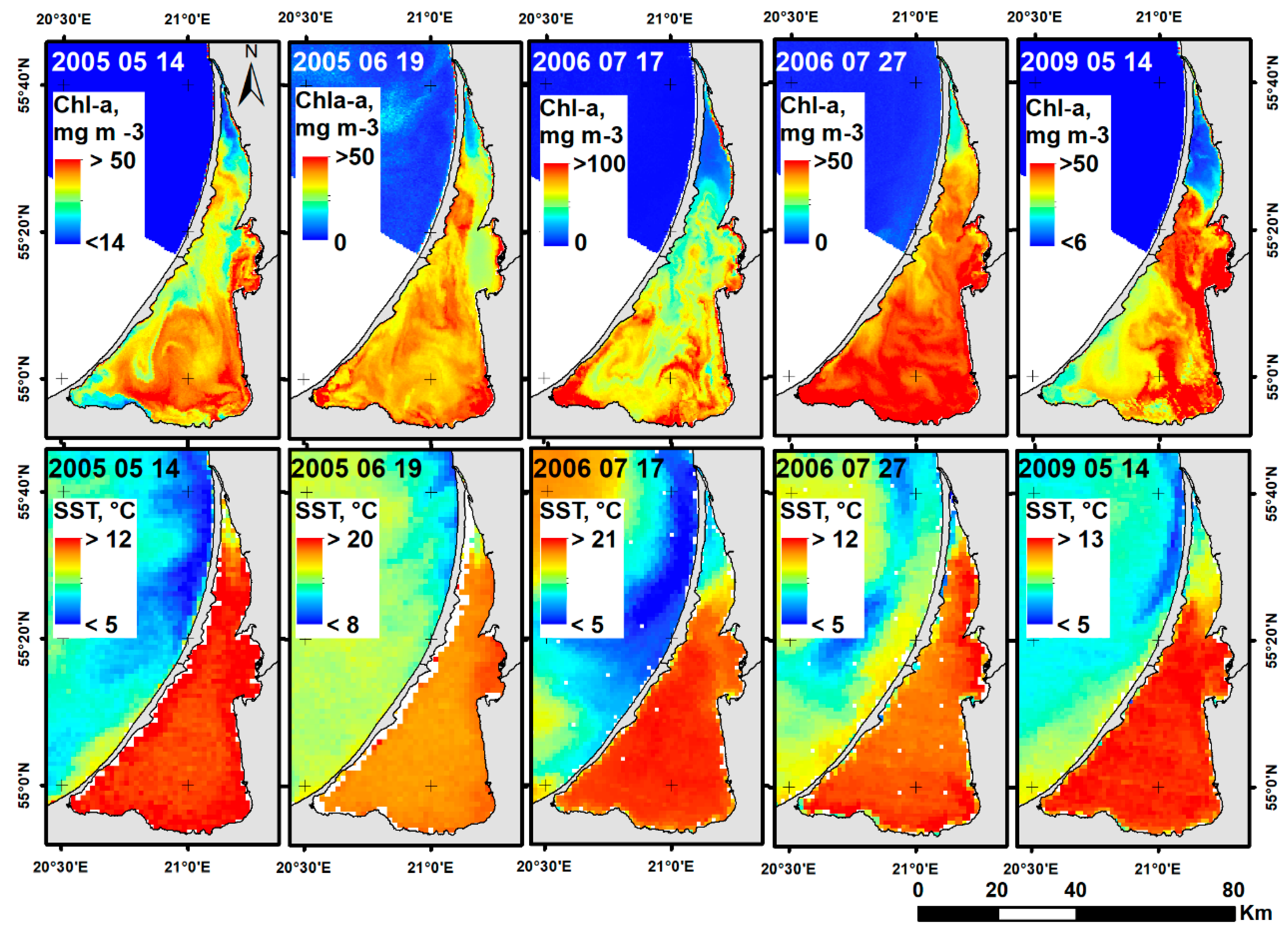
3.4. The Influence of Upwelling on the Chl-a Concentration of the Curonian Lagoon

The analysis of satellite data showed that the existence of upwelling fronts along the SEB coast was often accompanied by a freshwater plume from the Curonian Lagoon. However, there were also cases when the opposite situation occurred, and inflows of marine waters during upwelling events that influenced water masses in the northern part of the lagoon were recorded. To address this in more detail, cases with concurrent SST and Chl-a maps were analysed in order to document the spatial scales of upwelling inflows and their impact on horizontal SST and Chl-a distributions in the lagoon (Figure 7).

As retrieved from satellite images (Figure 7), inflows of upwelling waters reached the middle part of the lagoon fairly often, with a propagation distance of up to 30 km southward—as recorded in July 2006 and May 2009, for example. During such events, relatively cold marine waters low in Chl-a pushed away and diluted the highly productive waters of the northern Curonian Lagoon. Although SST and Chl-a concentrations in the lagoon varied greatly across different months, the upwelling-induced changes in both parameters were higher in the lagoon than along the SEB coast. The average upwelling-induced SST drop in the lagoon was approximately 5–7 °C, reaching up to ~16 °C during a very intensive upwelling in July 2006. The horizontal changes in Chl-a concentration were even more pronounced, dropping down by an order of magnitude during the same event.

Figure 8 shows the SST and Chl-a changes observed in the Curonian Lagoon during the selected coastal upwelling events from 2005 to 2009. First, we will consider that typical values of these parameters were observed in the ambient waters throughout the season. As seen, the smallest SST values were observed in May, with an average value of around 12 °C. Throughout the summer season, the SST increases to 18 °C in June and to 24 °C in July. In May and June, the Chl-a concentration was approximately 35–50 mg m⁻³ on average, with maximum values reaching 65 mg m⁻³. In July, the average concentration was even higher at around 50–60 mg m⁻³, reaching up to 120 mg m⁻³. This corresponds well to the Chl-a values typically observed in the Curonian Lagoon, as the mean climatological concentration of Chl-a is 47.6 ± 15.7 in May, 43.2 ± 29.41 in June, and 71.9 ± 51.3 mg m⁻³ in July [58]. However, during upwelling inflows both of these properties decreased severely in the areas affected—2–8 °C in SST and 2–4 orders of magnitude in Chl-a concentration.

In particular, the Chl-a concentration and water temperature of the Curonian Lagoon were strongly affected by a major upwelling event that took place in July 2006. Here, a sharp drop in SST from 21 °C to 8 °C (ΔT = 12.7 °C on average) was recorded in the upwelling inflow area, which was much lower compared to those SST recorded in the reference area (minimum SST 17.8 °C, average SST 21 °C). In addition, this particular upwelling inflow resulted in the Chl-a concentration to drop down to several mg m⁻³ while in the reference area it remained above 100 mg m⁻³. Another upwelling inflow event in May 2009 demonstrated that in some cases upwelling can result in only a slight SST drop, but can at the same time lead to a pronounced decrease in Chl-a concentration. For this particular event, the upwelling induced temperature drop was only 2–4 °C, but the average Chl-a concentration in the inflow zone (10–12 mg m⁻³) was nearly 4 times lower than in the ambient waters (40–50 mg m⁻³).

4. Discussion

Environmental parameters such as water transparency, SST, salinity, and nutrient availability are subjected to high variability due to coastal upwelling in the Baltic Sea [18,24,59,60,61], which is also recognized as an efficient contributor to the exchange processes between coastal and offshore waters [62]. In turn, upwelling events that take place during the warm season may have an important influence not only on coastal SST patterns and vertical stratification, but also on the entire coastal environment through their effect on biological processes [63].

SST, in general, is one of the primary indicators of upwelling during the warm season in the Baltic Sea, and it is not ordinarily possible to recognize the beginning of an upwelling from SST maps when cooler water has been uplifted but has not yet surfaced [42]. Despite this, a detailed study of the upwelling event of July 2008 has revealed that the development of an upwelling event can be identified in Chl-a maps before thermal signatures in the surface layer appear. In this case, a significant increase in water transparency marked the beginning of the coastal upwelling in the Chl-a records. The decline in Chl-a concentration during upwelling events is due to the lateral displacement of water masses, when the peak of Chl-a production is physically removed from the upwelling region due to cross-frontal advection [60,64], and only later do temperature changes come about.

The application of the GAM model to better understand the role of various abiotic factors on Chl-a changes during upwelling events has shown that the SST of the upwelling zone (or the SST drop between ambient and upwelling waters) is the most influential variable (see Table 3), in that lower temperatures in the upwelling zone are associated with lower Chl-a concentrations. This could either be related to the displacement of water masses and the transport of more productive waters further offshore [22,60,64], or to the decrease in water temperature—which is unfavourable for the production of phytoplankton [21]. The GAM also shows that the increase in solar radiation positively affects the development of Chl-a, which is the key variable affecting the growth of phytoplankton [16,65,66]. The increase in solar radiation is also directly linked to the rise of SST, which favours the proliferation of phytoplankton biomass. As further outlined, wind speed has a significant influence on Chl-a distribution patterns as wind-induced mixing largely determines the distribution of phytoplankton in the upper layer, decreasing the surface Chl-a concentration by mixing phytoplankton deeper into the water column [67]. Higher Chl-a values were, therefore, observed under lower wind speeds. Overall, the application of the GAM shows that the environmental variables analysed explain 77.5% of the observed deviance in Chl-a concentration, implying that other factors—such as vertical nutrient flux—should be taken into account when evaluating the impact of upwelling events on the functioning of a coastal ecosystem.

The analysis of cloud-free MODIS and MERIS/Envisat images evidently revealed the effect of upwelling on significantly lowering the SST and the Chl-a concentrations not only along the SE coast of the Baltic Sea but also in the Curonian Lagoon. In the lagoon, the background SST and Chl-a concentrations were much higher than in the sea, leading to more severe SST and Chl-a drops caused by the inflow of upwelled water. Such short-term marine inflow events could be very rapid and even reach the southern part of the Curonian Lagoon [28,29], altering the temperature and salinity patterns therein. Such inflows might also have a longer-term impact on the growth of phytoplankton in the Curonian Lagoon, where the supply of nutrients—such as nitrogen or phosphorus—depends on the volume of inputs from the Baltic Sea and terrestrial sources [68]. Moreover, the structural and functional characteristics of phytoplankton communities are also known to differ significantly between ambient regions and marine water inflow areas [69]. We may, therefore, expect coastal upwelling to have a much more severe effect on primary production changes in the Curonian Lagoon than in the Baltic Sea.

Due to the upwelling-induced uplift of deeper water layers to the surface [59], nutrient concentrations in the upper layer can become significantly higher during and after upwelling events [70,71]. Such changes can cause a “random noise” in the time series of phosphate, nitrate, and Chl-a concentrations, potentially masking anthropogenic effects in the status assessments of the Water Framework Directive (WFD) and the Marine Strategy Framework Directive (MSFD) [7]. Coastal upwelling should, therefore, be considered an important dynamic process for the comprehensive assessment and management of water bodies [10]—as was done, e.g., for the Italian seas [72]. Even though it is a natural process, this might create a new challenge: to understand the role of dynamic oceanographic features that affect good environmental status [7], and to learn how to apply this knowledge for the implementation of various directives.

Available satellite data allowed us to investigate the effect of upwelling on water quality. The analysis of the Chl-a and SST images of the SE Baltic Sea region shows that through the reduction in Chl-a concentration, the effect of upwelling could be linked to better water quality in the coastal zone compared to pre-upwelling periods or offshore regions. Several examples showing WFD water quality classes based on Chl-a concentration along the SEB coast and in the Curonian Lagoon are presented in Figure 9. This demonstrates that upwelling-affected waters can be distinguished from ambient ones as having better quality based on the WFD water quality classes.

This is very well exemplified in the upwelling cases of 02 July 2006 and 25 July 2008 (Figure 9a). Here the “excellent” to “good” quality waters along the coast are clearly distinguished from the offshore regions, which have high Chl-a concentrations and “poor” to “bad” water status according to the WFD water quality classes. A similar picture can be observed on 11 June 2007, where a distinct band of “moderate” to “bad” quality waters in the Curonian Lagoon plume are surrounded by “excellent” to “good” quality water in the upwelling region.

It is also worth noting that the Curonian Lagoon is considered to be an important element of the tourism development in the region. However, the eutrophication of the lagoon and poor water quality insufficient for bathing [73], intensive summer algae blooms, and low water transparency all negatively influence the socio-economic development of the region [74]. In this context, it is important to mention the upwelling-induced entrainment of water into the hyper-eutrophic Curonian Lagoon which, as has been already shown, leads to a short-term reduction in Chl-a concentration and the improvement of water quality (Figure 9b). During such events, inflow regions with relatively low temperatures are characterised by “excellent” water quality, whereas ambient waters could be characterised as poorly as “bad” depending on the initial Chl-a concentration in the lagoon. Even though any improvement in water quality would be a short-term event in this case, it can still improve the recreational potential of the region.

This study explored the possibility of determining water quality during upwelling events with remote sensing images from cloud-free MERIS/Envisat images. The results of the study suggest that such events should be taken into account when evaluating the overall state of the environment, as the measurement of water quality indicators during upwelling events might represent very different conditions from typical ones, thus necessitating continuous monitoring. Due to the collapse of MERIS in 2012, the number of available Chl-a images decreased, yet the launch of Sentinel-2 in 2015 and Sentinel-3 in 2016—having two optical instruments, MultiSpectral Instrument (MSI) and Ocean and Land Colour Instrument (OLCI) respectively—increased the number of available Chl-a images significantly [58]. In turn, Sentinel satellites provide a scientific opportunity for the high-frequency monitoring of the water quality of coastal waters, enabling not only operational monitoring but also studies on environmental change [75]. Therefore, they have great potential for the remote sensing of coastal water, and are an important tool for its monitoring and research [76].

However, here we must acknowledge that our water quality estimates are based on Chl-a concentration only, and do not consider changes in the amounts of nutrients (N, P) that are critical for the management of eutrophication [77]. The role of the temporal and spatial limitations of nutrients on phytoplankton growth in developing successful management strategies has been highlighted in the study by authors of [78]. Similarly, EU directives also imply that the monitoring and management of vulnerable coastal ecosystems should follow a holistic approach. Therefore, more complete water quality monitoring requires the integration of in situ measurements with recent developments in techniques such as remote sensing, numerical modelling, and other advanced information technology [10,79]. Hence, the investigation of N and P budgets, trends, variability, and fate caused by coastal upwelling should be addressed in the near future, combining both conventional monitoring and remote sensing methods.

5. Conclusions

This study presents the results of a satellite-based analysis of Chl-a variability in the coastal zone of the SE Baltic Sea and in the Curonian Lagoon during wind-induced coastal upwelling events. Multi-spectral satellite data allowed the authors to quantify the influence of coastal upwelling on the horizontal distribution of SST and Chl-a concentration. Analysis showed that the Chl-a concentration in the upwelling regions of the SE Baltic is, on average, 40–50% lower than in ambient waters.

As observed, the primary cause of the reduction in Chl-a concentration in the coastal zone is related to the lateral offshore transport of warm and productive coastal waters. The first signatures of upwelling could be identified in the Chl-a maps before the thermal signatures even appear in the surface layer, suggesting that these data can be used for the early detection of upwelling events.

The application of the GAM model showed that the local SST inside the upwelling front, wind speed, and solar radiation are the primary factors related to the observed changes in Chl-a. However, a comprehensive assessment of the influence of upwelling on the coastal ecosystem also requires the integration of in situ measurements, providing additional information on nutrient concentrations.

The analysis of satellite data also shows clear evidence of the influence of coastal upwelling on the hydrobiological conditions of the shallow, eutrophied Curonian Lagoon. In particular, strong SST and Chl-a gradients resulting from the inflow of upwelled water were identified in the northern part of the lagoon. As the Curonian Lagoon is a semi-enclosed water body, the corresponding impact of coastal upwelling on its hydrobiological properties—and on the overall ecosystem—is higher than along the SEB coast.

This study also outlines the influence of upwelling on water quality along the SEB coast and in the Curonian Lagoon due to the spatio-temporal variability of the Chl-a concentration across these water bodies. As demonstrated, multi-mission satellite data may be effectively used for monitoring environmental status and water quality in coastal areas, thus demonstrating the practical use of the results obtained and the Earth’s observations in water management. The example of the Baltic Sea has also shown that upwelling events should be taken into account when performing both national, European, and Regional Seas monitoring plans and when evaluating trends in water quality or considering measures for the regulation of ecological status in coastal waters.

References

1. Savchuk, O.P. Large-Scale Nutrient Dynamics in the Baltic Sea, 1970–2016. Front. Mar. Sci. 2018, 5, 5. [Google Scholar] [CrossRef]
2. HELCOM. HELCOM Thematic Assessment of Eutrophication 2011–2016. Baltic Sea Environment Proceedings No.156. 2018. Available online: http://www.helcom.fi/baltic-sea-trends/holistic-assessments/state-of-the-baltic-sea-2018/reports-and-materials/ (accessed on 3 June 2020).
3. HELCOM. The Fourth Baltic Sea Pollution Load Compilation (PLC-4). Baltic Sea Environment Proceedings No. 93. Helsinki Commission; HELCOM: Helsinki, Finland, 2004; 188p. [Google Scholar]
4. Schernewski, G.; Neumann, T. The trophic state of the Baltic Sea a century ago: A model simulation study. J. Mar. Syst. 2005, 53, 109–124. [Google Scholar] [CrossRef]
5. Savchuk, O.P.; Wulff, F.; Hille, S.; Humborg, C.; Pollehne, F. The Baltic Sea a century ago—A reconstruction from model simulations, verified by observations. J. Mar. Syst. 2008, 74, 485–494. [Google Scholar] [CrossRef]
6. HELCOM. Eutrophication in the Baltic Sea—An Integrated Thematic Assessment of Eutrophication in the Baltic Sea Region. Baltic Sea Environmental Proceedings No. 115B. Helsinki Commission; HELCOM: Helsinki, Finland, 2009; 148p. [Google Scholar]
7. Myrberg, K.; Korpinen, S.; Uusitalo, L. Physical oceanography sets the scene for the Marine Strategy Framework Directive implementation in the Baltic Sea. Mar. Policy 2019, 107, 103591. [Google Scholar] [CrossRef]
8. Matarrese, R.; Chiaradia, M.; De Pasquale, V.; Pasquariello, G. Chlorophyll-a concentration measure in coastal waters using MERIS and MODIS data. In Proceedings of the IGARSS’04 2004 IEEE International Geoscience and Remote Sensing Symposium, Anchorage, AL, USA, 20–24 September 2004; Volume 6, pp. 3639–3641. [Google Scholar]
9. Zhang, H.; Qiu, Z.; Sun, D.Y.; Wang, S.; He, Y. Seasonal and Interannual Variability of Satellite-Derived Chlorophyll-a (2000–2012) in the Bohai Sea, China. Remote Sens. 2017, 9, 582. [Google Scholar] [CrossRef] [Green Version]
10. Gholizadeh, M.H.; Melesse, A.M.; Reddi, L. A Comprehensive Review on Water Quality Parameters Estimation Using Remote Sensing Techniques. Sensors 2016, 16, 1298. [Google Scholar] [CrossRef] [Green Version]
11. Spyrakos, E.; Vilas, L.G.; Palenzuela, J.M.T.; Barton, E.D. Remote sensing chlorophyll a of optically complex waters (rias Baixas, NW Spain): Application of a regionally specific chlorophyll a algorithm for MERIS full resolution data during an upwelling cycle. Remote Sens. Environ. 2011, 115, 2471–2485. [Google Scholar] [CrossRef] [Green Version]
12. Nieto, K.; Mélin, F. Variability of chlorophyll-a concentration in the Gulf of Guinea and its relation to physical oceanographic variables. Prog. Oceanogr. 2017, 151, 97–115. [Google Scholar] [CrossRef]
13. Pinochet, A.; Garcés-Vargas, J.; Lara, C.; Olguin, F. Seasonal Variability of Upwelling off Central-Southern Chile. Remote Sens. 2019, 11, 1737. [Google Scholar] [CrossRef] [Green Version]
14. Nômmann, S.; Sildam, J.; Nôges, T.; Kahru, M. Plankton distribution during a coastal upwelling event off Hiiumaa, Baltic Sea: Impact of short-term flow field variability. Cont. Shelf Res. 1991, 11, 95–108. [Google Scholar] [CrossRef]
15. Laanemets, J.; Kononen, K.; Pavelson, J.; Poutanen, E.-L. Vertical location of seasonal nutriclines in the western Gulf of Finland. J. Mar. Syst. 2004, 52, 1–13. [Google Scholar] [CrossRef]
16. Lips, I.; Lips, U. Phytoplankton dynamics affected by the coastal upwelling events in the Gulf of Finland in July-August 2006. J. Plankton Res. 2010, 32, 1269–1282. [Google Scholar] [CrossRef] [Green Version]
17. Kratzer, S.; Ebert, K.; Sørensen, K. Monitoring the Bio-optical State of the Baltic Sea Ecosystem with Remote Sensing and Autonomous In Situ Techniques. In The Baltic Sea Basin; Harff, J., Björck, S., Hoth, P., Eds.; Springer: Berlin/Heidelberg, Germany, 2011; pp. 407–435. ISBN 978-3-642-17220-5. [Google Scholar]
18. Dabuleviciene, T.; Kozlov, I.E.; Vaiciūtė, D.; Dailidienė, I. Remote Sensing of Coastal Upwelling in the South-Eastern Baltic Sea: Statistical Properties and Implications for the Coastal Environment. Remote Sens. 2018, 10, 1752. [Google Scholar] [CrossRef] [Green Version]
19. Fisher, J.I.; Mustard, J.F. High spatial resolution sea surface climatology from Landsat thermal infrared data. Remote Sens. Environ. 2004, 90, 293–307. [Google Scholar] [CrossRef]
20. Krężel, A.; Szymanek, L.; Kozłowski, Ł.; Szymelfenig, M. Influence of coastal upwelling on chlorophyll a concentration in the surface water along the Polish coast of the Baltic Sea. Oceanologia 2005, 47, 433–452. [Google Scholar]
21. Kanoshina, I.; Lips, U.; Leppänen, J.-M. The influence of weather conditions (temperature and wind) on cyanobacterial bloom development in the Gulf of Finland (Baltic Sea). Harmful Algae 2003, 2, 29–41. [Google Scholar] [CrossRef]
22. Vahtera, E. The Role of Phosphorus as A Regulator of Bloom-Forming Diazotrophic Cyanobacteria in the Baltic Sea. Ph.D. Thesis, Finish Institute of Marine Research, Helsinki, Finland, 2007. ISBN 978-952-10-4193-8. [Google Scholar]
23. Kononen, K.; Huttunen, M.; Hällfors, S.; Gentien, P.; Lunven, M.; Huttula, T.; Laanemets, J.; Lilover, M.; Pavelson, J.; Stips, A. Development of a deep chlorophyll maximum of Heterocapsa triquetra Ehrenb. at the entrance to the Gulf of Finland. Limnol. Oceanogr. 2003, 48, 594–607. [Google Scholar] [CrossRef]
24. Vahtera, E.; Laanemets, J.; Pavelson, J.; Huttunen, M.; Kononen, K. Effect of upwelling on the pelagic environment and bloom-forming cyanobacteria in the western Gulf of Finland, Baltic Sea. J. Mar. Syst. 2005, 58, 67–82. [Google Scholar] [CrossRef]
25. Gidhagen, L. Coastal upwelling in the Baltic Sea—Satellite and in situ measurements of sea-surface temperatures indicating coastal upwelling. Estuar. Coast. Shelf Sci. 1987, 24, 449–462. [Google Scholar] [CrossRef]
26. Lehmann, A.; Myrberg, K.; Höflich, K. A statistical approach to coastal upwelling in the Baltic Sea based on the analysis of satellite data for 1990–2009. Oceanology 2012, 54, 369–393. [Google Scholar] [CrossRef] [Green Version]
27. Leppäranta, M.; Myrberg, A.P.K. Physical Oceanography of the Baltic Sea; Springer: Berlin/Heidelberg, Germany, 2009. [Google Scholar]
28. Kozlov, I.E.; Dailidienė, I.; Korosov, A.; Klemas, V.; Mingėlaitė, T. MODIS-based sea surface temperature of the Baltic Sea Curonian Lagoon. J. Mar. Syst. 2014, 129, 157–165. [Google Scholar] [CrossRef]
29. Zemlys, P.; Ferrarin, C.; Umgiesser, G.; Gulbinskas, S.; Bellafiore, D. Investigation of saline water intrusions into the Curonian Lagoon (Lithuania) and two-layer flow in the Klaipėda Strait using finite element hydrodynamic model. Ocean Sci. 2013, 9, 573–584. [Google Scholar] [CrossRef] [Green Version]
30. Zalewski, M.; Ameryk, A.; Szymelfenig, M. Primary production and chlorophyll a concentration during upwelling events along the Hel Peninsula (the Baltic Sea). Oceanol. Hydrobiol. Stud. 2005, 34 (Suppl. 2), 97–113. [Google Scholar]
31. Kuvaldina, N.; Lips, I.; Lips, U.; Liblik, T. The influence of a coastal upwelling event on chlorophyll a and nutrient dynamics in the surface layer of the Gulf of Finland, Baltic Sea. Hydrobiology 2009, 639, 221–230. [Google Scholar] [CrossRef]
32. Lehmann, A.; Myrberg, K. Upwelling in the Baltic Sea—A review. J. Mar. Syst. 2008, 74, S3–S12. [Google Scholar] [CrossRef]
33. Vaiciute, D. Distribution Patterns of Optically Active Components and Phytoplankton in the Estuarine Plume in the South Eastern Baltic Sea. Ph.D. Thesis, Klaipeda University, Klaipeda, Lithuania, 2012; 128p. [Google Scholar]
34. Zemlys, P.; Ertürk, A.; Razinkovas, A. 2D finite element ecological model for the Curonian lagoon. Hydrobiology 2008, 611, 167–179. [Google Scholar] [CrossRef]
35. Dailidienė, I.; Davulienė, L. Salinity trend and variation in the Baltic Sea near the Lithuanian coast and in the Curonian Lagoon in 1984–2005. J. Mar. Syst. 2008, 74, S20–S29. [Google Scholar] [CrossRef]
36. Olenina, I.; Olenin, S. Environmental Problems of the South-Eastern Baltic Coast and the Curonian Lagoon. In Baltic Coastal Ecosystems; Schernewski, G., Schiewer, U., Eds.; Springer: Berlin/Heidelberg, Germany, 2002; pp. 149–156. [Google Scholar]
37. Gasiūnaitė, Z.; Cardoso, A.; Heiskanen, A.-S.; Henriksen, P.; Kauppila, P.; Olenina, I.; Pilkaitytė, R.; Purina, I.; Razinkovas, A.; Sagert, S.; et al. Seasonality of coastal phytoplankton in the Baltic Sea: Influence of salinity and eutrophication. Estuar. Coast. Shelf Sci. 2005, 65, 239–252. [Google Scholar] [CrossRef]
38. Gasiūnaitė, Z.R.; Daunys, D.; Olenin, S.; Razinkovas, A. The Curonian Lagoon. In Ecology of Baltic Coastal Waters; Springer: Berlin/Heidelberg, Germany, 2008; Volume 197, pp. 197–215. ISBN 978-3-540-73524-3. [Google Scholar]
39. Kozlov, I.E.; Kudryavtsev, V.N.; Johannessen, J.A.; Chapron, B.; Dailidienė, I.; Myasoedov, A. ASAR imaging for coastal upwelling in the Baltic Sea. Adv. Space Res. 2012, 50, 1125–1137. [Google Scholar] [CrossRef]
40. Uiboupin, R.; Laanemets, J. Upwelling characteristics derived from satellite sea surface temperature data in the Gulf of Finland, Baltic Sea. Boreal Environ. Res. 2009, 14, 297–304. [Google Scholar]
41. Gurova, E.; Lehmann, A.; Ivanov, A. Upwelling dynamics in the Baltic Sea studied by a combined SAR/infrared satellite data and circulation model analysis. Oceanologia 2013, 55, 687–707. [Google Scholar] [CrossRef] [Green Version]
42. Delpeche-Ellmann, N.; Mingelaitė, T.; Soomere, T. Examining Lagrangian surface transport during a coastal upwelling in the Gulf of Finland, Baltic Sea. J. Mar. Syst. 2017, 171, 21–30. [Google Scholar] [CrossRef]
43. Brown, O.B.; Minnett, P.J. MODIS Infrared Sea Surface Temperature Algorithm; Tech. Report ATBD25, FL 33149–1098; University of Miami: Coral Gables, FL, USA, 1999. [Google Scholar]
44. NASA OceanColor Website. Available online: https://oceancolor.gsfc.nasa.gov/ (accessed on 3 June 2020).
45. Myrberg, K.; Andrejev, O. Main upwelling regions in the Baltic Sea—A statistical analysis based on three-dimensional modelling. Boreal Environ. Res. 2003, 8, 97–112. [Google Scholar]
46. Fomferra, N.; Brockmann, C. The BEAM Project Web Page; Brockmann Consult: Hamburg, Germany, 2003; Available online: http://www.brockmann-consult.de/beam/ (accessed on 6 February 2013).
47. Schroeder, T.; Schaale, M.; Fischer, J. Retrieval of atmospheric and oceanic properties from MERIS measurements: A new Case-2 water processor for BEAM. Int. J. Remote Sens. 2007, 28, 5627–5632. [Google Scholar] [CrossRef]
48. Gitelson, A.A.; Schalles, J.; Hladik, C.M. Remote chlorophyll-a retrieval in turbid, productive estuaries: Chesapeake Bay case study. Remote Sens. Environ. 2007, 109, 464–472. [Google Scholar] [CrossRef]
49. Vermote, E.F.; Tanre, D.; Deuze, J.L.; Herman, M.; Morcette, J.-J. Second Simulation of the Satellite Signal in the Solar Spectrum, 6S: An overview. IEEE Trans. Geosci. Remote Sens. 1997, 35, 675–686. [Google Scholar] [CrossRef] [Green Version]
50. Giardino, C.; Bresciani, M.; Pilkaityte, R.; Bartoli, M.; Razinkovas, A. In situ measurements and satellite remote sensing of case 2 waters: First results from the Curonian Lagoon. Oceanology 2010, 52, 197–210. [Google Scholar] [CrossRef]
51. Bresciani, M.; Adamo, M.; De Carolis, G.; Matta, E.; Pasquariello, G.; Vaiciūtė, D.; Giardino, C. Monitoring blooms and surface accumulation of cyanobacteria in the Curonian Lagoon by combining MERIS and ASAR data. Remote Sens. Environ. 2014, 146, 124–135. [Google Scholar] [CrossRef]
52. INFORM. INFORM Prototype/Algorithm Validation Report Update. D5.15. 2016, p. 140. Available online: http://inform.vgt.vito.be/files/documents/INFORM_D5.15_v1.0.pdf (accessed on 5 November 2018).
53. Pfeifroth, U.; Kothe, S.; Müller, R.; Trentmann, J.; Hollmann, R.; Fuchs, P.; Werscheck, M. Surface Radiation Data Set—Heliosat (SARAH)—Edition 2, Satellite Application Facility on Climate Monitoring. CM SAF 2017. [Google Scholar] [CrossRef]
54. Baba, K.; Renwick, J. Aspects of intraseasonal variability of Antarctic sea ice in austral winter related to ENSO and SAM events. J. Glaciol. 2017, 63, 838–846. [Google Scholar] [CrossRef] [Green Version]
55. Kuhn, M.; Johnson, K. Applied Predictive Modeling; Springer: New York, NY, USA, 2013. [Google Scholar]
56. Manikandan, S. Measures of central tendency: Median and mode. J. Pharmacol. Pharmacother. 2011, 2, 214–215. [Google Scholar] [CrossRef] [Green Version]
57. Boeuf, B.; Fritsch, O. Studying the implementation of the Water Framework Directive in Europe: A meta-analysis of 89 journal articles. Ecol. Soc. 2016, 21. [Google Scholar] [CrossRef] [Green Version]
58. Vaičiūtė, D.; Bučas, M.; Bresciani, M.; Dabulevičienė, T.; Gintauskas, J.; Mėžinė, J.; Tiškus, E.; Umgiesser, G.; Morkūnas, J.; De Santi, F.; et al. Hot moments and Hotspots of cyanobacteria hyperblooms in the Curonian Lagoon (SE Baltic Sea) revealed via remote sensing-based retrospective analysis. Manuscript submitted for publication.
59. Haapala, J. Upwelling and its Influence on Nutrient Concentration in the Coastal Area of the Hanko Peninsula, Entrance of the Gulf of Finland. Estuar. Coast. Shelf Sci. 1994, 38, 507–521. [Google Scholar] [CrossRef]
60. Nowacki, J.; Matciak, M.; Szymelfenig, M.; Kowalewski, M. Upwelling characteristics in the Puck Bay (the Baltic Sea). Oceanol. Hydrobiol. Stud. 2009, 38, 3–16. [Google Scholar] [CrossRef]
61. Laanemets, J.; Vali, G.; Zhurbas, V.; Elken, J.; Lips, I.; Lips, U. Simulation of mesoscale structures and nutrient transport during summer upwelling events in the Gulf of Finland in 2006. Boreal Environ. Res. 2011, 16 (Suppl. A), 15–26. [Google Scholar]
62. Lévy, M. The Modulation of Biological Production by Oceanic Mesoscale Turbulence. In Transport and Mixing in Geophysical Flows: Creators of Modern Physics; Weiss, J.B., Provenzale, A., Eds.; Lecture Notes in Physics; Springer: Berlin/Heidelberg, Germany, 2007; Volume 744, pp. 219–261. ISBN 978-3-540-75215-8. [Google Scholar]
63. Sproson, D.; Sahlée, E. Modelling the impact of Baltic Sea upwelling on the atmospheric boundary layer. Tellus A Dyn. Meteorol. Oceanogr. 2014, 66, 563. [Google Scholar] [CrossRef]
64. Franks, P. Sink or swim, accumulation of biomass at fronts. Mar. Ecol. Prog. Ser. 1992, 82, 1–12. [Google Scholar] [CrossRef]
65. Klisch, E.; Hader, D. Effects of solar radiation on phytoplankton. Recent Res. Devel. Photochem. Photobiol. 1999, 3, 113–121. [Google Scholar]
66. Hieronymus, J.; Eilola, K.; Hieronymus, M.; Meier, H.E.M.; Saraiva, S.; Karlson, B. Causes of simulated long-term changes in phytoplankton biomass in the Baltic proper: A wavelet analysis. Biogeosciences 2018, 15, 5113–5129. [Google Scholar] [CrossRef] [Green Version]
67. Uiboupin, R.; Laanemets, J.; Sipelgas, L.; Raag, L.; Lips, I.; Buhhalko, N. Monitoring the effect of upwelling on the chlorophyll a distribution in the Gulf of Finland (Baltic Sea) using remote sensing and in situ data. Oceanologia 2012, 54, 395–419. [Google Scholar] [CrossRef] [Green Version]
68. Pilkaityte, R.; Razinkovas, A. Factors Controlling Phytoplankton Blooms in a Temperate Estuary: Nutrient Limitation and Physical Forcing. Hydrobiology 2006, 555, 41–48. [Google Scholar] [CrossRef]
69. Krevs, A.; Koreiviene, J.; Paskauskas, R.; Sulijiene, R. Phytoplankton production and community respiration in different zones of the Curonian lagoon during the midsummer vegetation period. Transit. Waters Bull. 2007, 1, 17–26. [Google Scholar] [CrossRef]
70. Kowalewski, M. The influence of the Hel upwelling (Baltic Sea) on nutrient concentrations and primary production—The results of an ecohydrodynamic model. Oceanologia 2005, 47, 567–590. [Google Scholar]
71. Väli, G.; Zhurbas, V.; Laanemets, J.; Elken, J. Simulation of nutrient transport from different depths during an upwelling event in the Gulf of Finland. Oceanologia 2011, 53, 431–448. [Google Scholar] [CrossRef] [Green Version]
72. Rinaldi, E.; Orasi, A.; Morucci, S.; Colella, S.; Inghilesi, R.; Bignami, F.; Santoleri, R. How can operational oceanography products contribute to the European Marine Strategy Framework Directive? The Italian case. J. Oper. Oceanogr. 2016, 9, s18–s32. [Google Scholar] [CrossRef]
73. Schernewski, G.; Baltranaitė, E.; Kataržytė, M.; Balčiūnas, A.; Čerkasova, N.; Mėžinė, J. Establishing new bathing sites at the Curonian Lagoon coast: An ecological-social-economic assessment. J. Coast. Conserv. 2017, 23, 899–911. [Google Scholar] [CrossRef] [Green Version]
74. Inácio, M.; Schernewski, G.; Nazemtseva, Y.; Baltranaitė, E.; Friedland, R.; Benz, J. Ecosystem services provision today and in the past: A comparative study in two Baltic lagoons. Ecol. Res. 2018, 33, 1255–1274. [Google Scholar] [CrossRef]
75. Toming, K.; Kutser, T.; Uiboupin, R.; Arikas, A.; Vahter, K.; Paavel, B. Mapping Water Quality Parameters with Sentinel-3 Ocean and Land Colour Instrument imagery in the Baltic Sea. Remote Sens. 2017, 9, 1070. [Google Scholar] [CrossRef] [Green Version]
76. Orlandi, M.; Silvio Marzano, F.; Cimini, D. Remote sensing of water quality indexes from Sentinel-2 imagery: Development and validation around Italian river estuaries. EGUGA 2018, 20, 19808. [Google Scholar]
77. Ferreira, J.G.; Andersen, J.H.; Borja, A.; Bricker, S.B.; Camp, J.; Da Silva, M.C.; Garcés, E.; Heiskanen, A.-S.; Humborg, C.; Ignatiades, L.; et al. Overview of eutrophication indicators to assess environmental status within the European Marine Strategy Framework Directive. Estuar. Coast. Shelf Sci. 2011, 93, 117–131. [Google Scholar] [CrossRef] [Green Version]
78. Zhang, Q.; Fisher, T.R.; Trentacoste, E.M.; Buchanan, C.; Gustafson, A.B.; Karrh, R.; Murphy, R.R.; Keisman, J.; Wu, C.; Tian, R.; et al. Nutrient limitation of phytoplankton in Chesapeake Bay: Development of an empirical approach for water-quality management. Water Res. 2020, 188, 116407. [Google Scholar] [CrossRef]
79. Park, J.; Kim, K.T.; Lee, W.H. Recent Advances in Information and Communications Technology (ICT) and Sensor Technology for Monitoring Water Quality. Water 2020, 12, 510. [Google Scholar] [CrossRef] [Green Version]
Figure 1. Map of the study site indicating the two subareas: the Curonian Lagoon and the Lithuanian coastal area (denoted as Lithuanian EEZ). The location of the Klaipeda coastal monitoring station is denoted as “Klaipeda HMS”, and the location of the Smalininkai gauging station as “Smalininkai GS”.
Remotesensing 12 03661 g001
Figure 2. An example of data selection in the (a) MODIS SST and (b) MERIS Chl-a maps acquired, in 25 July 2008.
Remotesensing 12 03661 g002
Figure 3. Median Chl-a concentration in the upwelling and reference zones (* statistically insignificant differences are indicated with asterisks).
Remotesensing 12 03661 g003
Figure 4. Wind speed and direction in Klaipeda HMS. ‘F’ symbol in the left corners and full black circles indicate upwelling-favourable northerly winds. The red bar indicates the time interval of the pre-upwelling phase, the green bar the upwelling active phase, and the blue bar the upwelling relaxation phase.
Remotesensing 12 03661 g004
Figure 5. The evolution of the SST and Chl-a concentrations during the upwelling event of July 2008.
Remotesensing 12 03661 g005
Figure 6. Variations of Chl-a and SST values along horizontal profiles near Palanga and the Curonian Spit (denoted as “Spit Coast”) during the upwelling event of July–August 2008. The locations of the cross-frontal transects near Palanga and the Curonian Spit are indicated in Figure 5. To better illustrate Chl-a variations due to the Curonian Lagoon plume, the Chl-a concentration axes limits in July 31 and August 01 differ from those of the other dates.
Remotesensing 12 03661 g006
Figure 7. MODIS SST and MERIS Chl-a maps depicting upwelling induced changes of SST and Chl-a concentrations on the coast of the south-eastern Baltic Sea and in the Curonian Lagoon. To better illustrate Chl-a and SST changes, colour bars differ between different dates.
Remotesensing 12 03661 g007
Figure 8. Satellite-derived Chl-a concentration and SST in the Curonian Lagoon: Chl-a concentration and SST in the upwelling inflow area is denoted as UPWavg and in the reference area as REFavg.
Remotesensing 12 03661 g008
Figure 9. Upwelling-associated water quality (WQ) changes in (a) the SE Baltic Sea coast and (b) the Curonian Lagoon based on Chl-a concentration. *Excellent stands for “reference conditions”.
Remotesensing 12 03661 g009