Application of the DIC Technique to Remote Control of the Hydraulic Load System


1
Department of Building Structures and Laboratory of Civil Engineering Faculty, Silesian University of Technology, 41-100 Gliwice, Poland
2
Department of Automatic Control and Robotics, Silesian University of Technology, 44-100 Gliwice, Poland
3
Department of Mechatronics, Silesian University of Technology, 44-100 Gliwice, Poland
*
Author to whom correspondence should be addressed.
Remote Sens. 2020, 12(21), 3667; https://0-doi-org.brum.beds.ac.uk/10.3390/rs12213667
Submission received: 14 October 2020
/
Revised: 2 November 2020
/
Accepted: 7 November 2020
/
Published: 9 November 2020
Abstract
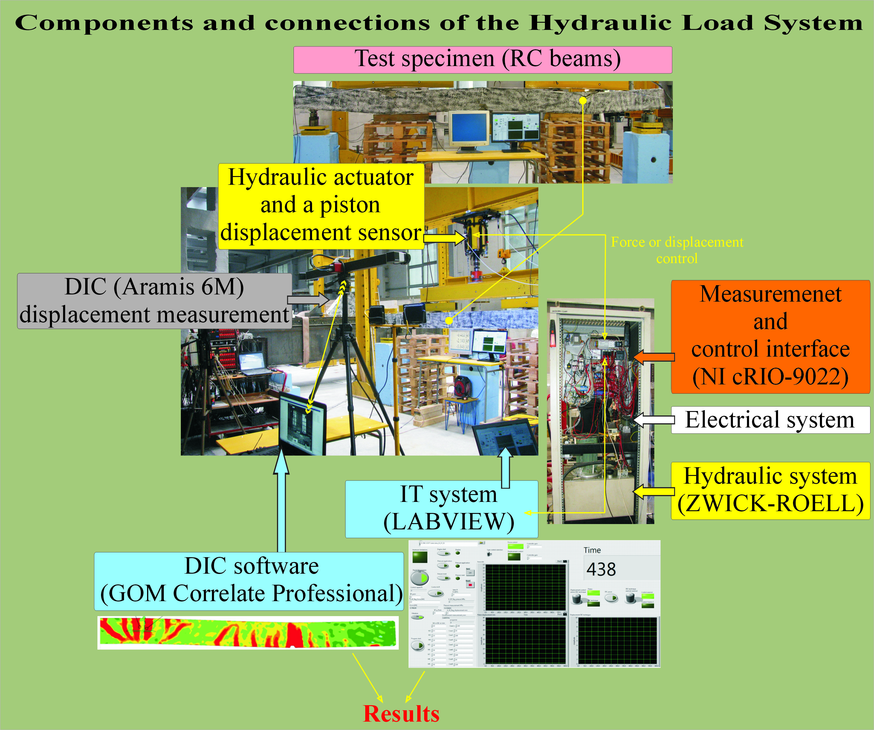
:Displacements or deformations of materials or structures are measured with linear variable differential transducers (LVDT), fibre optic sensors, laser sensors, and confocal sensor systems, while strains are measured with electro-resistant tensometers or wire strain gauges. Measurements significantly limited to a point or a small area are the obvious disadvantage of these measurements. Such disadvantages are eliminated by performing measurements with optical techniques, such as digital image correlation (DIC) or electronic speckle pattern interferometry (ESPI). Many devices applied to optical measurements only record test results and do not cooperate with the system that exerts and controls load. This paper describes the procedure for preparing a test stand involving the Digital Image Correlation system ARAMIS 6M for remote-controlled loading. The existing hydraulic power pack (ZWICK-ROELL) was adapted by installing the modern NI cRIO-9022 controller operating under its own software developed within the LABVIEW system. The application of the DIC techniques to directly control load on the real structure is the unquestionable innovation of the described solution. This led to the elimination of errors caused by the test stand susceptibility and more precise relations between load and displacements/strains which have not been possible using the previous solutions. This project is a synergistic and successful combination of civil engineering, computer science, automatic control engineering and electrical engineering that provides a new solution class. The prepared stand was tested using two two-span, statically non-determinable reinforced concrete beams loaded under different conditions (force or displacement). The method of load application was demonstrated to affect the redistribution of bending moments. The conducted tests confirmed the suitability of the applied technique for the remote controlling and recording of test results. Regardless of the load control method (with force or displacement), convergent results were obtained for the redistribution of bending moments. Force-controlled rotation of the beam section over the support was over 50% greater than rotation of the second beam controlled with an increase in the displacement.

1. Introduction
A precise determination of mechanical parameters of materials and structure behaviour is crucial from the perspective of safety and reliability of the construction process. Operations aiming at developing the assessment system for material effort and degradation, based on the localisation changes of deformations in a selected area of the structural member, constitute a relatively new trend of modern strength tests that are closely connected with the development of measuring techniques. Traditional methods for laboratory tests are usually based on contact measuring systems. Displacements or strains are determined in selected reference frames or at points, and thus do not reflect the full image of strain on the whole surface of the tested specimen. Test stands for non-contact measuring techniques based on optoelectronic systems have been successfully developed in recent years [1,2,3]. Direct connection of the digital image corellation (DIC) technique with control ensures the test quality independence of the test stand. The elimination of errors resulting from the test stand susceptibility is possible only for traditional testing machines (and requires regular verification) and has not been so far applied for structure testing. The optic technique determines displacements and strains of the whole surface of the tested specimen or element with or without a movement of rigid bodies [4,5]. They can be also used in static [6,7], dynamic [1,8,9], cyclically [10,11,12], fatigue [13,14], and landslide monitoring [15,16,17] variable tests. Introducing corrections into such tests is generally impossible, which makes the proposed solution innovative. The described system of a new class is resistant to errors caused by stiffness of the test stand and ensures a more precise correlation between the load and the structure response (displacement, strain, crack width). Post−processing provides colourful maps presenting test results, on which any operations can be performed. Non-invasive measuring techniques monitor conditions of the construction without interfering into its structure. The development of material damage under load is a local process observed in areas impaired by structural defects. Such points, however, cannot always be indicated at the stage of test planning. In practice, a specific area is determined where displacement or strain sensors are installed. The optic technique providing images of the superficial distribution of deformation using (DIC) or electronic speckle pattern interferometry (ESPI) has advantages brought by the identification of changes in the material structure. The DIC technique can be applied in both macro- and micro-scale testing, while the ESPI method is especially used in micro-scale testing [2,18]. The DIC technique uses images taken simultaneously by one (DIC-2D) or two (DIC-3D) digital cameras when spatial tests are performed on elements or structures. DIC-2D is most frequently used in standard testing machines and plays a role of video-extensometers during longitudinal and transverse measurements. The implementation of DIC-3D into testing machines is not common and rather used to monitor structure elements in their original environment [3,19] without load control. The ESPI set is intended for static measurements and requires that the load applied on the specimen is discontinued for the duration of taking a series of images, that is, for 3 seconds. However, this method offers very good resolution for deformation analysis of the order of 10−6. The DIC set offers measurements within a dynamic range of rates that depend on using two digital cameras with slightly poorer resolution for determining the deformation components of the order of 5 × 10⁻⁴. The possibility for taking real-time measurements was a decisive factor for choosing the DIC technique for preparing the remote-controlled test stand.
The available hydraulic systems of loading elements or structures are usually based on an increase in controlling force over time. The control of an increase in displacement or deformation over time u(t) is usually applied in testing machines [20,21]. A difference in load control also affects the obtained results. Devices imposing load during traditional methods are controlled with LVDT transducers, fibre optic sensors, laser sensors, confocal sensor systems, electro-resistant tensometers or wire strain gauges. The point access to a structure or a specimen clearly limits measurements. The DIC technique is a solution for minimizing defects of traditional methods to conduct measurements. Then, superficial or point measurements can be made for a test element to provide data for load control. Therefore, we tried to couple the optical ARAMIS 6M (GOM GmbH, Braunschweig, Germany) system for optical image correlations with ZWICK-ROELL (Zwick Roell Company Group, Ulm, Germany) hydraulic power pack to impose controlled load. NI cRIO-9022 (National Instruments, Austin, TX, USA) controller and dedicated software developed within LABVIEW system were used. It was challenging to modify the electro-hydraulic device into the mechatronic device composed of hydraulic, electrical, mechanical, IT, and optical subsystems. Such a synergic combination of different systems is a novelty which was applied to obtain an optimal device to realize tasks with better effects than in case of using individual subsystems [22,23,24,25]. The fundamental purpose of the test stand was to perform measurements on complicated and complex structures with the option of recording and controlling any structure size not applicable for traditional techniques. Statistically non-determinable continuous reinforced concrete beams were used as test elements. The beams were reinforced with steel of high ductility [26,27] to provide significant displacements and redistribution of internal forces in reinrorced concrete (RC) beams [28,29,30], RC plates [31,32], or beams strengthened with fiber reinforced polymer (FRP) materials [33] and rotations of sections over the support [34,35].
2. Development of the Test Stand
This test stand is a complex system of interactions between the following components:
- digital image correlation equipment—ARAMIS 6M,
- hydraulic system,
- electrical system,
- measurement and control interface,
- IT system.
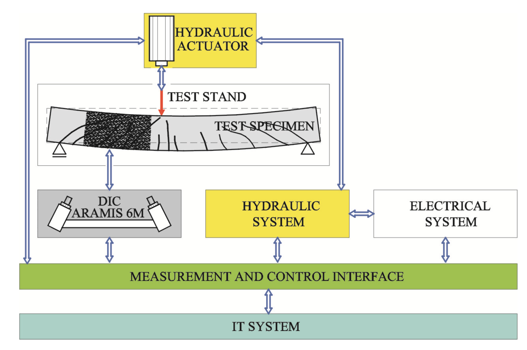
Interactions between these subsystems should be, if possible, registered and controlled. It can be generally done by using the automatic-IT system in the form of a block diagram as illustrated in Figure 1. Interactions are observed between almost all subsystems and should be taken into account to realize the set aims.
- Components of each subsystem, their mutual connections and ways of their operating are described further in the paper.
2.1. Digital Image Correlation Equipment– ARAMIS 6M
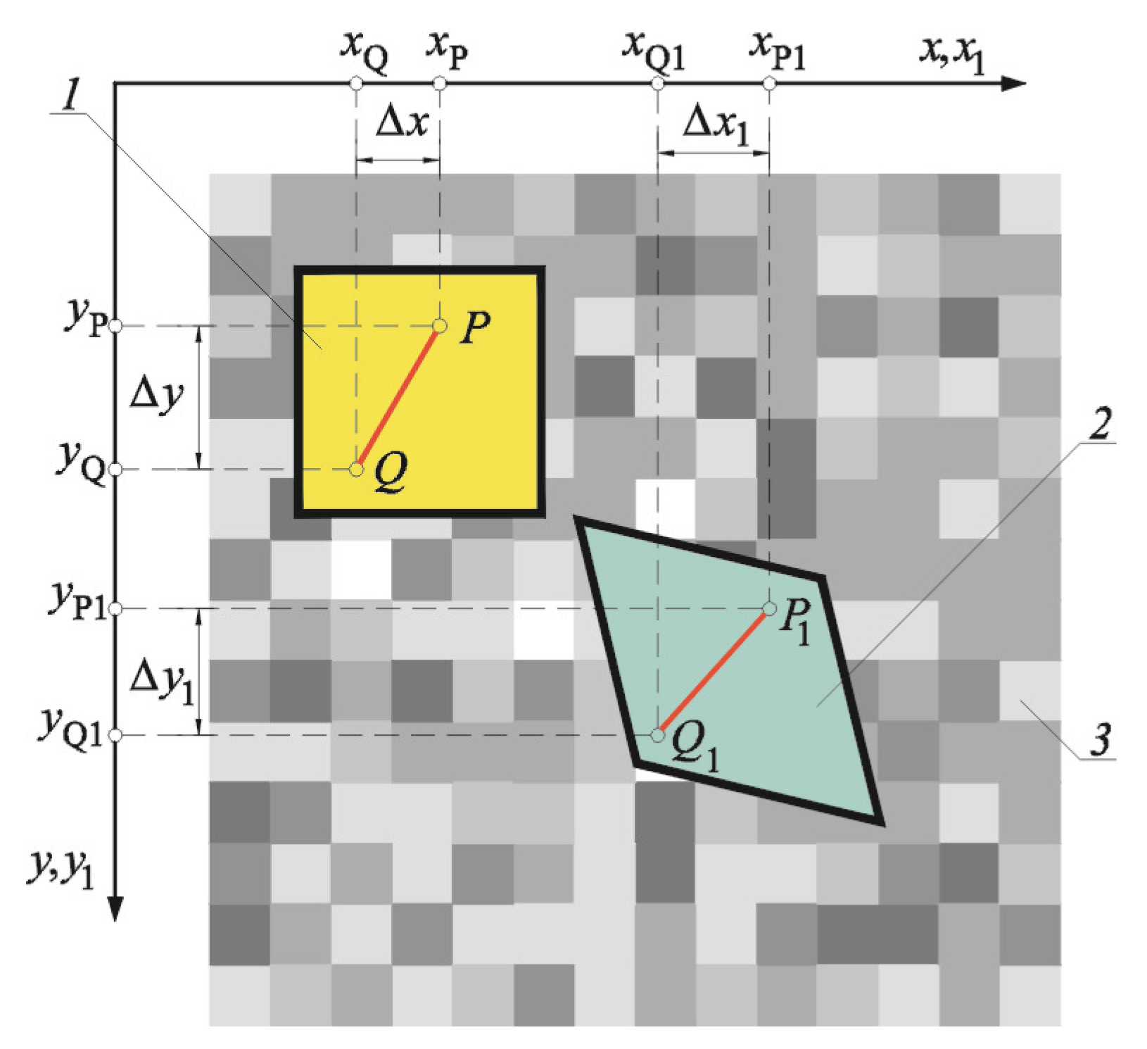
Digital image correlation devices are intended for non-contact measurements of changes in components of displacement/deformation in two- and three-dimensional systems of coordinates. When compared to other measuring techniques, such as strain gauges, the DIC technique requires the relevant preparation of measuring surface of the specimens and calibration in accordance with the applicable procedure. Digital image correlation sets include, but are not limited to, systems for analysing large (Aramis 6M) and small (Micro-DIC) deformations. Regardless of the intended use of the DIC systems, principles of their work are based on close relationships specified for the mechanics of continuous media. The principle of the DIC technique was developed from fundamentals of the mechanics of continuous media [4,36]. The analysis includes changes in dimensions and location of short segments determined by positioning two points before (P, Q) and after (P1, Q1)—deformations, as shown in Figure 2. Components of the deformation tensor could be determined if changes in the length of sections are known. The undeformed surface, shown in Figure 2, in the DIC procedure is analysed by assigning coordinates to individual small areas (pixels). Separating the undeformed reference zone is the next step. Changes in shape and location of that zone are analysed while load is applied and recorded in the system of 0xy and 0 × 1y1 coordinates.
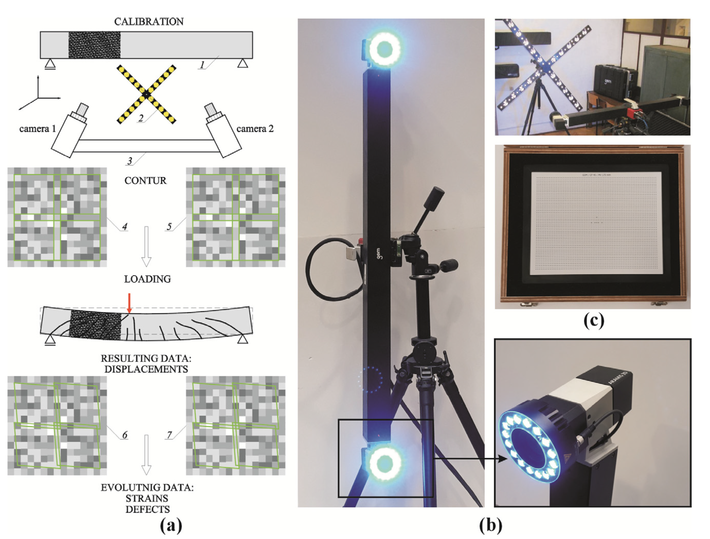
The ARAMIS 6M system used at the test stand was equipped with two digital cameras (Figure 3), each with the resolution of 6MPx. One camera provided two-dimensional results. Time required for obtaining the end result was much shorter than in the configuration of two cameras. The measuring area suitable for the analysis with the Aramis 6M system should range from 150 × 170 mm to 2400 × 2400 mm. Each test was preceded by calibrating the device with a calibration plate or cross (Figure 3c) containing typical reference points and points of an object in the unloaded state. Coordinates of points in the central part of the calibration plate or cross had to be given greater values of coordinates than values of other points to ensure the calibration validity.
The whole process was based on the correlation principle and the method of searching points of the same coordinates. At first, the contour was defined for the analysis and its shape, for which characteristic points of the analysed layer were assigned to square or rectangular areas of 15 × 15 pixels (known as “facets”), was recorded. The separated segment of a measuring area included facets of 15 × 15 pixels, as well as the so-called common areas with the width of 2 pixels towards each direction. Common areas were used to reduce an error in measuring strains as each analysed area (facet) contained elements from the adjacent area and the same boundary conditions. The determined values of displacement components for individual points were used to calculate components of strain/stress in the form of the field image. The DIC system was used to determine coordinates of the 2D system on the basis of reorientation of the midpoint of the facet rectangle/rhombus. Coordinates determined with both cameras and an angle between their axes can be used to describe coordinates of the 3D system [37]. The ARAMIS 6M system used for image analyses involved the model based on the normalized cross-correlation (NCC) ρ [38,39,40]. The NCC ρ was calculated between the initial and current location of each pixel. The value ρ was calculated as a discrete function of changes in displacements (Δx, Δy) and average values from grey areas and compared pixels. The closest location was chosen (at the pixel level) by choosing the minimum value of the common NCC. The function of NCC was estimated within the searched area, and its maximum indicated the best match. It should be also mentioned that the DIC technique also uses the method of least squares, which also included rotations of points [5,41]. The best match is defined by minimising a difference in grey intensity between two consecutive analysis windows using the method of least squares.
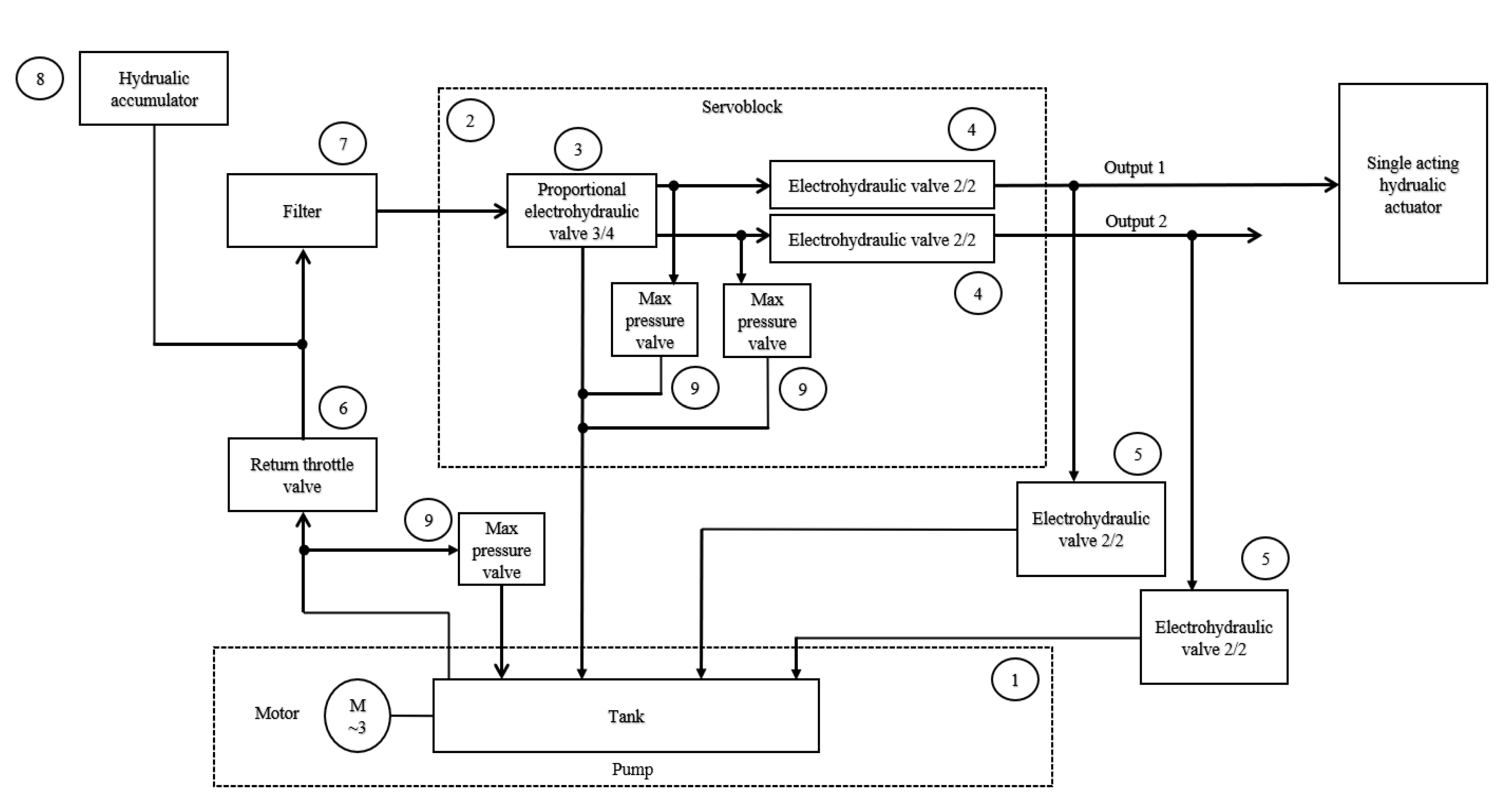
2.2. Hydraulic System
The hydraulic subsystem consisted of a hydraulic pump with constant efficiency (No. 1 in Figure 4) by ZWICK-ROELL, driven by 3-phase asynchronous motor with 3 kW power. The main component of the hydraulic subsystem was a hydraulic servoblock (No. 2) consisting of:
- A proportional electrohydraulic valve (No. 3) to control flow in a hydraulic circuit. The modified control and the measurement system were used to control the flow of working medium in the hydraulic system by adjusting the proportional electrohydraulic valve with PWM signal. The system was controlled with CompactRio controller by National Instruments company. That solution ensured the indirect steady control of pressure at outputs supplying driver elements.
- Two bistable two-way electrohydraulic valves with a return spring (No. 4). Both elements were operating in either open or close position. Working medium in the open position was delivered to the output (supplied the driver element) in contrast to the close position, in which the medium was not delivered to the output. These valves were controlled with 0–24V digital signal.
- Another two bistable two-way hydraulic valves (No. 5) were between the hydraulic servoblock and the driver element (hydraulic actuator). They were used as drain (check) valves for hydraulic working medium delivered from the supply system of driver elements. The valve switching between two positions (open and close) was analogous to the above described process (with digital signal).
That configuration was suitable for controlling two single-acting hydraulic actuators (individually connected to two outputs, marked in Figure 4 as: Output 1 and Output 2) or one double-acting hydraulic actuator (connected to both outputs). Additional elements of the hydraulic systems were:
- A manually controlled return throttle valve (No. 6) used as pressure regulator at the pump output and protecting the system against a change in flow direction of working medium.
- A filter (No. 7) used as the cleaning system for various types of contamination.
- The system of two hydraulic accumulators (No. 8) was the additional source of energy for the hydraulic system at an increased demand on energy, and also eliminated pressure pulsation of working medium.
- Three hydraulic safety valves (No. 9) to provide protection against too high pressure in the hydraulic system.
- The block diagram of the hydraulic system is illustrated in Figure 4.
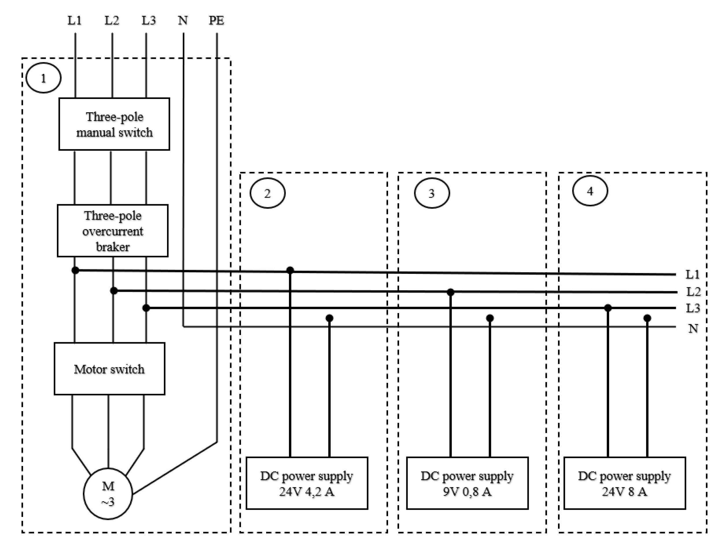
2.3. Electrical System
The electrical system consisted of four circuits; one three-phase alternating current circuit and three independent direct current circuits of 24 V (two circuits) and 9 V (one circuit). The block scheme of the electrical system with individual circuits is illustrated in Figure 5. The AC circuit (No. 1 in Figure 5) contained the main three-pole manual switch, the three-pole overcurrent breaker and the electromagnetic contactor controlled by 24 V direct current with additional overcurrent protection.
Two independent DC circuits of 24 V nominal voltage (No. 2 and 3 in Figure 5) were used to separate the power supply system for the IT subsystem from electric driver elements (electrohydraulic valve coils, motor-rate contactor coil). That operation increased reliability of the whole system. The third DC circuit (No. 4) of 9 V nominal voltage supplied the modulus of PWM generator, producing the signal for controlling the proportional electrohydraulic valve.
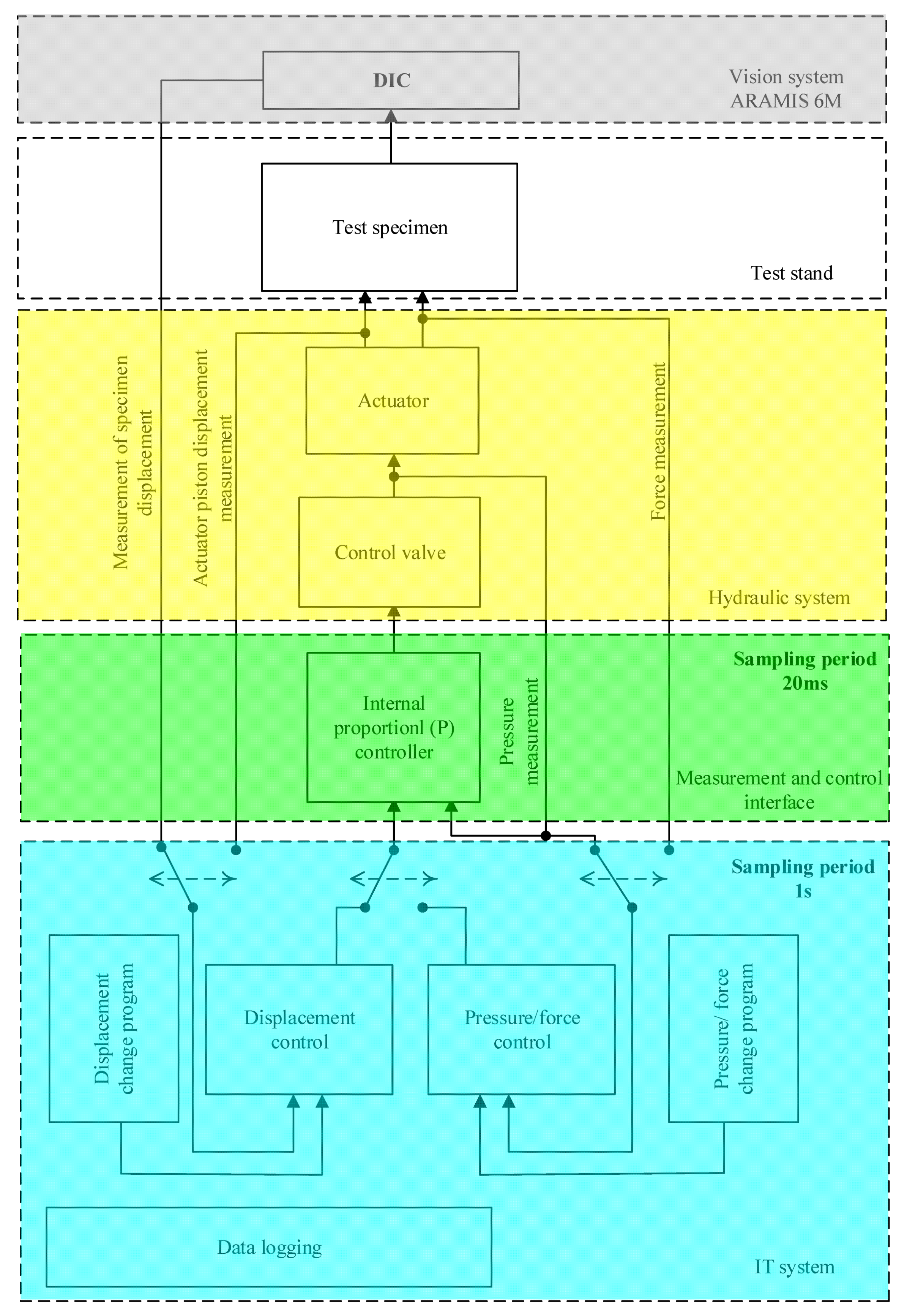
2.4. IT System and Measurement and Control Interface
Interactions with the measurement and control interface were crucial for the IT system which only communicated with the interface. Regarding the equipment aspect, the measurement and control interface involved the CompactRio controller (by National Instruments) and the measuring modules. The IT system was run on PC with LabView software (by National Instruments). LabView is the advanced programming language used to implement different types of control algorithms [42] and is applied not only at an experimental stage, but also in professional testing devices. LabView and the CompactRio controller make an effective testing tool for laboratory stands [43].
In accordance with intention of the authors, the system had to perform functions for ensuring safety and performing experiments. The safety functions were carried out by the measurement and control interface by providing the complete lock of the system in case of situations identified as dangerous. Pushing a safety button or end position of the actuator piston can be classified as such situations. The functions for performing experiments had to ensure that the schedule was met as precisely as possible. Therefore, they were also performed by the measurement and control interface operating with short sampling time of 20 ms. The deterministic operation of the whole system with the short sampling time could effectively fulfil functions for safety, low-level control, as well as lossless filtering. The IT system was operating within the sampling period of 1 s and had the user-friendly interface, superordinate control loop and data storage. Taking into account the performed tests, shorter sampling time for the IT system was not necessary. And the measurement and control interface, which should operate quickly, was not overloaded by communicating with the IT system. The schematic diagram of the system operation is illustrated in Figure 6.
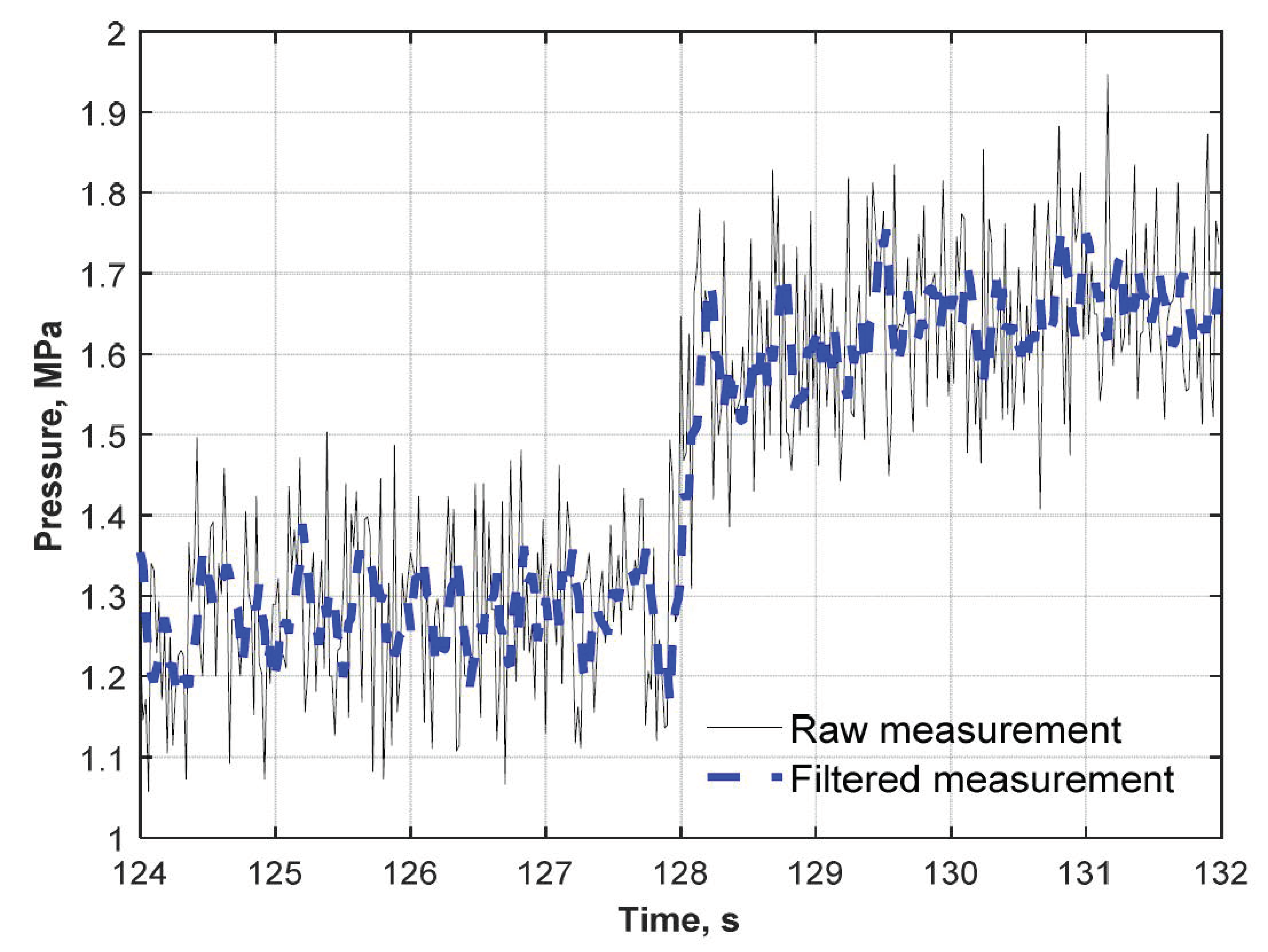
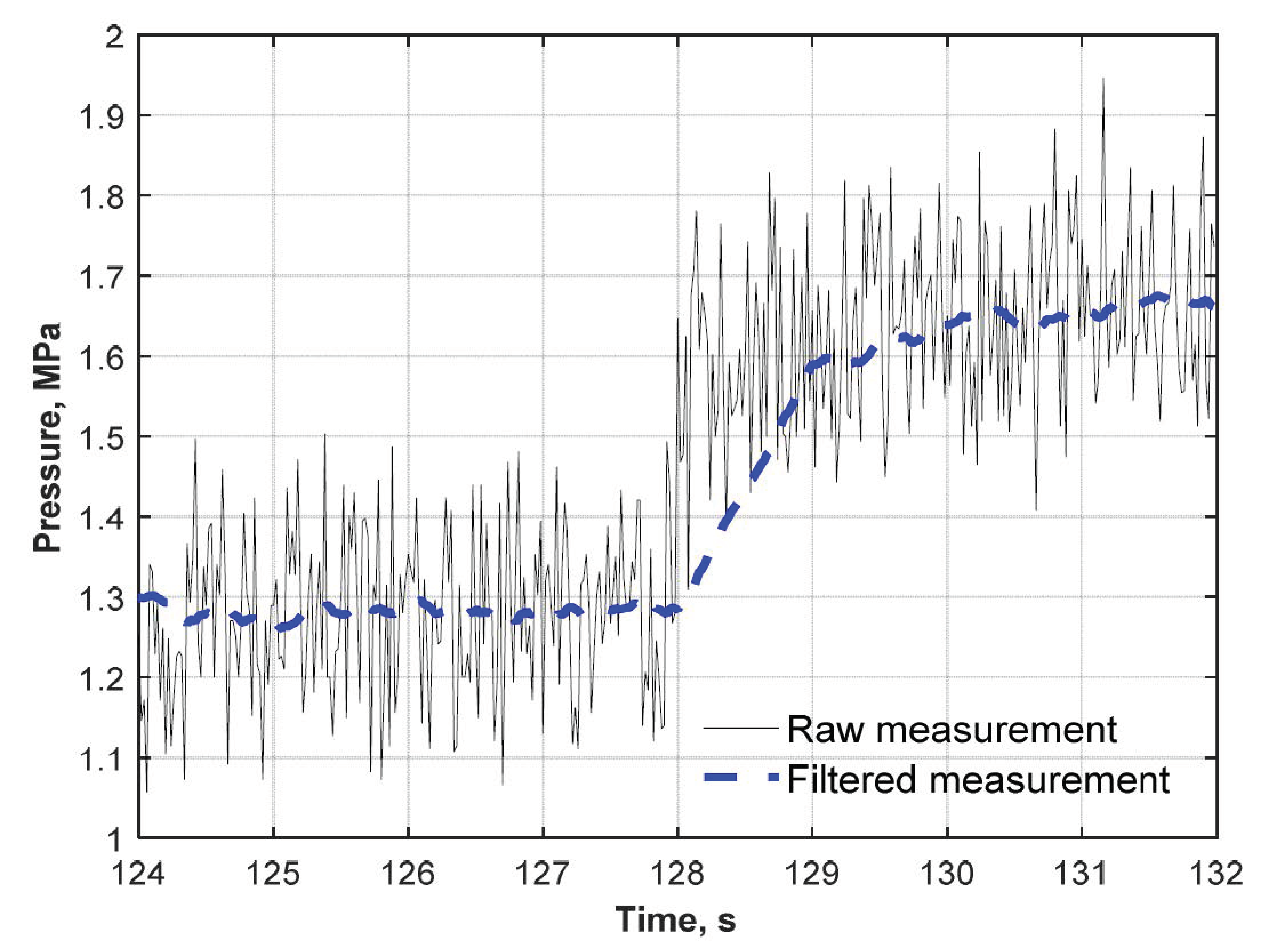
In respect of the quality control, measuring accuracy and the analysis of individual signals [44,45], particularly in the bottom range of the system, are significant. These aspects were crucial during tests performed on the specimens, for which relatively small acceptable loads were expected. Hence, correct filtering of signals was important which was discussed in the papers [46,47]. Regardless of the chosen methodology, the adequate range of approximation was significant and determined filtering potential [48]. The multi-piston pump at the test stand generated pulsatory pressure around a certain mean value. Additionally, measuring noises interfered with the variable signal. A sum of these events caused that recorded changes in pressure maintained at the constant level did not exceed 0.45 N/mm2 (Figure 7).
When a moving average for the range of approximation for five specimens was used, the oscillation in signals was significantly reduced at maintained acceptable dynamics of an operating point. It is shown with a blue broken line. The pressure signal was used internally at the level of the measurement and control interface to stabilize pressure at the control valve with a short sampling period, for which the signal dynamics was very important. In that case further filtering could not be continued due to the correct operation of the system. But the signal sent to the IT system required further filtering to obtain practically “smooth” average value. For that purpose, a filter was used with a greater range of approximation of, in that case, 50 specimens (Figure 8), which still did not generate loss as far as the IT system reading data every 1 s was concerned.
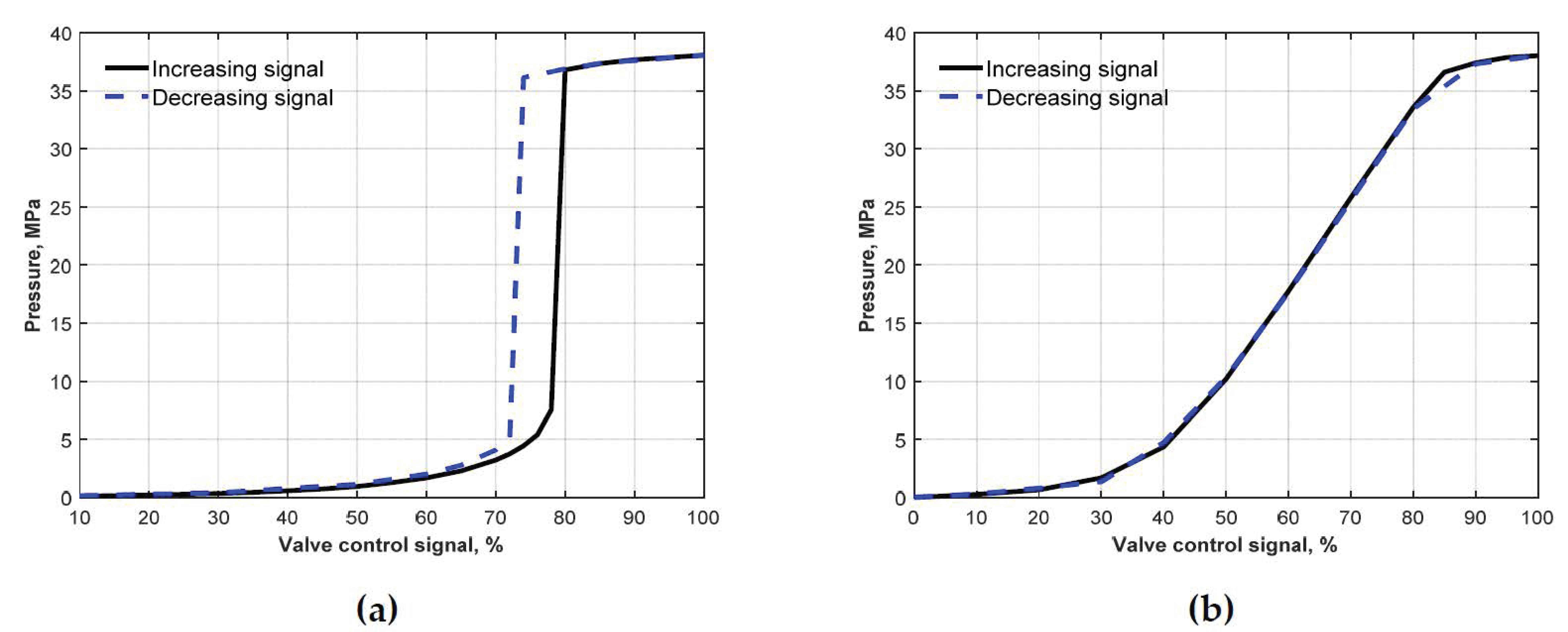
In that case the cascade control was recommended [49,50]. The cascade control structure has been known for many years [51]; however, it is still developed [52,53] with reference to the control structure and tuning methods. The control structure can be adjusted to a given object, and delays can be properly taken into account. The recent papers [54] have focused on tuning that provides very high control quality at the expected sensitivity. In some cases, it is reasonable to add an adaptive model-base regulator into the cascade control structure to deliver further improvement in the control. Although these control structures are advanced, they are implemented using the standard PLC platforms [55,56]. Hence, the valve was also under the linearized negative feedback. That function was performed by the internal regulator P (shown in Figure 6). Consequently, different characteristics presented in Figure 9b were obtained with significantly smaller non-linearity without the hysteresis zone.
Measurement errors and their characteristics were estimated by measuring pressure without an operating pump. The quality of pressure measurement was tested at constant zero pressure with the sampling period of 20 ms. The obtained average value was 0.0408 MPa and the standard deviation was 0.1110 MPa. The standard deviation was tested at different non-zero values of pressure and the obtained values were within the range of 0.1110–0.1116 MPa. Therefore, the standard deviation was assumed to be constant regardless of the measured pressure. In case of the filtered signal, the standard deviation was significantly reduced to 0.0488 MPa using the proposed filter with the width of five specimens. A double broadening of the filter window reduced the deviation to 0.034 MPa which was a small improvement with reference to deteriorated dynamics of signal tracking. Therefore, the selection of the filter with the width of five specimens was proved to be correct.
As the DIC system software was connected with the measurement and control system through the analog signal of 0–10 V, it was necessary to verify the standard deviation of the transmitted signal. Standard results for measuring displacements without filtering for a few test specimens were within the range of 0.0125–0.0155 mm. That result gave satisfactory accuracy of stabilizing displacement measurements.
Besides the measurement accuracy, another aspect regarding the control quality was the characteristics of the hydraulic system used to apply load. The system consisted of the pump, the control valve, and the actuator. Some parameters of the pump and the actuator (not directly stated in data sheets provided by the manufacturers) were empirically determined: volumetric flow of the pump V* = 3.46 [l/min], pressure fluctuations resulting from the pump operation were ca. 0.41 MPa. It should be emphasized that the obtained pressure 0.41 MPa was an instantaneous value contributing to only 1% of the pump operating range (the maximum range was 400 bar (40 MPa), defining the worst possible case. Pressure was measured directly at the pump output at the cut-off actuator. Measured pressure fluctuations were significantly suppressed by combining hoses with the actuator. Hence, high pulsation of the force acting on the test element (the obtained value was confirmed by measuring forces with the electro-resistant dynamometer) was not observed. The static characteristic of the control valve in the open loop, which is illustrated in Figure 9a was experimentally verified. Very high variability of the valve amplification and the ambiguity of the data sheet in the form of the hysteresis zone were troublesome.
The above procedures provided the control system adequately prepared for the operation. Regarding the control theory, this system had a cascade structure with different sampling times at the level of internal and external control loop. The direct control of the pressure or the displacement was possible, but its precision was not so precise due to delays and non-linearity. The stabilisation of pressure at the pump output was necessary to achieve the required control precision. Pressure measurement was quick and accessible. Therefore, the internal control loop could be carried out to stabilise pressure. Measurements were taken at high rates (every 20 ms) which enabled a quick response to pressure changes by a proportional controller which did not introduce the extra dynamics, but caused linearization of pressure from the pump. A large number of measurements (50 within a minute) was sufficient to average 50 measurements, which provided a satisfactory filtration, generally lossless when considering the IT system used to sample the internal system (measure and control interface) every second. Based on the testing programme and the current measurement e.g., displacement of the test element, the master control system sent the set value of the internal controller stabilising pressure. Due to such a structure, the control was much more precise as the slower signal path (changes in displacements) did not have to react to quick pressure interference. Additionally, the object behaviour was nearly linear despite high non-linearity of the pump (Figure 9a,b). The concept of the cascade control is well known. But the method of its application to conduct a relatively slow measurement with the DIC technique to effectively control the displacement is a novelty. From the mechanical point of view, an important originality of the developed control system lay in eliminating the impact of the test stand susceptibility on test results. Generally, changes in the loading force resulted in recording piston displacement that was regarded in testing machines as strain in the test sample (construction) and the structure displacement measured with the DIC technique. The measured displacement of the structure used as the reference effectively eliminated an error caused by the test stand susceptibility.
3. Test Stand Validation
3.1. Test Models
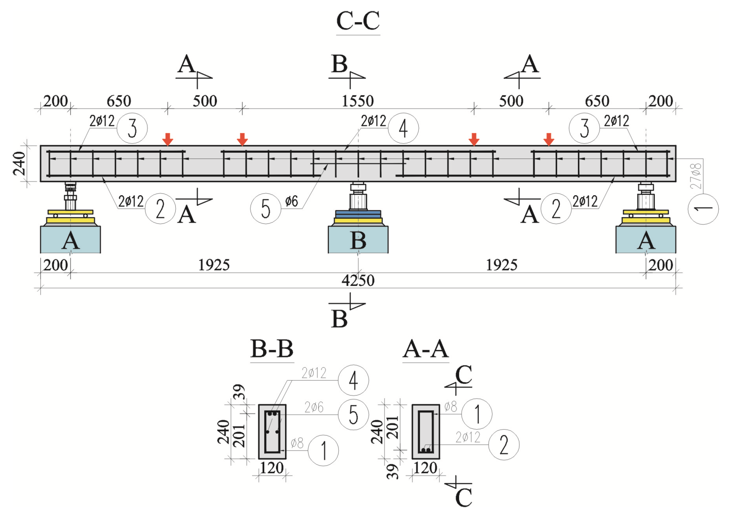
To highlight possibilities of the prepared test stand, two statistically non-determinable beams with constant geometry, identical concrete strength and reinforcement structure loaded in the same mode were used as test elements. The beams were marked as “Beam No. 1” and “Beam No. 2”. The beams (Figure 10) had cross-section dimensions of 0.12 × 0.24 m and the total length of 4.25 m.
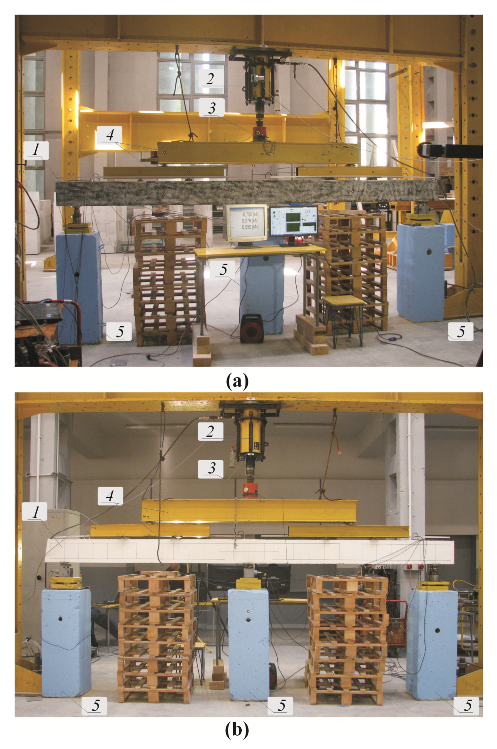
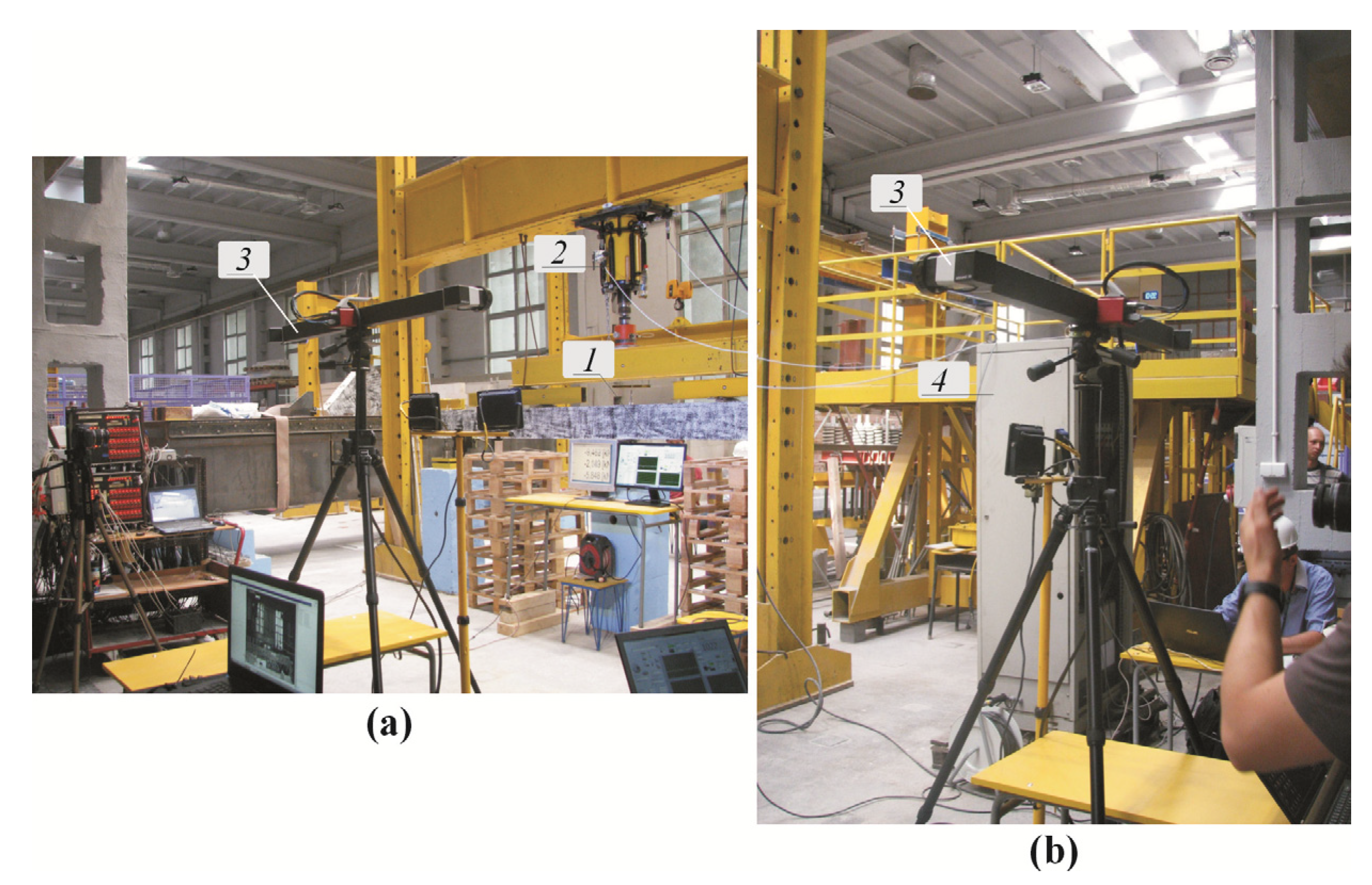
The beams were supported symmetrically every 1.925 m. The models were reinforced with longitudinal bars φ12 mm and stirrups φ8 mm. Adhesion anchorages were used for longitudinal bottom (2) and top (3) beams under tension. The same span reinforcement 2φ12 mm (ρ1 = 0,174%) and the reinforcement above the support was applied in all beams. Transverse reinforcement (made from the same steel type and longitudinal reinforcement) consisted of stirrups (1) perpendicular to the beam axis φ8 mm. The position of stirrups in the over-support section (80 cm in length) was stabilized with wires φ 5 mm made of St0S steel and placed in the centre of beam cross-section (12 cm from horizontal edges of cross-section). The cover size of all rebars in the longitudinal reinforcement was cnom = 25 mm, and in the transverse reinforcement cnom = 15 mm. The reinforcement was made of B500SP steel rebars (Epstal). Symmetrical load with four concentrated forces was assumed to be exerted on each span of the beams. The orientation of concentrated forces was chosen to represent as closely as possible the uniformly distributed load imposed by two concentrated forces. All beam surfaces were painted with white emulsion that eliminated pores and surface irregularities. Then, black spots were randomly applied on one surface to perform optical measurements with the ARAMIS software. A plastic brush with hard bristles was used to apply these spots, as shown in Figure 11a. Another side of the beam was used to represent the reinforcement—Figure 11b and take inventory of crack morphology. A view of elements of the test stand is shown in Figure 12.
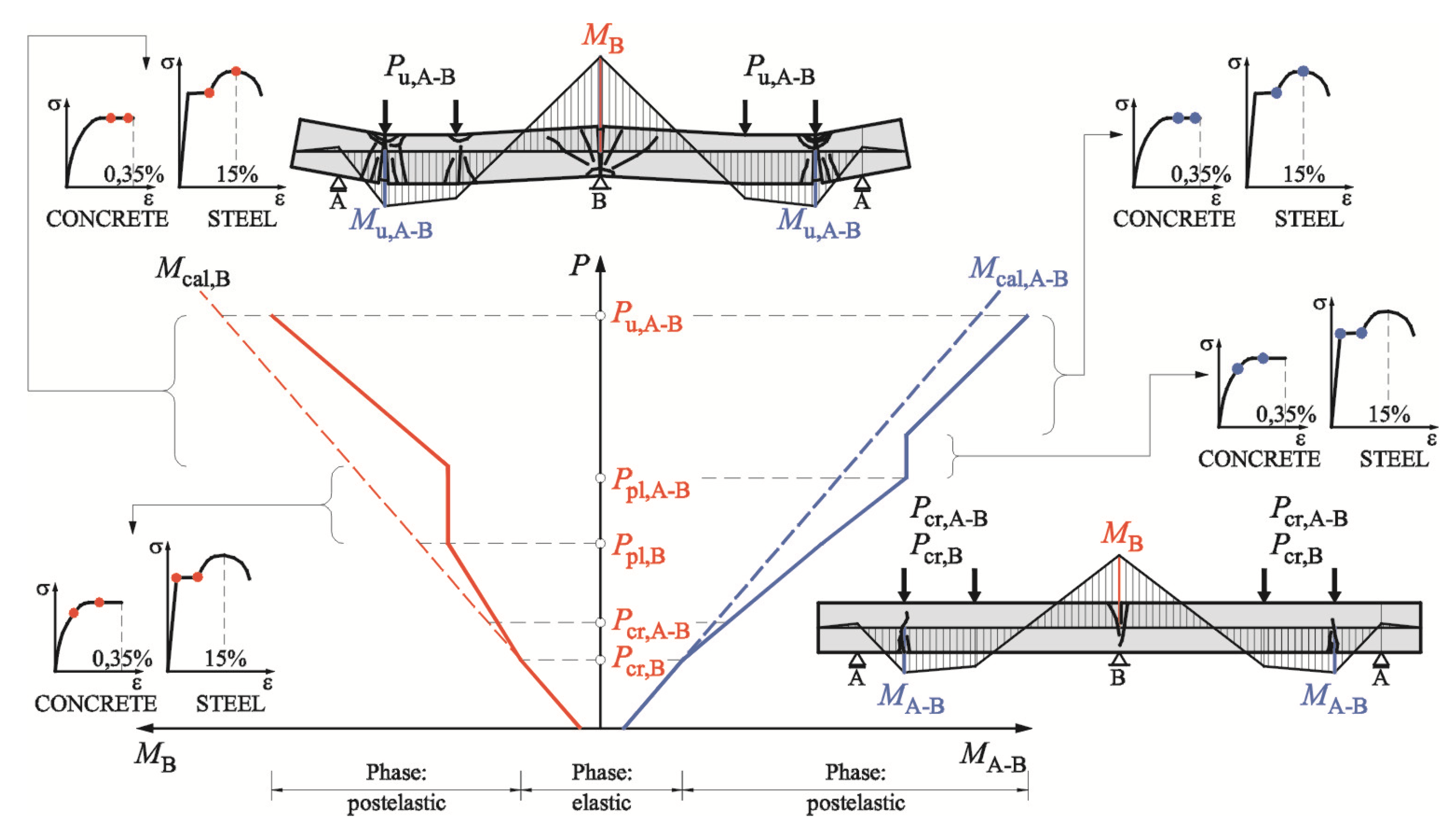
The statically non-determinable beams under different load conditions were used to demonstrate changes in the redistribution of a bending moment at relevant sections. Figure 13 presents the probable course of bending moments in the span and over the support. Bending moments in the elastic phase until cracking corresponded with the calculated values. An increase in span moments could be expected in the period from cracking over-support and span sections until plastification of the support reinforcement when support moments are determined and slightly reduced. Values of bending moment over the support were expected to be constant at the time of reinforcement flow. A further increase in loading would result in an increase in bending moments in the spans, i.e., a redistribution of bending moments. At the time preceding the failure, large cracks over the support and in the span were assumed. The beams were loaded monotonically until the failure using the load procedure adjusted to potential of the developed load system. The concentrated force P from the hydraulic actuator was distributed by four identical forces, two per each span. The cracks were continuously monitored throughout the tests and values of the force inducing cracks visible to the naked eye (w > 0.05 mm) were read for the area over the support Pcr,B and in the span Pcr,A-B. Destructive force Pu value was read at the time of failure. The control with the ARAMIS system only referred to one span of each beam due to the length of beams (the applied measuring area was 2400 × 2400 mm). Although the system was equipped with two cameras and 3D measurements could be taken, only measurements in a beam plane, DIC-2D, were conducted in the tests. The ARAMIS software was used to observe the morphology of cracking, record displacements, and rotations.
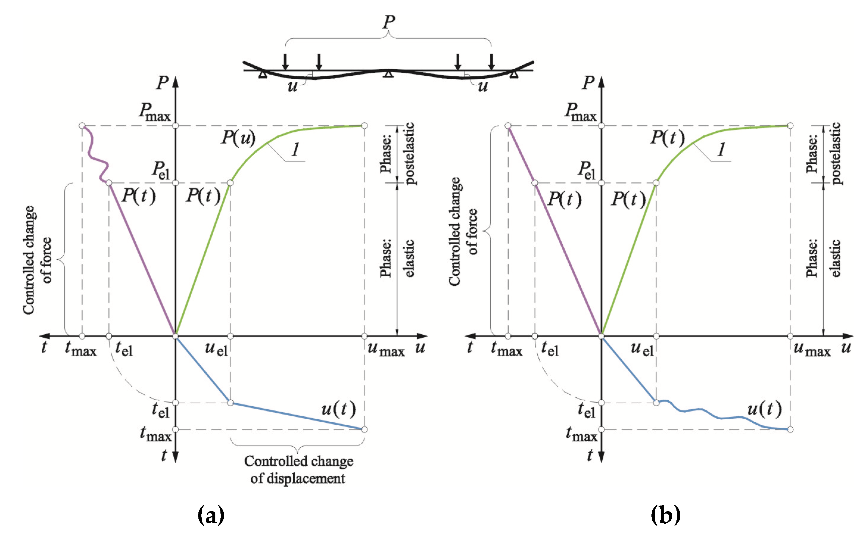
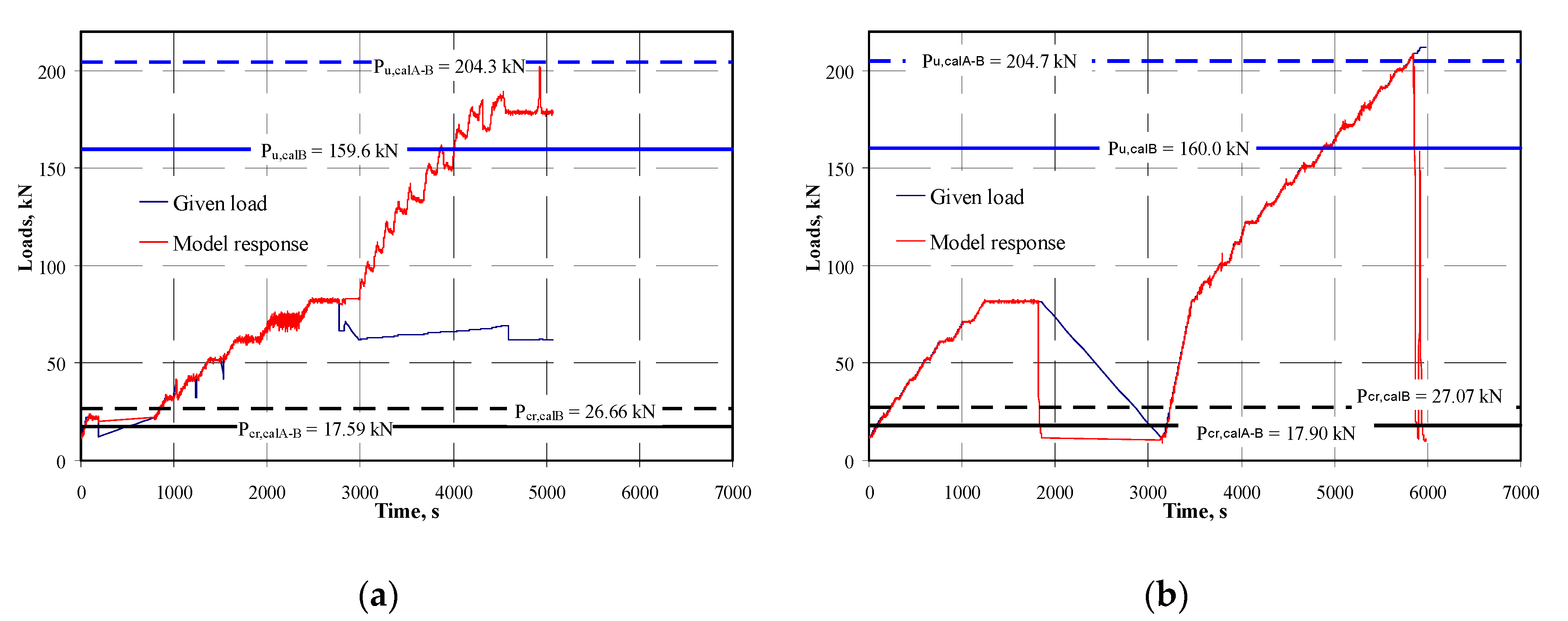
Different methods of the load control were used in both beams. In the initial phase, in which the beams behaved in the linear-elastic manner, the load was applied at a controlled increase in force over time P(t). In the subsequent phase, an increase in the displacement of Beam No. 1 over time u(t) was controlled, whereas in case of Beam No. 2 only an increase in force over time P(t) was controlled. Different methods of controlling the load were expected to produce a clear redistribution of bending moments in Beam No. 1 in contrast to Beam No. 2. The testing programme for both beams is shown in Figure 14.
3.2. Software Settings
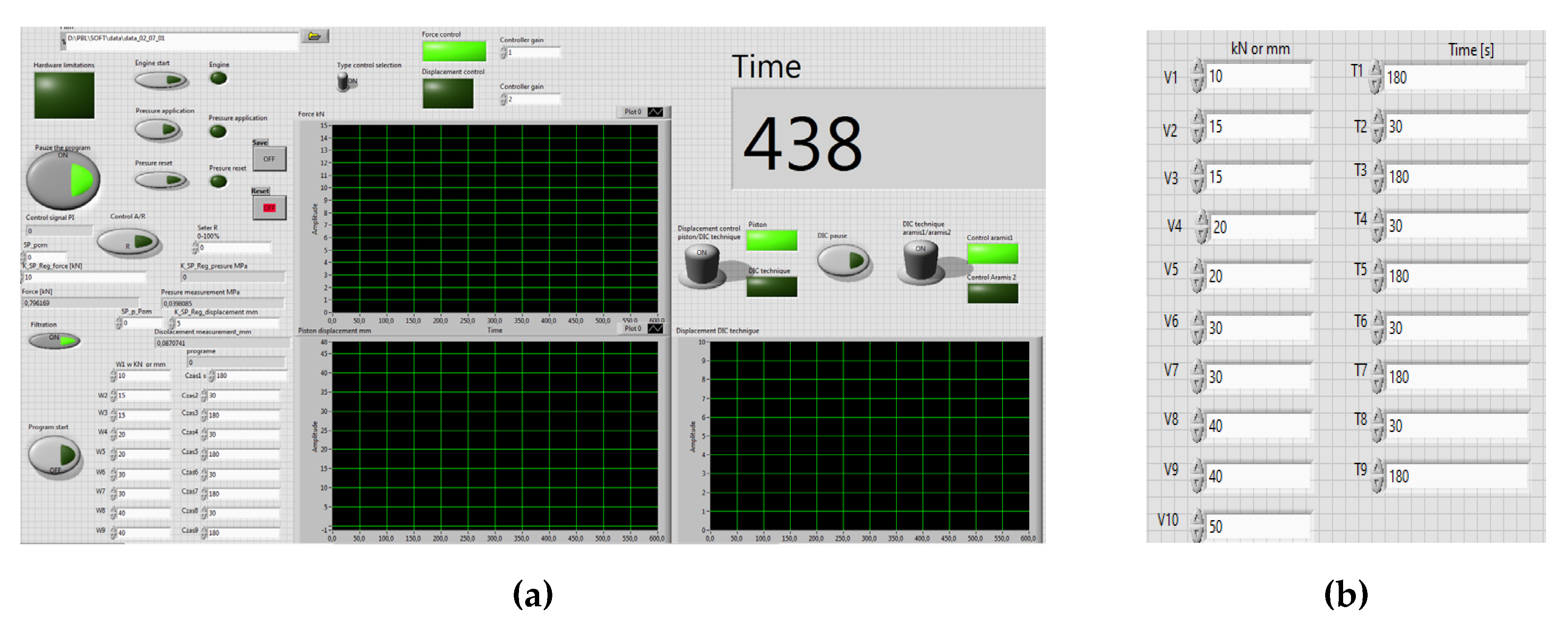
The developed software recommended for the stand was designed to perform tests on its individual elements, and to configure and conduct tests in accordance with the schedule. The first stage included the activation of the test stand and the verification of its safety, which were obligatory before conducting any tests. Then, it was required to specify measurements included in the control procedure. As shown in Figure 6, displacement could be controlled with the optical measurement using the Aramis software or on the basis of displacement of the actuator piston. These three graphs can be used to track the force, piston displacement and measurements taken with the DIC technique. The software offers a range of selection functions of control type in accordance with the logic shown in Figure 15a. As in case of controlling, the force imposed on the test specimen could be measured in a direct mode or indirectly on the basis of pressure applied to the actuator. Default parameters of filtering measuring signals could be changed. The development of the software with the intuitive interface was the most important part of the preparation works for the tests. The testing programme was used for entering pairs of V and T values. V value meant the expected displacement or force, and T value was time, during which the value was to be changed linearly with reference to the next V value. In accordance with the example presented in Figure 15b, the baseline was V1 = 10k N and was expected to change linearly over time T1 = 180 s to the value V2 = 15 kN. Values V2 and V3 were the same, which means that force of 15 kN was kept for T2 = 30 s. Then, the force value was increased to V4 = 20 kN over time T3 = 180 s. In case of a drop in these values, the next V value should be smaller than the preceding one.
When the programme was set, it could be activated. From that time the system autonomously realized the control programme. The programme could be stopped at any time due to safety reasons or on the request of an operator. In case of its interrupting, the procedure of activating the programme had to be conducted from the beginning. The operator also could stop the programme which was put into the “frozen” state, and the pressure force or element displacement was kept at the level, at which the programme was interrupted. The programme could be restarted and continued at any time.
3.3. Identifying Measurement Errors and Determining Values of Correction Factor
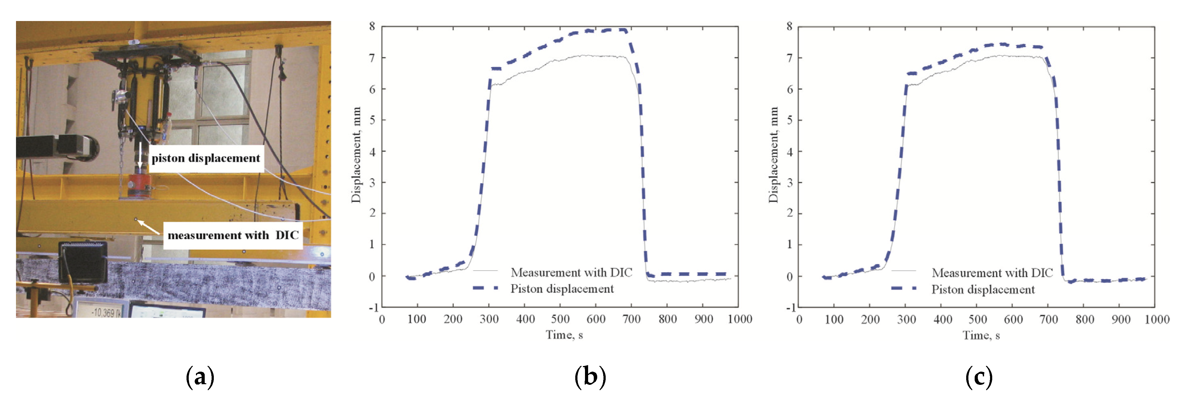
Prior to the main tests, displacements of pistons in the hydraulic actuators and steel cross beams were measured using the DIC technique (Figure 16a). Figure 16b illustrates a difference in results from measuring piston extension with traditional LVDT transducers (reading range ±10 mm and accuracy ±0.001 mm) and the DIC technique. A difference in indications exceeded 1 mm in extreme situations, which was a significant measurement error (>12%).
If the DIC technique cannot be used for a given experiment and the characteristics of deflection of the top bottom beam from the test stand is known, then the additive correction factor can be introduced to the IT system to make measurements with the LVDT transducer. Thus, the obtained measurement was more precise, but not so precise as in case of using the DIC technique.
The correction factor obtained in the above way was summed with results from measuring displacements of the piston extension. Examples of the obtained results of displacements in the actuator piston and the correction factor are presented in Figure 16c. In spite of introducing the correction, the error of indications was reduced by more than 50%. However, the absolute difference in displacements was significant using the traditional measuring technique as it exceeded 0.5 mm, and the maximum error was 6%, which was considered as acceptable in structure testing.
To sum it up, the use of the correction factor was very much advised for the results obtained from the traditional measurements. However, as the tests showed, the factor did not eliminate differences in measuring displacements of the structure itself using the DIC technique. The employed DIC technique is the precise method of measuring the structure displacements and is not affected by external factors related to the observed susceptibility of the test stand, the construction clearance, and possible accidental errors. The structure was loaded by changing the extension of the piston in the hydraulic actuator fixed to steel frames of the test stand. Consequently, the structure displacements were observed and measured with the DIC technique. It was demonstrated that the errors caused by measuring the structure displacements with the LVDT transducer could not be practically eliminated due to the method error.
4. Test Results
The specimens of concrete blocks having dimensions of 150 × 150 × 150 mm were tested on the day of testing each beam. Other concrete parameters were calculated in accordance with the standard EN 1992–1–1:2010 [57]. The average concrete strength in Beam No. 1 was fcm = 57.6 N/mm2, and fcm = 59.3 N/mm2 in Beam No. 2. The corresponding compressive strength of concrete was fck = 49.6 N/mm2 and 51.3 N/mm2 respectively. Also, raw rebars were tested to determine their yield point and tensile strength. The obtained values for longitudinal rebars of 12 mm in diameter were Re = 629 N/mm2 and Rm = 770 N/mm2. For the stirrups, they were Re = 629 N/mm2 and Rm = 732 N/mm2. Deformations at the greatest force were Agt = 15.5% (φ12) and 16.1% (φ12). The tested steel was classified to class C in accordance with the Eurocode [57].
Table 1 presents test results for the beams in the form of cracking and failure forces and corresponding values of bending moments over the support and in the span, which were calculated with respect to self-weight and equipment weight.
Figure 17 illustrates the test results for both beams as a change in the applied load and the response of the structure over time. The load applied and read from the dynamometer sensor was almost the same for both beams within the linear range of the structural movement. A clear drop in the force being the response of the structure was observed in Beam No. 1, whose displacement was controlled in the post-elastic phase. In Beam No. 2 with the controlled force increase over time, there was a slight difference between the imposed and read load values.
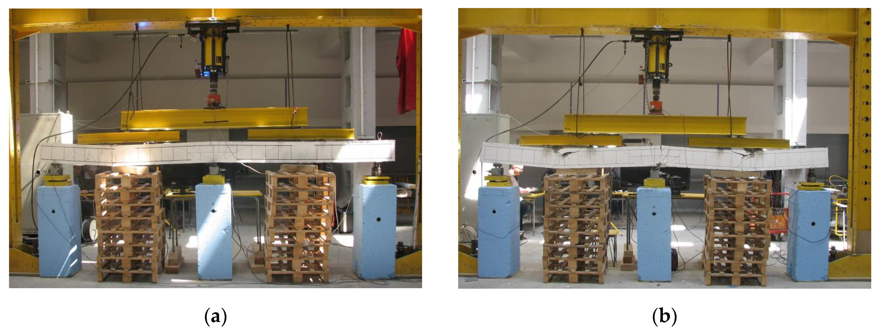
First cracks were observed at the over-support section under the total load applied to the beams equal to 20 kN. An increase in load resulted in the development of cracks over the support and new cracks in the spans closest to end supports A where the concentrated forces were imposed. Failure was rather gentle and preceded by an increase in the crack width at the support and span sections. And at the span sections at the time of failure concrete was crashed in compressed areas. The beams after tests are presented in Figure 18.
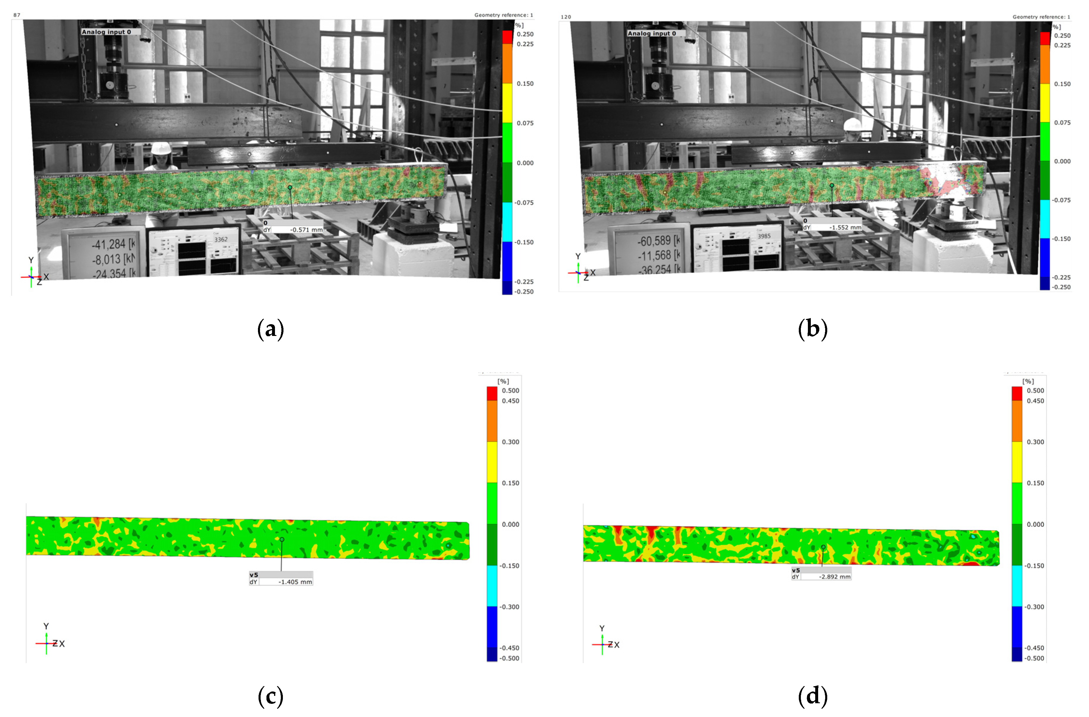
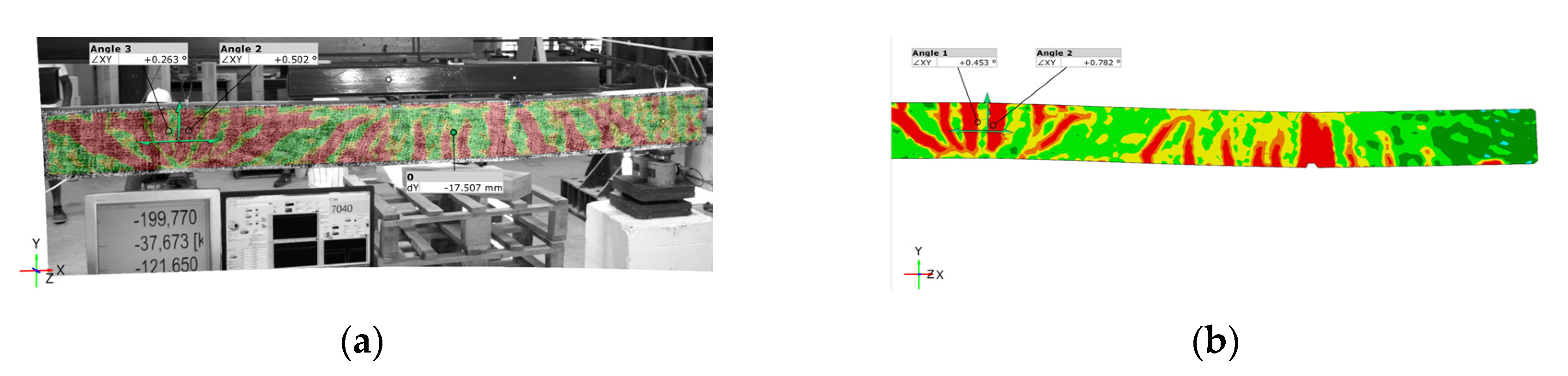
Values of deformations of the beams at the time of cracking of the support and span sections are compared in Figure 19. Rotations of the section at the support zone at a distance 0.6 × h = 144 under the greatest recorded loads is presented in Figure 20. The above scheme of loading was applied to compare the observed changes in responses from the supports and redistributions of bending moments, particularly in the phase after the formation of plastic hinges over the support.
5. Discussion
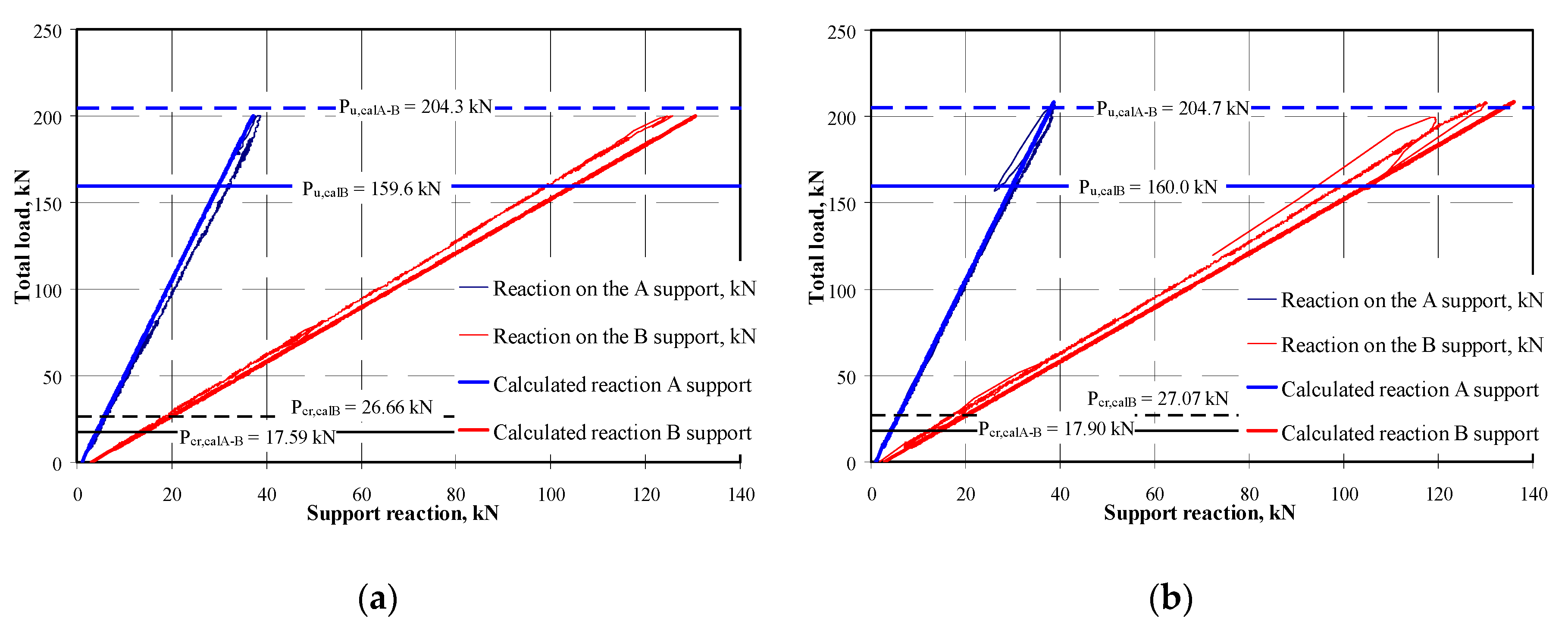
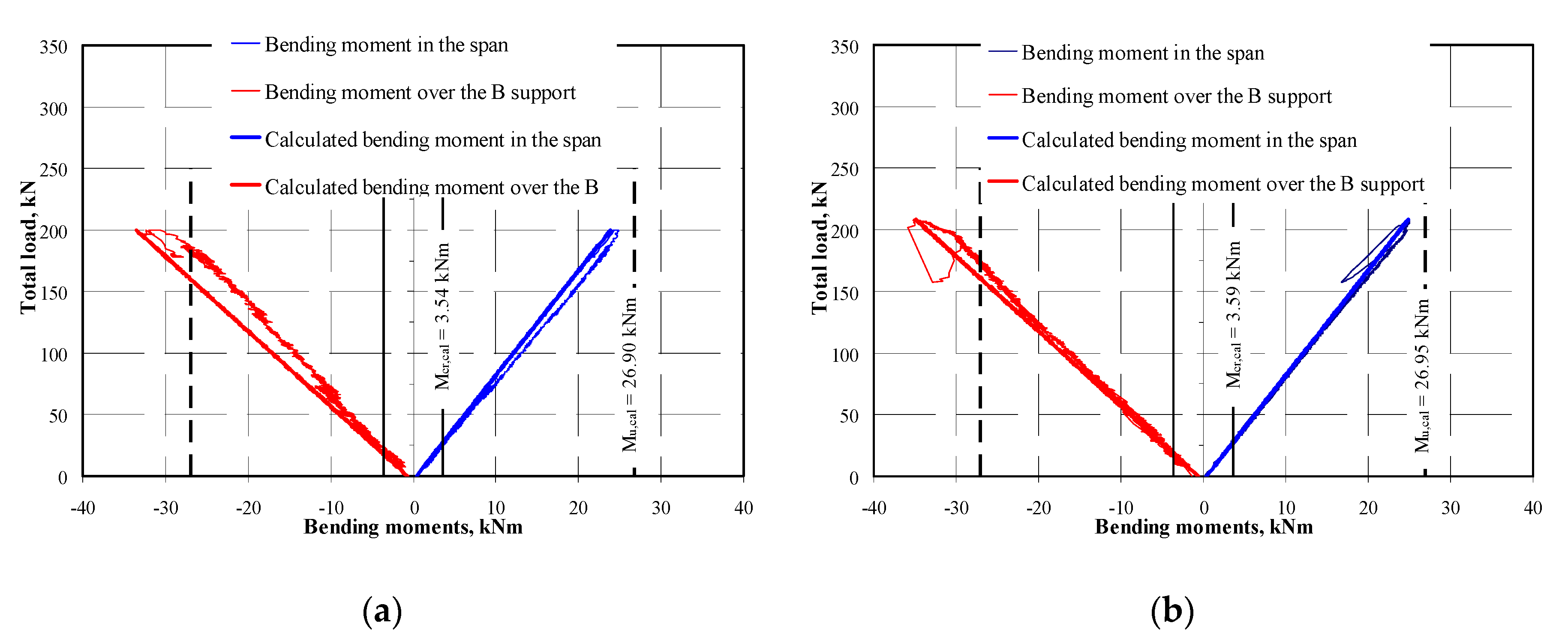
Figure 21 shows the comparison of changes in support responses that were experimentally determined or calculated from the model of an elastic continuous beam. There was no significant difference in measured and theoretical responses until cracking of the support section. At that time a small drop in response values was observed for the internal support B at simultaneously increasing response at the edge support A. A further increase in loads clearly reduced the response mechanism of the internal support and caused an increase in the response from the edge support. However, these changes were nearly proportional. At the time preceding the failure, the values of measured and calculated responses differed by no more than 10% with reference to theoretical responses. Figure 22 shows changes in bending moments in the over-support and span sections where the plastic hinge was formed. The values were experimentally determined and calculated for the model of a two-span elastic beam. For Beam No. 1, the over-support moment that was experimentally determined did not significantly differ from the theoretical value within the range of controlled force increase up to the load of 50 kN. A further increase in total load imposed by the constant increase in displacement of the actuator piston resulted in a clear drop of the moment over the support at a simultaneous increase of the span moment. At the time preceding the failure, the support moment again increased, and the span moment decreased.
Changes in values of bending moments were not so obvious in case of Beam No. 2, for which only an increase in load was controlled. The support and span moments did not differ from the calculated values until the load of 50 kN. As for Beam No. 1, a clear increase in bending moments over the support was observed at the time preceding the failure. These values were close to the theoretical ones. Table 2 presents values of total load of the span at the time of cracking of the support and the span, and at the time of failure and calculated force values taking into account plastification and redistribution of bending moments in accordance with the standard ideally plastic model. Forces inducing cracks in Beam No. 1 with a controlled increase in the force were greater by 13-15% than the calculated ones. At the time of failure, that is, at the stage of a controlled increase in displacement, the maximum load was smaller by only 2% than the calculated value. For Beam No. 2 with a controlled increase in force, the load at the time of support cracking was smaller by 10% from the calculated value, and greater by 9% at the time of span cracking. Load at the time of failure was greater by 2% than the calculated value.
At the time of failure single-sided rotations of bottom section were as follows:
Beam No. 1—0.502° = 8.76 mrad,
Beam No. 2—0.782° = 13.65 mrad.
Mutual rotations of the supports in the sections symmetrical to the support B were equal to:
Beam No. 1—Θpl,d = 2 × 8.76 = 17.5 mrad,
Beam No. 2—Θpl,d = 2 × 13.65 = 27.3 mrad.
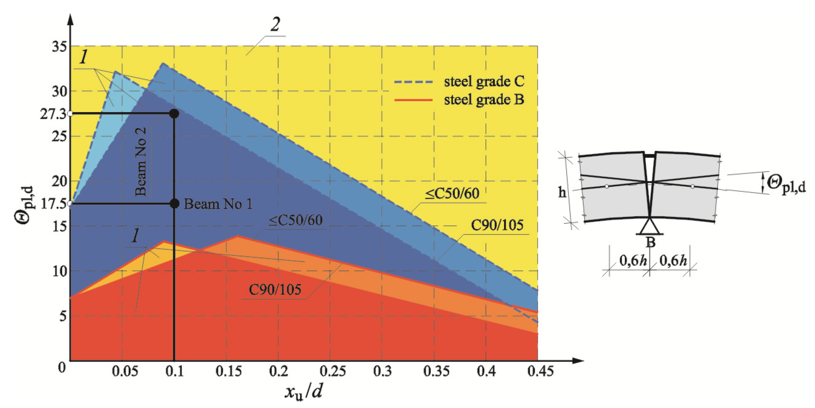
These results for concrete types with the strength fck = 49.6 N/mm2 and 51.3 N/mm2 were lower than the allowable values (at xu/d = 0.1, shown in Figure 5.6 N, the standard EN 1992-1-1:2010 [57]) equal to 32.5 mrad. Test results are shown in Figure 23. It can be presumed that the method of load control caused significant differences in values of angles of mutual rotations. In case of Beam No. 2 with controlled force P(t), the mutual rotation of the sections was over 56% greater than the rotation of Beam No. 1, in which cracking was controlled with an increase in displacement u(t).
6. Conclusions
The tests performed at the developed test stand confirmed its total suitability for testing elements and structures using different methods of controlling load. Displacements of the specific structure area were controlled in a direct way by inducing displacement of the actuator piston and non-contact recording of the span displacement. The structure displacements were successfully controlled in the initial phase of testing at the rigid stand.
The modern electrical system based on the CompactRIO controller cooperating with the ARAMIS software was used in the existing hydraulic pump. The advanced controller for a large number of high-frequency sampling signals at real time ensured very high accuracy of the measurements. Software developed in the LabView environment, which was especially intended for the test stand, provided an option of choosing load paths for a structure, whose displacements or deformations were controlled in a non-contact way. Therefore, we developed a unique test stand for testing test elements and building structures, which ensured the complete control over displacements, strains, or crack widths. This test stand obtained the features of modern testing machines using the DIC technique for measuring small samples. The existing measurement errors caused by the test stand susceptibility, clearance in structures, and accidental errors were minimized by directly measuring the structure response.
The statistically non-determinable reinforced concrete beams were used as the test elements. This type of structures highlights non-linear occurrences related to cracks in different sections and redistribution of internal forces. In case of Beam No. 1, for which an increase in load over time P(t) was controlled until the time of cracking, and then an increase in displacements was controlled over time u(t), a clear distribution of bending moments was observed. Similar results were obtained for Beam No. 2 with controlled load over time P(t). However, the redistribution of bending moments was not so obvious. As it was expected, the results were close to the values calculated in accordance with the standard procedures. There was a significant difference in case of angles of mutual rotations. For the beam with controlled force P(t), the mutual rotation of the sections was over 56% greater than rotations of sections in the beam with controlled in displacements u(t).
Mechanical clearance in frames of the test stand structures can considerably reduce the control of displacements. Therefore, this issue should be included in the control algorithm in order to eliminate the clearance impact on the control quality. This software can be further developed by adding extra hydraulic power packs to induce sequential and/or spatial loading and even cyclic one. Papers to date on remote controlling of loading have been submitted to the Polish Patent Office as the independent test stand [58].
Author Contributions
Conceptualization, R.J. and K.S.; methodology, R.J.; software, K.S. and J.D.; validation, K.S. and J.D.; formal analysis, R.J.; investigation, R.J., K.S., and J.D.; data curation, K.S.; writing—original draft preparation, R.J., K.S., and J.D.; writing—review and editing, R.J., K.S., and J.D.; visualization, R.J., K.S., and J.D.; supervision, R.J.; project administration, R.J. All authors have read and agreed to the published version of the manuscript.
Funding
The research reported in this paper was co-financed by the European Union from the European Social Fund in the framework of the project “Silesian University of Technology as a Center of Modern Education based on research and innovation” POWR.03.05.00-00-Z098/17.
Acknowledgments
Authors would like to thank students of Silesian University of Technology: Jan Biernacki, Mikołaj Koziej, Adam Porwoł, Szymon Buryan, Bartłomiej Klama, Oskar Szurkat who participated in the preparatory works and basic tests of the research stand. Special thanks go to the experts involved in the project: PhD Wociech Mazur (the ARAMIS software), PhD Jan Pizoń (technology of concrete) for their help in preparing the test elements and interpreting the results.
Conflicts of Interest
The authors declare no conflict of interest.
References
- Hernandez, B.A.; Gill, H.S.; Gheduzzi, S. A Novel Modelling Methodology Which Predicts the Structural Behaviour of Vertebral Bodies under Arial Impact Loading: A Finite Element and DIC Study. Materials 2020, 13, 4262. [Google Scholar] [CrossRef] [PubMed]
- Carvalho, L.; Roriz, P.; Simões, J.; Frazão, O. New Trends in Dental Biomechanics with Photonics Technologies. Appl. Sci. 2015, 5, 1350–1378. [Google Scholar] [CrossRef] [Green Version]
- Gamboa, C.B.; Martín-Béjar, S.; Trujillo Vilches, F.J.; Castillo López, G.; Sevilla Hurtado, L. 2D–3D Digital Image Correlation Comparative Analysis for Indentation Process. Materiale 2019, 12, 4156. [Google Scholar] [CrossRef] [PubMed] [Green Version]
- Huang, Y.H.; Liu, L.; Sham, F.C.; Chan, Y.S.; Ng, S.P. Optical strain gauge vs. traditional strain gauges for concrete elasticity modulus determination. Opt. Int. J. Light Electron Opt. 2010, 18, 1635–1641. [Google Scholar] [CrossRef]
- Romeo, E. Two-dimensional digital image correlation for asphalt mixture characterization: Interest and limitations. Road Mater. Pavement Des. 2013, 14, 747–763. [Google Scholar] [CrossRef]
- Blenkinsopp, R.; Roberts, J.; Parland, A.; Sherratt, P.; Smith, P.; Lucas, T. A Method for Calibrating a Digital Image Correlation System for Full-Field Strain Measurements during Large Deformations. Appl. Sci. 2019, 9, 2828. [Google Scholar] [CrossRef] [Green Version]
- Zhao, Y.; Taheri, A.; Soltani, A.; Karakus, M.; Deng, A. Strength Development and Strain Localization Behavior of Cemented Paste Backfills Rusing Portland Cement and Fly Ash. Materials 2019, 12, 3282. [Google Scholar] [CrossRef] [Green Version]
- Pan, K.; Yu, R.C.; Hang, X.; Ruiz, G.; Wu, Z. Propagation Speed of Dynamic Mode-I Cracks in Self-Compacting Steel Fiber-Reinforced Concrete. Materials 2020, 13, 4053. [Google Scholar] [CrossRef] [PubMed]
- Zhang, F.; Yan, G.; Yang, Q.; Gao, J.; Li, Y. Strain Field Evolution Characteristics of Free Surface during Crater Blasting in Sandstone under High Stress. Appl. Sci. 2020, 10, 6285. [Google Scholar] [CrossRef]
- Linke, M.; Flügge, F.; Olivares-Ferrer, A.J. Design and Validation of a Modified Compression-After-Impact Testing Device for Thin-Walled Composite Plater. J. Compos. Sci. 2020, 4, 126. [Google Scholar] [CrossRef]
- Kötter, B.; Karoten, J.; Körbelin, J.; Fiedler, B. CFRP Thin-Ply Fibre Metal Laminates: Influences of Ply Thickness and Metal Layers on Open Hole Tension and Compression Properties. Materials 2020, 13, 910. [Google Scholar] [CrossRef] [PubMed] [Green Version]
- Zhao, Y.; Hu, D.; Hang, M.; Dai, W.; Hang, W. In Situ Measurements for Plastic Zone Ahead of Crack Tip and Continuous Strain Variation under Cyclic Loading Using Digital Image Correlation Method. Metals 2020, 10, 273. [Google Scholar] [CrossRef] [Green Version]
- Zhan, N.; Hu, Z.; Hang, X. Experimental Investigation of Fatigue Crack Growth Behavior in Banded Structure of Pipeline Steel. Metals 2020, 10, 1193. [Google Scholar] [CrossRef]
- Carroll, J.D.; Abuzaid, W.; Lambros, J.; Sehitoglu, H. High resolution digital image correlation measurements of strain accumulation in fatigue crack growth. Int. J. Fatigue 2013, 57, 140–150. [Google Scholar] [CrossRef]
- Travelletti, J.; Delacourt, C.; Allemand, P.; Malet, J.P.; Schmittbhul, J.; Toussaint, R.; Bastard, M. Correlation of multi-temporal ground-based optical images for landslide monitoring: Application, potential and limitations. ISPRS J. Photogramm. Remote Sens. 2012, 70, 39–55. [Google Scholar] [CrossRef]
- Mazzanti, P.; Caporossi, P.; Muzi, R. Sliding Time Master Digital Image Correlation Analyses of CubeSat Images for landslide Monitoring: The Rattlesnake Hills Landslide (USA). Remote Sens. 2020, 12, 592. [Google Scholar] [CrossRef] [Green Version]
- Bozzano, F.; Mazzanti, P.; Perissin, D.; Rocca, A.; De Pari, P.; Discenza, M.E. Basin Scale Assessment of Landslides Geomorphological Setting by Advanced InSAR Analysis. Remote Sens. 2017, 9, 267. [Google Scholar] [CrossRef] [Green Version]
- Yoshida, S.; Sasaki, T. Deformation Wave Theory and Application to Optical Interferometry. Materials 2020, 13, 1363. [Google Scholar] [CrossRef] [Green Version]
- Drobiec, Ł.; Jasiński, R.; Mazur, W.; Rybarczyk, T. Numerical Verification of Interaction between Masonry with Precast Reinforced Lintel Made of AAC and Reinforced Concrete Confining Elements. Appl. Sci. 2020, 10, 5446. [Google Scholar] [CrossRef]
- Phelan, R.M. Hydraulic press. Access Sci. 2020. [Google Scholar] [CrossRef]
- Hinton, C.E. Adaptive PID Control of Dynamic Maaterials-Testing Machines Using Remembered Stiffness, Application of Automation Technology to Fatigue and Fracture Testing and Analysis: Third Volume, ASTM STP International 1303; Braun, A.A., Gilbert-Son, L.N., Eds.; American Society for Testing and Materials: West Conshohocken, PA, USA, 1997; pp. 111–119. [Google Scholar] [CrossRef]
- Bolton, W. Mechatronics Electronic Control Systems in Mechanical and Electrical Engineering; Prentice Hall: London, UK, 2009; ISBN 978-0-13-240763-2. [Google Scholar]
- Rohner, P. Industrial Hydrualic Control; Willey: Hoboken, NJ, USA, 1995; ISBN 958149313. [Google Scholar]
- Bolton, W. Pneumatic and Hydraulic Systems; Butterworth-Heinemann Ltd.: Oxford, UK, 1997; ISBN 750638362. [Google Scholar]
- Aciatore, D.G.; Histand, M.B. Introduction to Mechatronics and Measurement Systems; McGraw-Hill Companies: New York, NY, USA, 2012; ISBN 978-0072402414. [Google Scholar]
- Scholz, H. Deflection and ductility of continuous RC beams. Mag. Concr. Res. 1993, 45, 197–202. [Google Scholar] [CrossRef]
- Silva, P.F.; Ibell, T.J. Evaluation of Moment Distribution in Continuous Fiber-Reinforced Polymer-Strengthened Concrete Beams. Aci. Struct. J. 2008, 105, 729–739. [Google Scholar]
- Sveinson, T.; Dilger, W.H. Moment Redistribution in Reinforced Concrete Structures. In Progress in Structural Engineering; Grierson, D.E., Franchi, A., Riva, P., Eds.; Springer: Dordrecht, The Netherlands, 1991. [Google Scholar] [CrossRef]
- Oehlers, D.J.; Haskett, M.; Mohamed Ali, M.S.; Griffith, M.C. Moment redistribution in reinforced concrete beams. Proc. Inst. Civ. Eng. Struct. Build. 2010, 163, 165–176. [Google Scholar] [CrossRef]
- do Carmo, R.N.F.; Sérgio Lopes, S.M.R. Ductility and linear analysis with moment redistribution in reinforced high-strength concrete beams. Can. J. Civ. Eng. 2005, 32, 194–203. [Google Scholar] [CrossRef]
- Oehlers, D.J.; Ju, G.; Li, I.S.T.; Seracino, R. Moment redistribution in continuous plated RC flexural members. Part 1: Neutral axis depth approach and tests. Eng. Struct. 2004, 26, 2197–2207. [Google Scholar] [CrossRef]
- Oehlers, D.J.; Ju, G.; Li, I.S.T.; Seracino, R. Moment redistribution in continuous plated RC flexural members. Part 2: Flexural rigidity approach. Eng. Struct. 2004, 26, 2209–2218. [Google Scholar] [CrossRef]
- Aiello, M.A.; Valente, L.; Rizzo, A. Moment redistribution in continuous reinforced concrete beams strengthened with carbon-fiber-reinforced polymer laminates. Mech. Compos. Mater. 2007, 43, 453–466. [Google Scholar] [CrossRef]
- do Carmo, R.N.F.; Sérgio Lopes, S.M.R. Available plastic rotation in continuous high-strength concrete beams. Can. J. Civ. Eng. 2008, 35, 1152–1162. [Google Scholar] [CrossRef]
- do Carmo, R.N.F.; Sérgio Lopes, S.M.R. Required plastic rotation of RC beams. Proc. Inst. Civ. Eng. Struct. Build 2006, 159, 77–86. [Google Scholar] [CrossRef]
- Fung, Y.C. Foundations of Solid Mechanics; Prentice Hall Inc.: Englewood Cliffs, NJ, USA, 1965. [Google Scholar]
- Chu, T.C.; Ranson, W.F.; Sutton, M.A.; Peters, W.H. Application of digital-image-correlation techniques to experimental mechanics. Exp. Mech. 1985, 25, 232–244. [Google Scholar] [CrossRef]
- Jin, G.-C.; Bao, N.-K.; Chung, P.S. An advanced digital speckle correlation method for strain measurement and nondestructive testing. In International Conference on Experimental Mechanics: Advances and Applications; International Society for Optics and Photonics: Singapore, 1997; Volume 2921, pp. 572–577. [Google Scholar] [CrossRef]
- Ma, S.-P.; Jin, G.-C. New correlation coefficients designed for digital speckle correlation method (DSCM). Proc. Spie 2003, 5058, 25–33. [Google Scholar] [CrossRef]
- Lewis, J.P. Fast Template Matching, Vision Interface 95; Canadian Image Processing and Pattern Recognition Society: Quebec City, QC, Canada, 15–19 May 1995; pp. 120–123. [Google Scholar]
- Tan, Y.; Zhang, L.; Guo, M.; Shan, L. Investigation of the deformation properties of asphalt mixtures with DIC technique. Constr. Build. Mater. 2012, 7, 581–590. [Google Scholar] [CrossRef]
- Nocoń, W.; Polaków, G. LabVIEW Based Cooperative Design for Control System Implementation; Luo, Y., Ed.; CDVE 2011, LNCS 6874; Springer: Berlin/Heidelberg, Germany, 2011; pp. 137–140. [Google Scholar]
- Nocoń, W. On the possibility of suspended solid quantity estimation based on fractional density changes in a batch settler. Powder Technol. 2013, 235, 931–939. [Google Scholar] [CrossRef]
- Taylor, J.R. An Introduction to Error Analysis: The Study of Uncertainties in Physical Measurements; University Science Books: Sausalito, CA, USA, 1982; pp. 128–129. ISBN 0-935702-75-X. [Google Scholar]
- Harlow, R.; Dotson, C.; Thompson, R.L. Fundamentals of Dimensional Metrology, 4th ed.; Delmar Publishers: Albany, NY, USA, 2002. [Google Scholar]
- Seber, G.A.F.; Lee, A.J. Linear Regression Analysis; John Wiley & Sons Publications: Hoboken, NJ, USA, 2003. [Google Scholar] [CrossRef]
- Hryniuk, D.; Suhorukova, I.; Oliferovich, N. Adaptive smoothing and filtering in transducers. In Proceedings of the 2016 Open Conference of Electrical, Electronic and Information Sciences, (eStream 2016), Vilnius, Lithuania, 13–15 October 2016; pp. 1–4. [Google Scholar]
- Hvozdzeu, M.; Karpovich, M. Dynamic signals filtration in high level noise condition. In Mokslas—Lietuvos ateitis/Science—Future of Lithuania; Published by VGTU Press: Vilnius, Lithuania, 2020; Volume 12, pp. 1–3. ISSN 2029-2341/eISSN 2029–2252. [Google Scholar] [CrossRef]
- Morari, M.; Zafiriou, E. Robust Process Control; Prentice-Hall Inc.: Upper Saddle River, NJ, USA, 1989; ISBN1 0137821530. ISBN2 9780137821532. [Google Scholar]
- Seborg, D.E.; Edgar, T.F.; Mellichamp, D.A. Process Dynamics and Control; John Wiley & Sons: Hoboken, NJ, USA, 1989. [Google Scholar]
- Franks, R.G.; Worley, C.W. Quantitive Analysis of Cascade Control. Ind. Eng. Chem. 1956, 48, 1074–1079. [Google Scholar] [CrossRef]
- Kaya, I.; Tan, N.; Atherton, D.P. Improved Cascade Control Structure and Controller Design. In Proceedings of the 44th IEEE Conference on Decision and Control, and the European Control Conference 2005, Seville, Spain, 12–15 December 2005. [Google Scholar]
- Raja, G.L.; Ali, A. Improved tuning of cascade controllers for stable and integrating processes with time Delay. In Proceedings of the Michael Faraday IET International Summit 2015, Kolkata, India, 12–13 September 2015; pp. 1–7. [Google Scholar] [CrossRef]
- Lloyds Raja, G.; Ali, A. Design of Cascade Control Structure for Stable Processes using Method of Moments. In Proceedings of the 2nd International Conference on Power and Embedded Drive Control (ICPEDC), Chennai, Tamilnadu, India, 21–23 August 2019. [Google Scholar] [CrossRef]
- Klopot, T.; Skupin, P.; Grelewicz, P.; Czeczot, J. Practical PLC-based Implementation of Adaptive Dynamic Matrix Controller for Energy-Efficient Control of Heat Sources. IEEE Trans. Ind. Electron. 2020. [Google Scholar] [CrossRef]
- Nowak, P.; Stebel, K.; Klopot, J.; Czeczot, T.; Fratczak, M.; Laszczyk, P. Flexible function block for industrial applications of active disturbance rejection controller. Arch. Control Sci. 2018, 28, 379–400. [Google Scholar] [CrossRef]
- CEN. EN 1992-1-1:2010 Eurocode 2: Design of Concrete Structures—Part 1-1: General Rules and Rules for Buildings; CEN: Brussels, Belgium, 2010. [Google Scholar]
- Polish Patent Office. The Testing Machine for Testing the Elements and Structures. Niepodległości 188/192, 00-950, No. P. 432225, 16 December 2019. [Google Scholar]
Figure 1.
Block diagram of test stand.

Figure 2.
Graphical interpretation of deformations for selected scanning area in a 2D system of coordinates [37]: 1—scanning area, 2—scanning area after deformation, 3—pixel subimages of the structure.
Figure 2.
Graphical interpretation of deformations for selected scanning area in a 2D system of coordinates [37]: 1—scanning area, 2—scanning area after deformation, 3—pixel subimages of the structure.

Figure 3.
ARAMIS 6M system and its main components: (a) process diagram [5], (b) main measuring module—two cameras and light source, (c) calibration cross and plate1—test element, 2—calibration cross, 3—set of two cameras; 4, 5—left and right camera image prior to loading, divided into pixels and facets, 6,7—deformed facets recorded by left and right camera after loading.

Figure 4.
Scheme of hydraulic subsystem.

Figure 5.
Block diagram of electrical subsystem.

Figure 6.
Schematic diagram of displacement or load control system.

Figure 7.
Filtering pressure signal in the window of five specimens for 100 ms.

Figure 8.
Filtering of pressure signal within the window of 50 specimens for 1000 ms.

Figure 9.
Static description of control valve: (a) original, before negative feedback occurs, (b) after negative feedback and linearization.
Figure 9.
Static description of control valve: (a) original, before negative feedback occurs, (b) after negative feedback and linearization.

Figure 10.
Geometry and reinforcement of beams.

Figure 11.
Reinforced concrete elements at the test stand: (a) from the side of optical measurements, (b) from the side of making observations of cracks; 1—test element, 2—hydraulic actuator, 3—electro-resistant dynamometer, 4—steel beams for load distribution; 5—supports of the test stand.
Figure 11.
Reinforced concrete elements at the test stand: (a) from the side of optical measurements, (b) from the side of making observations of cracks; 1—test element, 2—hydraulic actuator, 3—electro-resistant dynamometer, 4—steel beams for load distribution; 5—supports of the test stand.

Figure 12.
A view of elements of the test stand for exerting load: (a) a beam with cameras from the ARAMIS system, (b) the ARAMIS system and its other elements; 1—test element, 2—hydraulic actuator, 3—the ARAMIS system, 4—hydraulic power pack.
Figure 12.
A view of elements of the test stand for exerting load: (a) a beam with cameras from the ARAMIS system, (b) the ARAMIS system and its other elements; 1—test element, 2—hydraulic actuator, 3—the ARAMIS system, 4—hydraulic power pack.

Figure 13.
Changes in bending moments in the span and over the support in statically non-determinable beam.
Figure 13.
Changes in bending moments in the span and over the support in statically non-determinable beam.

Figure 14.
Testing programme for: (a) Beam No. 1, (b) Beam No. 2; 1—response of structure.

Figure 15.
Testing programme: (a) general view of the user interface, (b) data on loading/displacement over the function of time.
Figure 15.
Testing programme: (a) general view of the user interface, (b) data on loading/displacement over the function of time.

Figure 16.
Comparison of results from structure measurements using the LVDT transducer and the DIC technique: (a) hydraulic actuators and steel cross beams were measured using the DIC technique, (b) actual results of displacements, (c) displacement results containing the correction factor.
Figure 16.
Comparison of results from structure measurements using the LVDT transducer and the DIC technique: (a) hydraulic actuators and steel cross beams were measured using the DIC technique, (b) actual results of displacements, (c) displacement results containing the correction factor.

Figure 17.
Changes in imposed load and recorded response of structure in a function of time: (a) Beam No. 1, (b) Beam No. 2.
Figure 17.
Changes in imposed load and recorded response of structure in a function of time: (a) Beam No. 1, (b) Beam No. 2.

Figure 18.
Beams at the time of failure: (a) Beam No. 1, (b) Beam No. 2.

Figure 19.
Deformations of beam sections at the time of cracking: (a) at the support section in Beam No. 1, (b) at the span section in Beam No. 1, (c) at the support section in Beam No. 2, (d) at the span section in Beam No. 2.
Figure 19.
Deformations of beam sections at the time of cracking: (a) at the support section in Beam No. 1, (b) at the span section in Beam No. 1, (c) at the support section in Beam No. 2, (d) at the span section in Beam No. 2.

Figure 20.
Rotations of bottom sections at the time of failure: (a) Beam No. 1, (b) Beam No. 2.

Figure 21.
Changes in support responses: (a) Beam No. 1, (b) Beam No. 2.

Figure 22.
Changes in bending moments of: (a) Beam No. 1, (b) Beam No. 2.

Figure 23.
Comparison of measured values for relative rotations of sections and allowable values specified in the standard EN 1992–1–1:2010 [57]; 1—allowed rotation, 2—unacceptable allowed rotation.
Figure 23.
Comparison of measured values for relative rotations of sections and allowable values specified in the standard EN 1992–1–1:2010 [57]; 1—allowed rotation, 2—unacceptable allowed rotation.


Table 1.
Test results for beams (with self-weight and equipment weight).
| Beam | Beam Self-Weight | Weight of Steel Equipment, kN | Total Load, kN | Total Bending Moment with Self-weight and Equipment Weight, kNm | ||||
|---|---|---|---|---|---|---|---|---|
| Pcr,B | Pcr,A-B | Pu,A-B | |Mcr,B| | Mcr,A-B | Mu,A-B | |||
| 1 | 3.08 | 1.96 | 20.2 | 30.0 | 199.9 | 3.44 | 4.12 | 24.7 |
| 2 | 3.03 | 16.1 | 30.1 | 208.4 | 3.135 | 4.06 | 24.9 | |
Table 2.
Comparison of calculated and experimental results.
| Beam | Test Results Total Load, kN | Calculated Results Total Load, kN | Comparison | ||||||
|---|---|---|---|---|---|---|---|---|---|
| Pcr,B | Pcr,A-B | Pu,A-B | Pcr,calB | Pcr,calA-B | Pu,calA-B | ||||
| 1 | 20.2 | 30.0 | 199.9 | 17.59 | 26.66 | 204.3 | 1.15 | 1.13 | 0.98 |
| 2 | 16.1 | 30.1 | 208.4 | 17.90 | 27.70 | 204.7 | 0.90 | 1.09 | 1.02 |
Publisher’s Note: MDPI stays neutral with regard to jurisdictional claims in published maps and institutional affiliations. |
© 2020 by the authors. Licensee MDPI, Basel, Switzerland. This article is an open access article distributed under the terms and conditions of the Creative Commons Attribution (CC BY) license (http://creativecommons.org/licenses/by/4.0/).
Share and Cite
MDPI and ACS Style
Jasiński, R.; Stebel, K.; Domin, J. Application of the DIC Technique to Remote Control of the Hydraulic Load System. Remote Sens. 2020, 12, 3667. https://0-doi-org.brum.beds.ac.uk/10.3390/rs12213667
AMA Style
Jasiński R, Stebel K, Domin J. Application of the DIC Technique to Remote Control of the Hydraulic Load System. Remote Sensing. 2020; 12(21):3667. https://0-doi-org.brum.beds.ac.uk/10.3390/rs12213667
Chicago/Turabian StyleJasiński, Radosław, Krzysztof Stebel, and Jarosław Domin. 2020. "Application of the DIC Technique to Remote Control of the Hydraulic Load System" Remote Sensing 12, no. 21: 3667. https://0-doi-org.brum.beds.ac.uk/10.3390/rs12213667
Note that from the first issue of 2016, this journal uses article numbers instead of page numbers. See further details here.