An Improved Spatiotemporal Data Fusion Method Using Surface Heterogeneity Information Based on ESTARFM

Abstract
:
1. Introduction
2. Materials
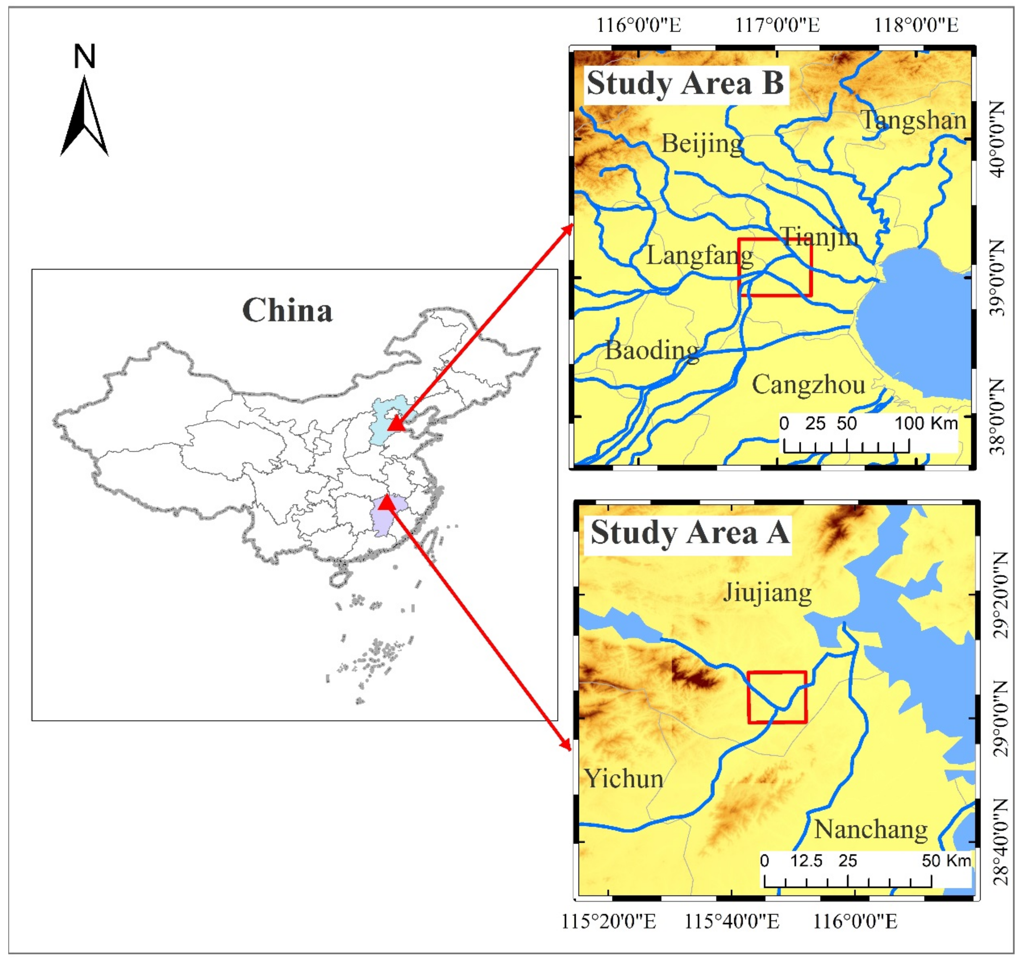
2.1. Study Area
2.2. Data
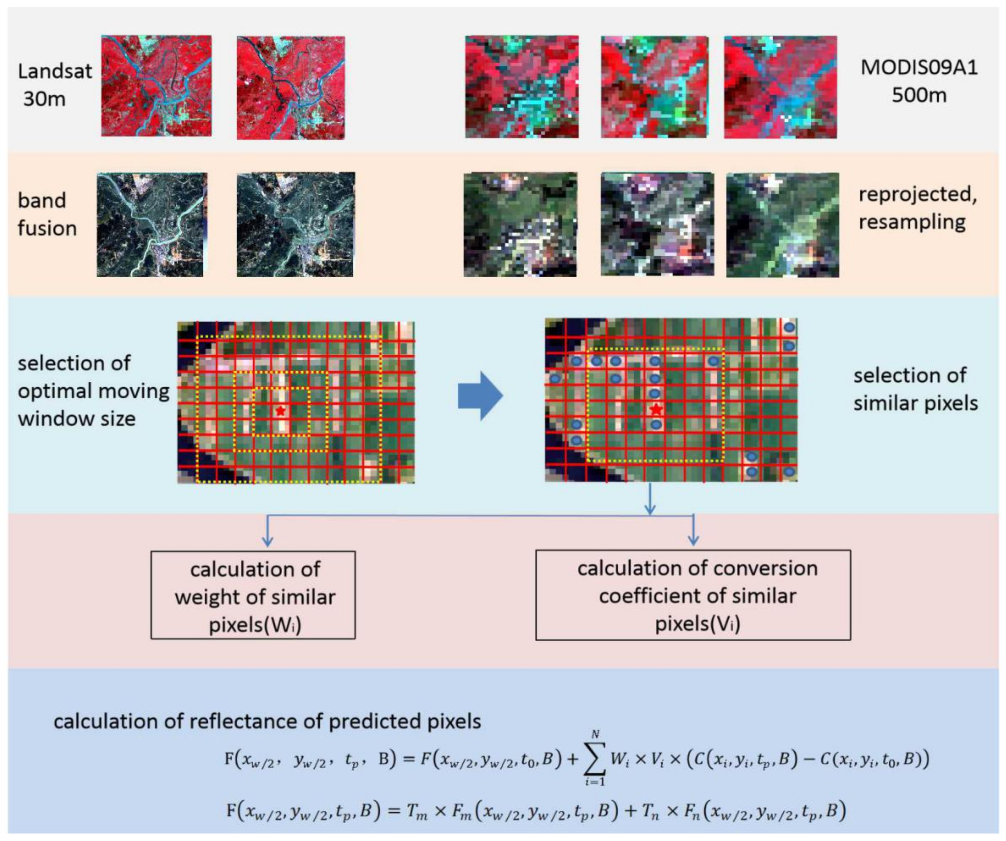
3. Method
3.1. The Overview of ESTARFM
3.2. The Proposed Methodology
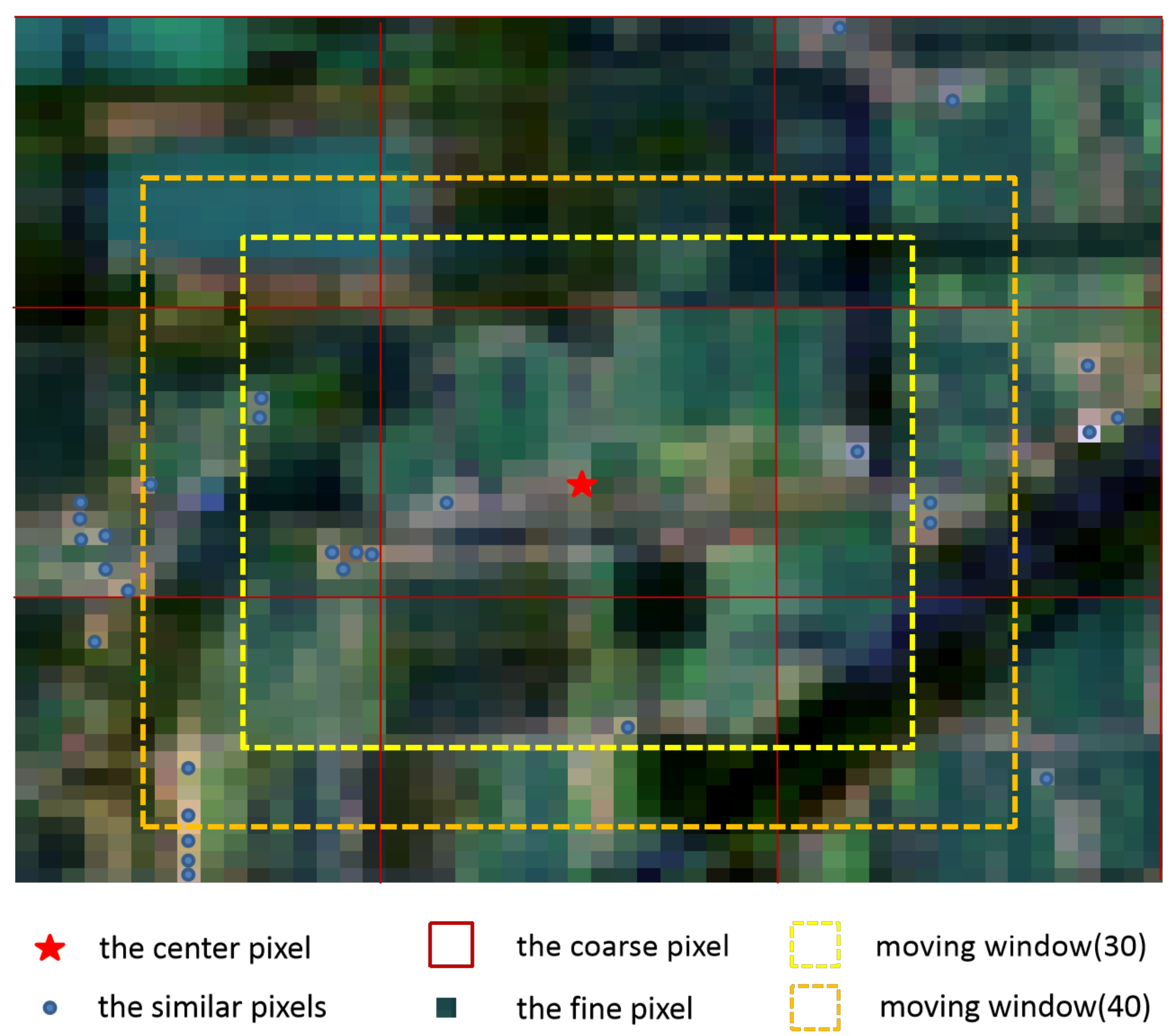
3.2.1. The Introduction of Local Variance
3.2.2. The Calculation of Local Variance within Different Moving Windows
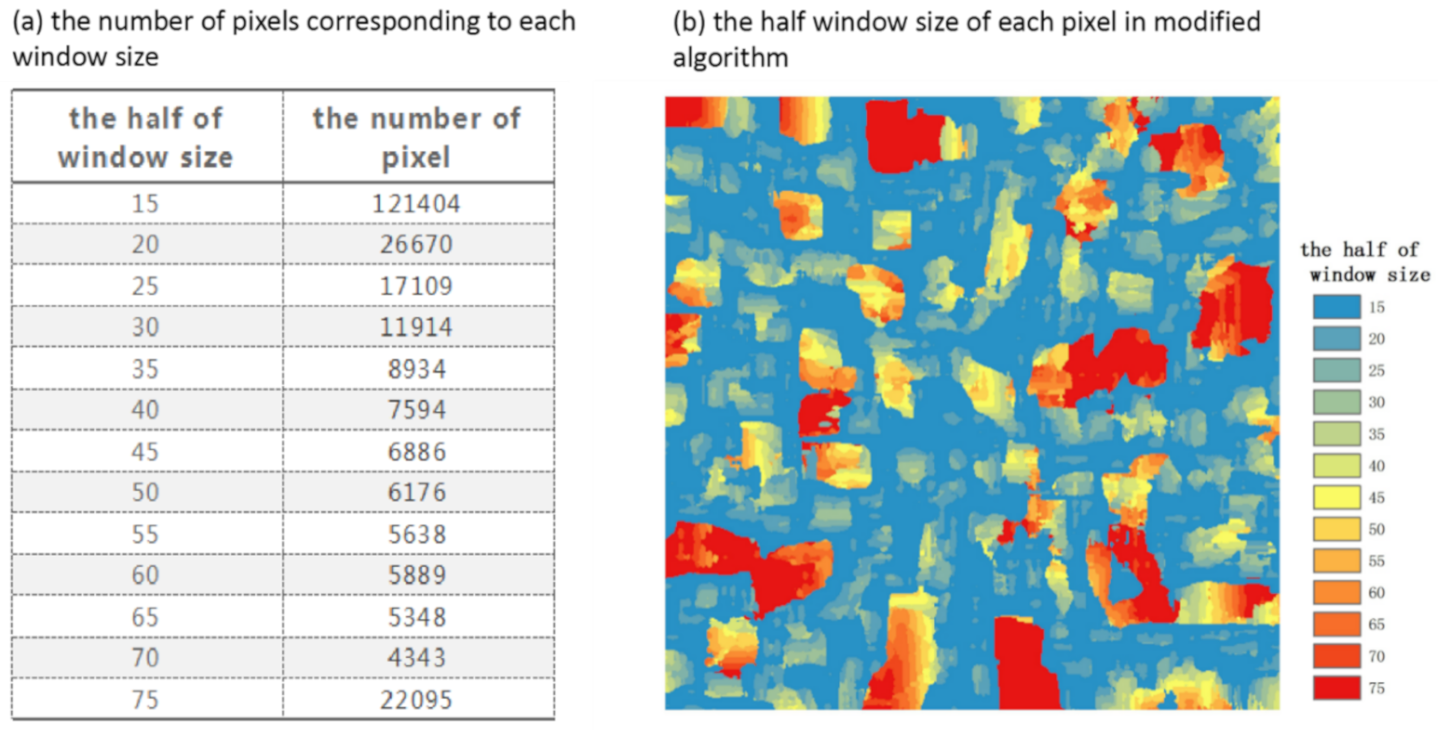
3.2.3. Carrying Out of Modified Algorithm
4. Results
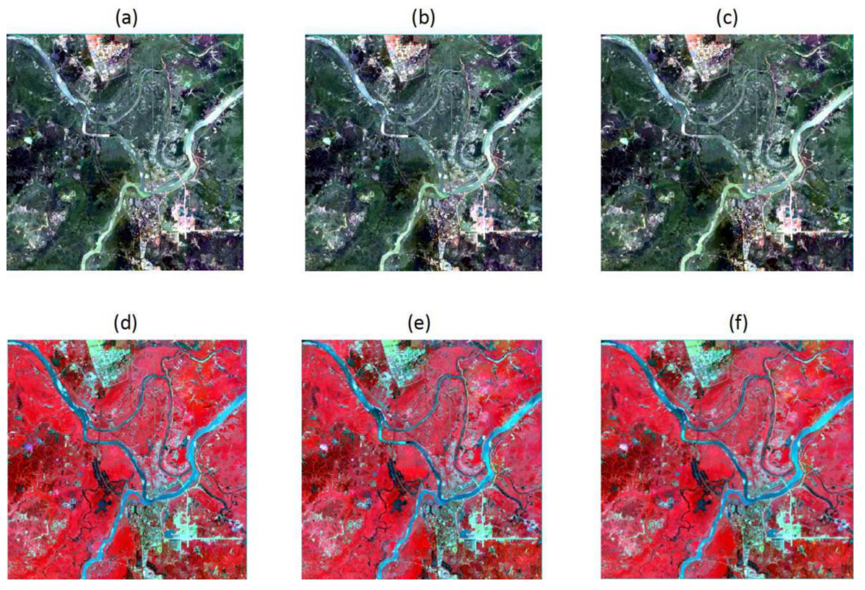
4.1. Subjective Assessment
4.2. Objective Assessment
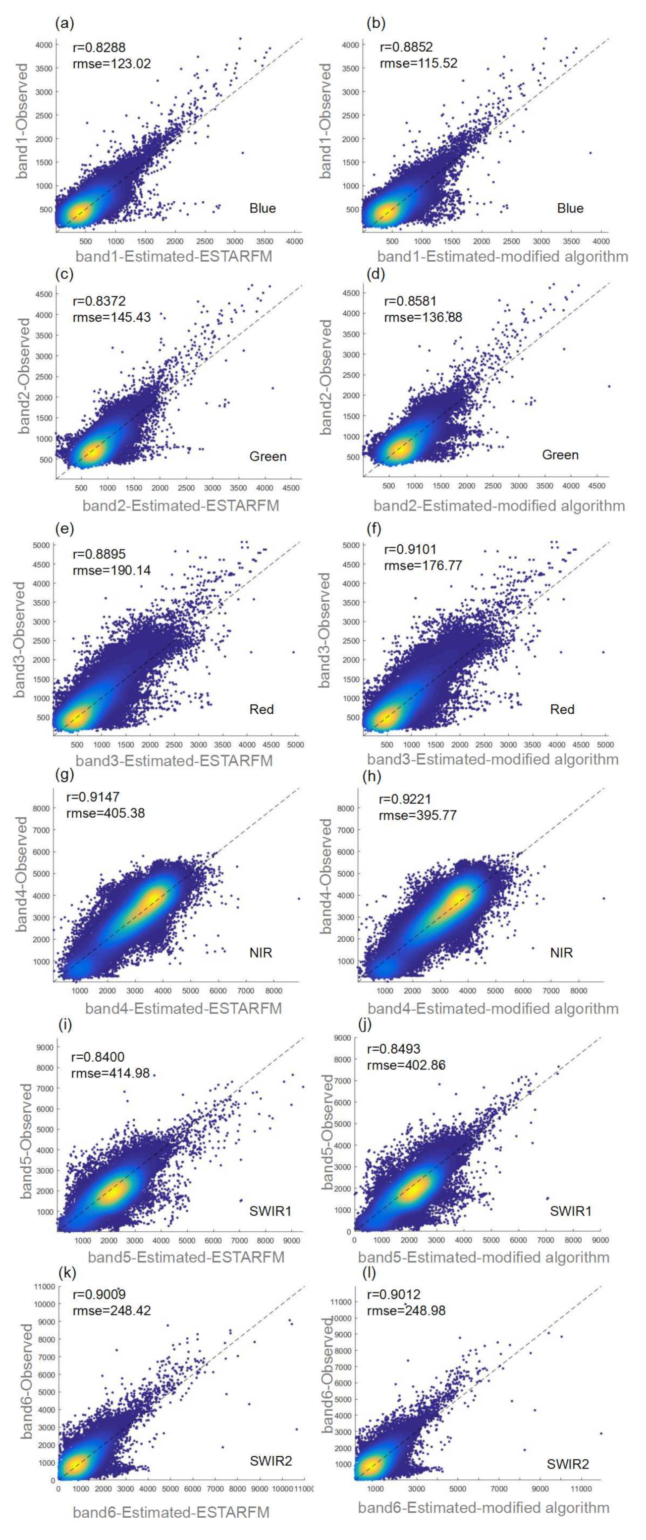
4.2.1. The Ordinary Indicator
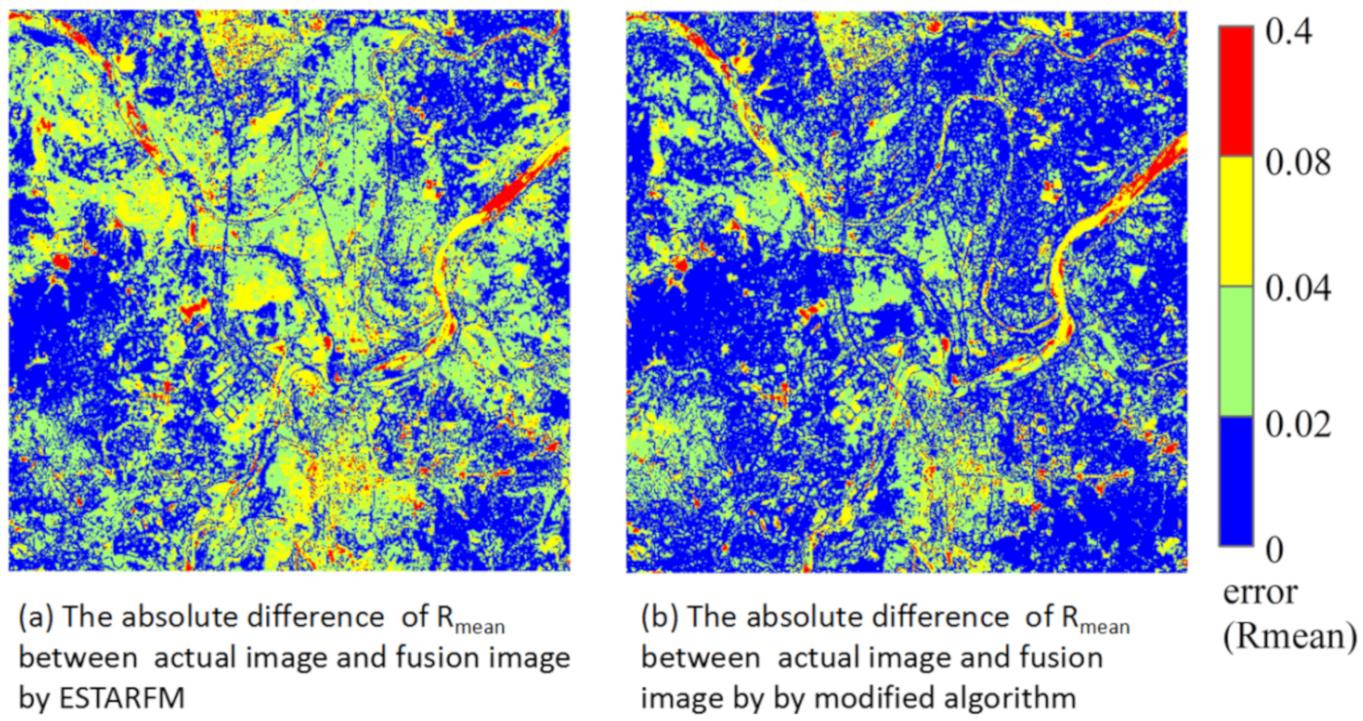
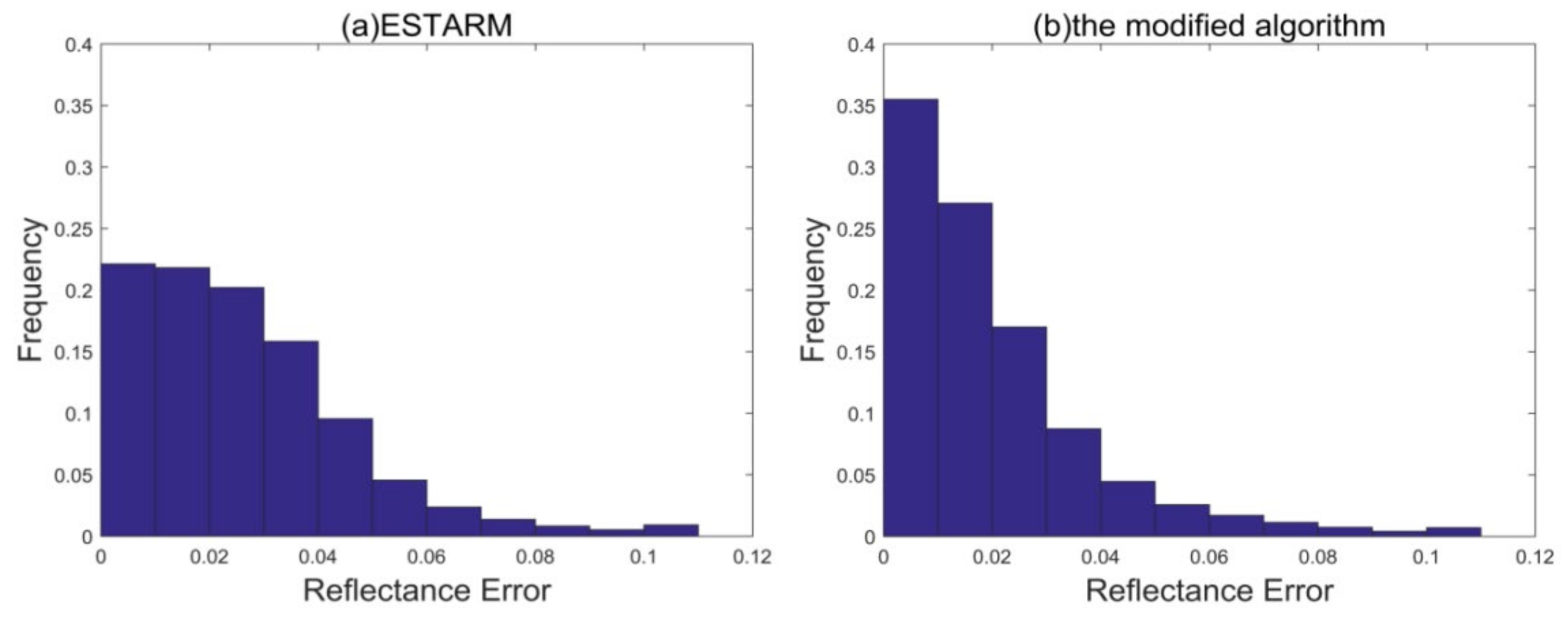
4.2.2. The Mean Difference of Six Bands
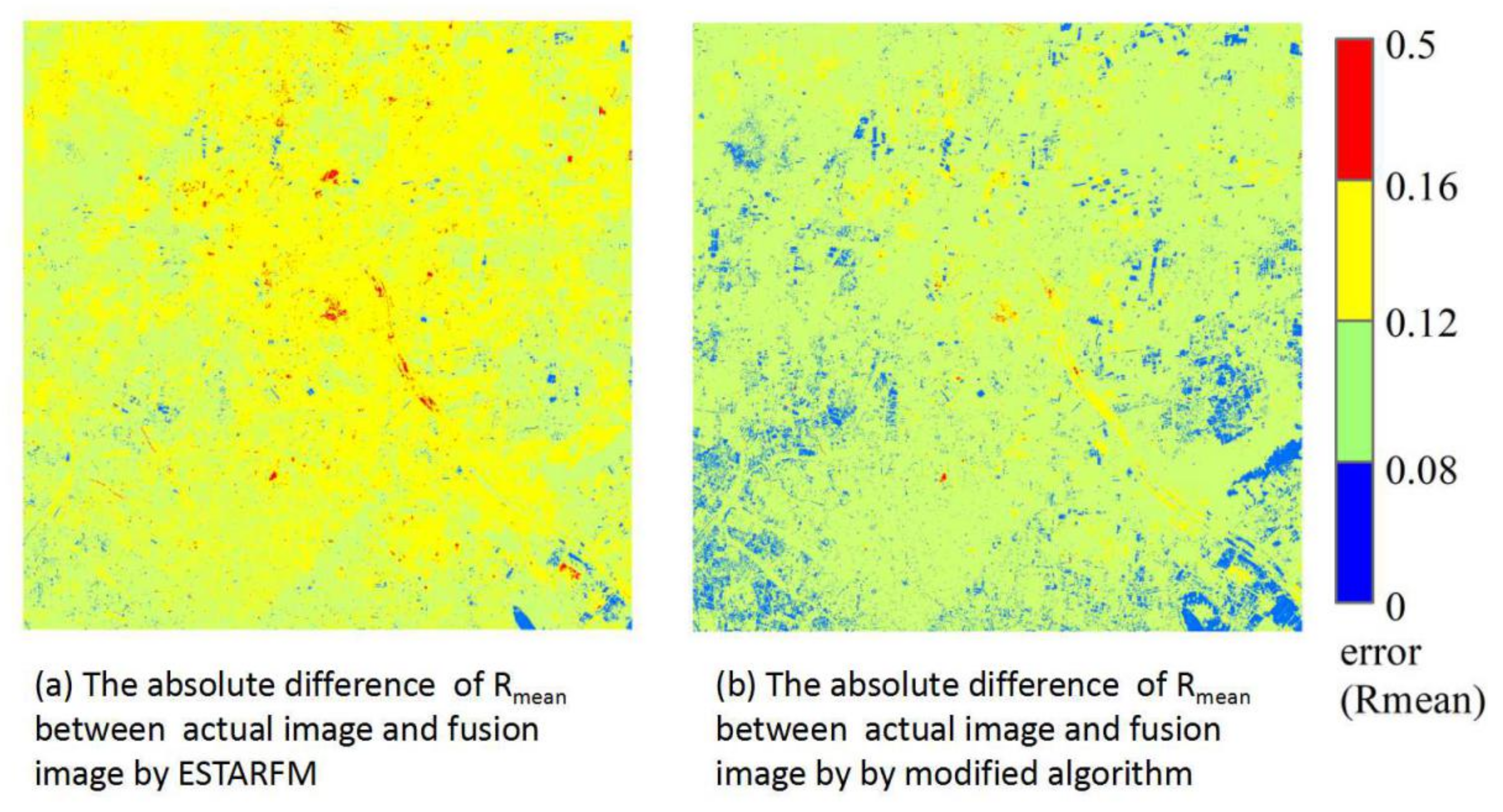
4.3. Robustness Validation
5. Discussion
6. Conclusions
Author Contributions
Funding
Acknowledgments
Conflicts of Interest
References
- Anoona, N.P.; Katpatal, Y.B. Remote sensing and gis-based analysis to envisage urban sprawl to enhance transport planning in a fast developing indian city. In Applications of Geomatics in Civil Engineering; Springer: Singapore, 2020; pp. 405–412. [Google Scholar]
- Li, S. Multisensor remote sensing image fusion using stationary wavelet transform: Effects of basis and decomposition level. Int. J. Wavelets Multiresolut. Inf. Process. 2008, 6, 37–50. [Google Scholar] [CrossRef]
- Wang, Q.; Atkinson, P.M. Spatio-temporal fusion for daily sentinel-2 images. Remote Sens. Environ. 2018, 204, 31–42. [Google Scholar] [CrossRef] [Green Version]
- Weng, Q.; Fu, P.; Gao, F. Generating daily land surface temperature at landsat resolution by fusing landsat and modis data. Remote Sens. Environ. 2014, 145, 55–67. [Google Scholar] [CrossRef]
- Zou, X.; Liu, X.; Liu, M.; Liu, M.; Zhang, B. A framework for rice heavy metal stress monitoring based on phenological phase space and temporal profile analysis. Int. J. Environ. Res. Public Health 2019, 16, 350. [Google Scholar] [CrossRef] [Green Version]
- Zhang, B.; Liu, X.; Liu, M.; Meng, Y. Detection of rice phenological variations under heavy metal stress by means of blended landsat and modis image time series. Remote Sens. 2019, 11, 13. [Google Scholar] [CrossRef] [Green Version]
- Lu, Y.; Wu, P.; Ma, X.; Li, X. Detection and prediction of land use/land cover change using spatiotemporal data fusion and the cellular automata–markov model. Environ. Monit. Assess. 2019, 191, 68. [Google Scholar] [CrossRef] [PubMed]
- Wu, P.; Shen, H.; Zhang, L.; Göttsche, F.-M. Integrated fusion of multi-scale polar-orbiting and geostationary satellite observations for the mapping of high spatial and temporal resolution land surface temperature. Remote Sens. Environ. 2015, 156, 169–181. [Google Scholar] [CrossRef]
- Zhu, X.; Cai, F.; Tian, J.; Williams, K.A. Spatiotemporal fusion of multisource remote sensing data: Literature survey, taxonomy, principles, applications, and future directions. Remote Sens. 2018, 10, 527. [Google Scholar]
- Niu, Z.; Wu, M.; Wang, C. Use of modis and landsat time series data to generate high-resolution temporal synthetic landsat data using a spatial and temporal reflectance fusion model. J. Appl. Remote Sens. 2012, 6, 63507. [Google Scholar] [CrossRef]
- Zurita-Milla, R.; Clevers, J.G.P.W.; Schdepman, M.E. Unmixing-based landsat tm and meris fr data fusion. IEEE Geosci. Remote Sens. Lett. 2008, 5, 453–457. [Google Scholar] [CrossRef] [Green Version]
- Zhang, W.; Li, A.; Jin, H.; Bian, J.; Zhang, Z.; Lei, G.; Qin, Z.; Huang, C. An enhanced spatial and temporal data fusion model for fusing landsat and modis surface reflectance to generate high temporal landsat-like data. Remote Sens. 2013, 5, 5346–5368. [Google Scholar] [CrossRef] [Green Version]
- Dongjie, F.; Baozhang, C.; Juan, W.; Xiaolin, Z.; Thomas, H. An improved image fusion approach based on enhanced spatial and temporal the adaptive reflectance fusion model. Remote Sens. 2013, 5, 6346–6360. [Google Scholar]
- Wu, B.; Huang, B.; Cao, K.; Zhuo, G. Improving spatiotemporal reflectance fusion using image inpainting and steering kernel regression techniques. Int. J. Remote Sens. 2016, 38, 706–727. [Google Scholar] [CrossRef]
- Jie, X.; Yee, L.; Tung, F. A bayesian data fusion approach to spatio-temporal fusion of remotely sensed images. Remote Sens. 2017, 9, 1310. [Google Scholar]
- Shen, H.; Meng, X.; Zhang, L. An integrated framework for the spatio–temporal–spectral fusion of remote sensing images. IEEE Trans. Geosci. Remote Sens. 2016, 54, 7135–7148. [Google Scholar] [CrossRef]
- Huang, B.; Zhang, H.; Song, H.; Wang, J.; Song, C. Unified fusion of remote-sensing imagery: Generating simultaneously high-resolution synthetic spatial–temporal–spectral earth observations. Remote Sens. Lett. 2013, 4, 561–569. [Google Scholar] [CrossRef]
- Huang, B.; Song, H. Spatiotemporal reflectance fusion via sparse representation. IEEE Trans. Geosci. Remote Sens. 2012, 50, 3707–3716. [Google Scholar] [CrossRef]
- Wu, B.; Huang, B.; Zhang, L. An error-bound-regularized sparse coding for spatiotemporal reflectance fusion. IEEE Trans. Geosci. Remote Sens. 2015, 53, 6791–6803. [Google Scholar] [CrossRef]
- Song, H.; Liu, Q.; Wang, G.; Hang, R.; Huang, B. Spatiotemporal satellite image fusion using deep convolutional neural networks. IEEE J. Sel. Top. Appl. Earth Obs. Remote Sens. 2018, 11, 821–829. [Google Scholar] [CrossRef]
- Gevaert, C.M.; García-Haro, F.J. A comparison of starfm and an unmixing-based algorithm for landsat and modis data fusion. Remote Sens. Environ. 2015, 156, 34–44. [Google Scholar] [CrossRef]
- Li, X.; Ling, F.; Foody, G.M.; Ge, Y.; Zhang, Y.; Du, Y. Generating a series of fine spatial and temporal resolution land cover maps by fusing coarse spatial resolution remotely sensed images and fine spatial resolution land cover maps. Remote Sens. Environ. 2017, 196, 293–311. [Google Scholar] [CrossRef]
- Rao, Y.; Xiaolin, Z.; Jin, C.; Jianmin, W. An improved method for producing high spatial-resolution ndvi time series datasets with multi-temporal modis ndvi data and landsat tm/etm+ images. Remote Sens. 2015, 7, 7865–7891. [Google Scholar] [CrossRef] [Green Version]
- Gao, F.; Masek, J.; Schwaller, M.; Hall, F. On the blending of the landsat and modis surface reflectance: Predicting daily landsat surface reflectance. IEEE Trans. Geosci. Remote Sens. 2006, 44, 2207–2218. [Google Scholar]
- Walker, J.J.; Beurs, K.M.D.; Wynne, R.H.; Gao, F. Evaluation of landsat and modis data fusion products for analysis of dryland forest phenology. Remote Sens. Environ. 2012, 117, 381–393. [Google Scholar] [CrossRef]
- Olsoy, P.J.; Mitchell, J.; Glenn, N.F.; Flores, A.N. Assessing a multi-platform data fusion technique in capturing spatiotemporal dynamics of heterogeneous dryland ecosystems in topographically complex terrain. Remote Sens. 2017, 9, 981. [Google Scholar] [CrossRef] [Green Version]
- Hilker, T.; Wulder, M.A.; Coops, N.C.; Seitz, N.; White, J.C.; Gao, F.; Masek, J.G.; Stenhouse, G. Generation of dense time series synthetic landsat data through data blending with modis using a spatial and temporal adaptive reflectance fusion model. Remote Sens. Environ. 2009, 113, 1988–1999. [Google Scholar] [CrossRef]
- Zhu, X.; Chen, J.; Gao, F.; Chen, X.; Masek, J.G. An enhanced spatial and temporal adaptive reflectance fusion model for complex heterogeneous regions. Remote Sens. Environ. 2010, 114, 2610–2623. [Google Scholar] [CrossRef]
- Wang, P.; Gao, F.; Masek, J.G. Operational data fusion framework for building frequent landsat-like imagery. IEEE Trans. Geosci. Remote Sens. 2014, 52, 7353–7365. [Google Scholar] [CrossRef]
- Moosavi, V.; Talebi, A.; Mokhtari, M.H.; Shamsi, S.R.F.; Niazi, Y. A wavelet-artificial intelligence fusion approach (waifa) for blending landsat and modis surface temperature. Remote Sens. Environ. 2015, 169, 243–254. [Google Scholar] [CrossRef]
- Liu, X.; Deng, C.; Chanussot, J.; Hong, D.; Zhao, B. Stfnet: A two-stream convolutional neural network for spatiotemporal image fusion. IEEE Trans. Geosci. Remote Sens. 2019, 57, 6552–6564. [Google Scholar] [CrossRef]
- Gao, F.; Hilker, T.; Zhu, X.; Anderson, M.; Masek, J.; Wang, P.; Yang, Y. Fusing landsat and modis data for vegetation monitoring. IEEE Geosci. Remote Sens. Mag. 2015, 3, 47–60. [Google Scholar] [CrossRef]
- Chen, Y.; Jian-Ping, W.U. Spatial autocorrelation analysis on local economy of three economic regions in eastern china. Sci. Surv. Mapp. 2013, 38, 89–92. [Google Scholar]
- Markham, B.L.; Storey, J.C.; Williams, D.L.; Irons, J.R. Landsat sensor performance: History and current status. IEEE Trans. Geosci. Remote Sens. 2004, 42, 2691–2694. [Google Scholar] [CrossRef]
- Carlson, T.N.; Arthur, S.T. The impact of land use—Land cover changes due to urbanization on surface microclimate and hydrology: A satellite perspective. Glob. Planet. Chang. 2000, 25, 49–65. [Google Scholar] [CrossRef]
- Ryu, J.H.; Won, J.-S.; Min, K.D. Waterline extraction from landsat tm data in a tidal flat: A case study in gomso bay, korea. Remote Sens. Environ. 2002, 83, 442–456. [Google Scholar] [CrossRef]
- Miller, H.J. Tobler’s first law and spatial analysis. Ann. Assoc. Am. Geogr. 2004, 94, 284–289. [Google Scholar] [CrossRef]
- Tobler, W.R. A computer movie simulating urban growth in the detroit region. Econ. Geogr. 1970, 46, 234. [Google Scholar] [CrossRef]
- Liu, M.; Liu, X.; Wu, L.; Zou, X.; Jiang, T.; Zhao, B. A modified spatiotemporal fusion algorithm using phenological information for predicting reflectance of paddy rice in southern china. Remote Sens. 2018, 10, 772. [Google Scholar] [CrossRef] [Green Version]
- Li, S.; Li, Z.; Gong, J. Multivariate statistical analysis of measures for assessing the quality of image fusion. Int. J. Image Data Fusion 2010, 1, 47–66. [Google Scholar] [CrossRef]
- Wang, Z.J.; Ziou, D.; Armenakis, C.; Li, D.R.; Li, Q.Q. A comparative analysis of image fusion methods. IEEE Trans. Geosci. Remote Sens. 2005, 43, 1391–1402. [Google Scholar] [CrossRef]
- Wang, Q.; Shi, W.; Li, Z.; Atkinson, P.M. Fusion of sentinel-2 images. Remote Sens. Environ. 2016, 187, 241–252. [Google Scholar] [CrossRef] [Green Version]
- Kakooei, M.; Baleghi, Y. Fusion of satellite, aircraft, and uav data for automatic disaster damage assessment. Int. J. Remote. Sens. 2017, 38, 2511–2534. [Google Scholar] [CrossRef]


| Band | Landsat7 ETM+ | Bandwidth (nm) | Landsat8 OLI | Bandwidth (nm) | MODIS | Bandwidth (nm) |
|---|---|---|---|---|---|---|
| Blue | Band 1 | 450–520 | Band 2 | 450–510 | Band 3 | 459–479 |
| Green | Band 2 | 530–610 | Band 3 | 530–590 | Band 4 | 545–565 |
| Red | Band 3 | 450–510 | Band 4 | 630–690 | Band 1 | 620–670 |
| Near Infrared (NIR) | Band 4 | 780–900 | Band 5 | 850–880 | Band 2 | 841–876 |
| Short-Wave Infrared 1 (SWIR1) | Band 5 | 1550–1750 | Band 6 | 1570–1650 | Band 6 | 1628–1652 |
| Short-Wave Infrared 2 (SWIR2) | Band 6 | 2090–2350 | Band 7 | 2110–2290 | Band 7 | 2105–2155 |
| Region | Data Type | Spatial Resolution | Path/Row | Acquisition Date | Use |
|---|---|---|---|---|---|
| Study Area A(Jiujiang) | Landsat7 ETM+ | 30 m | 122/40 | 2013/7/24 | Image fusion |
| 122/39 | 2013/8/9 | Accuracy assessment | |||
| 122/40 | 2013/9/10 | Image fusion | |||
| MOD09A1 | 500 m | h27v06 | 2013/7/20 | Image fusion | |
| 2013/8/5 | Image fusion | ||||
| 2013/9/6 | Image fusion | ||||
| Study Area B(Langfang) | Landsat8 OLI | 30 m | 2017/5/23 | Image fusion | |
| 123/32 | 2017/7/10 | Accuracy assessment | |||
| 2017/9/12 | Image fusion | ||||
| MOD09A1 | 500 m | h26v04 | 2017/5/17 | Image fusion | |
| 2017/7/4 | Image fusion | ||||
| 2017/9/6 | Image fusion |
| Reflectance | ESTARFM | The Modified Algorithm | |||||
|---|---|---|---|---|---|---|---|
| Land Cover | Band | ρ | r | RSME | ρ | r | RMSE |
| Building | Band 1 | 0.8046 | 0.7888 | 168.5 | 0.8134 | 0.7926 | 167.2 |
| Band 2 | 0.9127 | 0.8116 | 173.2 | 0.9424 | 0.8198 | 168.7 | |
| Band 3 | 0.9648 | 0.8629 | 288.1 | 1.0174 | 0.8760 | 281.9 | |
| Band 4 | 0.7791 | 0.7967 | 370.5 | 0.8184 | 0.8095 | 352.5 | |
| Band 5 | 0.8003 | 0.7945 | 421.0 | 0.8495 | 0.7974 | 409.1 | |
| Band 6 | 0.9665 | 0.8627 | 389.2 | 0.9801 | 0.8598 | 388.6 | |
| Water | Band 1 | 0.4702 | 0.6616 | 199.9 | 0.5243 | 0.6845 | 179.4 |
| Band 2 | 0.5847 | 0.7350 | 247.6 | 0.6736 | 0.7649 | 215.8 | |
| Band 3 | 0.4893 | 0.6868 | 281.7 | 0.5737 | 0.7285 | 241.1 | |
| Band 4 | 0.4060 | 0.5640 | 527.7 | 0.4282 | 0.5867 | 520.2 | |
| Band 5 | 0.1879 | 0.3362 | 548.5 | 0.2070 | 0.3607 | 541.9 | |
| Band 6 | 0.2132 | 0.3727 | 251.4 | 0.2039 | 0.3674 | 259.2 | |
| Paddy | Band 1 | 0.5554 | 0.6530 | 86.8 | 0.6335 | 0.7092 | 78.2 |
| Band 2 | 0.7055 | 0.6651 | 113.6 | 0.7727 | 0.7084 | 105.8 | |
| Band 3 | 0.7774 | 0.7306 | 120.4 | 0.8718 | 0.7863 | 105.2 | |
| Band 4 | 0.5167 | 0.5206 | 420.8 | 0.5442 | 0.5349 | 426.8 | |
| Band 5 | 0.6592 | 0.6865 | 405.2 | 0.7154 | 0.7168 | 394.4 | |
| Band 6 | 0.8072 | 0.7448 | 177.1 | 0.8036 | 0.7434 | 177.3 | |
| Non-paddy vegetation | Band 1 | 0.5211 | 0.6048 | 98.6 | 0.6088 | 0.6511 | 88.1 |
| Band 2 | 0.5443 | 0.6616 | 128.5 | 0.6097 | 0.6917 | 125.0 | |
| Band 3 | 0.6514 | 0.6739 | 138.0 | 0.7646 | 0.7339 | 121.5 | |
| Band 4 | 0.5833 | 0.6848 | 359.7 | 0.6620 | 0.7286 | 316.6 | |
| Band 5 | 0.6419 | 0.7631 | 378.2 | 0.6680 | 0.7827 | 359.8 | |
| Band 6 | 0.7698 | 0.7703 | 180.0 | 0.7872 | 0.7826 | 174.0 | |
Publisher’s Note: MDPI stays neutral with regard to jurisdictional claims in published maps and institutional affiliations. |
© 2020 by the authors. Licensee MDPI, Basel, Switzerland. This article is an open access article distributed under the terms and conditions of the Creative Commons Attribution (CC BY) license (http://creativecommons.org/licenses/by/4.0/).
Share and Cite
Liu, M.; Liu, X.; Dong, X.; Zhao, B.; Zou, X.; Wu, L.; Wei, H. An Improved Spatiotemporal Data Fusion Method Using Surface Heterogeneity Information Based on ESTARFM. Remote Sens. 2020, 12, 3673. https://0-doi-org.brum.beds.ac.uk/10.3390/rs12213673
Liu M, Liu X, Dong X, Zhao B, Zou X, Wu L, Wei H. An Improved Spatiotemporal Data Fusion Method Using Surface Heterogeneity Information Based on ESTARFM. Remote Sensing. 2020; 12(21):3673. https://0-doi-org.brum.beds.ac.uk/10.3390/rs12213673
Chicago/Turabian StyleLiu, Mengxue, Xiangnan Liu, Xiaobin Dong, Bingyu Zhao, Xinyu Zou, Ling Wu, and Hejie Wei. 2020. "An Improved Spatiotemporal Data Fusion Method Using Surface Heterogeneity Information Based on ESTARFM" Remote Sensing 12, no. 21: 3673. https://0-doi-org.brum.beds.ac.uk/10.3390/rs12213673