Ensemble of Machine-Learning Methods for Predicting Gully Erosion Susceptibility

Abstract

Gully formation through water-induced soil erosion and related to devastating land degradation is often a quasi-normal threat to human life, as it is responsible for huge loss of surface soil. Therefore, gully erosion susceptibility (GES) mapping is necessary in order to reduce the adverse effect of land degradation and diminishes this type of harmful consequences. The principle goal of the present research study is to develop GES maps for the Garhbeta I Community Development (C.D.) Block; West Bengal, India, by using a machine learning algorithm (MLA) of boosted regression tree (BRT), bagging and the ensemble of BRT-bagging with K-fold cross validation (CV) resampling techniques. The combination of the aforementioned MLAs with resampling approaches is state-of-the-art soft computing, not often used in GES evaluation. In further progress of our research work, here we used a total of 20 gully erosion conditioning factors (GECFs) and a total of 199 gully head cut points for modelling GES. The variables’ importance, which is responsible for gully erosion, was determined based on the random forest (RF) algorithm among the several GECFs used in this study. The output result of the model’s performance was validated through a receiver operating characteristics-area under curve (ROC-AUC), sensitivity, specificity, positive predictive value (PPV) and negative predictive value (NPV) statistical analysis. The predicted result shows that the ensemble of BRT-bagging is the most well fitted for GES where AUC value in K-3 fold is 0.972, whereas the value of AUC in sensitivity, specificity, PPV and NPV is 0.94, 0.93, 0.96 and 0.93, respectively, in a training dataset, and followed by the bagging and BRT model. Thus, from the predictive performance of this research study it is concluded that the ensemble of BRT-Bagging can be applied as a new approach for further studies in spatial prediction of GES. The outcome of this work can be helpful to policy makers in implementing remedial measures to minimize damages caused by gully erosion.

1. Introduction

Gully erosion is one of the major environmental problems throughout the world, especially in subtropical areas where population pressure and induced activities are severe, and vegetation can often be fairly limited and thus inadequate in protecting the soil surface from heavy rainfall due to high rate of surface runoff [1]. It is an essential aspect of soil erosion and land erosion, as well as a significant source of sediment transferred to streams that challenge the sustainable development of the world [2]. A gully is generally described as an erosional deep stream feature formed by running water with a cross-sectional area of >1 ft², which is too wide to be damaged by traditional tillage, and most often occurred in lateritic soils and comparatively in weak rocks of weathered materials [3]. This process is regulated by a combination of several important factors, including subsurface movement of water, pipe roof collapse, and overland flow [4]. While gully erosion is a consequence of natural causes, human activity may increase the evolution and development of gullies [5]. Therefore, negative consequences of gully erosion include crop damage due to sand splay [6], inundation of low lying regions [7,8,9], increased badland topography due to severe soil erosion [10]; [11,12,13], increased turbidity, lack of water storage capacity in reservoirs, food scarcity due to gradually decreasing land fertility [5], loss of life and biodiversity, and damage to infrastructure such as roads and rail [14]. As a result, several bivariate and multivariate statistical methods have been used, with the collaboration of remotely sensed satellite data, and the processing and analysis of them in a Geographic Information System (GIS) platform to determine the gully erosion susceptibility (GES), such as logistic regression [15], frequency ratio [14], weights-of-evidence [16], and evidential belief function [17]. Recently, several machine-learning algorithms (MLAs) have been widely used for prediction of GES with high accuracy such as random forest [18], support vector machine [19], artificial neural networks [20], maximum entropy approaches [21], general linear models [22], and deep learning neural networks [23]. Several gully erosion control factors responsible for the occurrence and development of gully erosion were also used in this research study for sustainable analysis of gully susceptibility assessment [16]. Several research works have also been undertaken on soil erosion assessment by applying the genetic programming method with the combination of MLAs for the estimation of vegetation cover and associated phenomena on control of soil erosion and land degradation [24,25,26]. The formation and gradual development of gully features and associated erosion is a vulnerability for land surfaces, which are deeply influenced by existing geological, climatic, hydrological, environmental and topographical factors [5,15,17,18,20]. However, several empirical data models have been found to be inaccurate in assessing regions susceptible to gully erosion. A drawback of such methods is that there are a lack of reliable data for the calculation of the collapse of the gully [27]. Established literature suggests that numerous computational methods, such as bivariate and multivariate statistical techniques, have been documented to be effective in modeling GES utilizing relevant triggering parameters and the prevalent nature of gullies for assessment and model validation [1,13,15,28]. Furthermore, considering the documented establishment and use of these methods in GES prediction, there has been a controversy on the best approach for estimating gully erosion according to its fundamentally dynamic existence. The machine-learning approach was extensively used in research studies, relevant to ecological and environmental modelling. It has been proposed that these approaches do better than other data-driven and statistical methods [29]. Literature shows that numerous research work has been carried out by using boosted regression tree (BRT) and bagging MLA separately on GES assessment by Arabameri et al. [30,31], Zabihi et al. [32], Nhu et al. [33]. In general, assessment and prediction of gully erosion with utmost accuracy is even more difficult. Keeping in view the above fact here we used BRT, bagging and a novel ensemble of BRT-bagging model for sustainable prediction of gully erosion. In this research study of GES assessment, the reason behind the selection of the aforementioned MLAs is due to their unique advantages in prediction analysis. BRT is a state-of-the-art MLA which has the capability of high prediction evaluation with the importance of ranking of input variables accordingly by using boosting techniques. On the other hand, the bagging ensemble has been used to create a classifier between multiple classifiers using a bootstrap aggregating training dataset within the model. The ensemble of any statistical and MLA has always given better performance than any single models. Therefore, in this study we also applied an ensemble of the BRT-bagging approach for better prediction of GES assessment than the single BRT and bagging model. While statistical and machine-learning methods both have their unique own benefits, studies related to GES modeling for machine-learning approaches are new, emerging and popular in academia. Therefore, the aforementioned MLAs have the capacity to fulfill a gap in this research to identify accurate gully locations in the Garhbeta- I community development (CD) Block. Keeping this in mind, this study aimed at assessing susceptibility to gully erosion and thus the relative importance of variable control using three recent ML methods i.e., BRT, bagging and BRT-bagging, respectively, and employing k-fold cross validation resampling techniques. The novelty in this research study is the ensemble approach of the BRT and bagging models. In general, the performance of a single BRT and bagging approach has been improved by using ensemble of aforementioned MLAs. Therefore, based on our knowledge and an intensive literature survey it is said that there is no research work on GES assessment by using the ensemble of BRT-bagging. As a result, the proposed ensemble approach has improved the prediction accuracy of GES and this is the novelty of this research study. The inter comparison of these models was conducted in order to choose the appropriate machine-learning algorithm (MLA) for the identification of gully locations as well as the gully erosion sensitivity analyses. The objectives of this research were: (1) identification of gully erosion contributing parameters and related multi-collinearity analysis; (2) to estimate the importance value of each variables using MLAs; (3) to examine the implications of four resampling methods of K-fold (1, 2, 3 and 4) cross validation (CV) on the efficiency of the machine learning models; (4) to predict the GES maps with maximum possible accuracy using MLAs; (5) and finally model validation using the receiver operating characteristics (ROC) curves and other statistical analysis. Consequently, GES maps prepared based on this novel ensemble method can help the environmentalist and planners to take appropriate measurements for mitigation of the fragile losses of soil and land degradation within this study area.

2. Materials and Methods

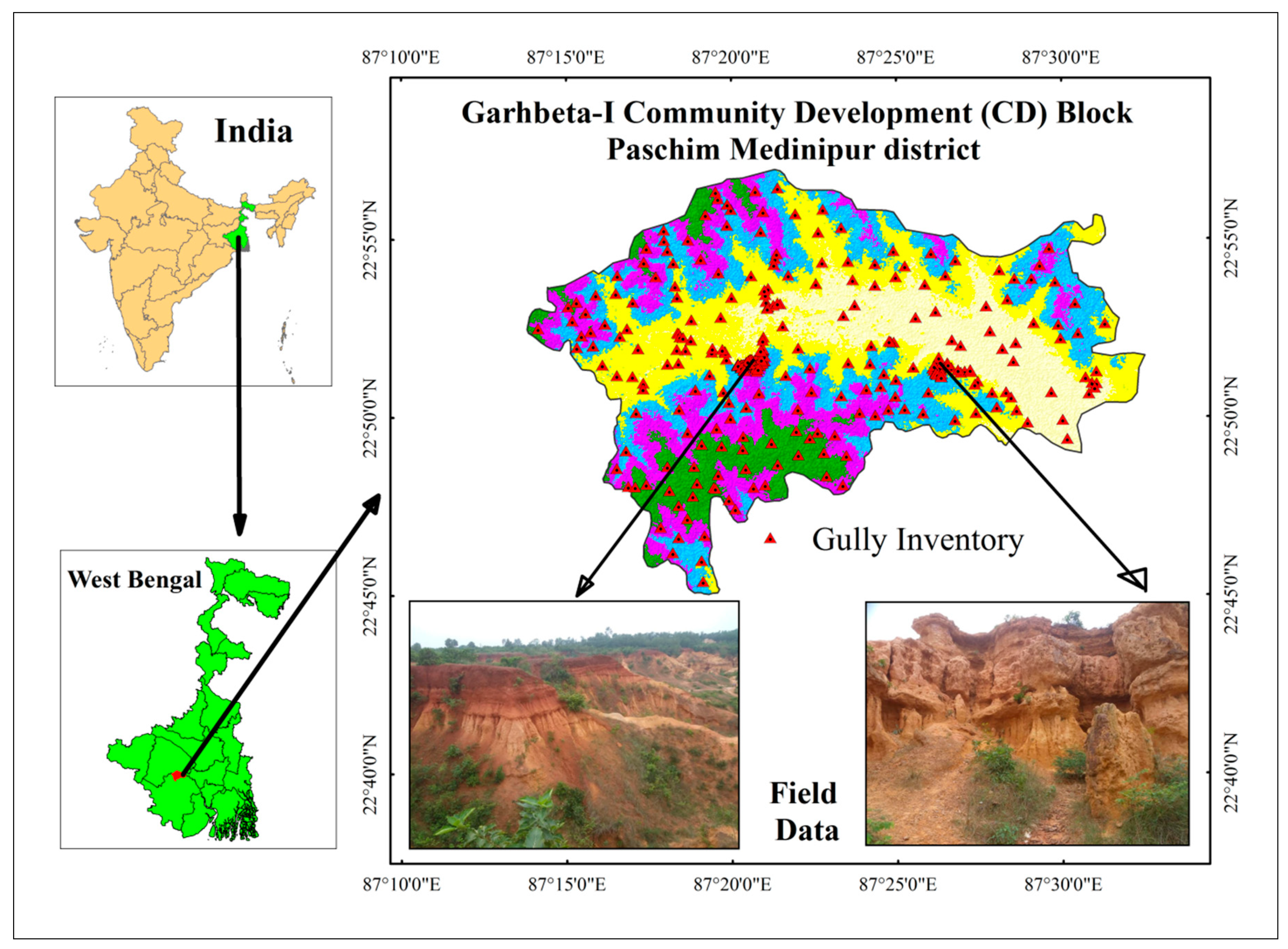
2.1. Description of the Study Area

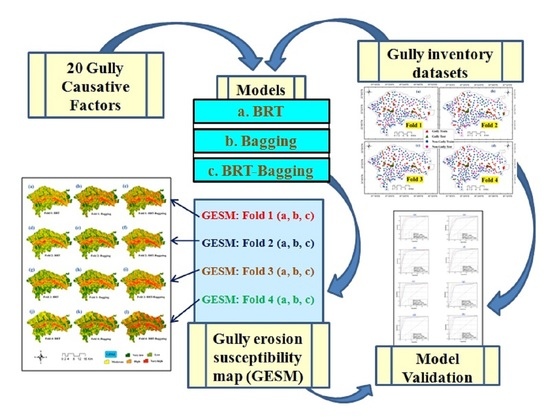
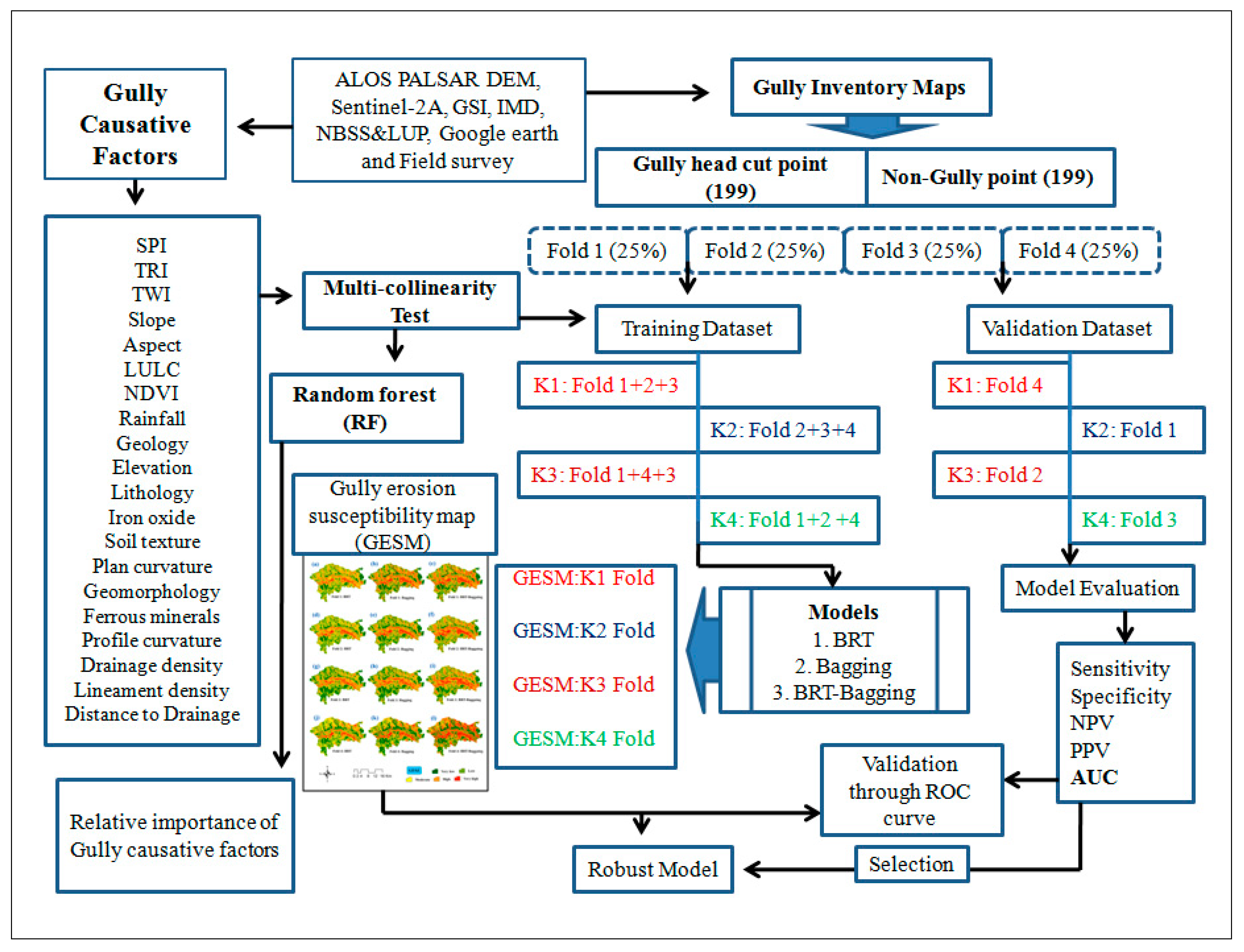
The current research study was carried out in the Garhbeta I C.D. Block of Paschim Medinipur district in West Bengal, India. The latitudinal extension of this study area is lying between 22°45′48′′N to 22°56′46′′N latitude and 87°13′17′′E to 87°32′12′′E longitude with an aerial coverage of 357.78 sq. km (Figure 1). This study area is an extended part of the Chhotanagpur plateau, and in West Bengal this extended part is known as ‘Rarh Bengal’ region. The climate of this study area is tropical monsoon type with hot-dry summer season and maximum precipitation occurring in the monsoon season i.e., in the months of July to September. The mean monthly temperature in the winter and summer season are 8 °C and 43 °C respectively, and mean annual temperature is 28 °C, with 1450 mm mean annual rainfall [34]. Therefore, this typical humid climatic region is very much prone to erosional activities through gully formation and development [35]. The main river in this study area is Shilabati (locally known as Shilai), which flows in the middle of this C.D. Block. The characteristics of land surface in this area are barren lateritic surface, hard-rocky uplands with non-arable lands. Within this C.D. Block, Garhbeta badland is the most rigorously affected by gully formation and associated land degradation problems. This Garhbeta badland is locally known as Ganganir Danga i.e., the ‘land of fires’, which is an active riverine process of gully erosion activities.

2.2. Methodology

In order to provide accurate and detailed locations of gully erosion, exhaustive field study was performed in this area and the location of gullies was registered using the Global Positioning System (GPS) instrument and verified by Google Earth satellite images. A total of 398 gully head-cut points (199 head-cut points for each gully and non-gully respectively) were selected throughout the study area. Apart from this, multi-collinearity measures through the methods of variance inflation factor (VIF) and tolerance (TOL) were employed to identify GES factors accurately. A total of 20 conditioning parameters i.e., slope, aspect, elevation, profile curvature, plan curvature, topographic wetness index (TWI), stream power index (SPI), terrain ruggedness index (TRI), rainfall, drainage density, distance to drainage, geomorphology, land use land cover (LULC), Normalized Vegetation Difference Index (NDVI), ferrous minerals, iron oxide, soil texture, geology, lineament density and lithology were chosen for predicting precise GES maps. In this study, we have chosen the non-parametric statistical method of random forest (RF) algorithm for establishing the relationship between gully head cut points and its relation with several conditioning factors. GES maps were first developed by using a boosted regression tree (BRT) and then bagging approach. Eventually, the BRT-bagging ensemble was used to develop the final GES maps. Methods of K4-fold cross validation (CV) resampling techniques have been utilized for splitting the gully head cut points. While, unlike empirical sampling distributions, they do not solve all inferential troubles, they will help generate new statistics and bring robustness to other conventional ones [36]. Cross-validation is a method of resampling that is sometimes used to determine the appropriateness of a mathematical model. The concept is to break the data arbitrarily into one set to match the algorithm, and a different set to test the model’s precision for prediction [36]. The maps of susceptibility to gully erosion are classified into five classes: very low, low, medium, high and very high using Jenk’s natural-break classification method in the ArcGIS platform. The detailed methodology flow chart of the present study area is shown in Figure 2.

2.2.1. Gully Erosion Inventory Map (GEIM)

For the modelling of GES, a gully erosion inventory map (GEIM) is necessary to understand the spatial pattern and geometrical form of gullies. In general, a GEIM is prepared based on the historical gully points and randomly selected the same number of gully points throughout the study area, for the purpose of validation of the model. GEIM also assess the relationship between the pattern and distribution of gully head-cuts and several casual factors for occurrences of gullies. In this study, a rigorous field survey was conducted to identify areas prone to gully erosion. Here, the position of each gully was measured using the Garmin (76 CSX Garmin) GPS and verified by Google Earth images. The polygon shape of the gully erosion sites was eventually converted into gully points and was used to develop a GES model. Here, we used 199 registered gully points and 199 non-gully points, and splitting them into four K-fold CV. Each fold consists of 25% of data. In this study, each time 75% data were used for training and the remaining 25% data were used for validation of GES models. In the present study area of Garhbeta I C.D. Block, GEIMs were prepared by using four K-fold CV i.e., Fold-1, Fold-2, Fold-3 and Fold-4, which is shown in Figure 3.

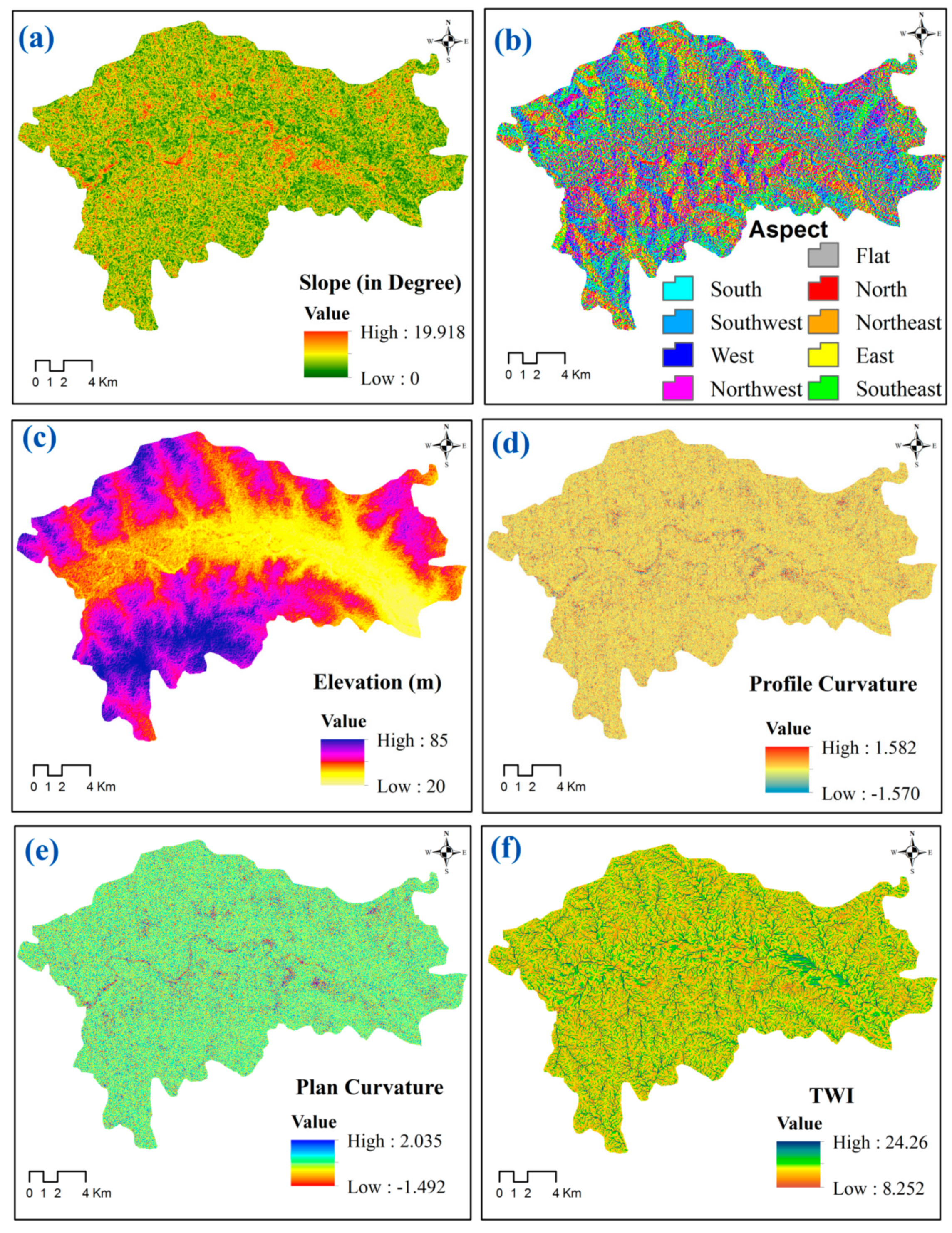
2.2.2. Dataset Preparation

For preparation of GES mapping it is indeed necessary to select suitable conditioning factors, which is responsible for their formation and development [37]. Therefore, several conditioning factors were selected based on local topographical, hydrological, climatological and geomorphological conditions within this study area. Based on the aforementioned four conditions here we selected 20 gully erosion conditioning factors (GECFs) for evaluation of GES mapping. These factors were slope, aspect, elevation, profile curvature, plan curvature, TWI, SPI, TRI, rainfall, drainage density, distance to drainage, geomorphology, LULC, NDVI, ferrous minerals, iron oxide, soil texture, geology, lineament density and lithology (Figure 4a–t). An Advanced land observing satellite (ALOS) Phased array L-band synthetic aperture radar (PALSAR) digital elevation model (DEM) with a spatial resolution of 12.5 m was also downloaded from the Alaska Satellite Facility (asf.alaska.edu) website to examine the position of each gully erosion prone areas in this study region. Several topographical indices such as slope, plan curvature, profile curvature, elevation, aspect, distance to drainage etc. were prepared by using DEM data. The soil samples were obtained randomly from the field, in order to examine the percentage wise distribution of sand, silt and clay in the study region using digital sieve shaker and digital balance machine and verified it through National Bureau of Soil Survey and Land Use Planning (NBSS&LUP) soil report. Here, the land use map was developed on the basis of the maximum likelihood method in the ERDAS imagine software based on Landsat 8 Operational land imager (OLI) satellite imagery obtained on 28/01/2020. The NDVI derived from Sentinel 2A satellite data. Geology and lithology map were obtained from the Geological Survey of India (GSI). Rainfall data of peak monsoon season (July to September) was collected from the India Meteorological Department (IMD). In fact, all of these layers and maps have been processing and annotated on the ArcGIS platform. The details of several geo-environmental factors used in this study area were categorized into following factors.

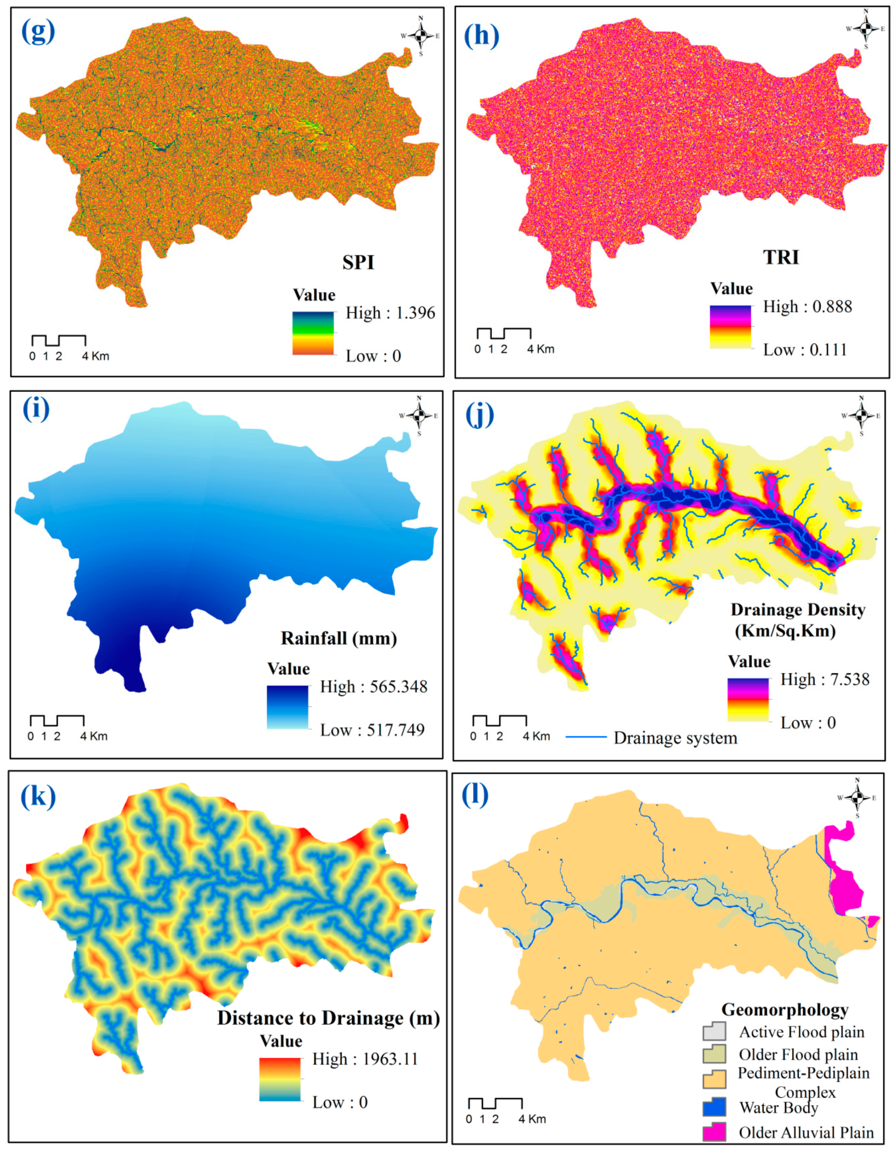
Topographical Factors

Different topographical features have a direct impact on the hydrological response of excessive runoff and these phenomena focus on the formation and development of gullies [38,39]. Alongside this, topographic features largely control the drainage network, water flow velocity and associated erosive power. In this study, six types of topographical factors were used for GES assessment and these were slope, aspect, elevation, profile curvature, plan curvature and TRI. The following equation has been used for calculating TRI values.

$$TRI=\sqrt{\left|\mathrm{X}\right|(ma{x}^2-mi{n}^2)}$$

(1)

where, X indicates altitude of every neighbor cell to a definite cell, and max and min are the highest and smallest altitude among various neighboring cell.

Hydrological Factors

The amount of surface runoff, its relation to the drainage network and erosional activities have been largely determined by hydrological influenced various conditioning factors [40]. Here, we have used five hydrological factors, namely TWI, SPI, rainfall, drainage density and distance to drainage. The following equation has been widely used for calculating TWI and SPI.

$$TWI=lo{g}_e\left(\frac{A_s}{tan\beta }\right)$$

(2)

$$SPI=A_s\ast tan\beta$$

(3)

where, $A_s$ represents the catchment area in m² and β is the gradient of the slope in radians.

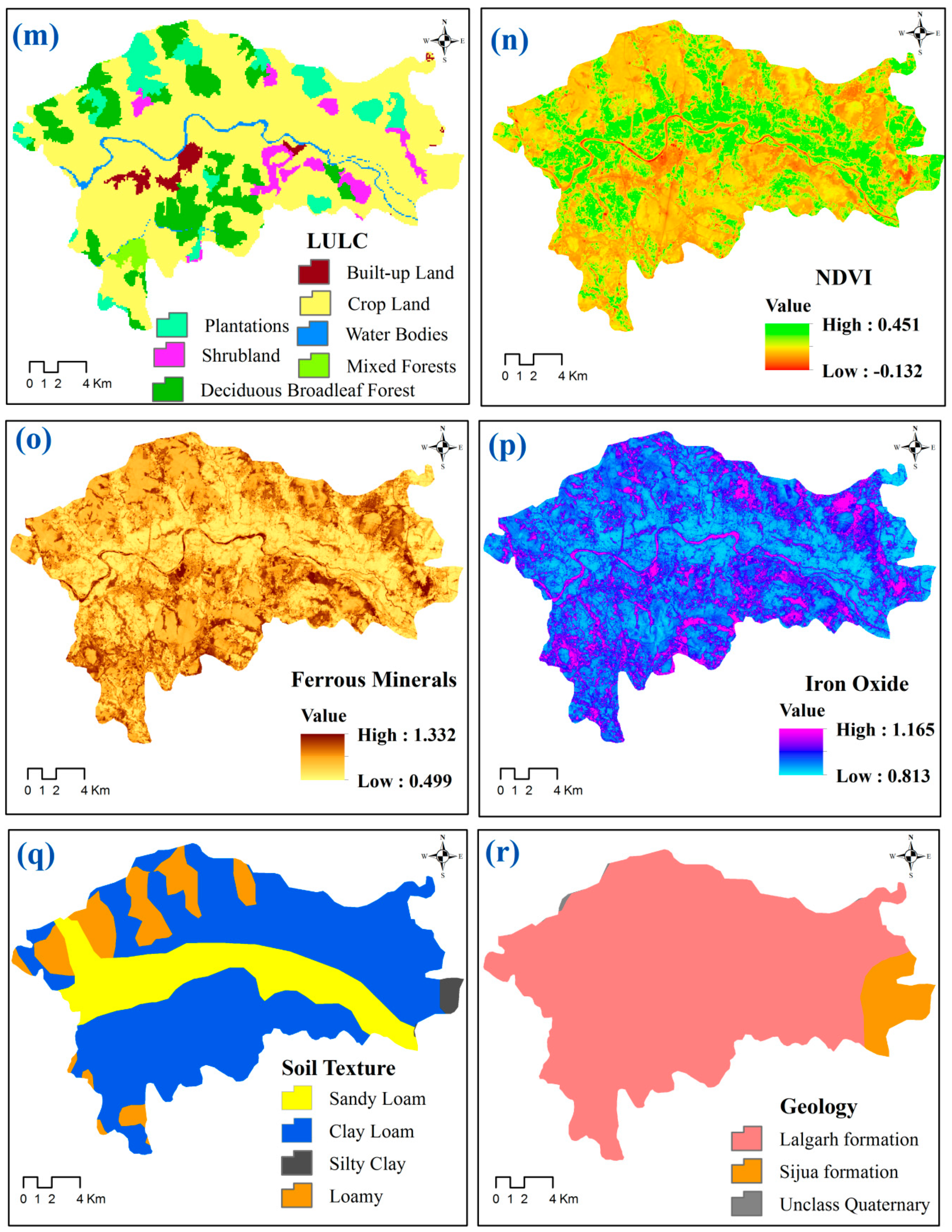
Soil-Related Factors

Water-induced soil erosion is the main cause of the formation and enlargement of gullies. Therefore, several soil characteristics are very much responsible for occurrences of gullies and land degradation. In this study, we have used soil texture, ferrous minerals and iron oxide as soil-related factors for assessment of GES mapping. Landsat 8 OLI satellite images have been used for estimation of ferrous minerals (FMI) and iron oxide by using the following equations.

$$\mathit{FMI}=\frac{\mathit{SWIR}}{\mathit{NIR}}$$

(4)

$$\mathit{Iron} \mathit{oxide}=\frac{\mathit{Red} \mathit{band}}{\mathit{Blue} \mathit{band}}$$

(5)

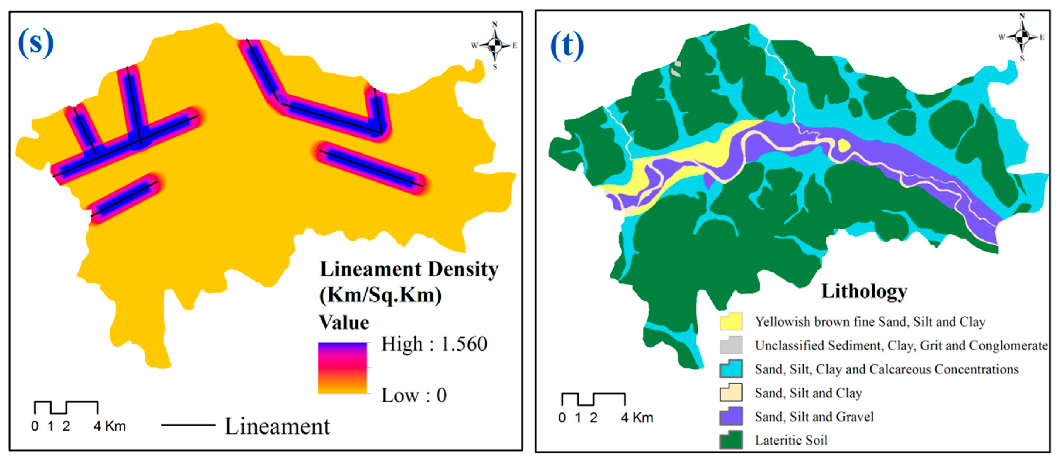
Lithological Factors

The initiation of gully erosion is very much dependent on the types of rock formation of respective rock units [20]. Here, we have used four lithological factors namely geomorphology, lithology, geology and lineament density for mapping and evaluation of gully erosion. Lineament density map was prepared on Geometica software by using Landsat 8 OLI satellite image.

Environmental Factors

The type and pattern of gully erosion is significantly determined by environmental factors. In this study, LULC and NDVI were chosen as environmental factors for GES assessment. The following equation has been used for calculating NDVI values.

$$NDVI=\frac{{\rho }_{NIR}-{\rho }_R}{{\rho }_{NIR}+{\rho }_R}$$

(6)

2.2.3. Multicollinearity Analysis

The multi-collinearity problem among the gully erosion conditioning variables is essential to recognize their susceptibility prediction power and can be displayed explicitly using the two most popular statistical techniques i.e., TOL and VIF rather than the traditional one. In this regard, the result of traditional pair correlation is ambiguity as it is not handling a big data size, is also very much affected by extreme values and result is misinterpreted when data are homogeneous. Therefore, keeping in view the above, the variance inflation factor (VIF) is taken into account as the second function of multi-collinearity analysis resulting from the Tolerance (reciprocal VIF) since that is the main measure [18]. The advantages of using VIF techniques over the traditional pair correlation is that VIF has the capacity to analysis more data and significantly reduced the standard errors, reduced correlation through recode the predictors and give a better result as predictors are less correlated among the other variables. Taking into consideration that VIF is less than 10 (less than 5 considered for weaker models) and TOL is less than 0.1 does not suggest a multi-collinearity issue and is suitable for further application in terms of analysis [17,41,42].Tolerance and VIF formulas are as follows:

$$TOL=1-R_j^2$$

(7)

$$VIF=\frac{1}{TOL}$$

(8)

where, $R_j^2$ represents the regression coefficient of determination of explanatory variable J on all the other explanatory variables.

2.2.4. Measuring the Variables’ Importance

In this research work, the importance of variables was determined by using the RF algorithm. Identification of variables importance is a significant task and measures of these variables through normal statistical techniques is not suitable due to huge data size. Therefore, in this study, we have used machine learning algorithm of RF for accurate identification of several variables importance. RF is an ensemble-based machine-learning classifier method proposed by Breiman [43]. The function of RF is based on decision trees in its initial stage of the model with the collective action of bagging approach. To identification of variables importance here we used mean decrease accuracy (MDA) index in the RF algorithm. The MDA index was calculated by using the following equation [44].

$$V{I}_j=\frac{1}{ntree}{\displaystyle \sum _{t=1}^{ntree}}E{P}_{tj}-E_{tj}$$

(9)

where, $VI$ is the variables importance, $E_{tj}$ represents the OOB error on tree t before permuting the values of $X_j$ and $E{P}_{tj}$ indicates the OOB error on tree t after permuting the values of $X_j.$

2.2.5. Machine-Learning Methods

Boosted Regression Tree (BRT)

The BRT is an ensemble approach for the application of statistical methods. This MLA is based on the integration of regression tree and the boosting of statistical methods [45]. The core features of the BRT model are the handling of observational variables of different types, the processing of incomplete data, the managing of outliers and data distribution insensitiveness, the handling of complex non-linear relationships and the adjusting for correlation with exploratory variables [45,46]. The BRT is comparable to a random forest algorithm since the two algorithms are built from a huge number of trees and resolve the shortcomings of a single tree model. There are two parameters that need to be set for the ‘learning rate’ in order to decide the role of each tree in the increasing model and the ‘tree complexity’ in order to monitor when the interactions are made [29,46]. Such parameters have been configured using the cross-validation tool. In addition, the impact of multiple predictors on the frequency of disasters was explored using BRTs. While doing so, the relative effect of each predictor is evaluated on the basis of the degree of predictor selection and pattern enhancement collection. The mathematical background used in the BRT model can be expressed in the following way: BRT is based on prediction variables of $X=\left\{x_1,\dots \dots x_n\right\}$ and variable of response by $y$. Whereas training sample represent by $\left\{y_i,X_i\right\}$, $i=1,\dots N$ of known $y$ and X values. By analysis this, a function of $F\ast \left(X\right)$ is determined that basically maps X to y. According to Friedman [47], of all the values of (y, X), the loss function may be minimize by using following equation:

$$F^{*}\left(X\right)=\mathsf{\psi }\left(y,F\left(X\right)\right)$$

(10)

In this model, the Gradient boosting approximates $F\left(X\right)$ has calculated by using following equation:

$$F\left(X\right)={\displaystyle \sum _{m=0}^M}{F}_m\left(X\right)={\displaystyle \sum _{m=0}^M}{\beta }_{m}g\left(X;{\alpha }_m\right)$$

(11)

where, $g\left(X;{\alpha }_m\right)$ is the regression tree of a particular node, ${\alpha }_m$ is the tree parameters, i.e., different splitting variables and split points, and ${\beta }_m$ is the coefficients.

Finally, the BRT model can be run using the following equation:

$$F\left(X;{\left[{\beta }_m{\alpha }_m\right]}^{m_0}\right)={\displaystyle {\sum }_{m=0}^m}{\beta }_{m}h(X;a_m)$$

(12)

where, $h\left(x;m\right)$ is the function of a classification with $\alpha$ parameters along with x variables, $m$ is the several stages of the model of variables and ${\beta }_m$ is the coefficient in the stage of m.

Bagging

Bagging was first developed by Breiman [48], and is one of the early ensemble methods. To run individual classifiers, it requires bootstrap samples. Next, the latest sub-training sets are generated by basic random sampling from substitute learning sets. Such sub-training groups are used to prepare the simple classifiers. Consequently, popular vote (weighted popular vote) is used to aggregate base classifier outcomes [48]. Bagging provides higher precision, because it can carry out more autonomous research. It is also the fact that the bagging approach is not only used for increasing the generalization capacity but also minimizes the variance of classification system within the model [49]. The output result of the bagging algorithm has more accuracy as it is based on independent learning performance. In the bagging algorithm the optimal classification of the result has been presented as follows:

$$\beta \left(x\right)=\begin{array}{cc}\begin{array}{ll}\arg max& \sum \delta \\ y\in \left\{-1,1\right\}& b\end{array}& sgn \left(C^b\left(x\right)\right),y\end{array}$$

(13)

where, ${\delta }_{i.j}$ indicates the symbol of Kronecker, $C^b\left(x\right)$ is the constructed classifiers and $y\in \left\{-1,1\right\}$ indicates labels of gully and non-gully points.

Ensemble of BRT and Bagging

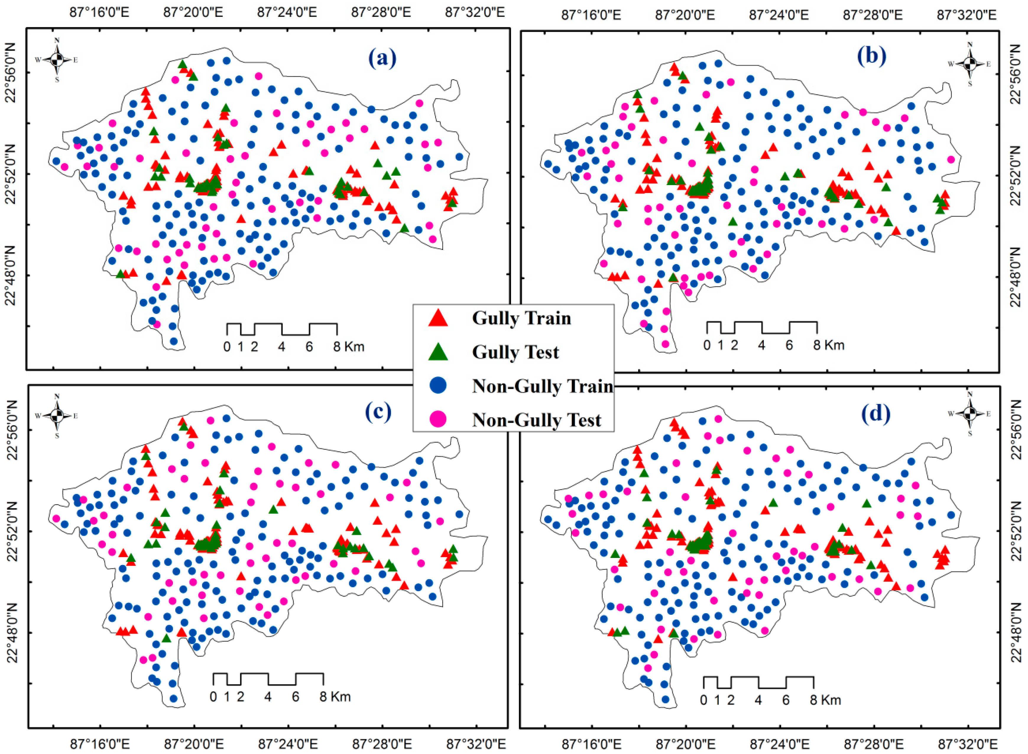
In machine learning, the ensemble model merges the final decision from multiple single models to develop the overall performance. The main advantage of the ensemble model is that it has the capability to improve the constancy and prediction accuracy of single MLA. Therefore, several ensemble models have been widely used for comprehensive analysis of hazard-related susceptibility mapping [21]. Previous research studies have shown that several ensemble approaches is used to get maximum accuracy in GES studies. Thus, in this research study we have also used a novel ensemble approach of BRT and Bagging model, as this newly developed ensemble approach has not been used in GES studies [15,28,50]. The ensemble of these two single MLAs i.e., BRT and bagging, was performed and analysed in freely available statistical programming language using ‘R’ software. The ensemble of BRT and bagging is more optimal in regards of GES assessment.

2.2.6. Resampling

Techniques of resampling are used to repeatedly drawing samples from a dataset and refitting a given configuration on each sample in order to understand more about the data configuration. Resampling approaches may be costly because they often allow similar statistical techniques to be applied to various subsets of the results. To acquire further knowledge about the configured model, resampling procedures refit a model of interest to samples generated from the training collection. We include details of the test-set estimation loss, for example, and the standard deviation and prejudice of our predictions for parameters. The test error is the mean error arising from utilizing a system of mathematical learning to forecast the answer of a new experiment, one that has not been used to practice the process. By comparison, the error in testing can be accurately determined by applying the process of predictive learning to the measurement used in its preparation. Various resampling algorithms are available including K-fold cross validation, cross validation (LOOCV), bootstrap and leave-one-out.

K-Fold Cross Validation

K-fold cross-validation is done by arbitrarily splitting the collection of results into K classes or folds of about the same scale. Related to leave-one-out cross validation, one of the K folds is used as the validation collection, while the other K-1 folds are used as the checking collection to produce the check error estimates for K. The predicted check error for K-fold cross validation arises from the sum of all results. In this study, we have chosen K-fold CV for splitting the dataset into training and validation purposes and the advantages of these resampling techniques are reduced bias through computational times being reduced, each data point has been tested exactly once for better performance and, finally, the variance of estimated result is reduced and increases the performance result.

Typical values for K are 4, 5 or 10 since they need fewer calculations than when K is equal to n. Cross-validation can be used both to determine how well a specific statistical learning process will do on recent data and to determine the lowest point in the calculated test mean square error curve, which can be helpful while contrasting statistical learning methods or whenever contrasting various degrees of versatility for a single statistical learning model.

2.2.7. Validation and Accuracy Assessment

Four statistical methods like responsiveness (TPR), specificity (TNR), positive predictive value (PPV) and negative predictive value (NPV) were used to test the performance of the machine-learning models used in the present research. The rationale behind the selection of the aforementioned validation techniques in this study is that the sensitivity of identifying the test of a correct measure of the true positive result was affected by problems, whereas the specificity test of correctly measuring the true negative result was not affected by problems. The positive and negative predictive values (PPV and NPV respectively) are the amounts of positive and negative outcomes, respectively, in data and experimental measures which are true positive and true negative findings. On the other hand, a common tool for verified the model’s output result is the ROC curve. The advantage of using the ROC curve in validation of the model’s performance is that ROC has been analysed through simple graphical representation and easily comparison between true and false positive relation. Alongside, ROC, AUC (area under the curve) is a non-parametric measurement, and therefore it is unaffected by abnormal distribution of variables. ROC is plotted on the x and y-axis, depending on the intensity and specificity. ROC’s AUC projects a model’s efficiency. The statistical principle and equation of that method are presented in depth in the previous studies [18]. Sensitivity (i.e., likelihood detection) raises the issue in the portion of the gully erosion observed is correctly labeled and its optimum value is 1. The precision (i.e., negative predictive meaning) raises the issue in the part of the non-gully erosion is accurately defined and its optimal meaning is 1 [42]. The AUC values of below 0.6, 0.6–0.7, 07–0.8, 0.8–0.9 and above 0.9 suggest that the model is poor, fair, average, outstanding and really high consistency, respectively. The ROC collection of training data generates the model’s performance rate, and tests the model’s suitability. ROC from the evaluation data collection indicates the model’s predictive importance and how strong or poor a predictive model is. Greater values of these predictive measures suggest the models’ higher performance [17]. The following equations have been used to calculate the aforementioned statistical analysis for validation.

$$TPR=\frac{TP}{\left(TP+FN\right)}$$

(14)

$$TNR=\frac{TN}{\left(TN+FP\right)}$$

(15)

$$PPV=\frac{Number of positive}{\left(Number of positive+Number of false positive\right)}$$

(16)

$$NPV=\frac{Number of true negatives}{\left(Number of true negatives+Number of false negative\right)}$$

(17)

$$AUC=\frac{\sum TP+\sum TN}{P+N}$$

(18)

3. Results

3.1. Multi-Collinearity Analysis

Multi-collinearity analysis is one of the widely used factor selection methods for evaluating the “non-independence” of gully erosion-inducing factors owing to strong correlations among variables, resulting in incorrect tests and unreliable predictions. Multi-collinearity is known in a dataset as a linear relationship between two or more gully-erosion conditioning variables [18,28]. The tolerance (TOL) and variance inflation factors (VIF) values are ≤ 0.1 and ≥ 10 respectively, which indicating good multi-collinearity among the variables in a dataset [17,51]. The multi-collinearity result (

Table 1. Multi-collinearity values for several gully erosion conditioning factors (GECFs).

Factors	Collinearity Statistics
	Fold 1		Fold 2		Fold 3		Fold 4
	TOL	VIF	TOL	VIF	TOL	VIF	TOL	VIF
SPI	0.231	4.330	0.233	4.288	0.236	4.237	0.251	3.981
Soil texture	0.225	4.450	0.268	3.736	0.255	3.924	0.854	1.171
Iron oxide	0.255	3.920	0.842	1.188	0.337	2.969	0.604	1.655
Lineament density	0.845	1.183	0.592	1.690	0.731	1.368	0.262	3.813
Geomorphology	0.716	1.397	0.749	1.335	0.458	2.183	0.728	1.374
Slope	0.321	3.113	0.339	2.953	0.819	1.221	0.380	2.630
Geology	0.244	4.104	0.950	1.053	0.251	3.982	0.310	3.228
Rainfall	0.278	3.599	0.779	1.283	0.271	3.692	0.328	3.051
Ferrous minerals	0.291	3.434	0.258	3.870	0.343	2.911	0.467	2.143
Profile curvature	0.602	1.662	0.515	1.942	0.575	1.738	0.695	1.439
Elevation	0.661	1.513	0.642	1.559	0.613	1.631	0.653	1.531
Plan curvature	0.428	2.339	0.374	2.675	0.412	2.425	0.482	2.074
Drainage density	0.412	2.425	0.421	2.376	0.376	2.658	0.378	2.644
NDVI	0.739	1.353	0.784	1.275	0.721	1.387	0.741	1.350
Distance to drainage	0.521	1.921	0.512	1.955	0.491	2.038	0.505	1.981
LULC	0.760	1.316	0.820	1.219	0.819	1.220	0.784	1.275
TWI	0.375	2.666	0.383	2.614	0.327	3.056	0.358	2.790
Aspect	0.477	2.097	0.776	1.288	0.321	3.113	0.225	4.447
Lithology	0.504	1.985	0.682	1.466	0.283	3.536	0.332	3.013
TRI	0.263	3.806	0.762	1.312	0.214	4.671	0.261	3.833

) shows that all variables are maintained threshold values of TOL and VIF for K4-fold training dataset i.e., Fold-1, Fold-2, Fold-3 and Fold-4, and are suitable for GES modelling and assessment.

3.2. Determine Best Parameters

The tune parameters of the BRT model suggest that the K-4 fold CV of the resampling algorithm has a higher interaction depth (3) than the other re-sampling methods (

Table 2. Tune parameters of boosted regression tree (BRT) model based on resampling algorithms.

Resampling	Number of Trees	Interaction Depth	Shrinkage	Number of Minobsin Node
1 fold CV	50	2	0.1	10
2 fold CV	50	2	0.1	10
3 fold CV	50	2	0.1	10
4 fold CV	150	3	0.1	10

), whereas the bagging tune parameters suggest that the K-4 fold CV of the resampling method has a maximum cost (64) with a sigma value of 0.0483 in comparison with the other resampling approaches (

Table 3. Tune parameters of bagging model based on resampling algorithms.

Resampling	Sigma	Cost
1 fold CV	0.0507	0.5
2 fold CV	0.0478	0.5
3 fold CV	0.0671	0.25
4 fold CV	0.0483	64

). In the case of BRT-bagging tune parameters, the m try value of the K-4 fold CV has the best output relative to the other resampling methods, which implies an equal number of trees (

Table 4. Tune parameters of BRT-bagging model based on resampling algorithms.

Resampling	Number of Tree	m Try
1 fold CV	200	8
2 fold CV	200	7
3 fold CV	200	8
4 fold CV	200	17

).

3.3. Relative Variables Importance of Gully Erosion Conditioning Factors (GECFs)

When evaluating susceptibility, it is crucial to choose the right modeling variables, as chosen factors largely depend on each other in the training dataset. Therefore, it is necessary to calculate the predictive capacity and multi-collinearity of the 20 chosen conditioning parameters while modeling GES. Therefore, the values for each conditioning parameter have been calculated by using the RF algorithm. The assessment of important variables of gully erosion was done through the mean decrease accuracy (MDA) index, using the RF model, as shown in

Table 5. Relative importance of gully causative factors

Factors	Relative Importance Value
	Fold 1	Fold 2	Fold 3	Fold 4
SPI	2.74	2.91	2.21	2.54
Soil Texture	23.47	24.51	25.34	24.84
Iron Oxide	0.75	0.78	0.81	0.64
Lineament Density	6.41	7.21	6.84	7.91
Geomorphology	48.75	47.21	50.28	52.48
Slope	72.41	76.85	74.61	75.51
Geology	15.24	16.28	17.21	16.24
Rainfall	10.28	12.54	13.08	11.45
Ferrous Minerals	27.54	24.58	27.14	25.41
Profile Curvature	54.27	55.44	52.47	53.47
Elevation	42.84	44.74	41.75	40.81
Plan Curvature	5.85	6.41	5.78	5.5
Drainage Density	65.74	65.86	64.79	66.71
NDVI	9.82	8.75	9.14	8.92
Distance To Drainage	4.65	5.52	4.21	5.71
LULC	68.41	65.82	66.78	70.21
TWI	30.28	32.28	31.42	34.72
Aspect	28.51	27.63	29.45	26.58
Lithology	27.68	27.45	26.94	27.12
TRI	14.56	14.92	15.71	15.52

. The findings suggest that the slope, drainage density, profile curvature, geomorphology and soil texture with their values of 76.85 (K2-Fold), 66.71 (K4-Fold), 55.44 (K2-Fold), 52.48 (K4-Fold) and 25.34 (K3-Fold) respectively, are of the greater importance in gully development and their formation, while the rest of the other variables, iron oxide, stream power index (SPI), distance to drainage and lineament density with their value of 0.64 (K4-Fold), 2.21 (K3-Fold), 4.21 (K3-Fold) and 6.41 (K1-Fold) respectively, are of less importance in the occurrence of gullies and their expansion. From the variables importance analysis, it was stated that the conditioning factors of slope, drainage density, profile curvature, soil texture are highly positively related with the formation of gullies and their development in this particular study area.

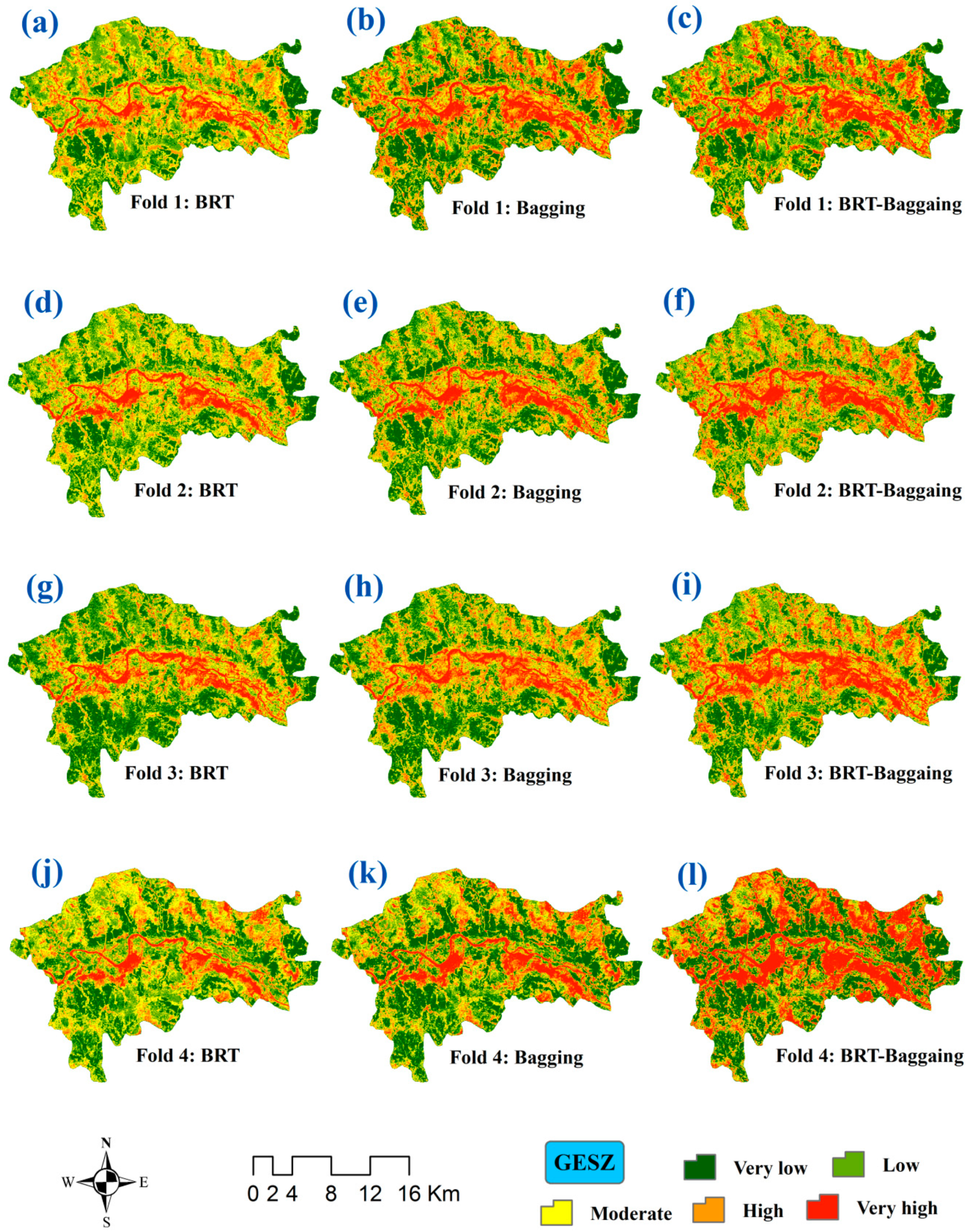
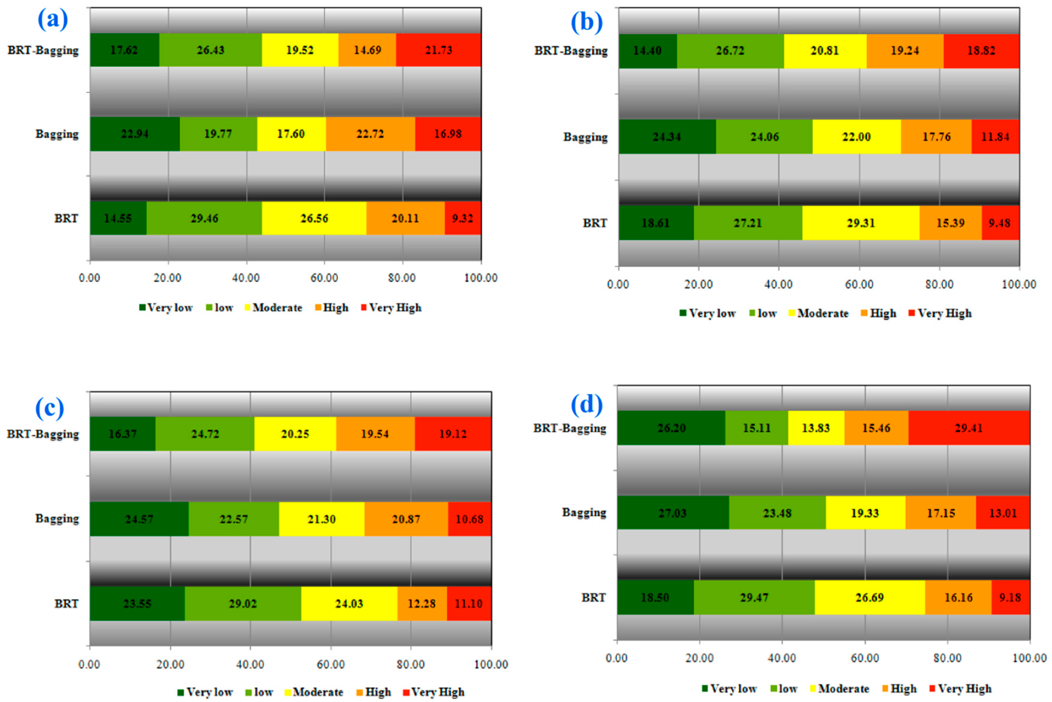
3.4. Modeling of Gully Erosion Susceptibility (GES) Mapping

It is essential to choose several appropriate parameters for modeling and evaluating natural hazards susceptibility assessment, as chosen factors in the training dataset depend on each other to produce uncertainty in the experiments. Moreover, when predicting GES, it is important to quantify the predictive efficiency and multi-collinearity of the 20 selected conditioning variables, so that the importance of variables is calculated in an accurate way. MLA such as BRT, bagging, BRT-bagging and four resampling approaches (Fold-1 CV, Fold-2 CV, Fold-3 CV and Fold-4) have been used to assess the position of gully erosion in the GES maps. The output of the ensemble machine learning models was determined by testing the efficiency of standalone machine-learning models (BRT, bagging) in order to obtain the precision the erosion susceptibility of Garhbeta-I C.D. Block (Figure 5). In the case of the BRT model, a GES map using the four fold CV (Figure 5a,d,g,j) have demonstrates the slight variation among the very high susceptibility zones (

Table 6. Distribution of GES classes

Susceptibility Class	BRT	Bagging	BRT-Bagging
Fold 1	(Value in %)
Very Low	14.55	22.94	17.62
Low	29.46	19.77	26.43
Moderate	26.56	17.60	19.52
High	20.11	22.72	14.69
Very High	9.32	16.98	21.73
Fold 2	(Value in %)
Very Low	18.61	24.34	14.40
Low	27.21	24.06	26.72
Moderate	29.31	22.00	20.81
High	15.39	17.76	19.24
Very High	9.48	11.84	18.82
Fold 3	(Value in %)
Very Low	23.55	24.57	16.37
Low	29.02	22.57	24.72
Moderate	24.03	21.30	20.25
High	12.28	20.87	19.54
Very High	11.10	10.68	19.12
Fold 4	(Value in %)
Very Low	18.50	27.03	26.20
Low	29.47	23.48	15.11
Moderate	26.69	19.33	13.83
High	16.16	17.15	15.46
Very High	9.18	13.01	29.41

) and these values were 9.32%, 9.48%, 11.10% and 9.18% for the fold-1, fold-2, fold-3 and fold-4 respectively. In the BRT model, the maximum percentage (23.55%) of very low susceptibility zone was found in fold-3 followed by fold-2 (18.61%), fold-4 (18.50%) and fold-1 (14.55%). The maximum gullies and their erosional activities were found along two sides of the river and some isolated patches throughout the study area.

In the case of the bagging approach, very high erosion zone is noticed in fold-1 (Figure 5b) with an aerial coverage of 16.98% followed by fold-4 (13.04%), fold-2 (11.84%) and fold-3 (10.68%), and their respective GES maps shown in Figure 5k,e,h. On the other side, very low susceptibility zones are found in fold-4 (27.03%) followed by fold-3 (24.57%), fold-2 (24.34%) and fold-1 (22.94%). In the ensemble of BRT-Bagging model, it is found that there is little bit variation in the very high susceptibility zones among the four folds i.e., fold-1: 21.73% (Figure 5c), fold-2: 18.82% (Figure 5f), fold-3: 19.12% (Figure 5i) and fold-4: 29.41% (Figure 5l) than the other two models used in GES mapping. In a similar way, maximum coverage of very low susceptibility zone is found in fold-4 (26.20%) followed by fold-1 (17.62%), fold-3 (16.37%) and fold-2 (14.40%). The graphical representation of four folds CV’s percentage area shows in Figure 6.

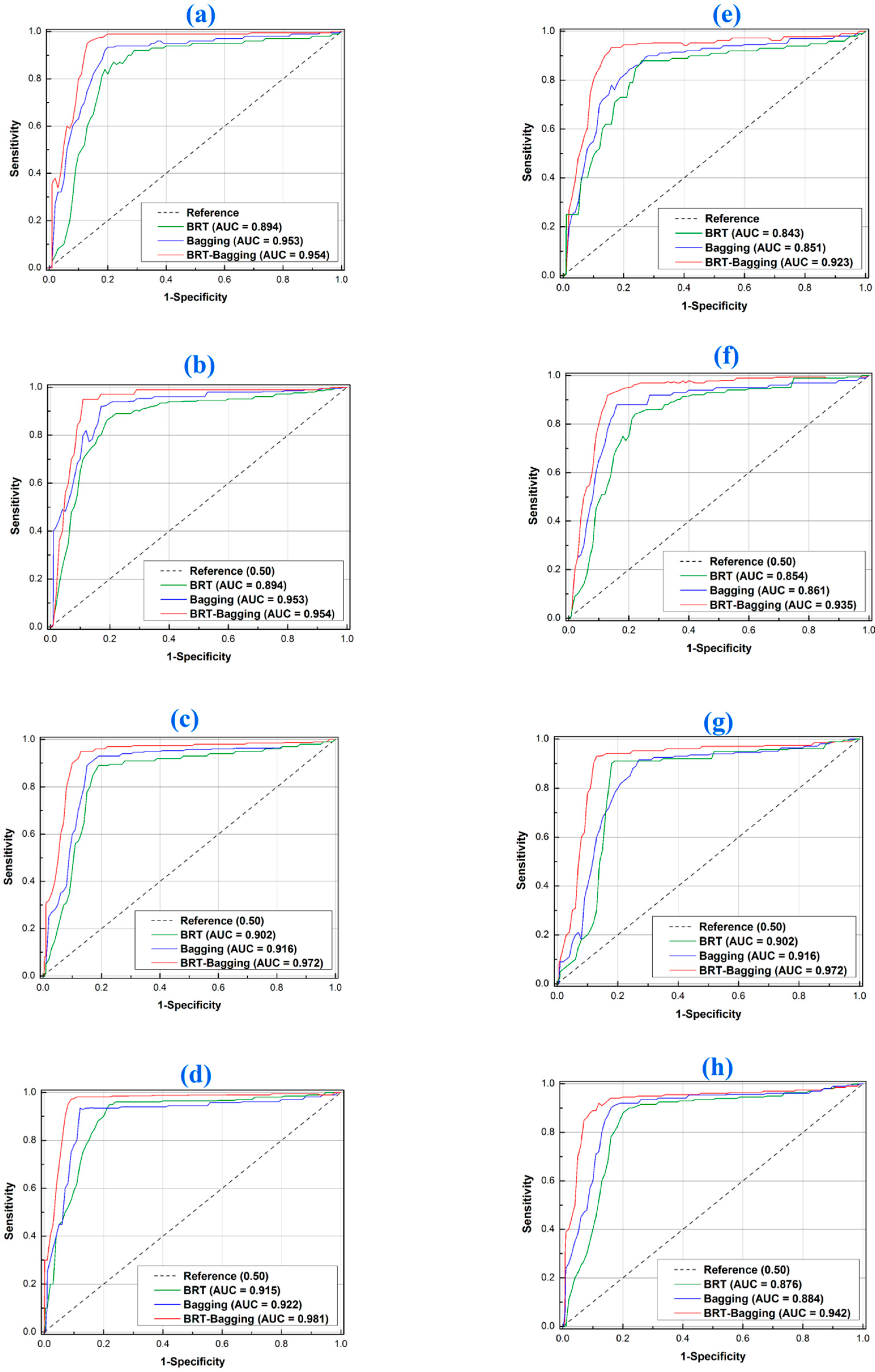
3.5. Validation of GES Models

The accuracy of all the maps obtained from four K-folds of BRT, bagging and BRT-bagging models were tested by the sensitivity, specificity, NPV, PPV and ROC curves analysis. The validation results show precisely that the K-4 fold BRT, K-4 fold bagging and K-4 fold BRT-bagging models with ROC values for the training dataset are 0.915, 0.922, 0.981 and for the tested dataset are 0.876, 0.884 and 0.942, respectively, and had an excellent level of accuracy (

Table 7. Predictive capability of head gully erosion models using train and test dataset.

Models	Resampling	Stage	Evaluate Parameters
			Sensitivity	Specificity	NPV	PPV	AUC
BRT	Fold 1	Train	0.84	0.87	0.84	0.86	0.874
		Test	0.79	0.83	0.77	0.84	0.843
	Fold 2	Train	0.89	0.9	0.92	0.93	0.894
		Test	0.83	0.75	0.74	0.77	0.854
	Fold 3	Train	0.86	0.82	0.81	0.89	0.902
		Test	0.81	0.75	0.71	0.75	0.863
	Fold 4	Train	0.85	0.87	0.88	0.83	0.915
		Test	0.83	0.84	0.77	0.8	0.876
Bagging	Fold 1	Train	0.89	0.92	0.9	0.89	0.937
		Test	0.74	0.74	0.71	0.81	0.851
	Fold 2	Train	0.85	0.91	0.89	0.87	0.953
		Test	0.82	0.69	0.71	0.76	0.861
	Fold 3	Train	0.92	0.89	0.91	0.88	0.916
		Test	0.72	0.82	0.67	0.84	0.856
	Fold 4	Train	0.86	0.89	0.82	0.91	0.922
		Test	0.79	0.85	0.75	0.71	0.884
BRT-Bagging	Fold 1	Train	0.94	0.92	0.96	0.93	0.967
		Test	0.91	0.89	0.91	0.89	0.923
	Fold 2	Train	0.91	0.94	0.91	0.95	0.954
		Test	0.83	0.85	0.89	0.91	0.935
	Fold 3	Train	0.94	0.93	0.96	0.93	0.972
		Test	0.76	0.86	0.86	0.9	0.938
	Fold 4	Train	0.94	0.96	0.91	0.92	0.981
		Test	0.83	0.87	0.8	0.9	0.942

). Among the three models used in this research analysis, BRT-bagging is the best fit model as its AUC value is 0.972 in K-3 fold and also high in sensitivity (0.94), specificity (0.93), NPV (0.96) and PPV (0.93) in the training dataset. The other two models i.e., bagging and BRT with their AUC value of 0.953 in K-2 fold and 0.915 in K-4 fold rank second and third respectively for GES assessment in this research study. The validation of graphical representation of ROC-AUC curve analysis maps for training and tested dataset is shown in Figure 7. Several previous gully erosion susceptibility (GES) studies have been carried out by using BRT and bagging models separately. In this study we have used a novel ensemble of the BRT-bagging approach and which is also shown that this ensemble approach is more robustness for GES assessment. Previous research work on GES assessment by using BRT model in the Bayazeh Watershed, Iran [30] and in the Valasht Watershed, Iran [32] have shows that AUC value in single BRT model is much lower i.e., 0.834 and 0.894 respectively than the ensemble of BRT-bagging. Another research work on GES evaluation by using the ensemble of complex proportional assessment of alternatives (COPRAS)-frequency ratio (FR)-BRT in the Najafabad watershed, Iran [31] has shows that AUC value is 0.972, which is also lower than the AUC value (0.981) of the BRT-bagging approach used in this study. Similarly, another research study on GES assessment in Rabat Turk watershed, Iran [33] based on the ensemble of bagging and reduced error pruning tree (REPtree) have shown AUC value is 0.871, which is also lower than the present ensemble approach of BRT-Bagging. Thus, in view of the result of accuracy assessment it is concluded that the proposal of novel ensemble approach of BRT-bagging is more accurate for gully erosion as well as any kind of natural hazards susceptibility assessment.

4. Discussion

Throughout this research, the scientific field-based approach was investigated through the application of ensemble machine-learning models of K-4 folds CV with BRT, bagging and BRT-bagging for the creation of gully development susceptibility maps, taking into consideration observed gully locations. Methods with resampling have been utilized for this research study, as resampling is a method that may support all of the analysis employed. While, unlike resampling, empirical sampling distributions do not solve all inferential problems, they will help to generate new statistics and bring robustness to other conventional ones [36]. Since modeling gully erosion sensitivity, it is important to quantify the predictive potential and multi-collinearity of the 20 chosen conditioning parameters, therefore the values of each conditioning variable have been determined [20,27]. In contrast, few experiments have mainly focused on gully erosion in order to establish and forecast a relation between gully and its absence, keeping in mind a number of variables incorporating within machine learning models used here [14,17,52]. Therefore, we have measured the importance value of every causal parameter behind the presence of gully locations in the study area of Garhbeta I C.D. Block. The results are correlated with the assumption that the frequency of gully erosion depends on the volume of the runoff area above the gully and in many other variables such as slope, elevation, drainage density, soil texture, percentage of clay, NDVI and land use.

Numerous ensemble models are applicable, but new and updated techniques and approaches for spatial modeling of GES are necessary. Therefore, three machine-learning algorithms namely BRT, Bagging and BRT-Bagging with four resampling approaches (K-1 fold CV, K-2 fold CV, K-3 fold CV and K-4 fold CV) were used to assess the efficiency of machine-learning models and to determine the precise GES maps and gully locations based on the determined 20 significant parameters. Modeling efficiency evaluation reveals that the ideal approach is a set of models K-4 BRT-bagging, K-4 bagging and K-4 BRT machine learning approaches with excellent precision of 0.981, 0.922 and 0.915, respectively, in the corresponding susceptibility categories of the gully positions relative to the majority of the ensemble machine learning methods. In fact, the ensemble of K-4 fold BRT, K-4 fold bagging and K-4 fold BRT-bagging improves the generalization of base predictors for gully positions. It is obvious from the field photos (Figure 1) that there are more gully development sites in and around the study region than others division of land use. Therefore, this phenomenon demonstrates that the effect of land use on gully development is very much effective. Unscientific management strategies and land use modification have been observed to play a crucial role in a regional scale of gully development, as subsurface piping and gully headcut experiences have led to the creation and development of gullies. Our results are comparable with those in which gully erosion is largely triggered by precipitation, land use, clay percentage and elevation [17,18,27]. In addition, the resampling-based ensemble machine-learning models (K-4 fold BRT, K-4 fold Bagging and K-4 fold BRT-Bagging) established that gully erosion sites are depend more accurately on a regional scale than the global perspective. Gully erosion is one of the most important causes of severe soil erosion in the study region and is a main source of sediment supply in the lower region. These negative consequences have caused considerable damage to the economy in the region. Therefore appropriate management measures should have to be introduced, taking into consideration of the local environment of the present study area.

5. Conclusions

Stronger knowledge of the conditioning factors impacting the frequency of gully erosion is important for the sustainability of areas prone to soil erosion. Throughout this study, the use of two single machine-learning algorithm i.e., BRT, bagging and an ensemble of BRT-bagging, as well as a four K-folds CV, rendered it possible to analyze the results of factors impacting the frequency of these gully erosion characteristics in the study area of Garhbeta I C. D. Block. A multi-collinearity study was used to identify 20 gully erosion susceptibility (GES) causal parameters and their function in gully development. In addition, the importance of these causal parameters was also evaluated, where seven variables, including slope, LULC, drainage density, profile curvature, geomorphology, ferrous minerals and soil texture, had the strongest impact on gully erosion in the study region. For modeling of gully erosion, 75% of the gully erosion sites were used for training and the remaining 25% for model validation. Validation of the models was made using the ROC-AUC curve and other statistical analyses. The results validation mainly demonstrated that the K-4 fold BRT, K-4 fold bagging and K-4 fold BRT-bagging models with ROC values of 0.981, 0.922 and 0.915, respectively, had an excellent accuracy level based on selected relevant parameters. The susceptibility map of gully erosion obtained in this study region can be used to manage land and water conversations, land use planning and, eventually, sustainable development throughout the region.

References

1. Gayen, A.; Pourghasemi, H.R. 30—Spatial modeling of gully erosion: A new ensemble of CART and GLM data-mining algorithms. In Spatial Modeling in GIS and R for Earth and Environmental Sciences; Pourghasemi, H.R., Gokceoglu, C., Eds.; Elsevier: Amsterdam, The Netherlands, 2019; pp. 653–669. ISBN 978-0-12-815226-3. [Google Scholar]
2. Poesen, J.; Govers, G. Gully erosion in the loam belt of Belgium: Typology and control measures. In Soil Erosion on Agricultural Land Proceedings of A Workshop Sponsored by the British Geomorphological Research Group, Coventry, UK, 1989; John Wiley & Sons Ltd.: Hoboken, NJ, USA, 1990; pp. 513–530. [Google Scholar]
3. Poesen, J.W. Contribution of gully erosion to sediment production on cultivated lands and rangelands. In Proceedings of an International Symposium, Exeter, UK, 15–19 July 1996 No. 236; IAHS: Wallingford, UK, 1996. [Google Scholar]
4. Poesen, J.; Vanwalleghem, T.; Deckers, J. Gullies and closed depressions in the loess belt: Scars of human–environment interactions. In Landscapes and Landforms of Belgium and Luxembourg; World Geomorphological Landscapes; Demoulin, A., Ed.; Springer International Publishing: Cham, Switzerland, 2018; pp. 253–267. ISBN 978-3-319-58239-9. [Google Scholar]
5. Poesen, J.; Nachtergaele, J.; Verstraeten, G.; Valentin, C. Gully erosion and environmental change: Importance and research needs. CATENA 2003, 50, 91–133. [Google Scholar] [CrossRef]
6. Das, B.; Pal, S.C.; Malik, S. Assessment of flood hazard in a riverine tract between Damodar and Dwarkeswar River, Hugli District, West Bengal, India. Spat. Inf. Res. 2018, 26, 91–101. [Google Scholar] [CrossRef]
7. Das, B.; Pal, S.C.; Malik, S.; Chakrabortty, R. Living with floods through geospatial approach: A case study of Arambag C.D. Block of Hugli District, West Bengal, India. SN Appl. Sci. 2019, 1, 329. [Google Scholar] [CrossRef] [Green Version]
8. Chowdhuri, I.; Pal, S.C.; Chakrabortty, R. Flood susceptibility mapping by ensemble evidential belief function and binomial logistic regression model on river basin of eastern India. Adv. Space Res. 2020, 65, 1466–1489. [Google Scholar] [CrossRef]
9. Malik, S.; Pal, S.C. Application of 2D numerical simulation for rating curve development and inundation area mapping: A case study of monsoon dominated Dwarkeswar river. Int. J. River Basin Manag. 2020, 1–11. [Google Scholar] [CrossRef]
10. Pal, S.; Shit, M. Application of RUSLE model for soil loss estimation of Jaipanda watershed, West Bengal. Spat. Inf. Res. 2017. [Google Scholar] [CrossRef]
11. Pal, S.C.; Chakrabortty, R. Modeling of water induced surface soil erosion and the potential risk zone prediction in a sub-tropical watershed of Eastern India. Model Earth Syst. Environ. 2019, 5, 369–393. [Google Scholar] [CrossRef]
12. Pal, S.C.; Chakrabortty, R. Simulating the impact of climate change on soil erosion in sub-tropical monsoon dominated watershed based on RUSLE, SCS runoff and MIROC5 climatic model. Adv. Space Res. 2019, 64, 352–377. [Google Scholar] [CrossRef]
13. Saha, A.; Ghosh, M.; Pal, S.C. Understanding the morphology and development of a rill-gully: An Empirical study of Khoai Badland, West Bengal, India. In Gully Erosion Studies from India and Surrounding Regions; Advances in Science, Technology & Innovation; Shit, P.K., Pourghasemi, H.R., Bhunia, G.S., Eds.; Springer International Publishing: Cham, Switzerland, 2020; pp. 147–161. ISBN 978-3-030-23243-6. [Google Scholar]
14. Al-Abadi, A.M.; Al-Ali, A.K. Susceptibility mapping of gully erosion using GIS-based statistical bivariate models: A case study from Ali Al-Gharbi District, Maysan Governorate, southern Iraq. Environ. Earth Sci. 2018, 77, 249. [Google Scholar] [CrossRef]
15. Chakrabortty, R.; Pal, S.C.; Chowdhuri, I.; Malik, S.; Das, B. Assessing the Importance of static and dynamic causative factors on erosion potentiality using SWAT, EBF with uncertainty and plausibility, logistic regression and novel ensemble model in a sub-tropical environment. J. Indian Soc. Remote Sens. 2020, 48, 765–789. [Google Scholar] [CrossRef]
16. Rahmati, O.; Haghizadeh, A.; Pourghasemi, H.R.; Noormohamadi, F. Gully erosion susceptibility mapping: The role of GIS-based bivariate statistical models and their comparison. Nat. Hazards 2016, 82, 1231–1258. [Google Scholar] [CrossRef]
17. Amiri, M.; Pourghasemi, H.R.; Ghanbarian, G.A.; Afzali, S.F. Assessment of the importance of gully erosion effective factors using Boruta algorithm and its spatial modeling and mapping using three machine learning algorithms. Geoderma 2019, 340, 55–69. [Google Scholar] [CrossRef]
18. Pourghasemi, H.R.; Yousefi, S.; Kornejady, A.; Cerdà, A. Performance assessment of individual and ensemble data-mining techniques for gully erosion modeling. Sci. Total Environ. 2017, 609, 764–775. [Google Scholar] [CrossRef] [Green Version]
19. Gayen, A.; Pourghasemi, H.R.; Saha, S.; Keesstra, S.; Bai, S. Gully erosion susceptibility assessment and management of hazard-prone areas in India using different machine learning algorithms. Sci. Total Environ. 2019, 668, 124–138. [Google Scholar] [CrossRef]
20. Rahmati, O.; Tahmasebipour, N.; Haghizadeh, A.; Pourghasemi, H.R.; Feizizadeh, B. Evaluating the influence of geo-environmental factors on gully erosion in a semi-arid region of Iran: An integrated framework. Sci. Total Environ. 2017, 579, 913–927. [Google Scholar] [CrossRef]
21. Azareh, A.; Rahmati, O.; Rafiei-Sardooi, E.; Sankey, J.B.; Lee, S.; Shahabi, H.; Ahmad, B.B. Modelling gully-erosion susceptibility in a semi-arid region, Iran: Investigation of applicability of certainty factor and maximum entropy models. Sci. Total Environ. 2019, 655, 684–696. [Google Scholar] [CrossRef]
22. Arabameri, A.; Asadi Nalivan, O.; Chandra Pal, S.; Chakrabortty, R.; Saha, A.; Lee, S.; Pradhan, B.; Tien Bui, D. Novel machine learning approaches for modelling the gully erosion susceptibility. Remote Sens. 2020, 12, 2833. [Google Scholar] [CrossRef]
23. Band, S.S.; Janizadeh, S.; Chandra Pal, S.; Saha, A.; Chakrabortty, R.; Shokri, M.; Mosavi, A. Novel ensemble approach of Deep Learning Neural Network (DLNN) model and Particle Swarm Optimization (PSO) algorithm for prediction of gully erosion susceptibility. Sensors 2020, 20, 5609. [Google Scholar] [CrossRef]
24. Puente, C.; Olague, G.; Smith, S.V.; Bullock, S.H.; Hinojosa-Corona, A.; González-Botello, M.A. A Genetic programming approach to estimate vegetation cover in the context of soil erosion assessment. Photogramm. Eng. Remote Sens. 2011, 77, 363–376. [Google Scholar] [CrossRef] [Green Version]
25. Puente, C.; Olague, G.; Trabucchi, M.; Arjona-Villicaña, P.D.; Soubervielle-Montalvo, C. Synthesis of vegetation indices using genetic programming for soil erosion estimation. Remote Sens. 2019, 11, 156. [Google Scholar] [CrossRef] [Green Version]
26. Cabral, A.I.R.; Silva, S.; Silva, P.C.; Vanneschi, L.; Vasconcelos, M.J. Burned area estimations derived from Landsat ETM+ and OLI data: Comparing genetic/ programming with maximum likelihood and classification and regression trees. ISPRS J. Photogramm. Remote Sens. 2018, 142, 94–105. [Google Scholar] [CrossRef]
27. Kariminejad, N.; Hosseinalizadeh, M.; Pourghasemi, H.R.; Bernatek-Jakiel, A.; Alinejad, M. GIS-based susceptibility assessment of the occurrence of gully headcuts and pipe collapses in a semi-arid environment: Golestan Province, NE Iran. Land Degrad. Dev. 2019, 30, 2211–2225. [Google Scholar] [CrossRef]
28. Roy, P.; Chakrabortty, R.; Chowdhuri, I.; Malik, S.; Das, B.; Pal, S.C. Development of different machine learning ensemble classifier for gully erosion susceptibility in gandheswari watershed of West Bengal, India. In Machine Learning for Intelligent Decision Science; Algorithms for Intelligent Systems; Rout, J.K., Rout, M., Das, H., Eds.; Springer: Singapore, 2020; pp. 1–26. ISBN 9789811536892. [Google Scholar]
29. Zhang, W.; Du, Z.; Zhang, D.; Yu, S.; Hao, Y. Boosted regression tree model-based assessment of the impacts of meteorological drivers of hand, foot and mouth disease in Guangdong, China. Sci. Total Environ. 2016, 553, 366–371. [Google Scholar] [CrossRef]
30. Arabameri, A.; Pradhan, B.; Lombardo, L. Comparative assessment using boosted regression trees, binary logistic regression, frequency ratio and numerical risk factor for gully erosion susceptibility modelling. CATENA 2019, 183, 104223. [Google Scholar] [CrossRef]
31. Arabameri, A.; Yamani, M.; Pradhan, B.; Melesse, A.; Shirani, K.; Tien Bui, D. Novel ensembles of COPRAS multi-criteria decision-making with logistic regression, boosted regression tree, and random forest for spatial prediction of gully erosion susceptibility. Sci. Total Environ. 2019, 688, 903–916. [Google Scholar] [CrossRef]
32. Zabihi, M.; Pourghasemi, H.R.; Motevalli, A.; Zakeri, M.A. Gully erosion modeling using GIS-based data mining techniques in Northern Iran: A comparison between boosted regression tree and multivariate adaptive regression spline. In Natural Hazards GIS-Based Spatial Modeling Using Data Mining Techniques; Advances in Natural and Technological Hazards Research; Pourghasemi, H.R., Rossi, M., Eds.; Springer International Publishing: Cham, Switzerland, 2019; pp. 1–26. ISBN 978-3-319-73383-8. [Google Scholar]
33. Nhu, V.-H.; Janizadeh, S.; Avand, M.; Chen, W.; Farzin, M.; Omidvar, E.; Shirzadi, A.; Shahabi, H.; Clague, J.J.; Jaafari, A.; et al. GIS-based gully erosion susceptibility mapping: A comparison of computational ensemble data mining models. Appl. Sci. 2020, 10, 2039. [Google Scholar] [CrossRef] [Green Version]
34. Shit, P.K.; Paira, R.; Bhunia, G.; Maiti, R. Modeling of potential gully erosion hazard using geo-spatial technology at Garbheta block, West Bengal in India. Model Earth Syst. Environ. 2015, 1, 2. [Google Scholar] [CrossRef]
35. Shit, P.K.; Maiti, R.K. Mechanism of gully-head retreat—A study at Ganganir Danga, Paschim Medinipur, West Bengal. Ethiop. J. Environ. Stud. Manag. 2012, 5, 332–342. [Google Scholar] [CrossRef] [Green Version]
36. Chernick, M.R. Resampling methods. WIREs Data Min. Knowl. Discov. 2012, 2, 255–262. [Google Scholar] [CrossRef]
37. Arabameri, A.; Pradhan, B.; Pourghasemi, H.R.; Rezaei, K.; Kerle, N. Spatial modelling of gully erosion using GIS and R programing: A comparison among three data mining algorithms. Appl. Sci. 2018, 8, 1369. [Google Scholar] [CrossRef] [Green Version]
38. Conforti, M.; Aucelli, P.P.C.; Robustelli, G.; Scarciglia, F. Geomorphology and GIS analysis for mapping gully erosion susceptibility in the Turbolo stream catchment (Northern Calabria, Italy). Nat. Hazards 2011, 56, 881–898. [Google Scholar] [CrossRef]
39. Barnes, N.; Luffman, I.; Nandi, A. Gully erosion and freeze-thaw processes in clay-rich soils, Northeast Tennessee, USA. GeoResJ 2016, 9–12, 67–76. [Google Scholar] [CrossRef]
40. Ollobarren, P.; Capra, A.; Gelsomino, A.; La Spada, C. Effects of ephemeral gully erosion on soil degradation in a cultivated area in Sicily (Italy). CATENA 2016, 145, 334–345. [Google Scholar] [CrossRef]
41. Arabameri, A.; Chen, W.; Loche, M.; Zhao, X.; Li, Y.; Lombardo, L.; Cerda, A.; Pradhan, B.; Bui, D.T. Comparison of machine learning models for gully erosion susceptibility mapping. Geosci. Front. 2020, 11, 1609–1620. [Google Scholar] [CrossRef]
42. Chen, W.; Shahabi, H.; Zhang, S.; Khosravi, K.; Shirzadi, A.; Chapi, K.; Pham, B.T.; Zhang, T.; Zhang, L.; Chai, H.; et al. Landslide susceptibility modeling based on GIS and novel bagging-based kernel logistic regression. Appl. Sci. 2018, 8, 2540. [Google Scholar] [CrossRef] [Green Version]
43. Breiman, L. Random forests. Mach. Learn. 2001, 45, 5–32. [Google Scholar] [CrossRef] [Green Version]
44. Hong, H.; Xiaoling, G.; Hua, Y. Variable selection using mean decrease accuracy and mean decrease gini based on random forest. In Proceedings of the 7th IEEE International Conference on Software Engineering and Service Science (ICSESS), Beijing, China, 26–28 August 2016; pp. 219–224. [Google Scholar]
45. Elith, J.; Leathwick, J.R.; Hastie, T. A working guide to boosted regression trees. J. Anim. Ecol. 2008, 77, 802–813. [Google Scholar] [CrossRef]
46. Elith, J.; Leathwick, J. Boosted Regression Trees for Ecological Modeling. Online Tutorial. 3 July 2011, p. 22. Available online: http://cran.r-project.org/web/packages/dismo/vignettes/brt.pdf (accessed on 1 November 2020).
47. Friedman, J.H. Greedy function approximation: A gradient boosting machine. Ann. Stat. 2001, 29, 1189–1232. [Google Scholar] [CrossRef]
48. Breiman, L. Bagging predictors. Mach. Learn. 1996, 24, 123–140. [Google Scholar] [CrossRef] [Green Version]
49. Hong, H.; Liu, J.; Bui, D.T.; Pradhan, B.; Acharya, T.D.; Pham, B.T.; Zhu, A.-X.; Chen, W.; Ahmad, B.B. Landslide susceptibility mapping using J48 Decision Tree with AdaBoost, Bagging and Rotation Forest ensembles in the Guangchang area (China). CATENA 2018, 163, 399–413. [Google Scholar] [CrossRef]
50. Chakrabortty, R.; Pal, S.C.; Sahana, M.; Mondal, A.; Dou, J.; Pham, B.T.; Yunus, A.P. Soil erosion potential hotspot zone identification using machine learning and statistical approaches in eastern India. Nat. Hazards 2020. [Google Scholar] [CrossRef]
51. Hair, J.F. Multivariate Data Analysis; Pearson Prentice Hall: Upper Saddle River, NJ, USA, 2006; ISBN 978-0-13-032929-5. [Google Scholar]
52. Bernatek-Jakiel, A.; Poesen, J. Subsurface erosion by soil piping: Significance and research needs. Earth Sci. Rev. 2018, 185, 1107–1128. [Google Scholar] [CrossRef]
Figure 1. Location of study area.
Remotesensing 12 03675 g001
Figure 2. Methodological flowchart for the present research work.
Remotesensing 12 03675 g002
Figure 3. Training and validation dataset of gully and non-gully head-cuts (a) Fold-1; (b) Fold-2; (c) Fold-3; (d) Fold-4.
Remotesensing 12 03675 g003
Figure 4. Causative factors of gully erosion; (a) Slope, (b) Aspect, (c) Elevation, (d) Profile Curvature, (e) Plan Curvature, (f) Topographic wetness index (TWI), (g) Stream power index (SPI), (h) Terrain Ruggedness Index (TRI), (i) Rainfall, (j) Drainage density, (k) Distance to Drainage, (l) Geomorphology, (m) land use land cover (LULC), (n) Normalized Vegetation Difference Index (NDVI), (o) Ferrous minerals, (p) Iron oxide, (q) Soil texture, (r) Geology, (s) Lineament density, (t) Lithology.
Remotesensing 12 03675 g004aRemotesensing 12 03675 g004bRemotesensing 12 03675 g004cRemotesensing 12 03675 g004d
Figure 5. Gully erosion susceptibility (GES) maps prepared by using Fold-1 (a) BRT, (b) Bagging, (c) BRT-Bagging; Fold-2 (d) BRT, (e) Bagging, (f) BRT-Bagging; Fold-3 (g) BRT, (h) Bagging, (i) BRT-Bagging and Fold-4 (j) BRT, (k) Bagging, (l) BRT-Bagging.
Remotesensing 12 03675 g005
Figure 6. Graphical percentage distributions of each GES class generated by using the GES models of (a) Fold-1, (b) Fold-2, (c) Fold-3 and (d) Fold-4.
Remotesensing 12 03675 g006
Figure 7. Validation of results using area under the curve of the receiver operating characteristic: using training datasets of (a) Fold-1, (b) Fold-2, (c) Fold-3 and (d) Fold-4; and using testing datasets of (e) Fold-1, (f) Fold-2, (g) Fold-3 and (h) Fold-4.
Remotesensing 12 03675 g007