Technical Note

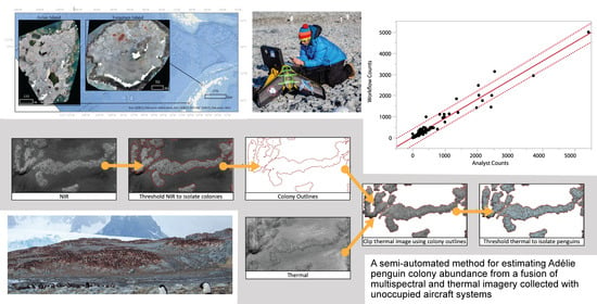
A Semi-Automated Method for Estimating Adélie Penguin Colony Abundance from a Fusion of Multispectral and Thermal Imagery Collected with Unoccupied Aircraft Systems

1
Geospatial Ecology of Marine Megafauna Lab, Marine Mammal Institute, Department of Fisheries and Wildlife, Hatfield Marine Science Center, Oregon State University, Newport, OR 97365, USA
2
Environment, Ecology, and Energy Program, University of North Carolina at Chapel Hill, Chapel Hill, NC 27599, USA
3
Division of Marine Science and Conservation, Nicholas School of the Environment, Duke University Marine Laboratory, Beaufort, NC 28516, USA
*
Author to whom correspondence should be addressed.
Remote Sens. 2020, 12(22), 3692; https://0-doi-org.brum.beds.ac.uk/10.3390/rs12223692
Submission received: 23 October 2020 / Revised: 6 November 2020 / Accepted: 9 November 2020 / Published: 11 November 2020
(This article belongs to the Special Issue She Maps)

Abstract

:
Monitoring Adélie penguin (Pygoscelis adeliae) populations on the Western Antarctic Peninsula (WAP) provides information about the health of the species and the WAP marine ecosystem itself. In January 2017, surveys of Adélie penguin colonies at Avian Island and Torgersen Island off the WAP were conducted via unoccupied aircraft systems (UAS) collecting optical Red Green Blue (RGB), thermal, and multispectral imagery. A semi-automated workflow to count individual penguins using a fusion of multispectral and thermal imagery was developed and combined into an ArcGIS workflow. This workflow isolates colonies using multispectral imagery and detects and counts individuals by thermal signatures. Two analysts conducted manual counts from synoptic RGB UAS imagery. The automated system deviated from analyst counts by −3.96% on Avian Island and by 17.83% on Torgersen Island. However, colony-by-colony comparisons revealed that the greatest deviations occurred at larger colonies. Matched pairs analysis revealed no significant differences between automated and manual counts at both locations (p > 0.31) and linear regressions of colony sizes from both methods revealed significant positive relationships approaching unity (p < 0.0002. R2 = 0.91). These results indicate that combining UAS surveys with sensor fusion techniques and semi-automated workflows provide efficient and accurate methods for monitoring seabird colonies in remote environments.

Graphical Abstract

1. Introduction

For wildlife biologists, occupied aircraft surveys are crucial tools that inform both ecological studies and conservation decisions by providing critical information on the status and trajectories of vertebrate animal populations, including assessments of colonial seabirds [1,2]. Unfortunately, occupied aircraft surveys can be expensive, logistically challenging and, depending on the organisms and habitat, they can be risky. Indeed, one study found that aviation-based accidents were the leading cause of work related mortality for wildlife biologists [3]. These factors may be especially important in remote locations that exhibit harsh conditions.
Some of the harshest environments in which humans conduct wildlife surveys are found in polar regions, including the Western Antarctic Peninsula (WAP). The WAP is remote and largely accessible only in the austral summer, making population assessments for most vertebrate species, including key species of interest such as the Adélie penguin (Pygoscelis adeliae), extremely challenging. In most locations, aerial support for penguin population surveys is severely limited, or completely lacking due to large costs and logistical constraints. A significant amount of effort is dedicated to monitoring Adélie penguin colonies in the WAP as they are believed to be sensitive indicators of ecological change [4]. In some portions of the northern WAP, Adélie penguins have been decreasing since the 1970s [5] and given the rapidly changing climate in this region, it is especially important to track colony trajectories. Accurate assessments of Adélie breeding colonies are especially important—by counting both adults and juveniles, biologists can monitor the trajectory of colonies and assess how breeding success may relate to environmental stressors [5].
To conduct surveys of Adélie penguins on the Western Antarctic Peninsula, scientists typically access colonies on foot, walking across challenging terrain in cold temperatures for extended periods of time to count thousands of penguins by hand [6]. Another, faster, survey method uses portable GPS systems to measure the perimeter of each colony, defined as areas covered in guano, and uses these areas to estimate abundance using general or site-specific ratios of penguins or nests per square meter of guano [7,8]. Surveys from aerial or satellite imagery are a compelling alternative to ground-based counts (where possible) as they are more efficient, and, given the challenges associated with oblique ground-based assessments, often more accurate [9].
Several studies have used aerial imagery to estimate penguin colony sizes. An early study showed that using kites to take pictures of breeding colonies along the Western Antarctic Peninsula could be a more cost-efficient method to count Adélie penguin populations, especially for large colonies [5]. More recently, studies have used helicopter-based aerial surveys [10] and UAS surveys [11,12] to manually detect and count penguins from imagery in ArcGIS. It is possible to improve both the efficiency and accuracy of wildlife population counts by using automated counting tools [13,14] and studies using automation to count bird populations started in the late 1980s [15,16]. Since then, there have been an array of studies testing and validating automated processes for detecting, counting, and mapping bird populations [14,17,18,19,20,21,22].
Studies focused on penguins have used both satellite and aerial imagery from occupied aircraft and UAS. Several studies have developed methods using high-resolution satellite imagery using a variety of techniques including supervised classification [23], geographic-based object analysis [24], and maximum likelihood multivariate classification [8]. Others have developed methods for aerial imagery using methods such as semi-automated thresholding [25], and image segmentation [4].
Most of these studies focused on detecting and quantifying the area of penguin colonies by separating out the guano in the color images [8,23,24,25]. Trathan (2004) [4] manually isolated colonies and then applied a threshold to isolate individual penguins from the images. Building on this, McNeill et al. (2011) [25] applied a threshold twice, first to isolate the colony and then a second time to isolate individual penguins. This workflow was released as an interactive GUI (Geographical User Interface) for the MatLab software computational environment that allowed the user to edit the results by adding or deleting penguins that were missed or falsely identified.
Unoccupied aircraft systems (UAS) are increasingly used to augment or replace occupied aircraft surveys [26] and have been used in a large variety of both terrestrial and marine studies; examples include assessing tropical forest recovery [27], facilitating precision agriculture [28], measuring coastal topology [29,30] and quantifying fluctuating geomorphology [31,32], sampling surface temperature of oceans [33] and streams [34], conducting blue whale photogrammetry [35], and estimating right whale body condition [36]. UAS can provide a more efficient method for conducting wildlife surveys [37,38,39,40] as they cover relatively large areas in single flights that take considerably less time than surveys on foot. Additionally, UAS can carry a variety of sensors (either simultaneously or on sequential flights), providing opportunities to enhance and automate methods of population estimation through sensor fusion approaches that combine optical Red Green Blue (RGB), thermal infrared (IR) and multispectral (e.g., near-infrared and red-edge) reflectance data for detecting objects of interest.
The value of using thermal IR imagery for wildlife population surveys has been demonstrated for a variety of bird and mammal species, largely because they tend to emit heat, making them distinguishable from their habitats. This includes studies of a variety of bird [41,42,43,44] and mammal species [45,46,47,48,49]. The use of multispectral imagery in aerial surveys for animals is less widely applied, but some applications show promise for detecting marine species [50]. Furthermore, multispectral imagery can clearly be used to define habitat parameters that help focus or constrain other remote sensing methods to detect and enumerate organisms in visible or thermal imagery [51].
The present study establishes a semi-automated workflow to estimate Adélie penguin colony sizes through the fusion of multispectral and thermal imagery collected with a fixed wing UAS. This workflow initially uses multispectral reflectance of guano in near infrared (NIR) wavelengths to identify colony areas that are then assessed via thermal imagery to detect and count birds. This workflow was converted into a series of open source parameterized ArcGIS tools sensu McNeill et al. (2011) [25]. This multispectral/thermal assessment workflow compared favorably with manual counts generated by UAS-generated RGB imagery of the same colonies on the same day, demonstrating that integrating thermal and multispectral imagery from UAS surveys can improve the efficiency and accuracy of Adélie penguin population surveys.

2. Methods

2.1. Study Sites

This study was conducted on two islands on the WAP: Approximately 1/3 of Avian Island (67°46′21″S, 68°53′19″W) and all of Torgersen Island (approximately 64°46′17″S, 64° 04′31″W), shown in Figure 1. The surveys were conducted in late January and early February of 2017 during the Adélie penguin breeding season.

2.2. Data Collection

All UAS data were collected using the classic senseFly eBee, a commercially available fixed wing UAS. The eBee has a light-weight foam airframe powered by a single rear-mounted brushless electric motor powered by a lithium polymer battery. It has a wing-span of 96 cm and weighs 0.7 kg. During surveys, the eBee UAS followed a pre-programmed three-dimensional flight path guided by a precision GPS sensor, a high-resolution barometer, ground-sensing camera and wind-speed indicators as in Arona et al. (2018) [52]. Speed over ground varied between 11 and 14 m per second and failsafe logic was set to return the UAS to the landing zone if it experienced anomalies in sensor performance or extreme wind conditions (greater than 12 m per second), and it telemetered flight data to the operator in real time. The instrument was launched by hand and recovered after a linear approach/landing at a predetermined 10 m radius region. RGB imagery was collected with a 12.1 megapixel Canon S110 camera. Thermal imagery was collected using the senseFly Thermomap sensor, a self-calibrating 640 × 512-pixel thermal infrared camera with a marketed precision of 0.1 °C (senseFly LLC) and accuracy of approximately 1 °C [49]. Multispectral imagery was collected using the Parrot Sequoia sensor, a 1 megapixel camera sensitive to green (530–570 nm), red (640–680 nm), red edge (730–740 nm) and near infrared (770–810 nm) wavelengths. All UAS flights were preprogrammed using the eMotion software package (senseFly, Switzerland) and flight durations ranged between 15 and 22 min at an altitude of approximately 85 m above ground level. Take-off and linear landings for all flights were conducted at least 50 m away from colonies being assessed to reduce potential disturbance. Flight plans were designed to capture imagery on sequential short lines, to reduce artifacts that arise when applying Structure from Motion (SfM) techniques to images with long time intervals between acquisition times. In both study locations, all flights were conducted between 11:00 a.m. and 3:00 p.m. local time (GMT-5). Penguin colony flights were conducted sequentially (RGB, Multispectral, and thermal IR) with <20 min between flights. Weather at both locations was similar, with air temperatures between 3 and 6 °C, partly cloudy skies, and visibility greater that 15 km. The final ground sampling distance (GSD) of all images used in the analysis are available in Table 1.

2.3. Data Processing

All UAS imagery from all three sensors was analyzed with the SfM Pix4D Mapper software (Pix4D SA, Prilly, Switzerland) to create products used in subsequent analyses. For the multispectral data collected from the Sequoia, only the four multispectral channels were considered, and the RGB imagery was disregarded due to it being low quality in comparison to dedicated RGB sampling. The processing followed the typical multispectral processing Pix4D pipeline under a direct georeferencing scenario [53] that included image alignment, tie point extraction, bundle block adjustment (BBA), the generation of point clouds, digital surface modeling (DSM), and the creation of orthomosaic and reflectance maps used in subsequent analyses. This pipeline used one set of radiometric calibration target images per flight to generate calibrated reflectance values. Thermomapper imagery was also processed using the standard Pix4D pipeline, similar to Seymour et al. (2017) [49]. The RGB orthomosaics were also edited in Pix4D to correct for errors caused by misaligned tiles and obvious animals moving between images.
The multispectral, thermal and RGB layers were not aligned, so they were georectified with easily identifiable features in all layers using the Georeferencing tool in ArcGIS Desktop 10.5.1 [54] prior to any analysis. The georeferenced images were exported for analysis using bilinear interpolation as the image cells contained continuous data.

2.4. Penguin Count Data

The RGB orthomosaics were tiled and imported into the iTAG software package [55] where penguin adults and chicks within colonies were counted in each tile by two trained analysts. Chicks were distinguished from adults by their grey plumage. Counts were then separated by individual colonies in ArcGIS. In this study, we use the term colony to refer to individual enclosed areas of guano containing nests.

2.5. Population Count Workflow

Automated population counts and colony density estimates were calculated using a sequential combination of thermal and multispectral imagery. The general workflow (Supplementary Material Figure S1), isolates penguin colonies as polygons by applying a threshold to multispectral imagery, and then extracts colony areas from the georectified thermal imagery by overlaying these multispectral colony polygons. The number of penguins within each colony was counted using the thermal imagery, and the density of penguins per colony was calculated by dividing the number of penguins per colony by its area. We chose different multispectral approaches for each island based on greatest contrast between guano and the background, demonstrating how both single-band reflectance, or reflectance indices can be employed in this workflow. For Avian Island, single-band near infrared (NIR) reflectance was used to isolate the outlines of colonies, whereas the Normalized Difference Vegetation Index (NDVI) (NIR − red band/NIR + red band, [56]) was used to outline colonies on Torgersen Island. Operationally, the workflow was divided into three separate stages in order to create a toolset that applied easily to other imagery sets and allow the user to enter site-specific parameters at different stages. Details on these stages and the workflow toolbox are detailed below.

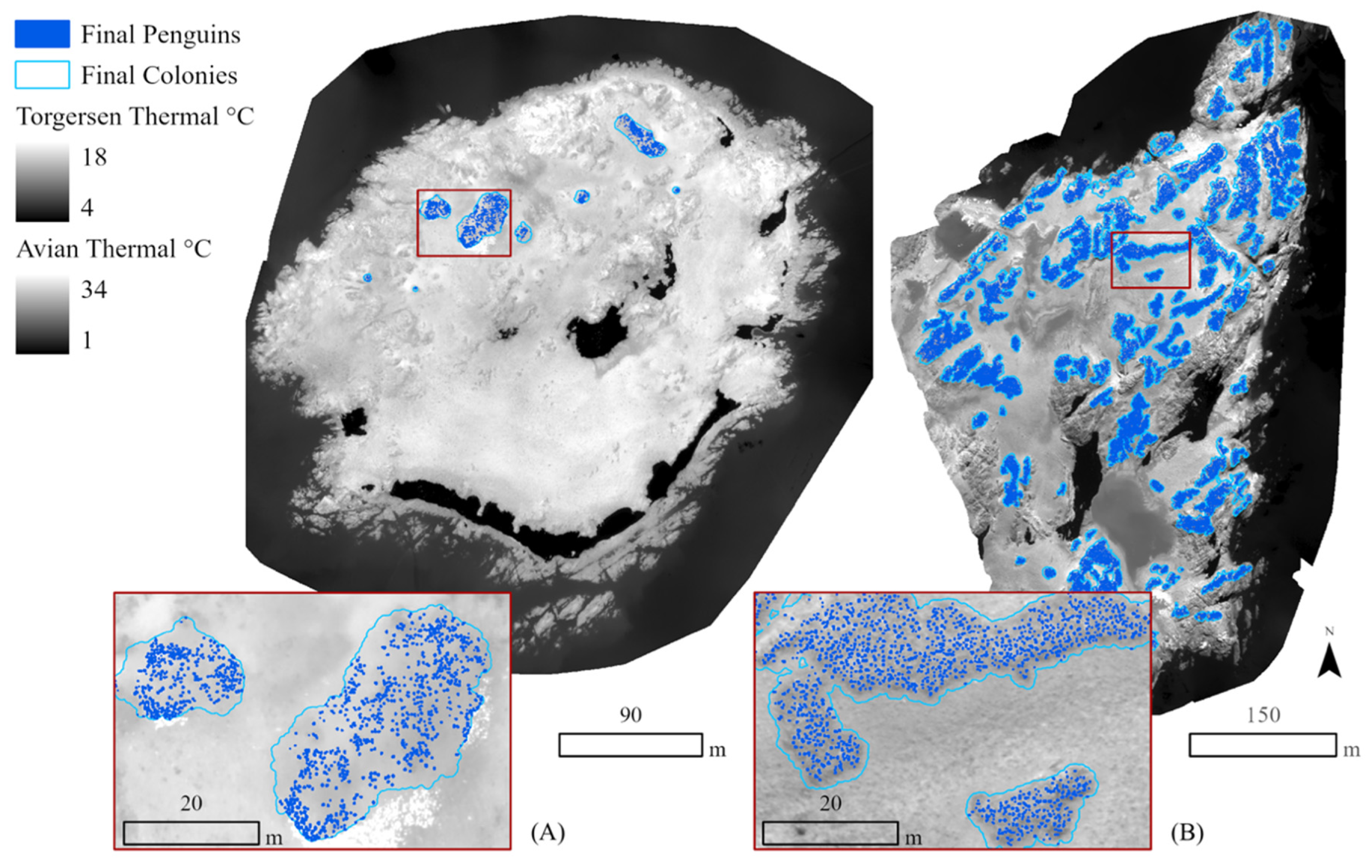
2.5.1. Step 1. Multispectral Colony Delineation

To identify individual penguin colonies, we examined NIR or NDVI reflectance values of known guano patches throughout the image to define a threshold value that captured the lower limit of guano reflectance values. To determine the threshold, we sampled approximately 20 points throughout the colonies, selecting guano pixels representing a range of reflectance values. Each point identified the value of one pixel. The thresholds selected were 0.42 and 0.16 for Avian and Torgersen Island, respectively. We then selected all pixels within each orthomosaic with values above the threshold and converted them to polygons. Polygons greater than 0.3 m2 were selected and then dissolved to create continuous colony polygons to eliminate holes created by the less reflective penguins. An area threshold value of 0.3 m2 was chosen during development through observations that polygons below this value tended to be non-guano pixels. Finally, we added 0.6 m buffers to each polygon and then dissolved them to create the complete suite of colony polygons. A buffer size of 0.6 m was chosen because we found that this distance covered gaps in colonies caused by penguin clumps without joining neighboring colonies.

2.5.2. Steps 2 and 3. Thermal Colony Assessment

Multispectral colonies were then assessed for features on the islands that might have similar reflectance values to guano, such as dirty snow, ice, or vegetation, which were removed. A small number of colonies were outlined manually because the extent of the NIR imagery did not overlap completely with the thermal imagery, with a section of the island not included in the NIR imagery. We then combined the selected colonies with the drawn colonies and added 0.5 m buffers to the complete colony polygons to create a final comprehensive colony mask. This final buffer was applied to avoid losing area when clipping out the high values created by the high pass filter, described below, along the outline of each colony.
The final buffered colony mask was used to extract penguin colony areas from the thermal imagery to limit the scope of further analysis, Figure 2 shows this step of the process. This approach focuses assessments to within colonies, reducing the likelihood that further steps would be biased by including warm regions of the ground and by counting other birds in the area such as giant petrels or sheathbills. While there was no way to distinguish between penguins and sheathbills within a colony from the thermal imagery, the number of sheathbills was minimal.
As penguins appear warmer than their background in thermal imagery, they could be identified and enumerated within our thermal colony regions. However, they were not all uniform in temperature; on Avian Island, the range of thermal values was from 1.33 to 34.11 and on Torgersen Island the range was from 3.77 to 17.68. Moreover, in some cases their proximity to each other posed problems for detecting individuals. As in Seymour et al. (2017) [49], we applied a high pass filter to thermal IR data to help isolate individual penguins within extracted colonies by enhancing their edges.
Through comparisons with RGB data, a threshold value was established for the presence of a penguin. We resampled the high pass filter output to a cell size of 0.08 m2, to spatially capture the thermal signature of a penguin. Next, we selected all cell values above the threshold for a penguin signal and then used the unbuffered colony mask to remove the colony outlines and extract thermal signals of penguins from the colony areas. The high pass threshold values were 4.5 and 0.3 for Avian and Torgersen Island, respectively. We then converted these signals into penguin polygons to create the final individual penguin layer. Finally, we spatially joined the penguin and colony layers in order to calculate density. In some cases, penguins were so close together that they had merged into one larger thermal hotspot that was not deconstructed through high pass filtering. In these cases, we used the average area of a penguin identified above to calculate how many penguins were within one hotspot. On both islands, penguins at least 0.3 m apart were distinguished as separate individuals, and about one third of the thermal signals were clumps larger than the size of one penguin. Finally, we calculated the density of penguins per colony by dividing the number of penguins in a colony by that colony’s area. The final colony and penguin layers are show in Figure 3. The ArcGIS toolbox and code for this project are available at https://github.com/cbirdferrer/penguin-counting. Data and code are available at https://0-doi-org.brum.beds.ac.uk/10.7924/r4cv4jq6j.

2.6. Comparison with Manual Imagery Counts

We compared total and per colony penguin abundance generated by the automated workflow with the average analyst count for each colony. To do this, points created in iTAG were imported into ArcGIS and then joined with the colony shapes to calculate colony abundance and density. We also estimated per colony abundance using a common ratio for breeding colonies in the region (two penguins per square meter of guano) [7] and used analyst counts and guano areas to calculate the ratio at the study sites to compare the accuracy of the workflow against the analyst counts.
Initial distribution plots of the densities of penguins per colony on each island were created and a matched pairs analysis was used to examine the relationship between automated and manual counts across colony sizes. Bivariate linear regressions of the automated counts vs. analyst counts were conducted to assess how well the automated counts predicted manual counts on each island. These assessments were all conducted using JMP (JMP Pro, Version 14.0.0. SAS Institute Inc., Cary, NC, USA, 1989–2019).

3. Results

3.1. Manual and Automated Counts

The average analyst count was 49,483 at the Avian Island study site and 1189 on Torgersen Island (Table 2). The automated count was 47,525 at the Avian Island study site and 1401 on Torgersen Island (Figure 3). Table 3 summarizes the results from each method used to estimate the population at the Avian Island study site. Using the average analyst count as the expected, this resulted in a percent error of 3.96% on Avian Island and 17.83% on Torgersen Island.

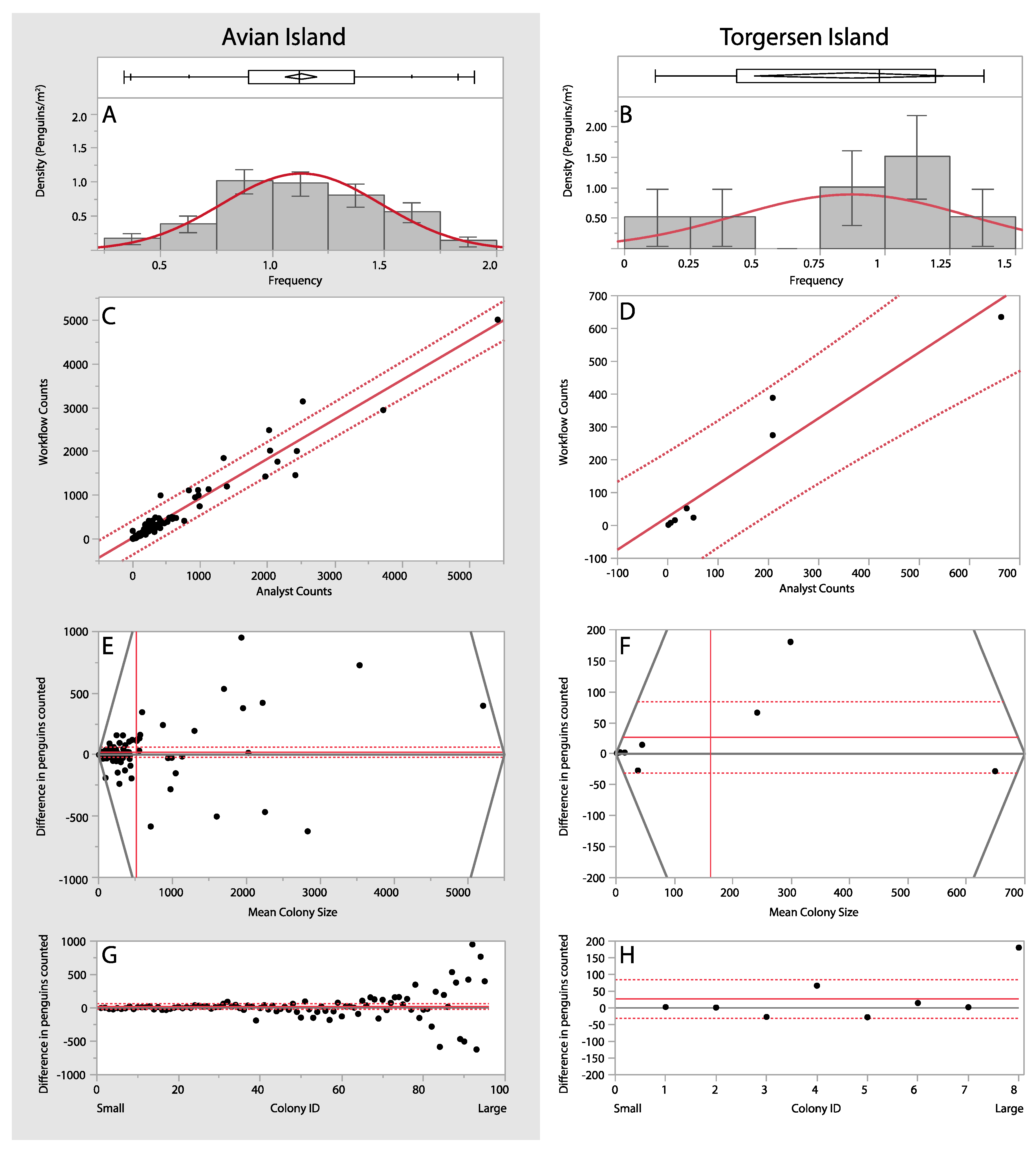
3.2. Area-Based Assessments

The total area of guano, as calculated by the workflow, was 38,318.75 m2 at the Avian Island study site and 1439.3 m2 on Torgersen Island (Figure 3). Therefore, application of the two penguins per square meter ratio indicates that there would be 76,637 penguins at the Avian Island study site and 2879 penguins on Torgersen Island. Using the average of the workflow and analyst counts and the area of guano from the workflow, we estimated a ratio of 1.27 penguins per square meter at the Avian Island study site and 0.90 penguins per square meter on Torgersen Island. When we used these ratios to estimate the population, we estimated that there were 48,665 penguins at the Avian Island study site and 1295 penguins on Torgersen Island during the time of the surveys (Table 3).

3.3. Manual vs. Automated Counts

As shown in Figure 4A,B, the distribution of colony densities was approximately normal for both Avian (W = 0.99, p = 0.74) and Torgersen Island (W = 0.87, p = 0.15). The results of the regression indicate a strong positive relationship between the analyst average counts and the workflow counts on Avian Island (Figure 4C: R2 = 0.94, F(1,93) = 1466.68, p(>F) < 0.0001, beta = 0.90, p(>|t|) < 0.0001). Figure 4C shows that very few colonies deviate from expected and those colonies that fell outside of the confidence interval were larger colonies. Similarly, the results of the regression on Torgersen Island revealed a strong positive relationship between the analyst average counts and the workflow counts (Figure 4D: R2 = 0.91, F(1,6) = 64.37, p(>F) < 0.0002, beta = 1.00, p(>|t|) < 0.0002). Figure 4D shows that all colonies fell within the confidence interval and that larger colonies deviated most from the line. A matched pairs t-test was used to compare the average analyst counts and workflow counts (Figure 4E,F). At the Avian Island study site there was no significant difference between the average analyst count (M = 49,482.5, SD = 2803.678) and the workflow count (47,525); t(94) = 0.96, p = 0.34. There was also no significant difference found between the average analyst count (M = 1189, SD = 8.49) and the workflow count (1401) on Torgersen Island; t(7) = −1.09, p = 0.31. Figure 4G,H show that the difference between the analyst average count and the workflow count increases with colony size.

4. Discussion

The results of the present study demonstrate an efficient and repeatable approach that fuses high-resolution multispectral and thermal data to assess Adélie penguin colonies on the WAP. Furthermore, our study illustrates how these data can be employed to rapidly generate colony abundance data through an easy-to-use, semi-automated GIS workflow.
The matched pairs and regression analyses revealed no significant differences between model and analyst counts, and regressions indicate that the average of analyst counts has a strong relationship to workflow counts. However, the percent errors differed considerably between the two islands. The automated workflow calculated 1958 fewer penguins at the Avian Island study site than the average analyst count yet estimated 212 more penguins on Torgersen Island than the average analyst count. There are several factors that may have contributed to the accuracy of both the analyst counts and the workflow, including artifacts in the RGB and thermal imagery that could not be controlled for.
First, at the time of the flight, the sun angle created shadows that looked like penguins. Consequently, when penguins were tightly clustered it became difficult to distinguish a penguin from the shadow of another. Additionally, light-colored juveniles were sometimes within the shadow of an adult, meaning that shadows could easily be mistaken for a juvenile or vice versa. In some cases, the size and color of the juveniles also made it difficult to differentiate them from rocks on the edges of the colonies. The matched pairs analysis (Figure 4) revealed that the difference between the automated and manual counts increased with colony size, suggesting that analyst accuracy decreased with colony size, and, therefore, mirroring the conclusions of Fraser et al. (1999) [5], this workflow may be especially useful for larger colonies.
The percent error on Torgersen may have been higher than the percent error at the Avian Island study site due to the presence of several patches of hot pixels along the edges of the colonies in the thermal imagery that were not penguins. Because of their location, some of these patches were included in the colony polygons and therefore likely contributed to the workflow count being greater than the average analyst count. These hot spots may have been rocks heated by the sun; so, to minimize the chance of this happening in the future, flights should be conducted earlier in the day or on an overcast day.
Similar to McNeill et al. (2011) [25] and LaRue et al. (2014) [23], we have demonstrated the use of guano signatures to isolate colonies in high-resolution remote sensing imagery and estimate penguin abundance. While previous studies have done this using RGB imagery, we used the reflectance of guano in NIR imagery. Guano reflects strongly in the NIR component of the electromagnetic spectrum because it remains high in nutrients and pigments associated with the krill-based Adélie penguin diet [57]. NIR is typically used for analyzing the nutrient content of soil, but it has also been used to analyze the nutrient content of food. One study found that NIR is especially good for nutrient analysis of homogenous crushed food [58]. Interestingly, in the present study guano had a more distinct contrast from the background in NIR imagery at the Avian Island study site in contrast to NDVI imagery on Torgersen Island. We propose two potential explanations for this difference in reflectance. One possible explanation is that the guano was clearly drier on Avian Island, an observation made by observers in the field during UAS flights. This difference in wetness could have caused a difference in the spectral reflectance pattern of the guano [59]. Another possibility is that the diet of the penguins on Avian Island contained less krill, leading to less red pigment in the guano [59]. A study focused on using UAS to study variability in guano spectral reflectance throughout the breeding season, under different moisture conditions, is needed to fully understand this difference.
LaRue et al. (2014) [23] developed a supervised classification method to quantify the guano area and estimate Adélie penguin abundance in satellite-based remote sensing imagery. A central component of the classification was a distinction between old and new guano color signals. However, the observed difference in guano multispectral signals in the present study indicates that the within-year guano signal can be variable across locations and may be dependent on local precipitation patterns, something that has not been addressed in previous studies. Understanding how this signal may change within years and across years is important for studies looking to use multispectral signals to detect penguin colonies from remotely sensed imagery. Applying UAS in such a study would be beneficial as they collect higher-resolution data and their immediacy would allow for more frequent studies, including on cloudy days that limit satellite-based remote sensing approaches. The high-resolution imagery also allows for detailed population counts, as opposed to area-based density estimates.
That being said, employing the guano area as part of the present workflow provides for the calculation of site-specific and colony-specific ratios of penguins per square meter of guano. Intriguingly, the ratios were different for each island and they differed from previously published ratios. The ratio is clearly influenced by reproductive seasonality [10], which might account for the differences between the study sites. This could also be explained by the different conditions of the islands and the behavior of birds at those colonies; Torgersen is farther north and has warmed more than Avian Island in recent years, and the Adélie penguin colonies on Torgersen have significantly decreased [6]. UAS surveys at both locations were conducted at different times across more than 3 degrees of latitude and approximately 400 km of straight-line distance, perhaps capturing phenological differences in colony attendance by penguins. Furthermore, deviations in colony trajectories at both locations may explain why the penguin-to-area ratio would be different across colonies at these sites. Finally, if this ratio is an indicator for population health—where a high density indicates a healthy colony [6]—these may reflect deviations in overall penguin colony health at these two sites.

5. Conclusions

The combination of UAS imagery and the fusion of multispectral imagery provides significant opportunities to create robust and efficient workflows for populations of penguins, and likely other colonial seabirds. The tools generated in the present study can be parameterized for each study location and species and are therefore applicable to a variety of cases. The established workflow was divided into three tools applied sequentially, as some of the input parameters depend on intermediate products of the overall workflow. While this reduces efficiency to some extent, the overall workflow still requires less time than ground surveys or manual counts, and the added control over the inputs increases accuracy and provides flexibility for applying this approach to other species or other habitats. Furthermore, this fundamental geoprocessing approach is likely to be more accessible and adaptable than other fully automated approaches such as CNNs for some researchers. Where a CNN-based approach would require significant amounts of training data, greater computation power, and machine learning training, the present approach only requires ArcGIS and training in geospatial analysis.
This approach can also be adapted to a variety of contexts rapidly; using a fusion of imagery could be useful for enumerating other species that congregate in areas with varying reflectance spectra. Additionally, using an automated approach helps eliminate potential errors associated with variability between individual analysts’ counts, and provides for greater methodological consistency and comparability of survey data over time. Furthermore, the number of light and low-cost thermal and dual RGB/Thermal cameras is quickly growing, meaning that the efficacy of approaches like this will improve. Future work should focus on developing automated methods for distinguishing between adult and juvenile penguins in order to estimate breeding pairs, an important metric used in penguin population surveys. The results of the present study demonstrate how modern high-resolution remote sensing methods can be used to advance the efficiency and safety of Adélie penguin population surveys in rapidly changing habitats of the Western Antarctic Peninsula.

Supplementary Materials

The following are available online at https://0-www-mdpi-com.brum.beds.ac.uk/2072-4292/12/22/3692/s1, Figure S1: Workflow of the population count ArcGIS workflow.

Author Contributions

Conceptualization, C.N.B., J.D., D.W.J.; methodology, C.N.B., J.D., D.W.J.; software, C.N.B.; investigation and formal analysis, C.N.B., A.H.D., D.W.J.; resources, D.W.J.; data curation, C.N.B., A.H.D.; writing—original draft preparation, C.N.B.; writing—review and editing, D.W.J., A.H.D.; visualization, C.N.B., D.W.J.; supervision, D.W.J.; project administration, C.N.B., D.W.J., J.D.; funding acquisition, C.N.B., D.W.J. All authors have read and agreed to the published version of the manuscript.

Funding

This research was funded by the National Science Foundation (NSF Prime Award # PLR-1440435 to Oregon State University through Subaward #7 (GG008855); the Duke portion of that grant was via Oregon State University Subaward U0975A-A, LTER Palmer, Antarctica) and the World Wildlife Fund (WWF Grant # 283-2124).

Acknowledgments

We would like to acknowledge the support of the Palmer Station LTER Program, the Duke University Marine Robotics and Remote Sensing Lab and the Oregon State University Geospatial Ecology of Marine Megafauna Lab. We would like to thank John Fay for providing feedback on the development of the user inputs for the toolset. Data were collected under ACA Permit No. 2017-034.

Conflicts of Interest

The authors declare no conflict of interest.

References

  1. Agnew, D.J. Review—The CCAMLR Ecosystem Monitoring Programme. Antarct. Sci. 1997, 9. [Google Scholar] [CrossRef]
  2. Lancia, R.A.; Kendall, W.L.; Pollock, K.H.; Nichols, J.D. Estimating the number of animals in wildlife populations. In Techniques for Wildlife Investigations and Management; Braun, C.E., Ed.; Wildlife Society: Bethesda, MD, USA, 2005; pp. 106–153. [Google Scholar]
  3. Sasse, D.B. Job-Related Mortality of Wildlife Workers in the United States, 1937–2000. Wildl. Soc. Bull. 2003, 31, 1015–1020. [Google Scholar]
  4. Trathan, P.N. Image analysis of color aerial photography to estimate penguin population size. Wildl. Soc. Bull. 2004, 32, 332–343. [Google Scholar] [CrossRef]
  5. Fraser, W.R.; Carlson, J.C.; Duley, P.A.; Holm, E.J.; Patterson, D.L. Using Kite-Based Aerial Photography for Conducting Adélie Penguin Censuses in Antarctica. Waterbirds Int. J. Waterbird Biol. 1999, 22, 435. [Google Scholar] [CrossRef]
  6. Montaigne, F. Fraser’s Penguins: A Journey to the Future in Antarctica, 1st ed.; Henry Holt and Co.: New York, NY, USA, 2010; ISBN 978-0-8050-7942-5. [Google Scholar]
  7. Stonehouse, B. Introdcution: The Spheniscidae. In The Biology of Penguins; The Macmillan Press: London, UK, 1975; pp. 1–15. [Google Scholar]
  8. Waluda, C.M.; Dunn, M.J.; Curtis, M.L.; Fretwell, P.T. Assessing penguin colony size and distribution using digital mapping and satellite remote sensing. Polar Biol. 2014, 37, 1849–1855. [Google Scholar] [CrossRef]
  9. Hollings, T.; Burgman, M.; van Andel, M.; Gilbert, M.; Robinson, T.; Robinson, A. How do you find the green sheep? A critical review of the use of remotely sensed imagery to detect and count animals. Methods Ecol. Evol. 2018, 9, 881–892. [Google Scholar] [CrossRef]
  10. Southwell, C.; McKinlay, J.; Low, M.; Wilson, D.; Newbery, K.; Lieser, J.L.; Emmerson, L. New methods and technologies for regional-scale abundance estimation of land-breeding marine animals: Application to Adélie penguin populations in East Antarctica. Polar Biol. 2013, 36, 843–856. [Google Scholar] [CrossRef]
  11. Pfeifer, C.; Barbosa, A.; Mustafa, O.; Peter, H.U.; Rümmler, M.C.; Brenning, A. Using fixed-wing uav for detecting and mapping the distribution and abundance of penguins on the South Shetlands Islands, Antarctica. Drones 2019, 3, 39. [Google Scholar] [CrossRef] [Green Version]
  12. Mustafa, O.; Braun, C.; Esefeld, J.; Knetsch, S.; Maercker, J.; Pfeifer, C.; Rümmler, M.C. Detecting Antarctic Seals And Flying Seabirds by UAV. ISPRS Ann. Photogramm. Remote Sens. Spat. Inf. Sci. 2019, 4, 141–148. [Google Scholar] [CrossRef] [Green Version]
  13. Laliberte, A.S.; Ripple, W.J. Automated Wildlife Counts from Remotely Sensed Imagery. Wildl. Soc. Bull. 2003, 31, 362–371. [Google Scholar]
  14. Hodgson, J.C.; Mott, R.; Baylis, S.M.; Pham, T.T.; Wotherspoon, S.; Kilpatrick, A.D.; Raja Segaran, R.; Reid, I.; Terauds, A.; Koh, L.P. Drones count wildlife more accurately and precisely than humans. Methods Ecol. Evol. 2018, 9, 1160–1167. [Google Scholar] [CrossRef] [Green Version]
  15. Bajzak, D.; Piatt, J.F. Computer-Aided Procedure for Counting Waterfowl on Aerial Photographs. Wildl. Soc. Bull. 1990, 18, 125–129. [Google Scholar]
  16. Gilmer, D.S.; Brass, J.A.; Strong, L.L.; Card, D.H. Goose Counts from Aerial Photographs Using an Optical Digitizer. Wildl. Soc. Bull. 1988, 16, 204–206. [Google Scholar]
  17. Chabot, D.; Francis, C.M. Computer-automated bird detection and counts in high-resolution aerial images: A review. J. Field Ornithol. 2016, 87, 343–359. [Google Scholar] [CrossRef]
  18. Cunningham, D.J.; Anderson, W.H.; Anthony, R.M. An image-processing program for automated counting. Wildl. Soc. Bull. 1996, 24, 345–346. [Google Scholar]
  19. Groom, G.; Stjernholm, M.; Nielsen, R.D.; Fleetwood, A.; Petersen, I.K. Remote sensing image data and automated analysis to describe marine bird distributions and abundances. Ecol. Inform. 2013, 14, 2–8. [Google Scholar] [CrossRef]
  20. Sardà-Palomera, F.; Bota, G.; Viñolo, C.; Pallarés, O.; Sazatornil, V.; Brotons, L.; Gomáriz, S.; Sardà, F. Fine-scale bird monitoring from light unmanned aircraft systems. IBIS (Lond. 1859) 2012, 154, 177–183. [Google Scholar] [CrossRef]
  21. Andrew, M.E.; Shephard, J.M. Semi-automated detection of eagle nests: An application of very high-resolution image data and advanced image analyses to wildlife surveys. Remote Sens. Ecol. Conserv. 2017, 3, 66–80. [Google Scholar] [CrossRef] [Green Version]
  22. Lyons, M.B.; Brandis, K.J.; Murray, N.J.; Wilshire, J.H.; McCann, J.A.; Kingsford, R.T.; Callaghan, C.T. Monitoring large and complex wildlife aggregations with drones. Methods Ecol. Evol. 2019, 10, 1024–1035. [Google Scholar] [CrossRef] [Green Version]
  23. LaRue, M.A.; Lynch, H.J.; Lyver, P.O.B.; Barton, K.; Ainley, D.G.; Pollard, A.; Fraser, W.R.; Ballard, G. A method for estimating colony sizes of Adélie penguins using remote sensing imagery. Polar Biol. 2014, 37, 507–517. [Google Scholar] [CrossRef]
  24. Witharana, C.; Lynch, H.J. An object-based image analysis approach for detecting penguin guano in very high spatial resolution satellite images. Remote Sens. 2016, 8, 375. [Google Scholar] [CrossRef] [Green Version]
  25. McNeill, S.; Barton, K.; Lyver, P.; Pairman, D. Semi-automated penguin counting from digital aerial photographs. In Proceedings of the 2011 IEEE International Geoscience and Remote Sensing Symposium, Vancouver, BC, Canada, 24–29 July 2011; IEEE: Piscataway, NJ, USA, 2011; pp. 4312–4315. [Google Scholar]
  26. Johnston, D.W. Unoccupied Aircraft Systems in Marine Science and Conservation. Ann. Rev. Mar. Sci. 2019, 11, 439–463. [Google Scholar] [CrossRef] [PubMed] [Green Version]
  27. Zahawi, R.A.; Dandois, J.P.; Holl, K.D.; Nadwodny, D.; Reid, J.L.; Ellis, E.C. Using lightweight unmanned aerial vehicles to monitor tropical forest recovery. Biol. Conserv. 2015, 186, 287–295. [Google Scholar] [CrossRef] [Green Version]
  28. Zhang, C.; Kovacs, J.M. The application of small unmanned aerial systems for precision agriculture: A review. Precis. Agric. 2012, 13, 693–712. [Google Scholar] [CrossRef]
  29. Mancini, F.; Dubbini, M.; Gattelli, M.; Stecchi, F.; Fabbri, S.; Gabbianelli, G.; Mancini, F.; Dubbini, M.; Gattelli, M.; Stecchi, F.; et al. Using Unmanned Aerial Vehicles (UAV) for High-Resolution Reconstruction of Topography: The Structure from Motion Approach on Coastal Environments. Remote Sens. 2013, 5, 6880–6898. [Google Scholar] [CrossRef] [Green Version]
  30. Seymour, A.C.; Ridge, J.T.; Rodriguez, A.B.; Newton, E.; Dale, J.; Johnston, D.W. Deploying Fixed Wing Unoccupied Aerial Systems (UAS) for Coastal Morphology Assessment and Management. J. Coast. Res. 2018, 34, 704–717. [Google Scholar] [CrossRef]
  31. Papakonstantinou, A.; Topouzelis, K.; Pavlogeorgatos, G.; Papakonstantinou, A.; Topouzelis, K.; Pavlogeorgatos, G. Coastline Zones Identification and 3D Coastal Mapping Using UAV Spatial Data. ISPRS Int. J. Geo-Inf. 2016, 5, 75. [Google Scholar] [CrossRef] [Green Version]
  32. Seymour, A.C.; Ridge, J.T.; Newton, E.; Rodriguez, A.B.; Johnston, D.W. Geomorphic response of inlet barrier islands to storms. Geomorphology 2019, 339, 127–140. [Google Scholar] [CrossRef]
  33. Inoue, J.; Curry, J.A. Application of Aerosondes to high-resolution observations of sea surface temperature over Barrow Canyon. Geophys. Res. Lett. 2004, 31, L14312. [Google Scholar] [CrossRef] [Green Version]
  34. Jensen, A.M.; Neilson, B.T.; McKee, M.; Chen, Y. Thermal remote sensing with an autonomous unmanned aerial remote sensing platform for surface stream temperatures. In Proceedings of the 2012 IEEE International Geoscience and Remote Sensing Symposium, Munich, Germany, 22–27 July 2012; IEEE: Piscataway, NJ, USA, 2012; pp. 5049–5052. [Google Scholar]
  35. Durban, J.W.; Moore, M.J.; Chiang, G.; Hickmott, L.S.; Bocconcelli, A.; Howes, G.; Bahamonde, P.A.; Perryman, W.L.; LeRoi, D.J. Photogrammetry of blue whales with an unmanned hexacopter. Mar. Mammal Sci. 2016, 32, 1510–1515. [Google Scholar] [CrossRef]
  36. Christiansen, F.; Dawson, S.; Durban, J.; Fearnbach, H.; Miller, C.; Bejder, L.; Uhart, M.; Sironi, M.; Corkeron, P.; Rayment, W.; et al. Population comparison of right whale body condition reveals poor state of the North Atlantic right whale. Mar. Ecol. Prog. Ser. 2020. [Google Scholar] [CrossRef]
  37. Linchant, J.; Lisein, J.; Semeki, J.; Lejeune, P.; Vermeulen, C. Are unmanned aircraft systems (UASs) the future of wildlife monitoring? A review of accomplishments and challenges. Mamm. Rev. 2015, 45, 239–252. [Google Scholar] [CrossRef]
  38. Jones, G.P.; Pearlstine, L.G.; Percival, H.F. An Assessment of Small Unmanned Aerial Vehicles for Wildlife Research. Wildl. Soc. Bull. 2006, 34, 750–758. [Google Scholar] [CrossRef]
  39. Watts, A.C.; Perry, J.H.; Smith, S.E.; Burgess, M.A.; Wilkinson, B.E. Szantoi Small Unmanned Aircraft Systems for Low-Altitude Aerial Surveys. J. Wildlife Manag. 2010, 74, 1614–1619. [Google Scholar] [CrossRef]
  40. Colefax, A.P.; Butcher, P.A.; Kelaher, B.P. The potential for unmanned aerial vehicles (UAVs) to conduct marine fauna surveys in place of manned aircraft. ICES J. Mar. Sci. 2018, 75, 1–8. [Google Scholar] [CrossRef]
  41. Christiansen, P.; Steen, K.; Jørgensen, R.; Karstoft, H. Automated Detection and Recognition of Wildlife Using Thermal Cameras. Sensors 2014, 14, 13778–13793. [Google Scholar] [CrossRef]
  42. Gillette, G.L.; Coates, P.S.; Petersen, S.; Romero, J.P. Can reliable sage-grouse lek counts be obtained using aerial infrared technology? J. Fish Wildl. Manag. 2013, 4, 386–394. [Google Scholar] [CrossRef] [Green Version]
  43. Gillette, G.L.; Reese, K.P.; Connelly, J.W.; Colt, C.J.; Knetter, J.M. Evaluating the potential of aerial infrared as a lek count method for prairie grouse. J. Fish Wildl. Manag. 2015, 6, 486–497. [Google Scholar] [CrossRef]
  44. McCafferty, D.J. Applications of thermal imaging in avian science. IBIS (Lond. 1859) 2013, 155, 4–15. [Google Scholar] [CrossRef] [Green Version]
  45. Burn, D.M.; Webber, M.A.; Udevitz, M.S. Application of Airborne Thermal Imagery to Surveys of Pacific Walrus. Wildl. Soc. Bull. 2006, 34, 51–58. [Google Scholar] [CrossRef]
  46. Gonzalez, L.; Montes, G.; Puig, E.; Johnson, S.; Mengersen, K.; Gaston, K.; Gonzalez, L.F.; Montes, G.A.; Puig, E.; Johnson, S.; et al. Unmanned Aerial Vehicles (UAVs) and Artificial Intelligence Revolutionizing Wildlife Monitoring and Conservation. Sensors 2016, 16, 97. [Google Scholar] [CrossRef] [PubMed] [Green Version]
  47. Chrétien, L.-P.; Théau, J.; Ménard, P. Visible and thermal infrared remote sensing for the detection of white-tailed deer using an unmanned aerial system. Wildl. Soc. Bull. 2016, 40, 181–191. [Google Scholar] [CrossRef]
  48. Lhoest, S.; Linchant, J.; Quevauvillers, S.; Vermeulen, C.; Lejeune, P. How Many Hippos (Homhip): Algorithm For Automatic Counts Of Animals With Infra-Red Thermal Imagery From UAV. Int. Arch. Photogramm. Remote Sens. Spatial Inf. Sci. 2015, 40. [Google Scholar] [CrossRef] [Green Version]
  49. Seymour, A.C.; Dale, J.; Hammill, M.; Halpin, P.N.; Johnston, D.W. Automated detection and enumeration of marine wildlife using unmanned aircraft systems ({UAS}) and thermal imagery. Sci. Rep. 2017, 7, 45127. [Google Scholar] [CrossRef] [PubMed] [Green Version]
  50. Lopez, J.; Schoonmaker, J.; Saggese, S. Automated detection of marine animals using multispectral imaging. In Proceedings of the 2014 Oceans-St. John’s, OCEANS 2014, St. John’s, NL, Canada, 14–19 September 2014; Institute of Electrical and Electronics Engineers Inc.: Piscataway, NJ, USA, 2015. [Google Scholar]
  51. DiGiacomo, A.E.; Bird, C.N.; Pan, V.G.; Dobroski, K.; Atkins-Davis, C.; Johnston, D.W.; Ridge, J.T. Modeling Salt Marsh Vegetation Height Using Unoccupied Aircraft Systems and Structure from Motion. Remote Sens. 2020, 12, 2333. [Google Scholar] [CrossRef]
  52. Arona, L.; Dale, J.; Heaslip, S.G.; Hammill, M.O.; Johnston, D.W. Assessing the disturbance potential of small unoccupied aircraft systems (UAS) on gray seals (Halichoerus grypus) at breeding colonies in Nova Scotia, Canada. PeerJ 2018, 2018. [Google Scholar] [CrossRef] [Green Version]
  53. Franzini, M.; Ronchetti, G.; Sona, G.; Casella, V. Geometric and Radiometric Consistency of Parrot Sequoia Multispectral Imagery for Precision Agriculture Applications. Appl. Sci. 2019, 9, 5314. [Google Scholar] [CrossRef] [Green Version]
  54. ESRI ArcGIS Desktop. Release 10.5.1; Environmental Systems Research Institute: Redlands, CA, USA, 2017. [Google Scholar]
  55. iTAG-Photo Tagging Software, version 0.7; iTAG: Sydney, Australia, 2015; Available online: https://www.itagsoftware.com/ (accessed on 11 November 2020).
  56. Ozyavuz, M.; Bilgili, B.C.; Salici, A. Determination of vegetation changes with NDVI method. J. Environ. Prot. Ecol. 2015, 16, 264–273. [Google Scholar]
  57. Zhu, R.; Liu, Y.; Ma, E.; Sun, J.; Xu, H.; Sun, L. Nutrient compositions and potential greenhouse gas production in penguin guano, ornithogenic soils and seal colony soils in coastal {Antarctica}. Antarct. Sci. 2009, 21, 427–438. [Google Scholar] [CrossRef]
  58. Almendingen, K.; Meltzer, H.; Pedersen, J.; Nilsen, B.; Ellekjær, M. Near infrared spectroscopy—a potentially useful method for rapid determination of fat and protein content in homogenized diets. Eur. J. Clin. Nutr. 2000, 54, 20–23. [Google Scholar] [CrossRef]
  59. Rees, W.G.; Brown, J.A.; Fretwell, P.T.; Trathan, P.N. What colour is penguin guano? Antarct. Sci. 2017, 29, 417–425. [Google Scholar] [CrossRef]
Figure 1. Map indicating locations of study sites. Avian Island (A) is located at approximately 67°46′21″S, 68°53′19″W. Approximately 1/3 of Avian Island was surveyed on 15 January 2017. Torgersen Island (B) is located north of Avian Island at approximately 64°46′17″S, 64°04′31″W. All of Torgersen Island was surveyed on 6 February 2017.
Remotesensing 12 03692 g001
Figure 2. All potential colonies isolated using multispectral imagery at the Avian Island study site. Image (C) shows the multispectral image over the thermal image. Panel (A) shows how user-generated points are used to select correctly isolated colonies. Panel (B) shows in the area from panel (A) with only the correctly isolated colonies displayed. The colonies outlined in blue are the final colonies used to extract the colonies from the thermal imagery. The colonies outline in red are colonies that were incorrectly isolated by the workflow. Manually drawn colonies are visible (outlined in blue) on the bottom and left edges of the image (C). These colonies were drawn because the extent of the thermal image was greater than that of the multispectral image.
Remotesensing 12 03692 g002
Figure 3. Final output of workflow on both islands. Thermal imagery of (A) Torgersen Island and (B) Avian Island study sites. The final colonies isolated using the polygons from the multispectral imagery are outlined in light blue. Individual penguins isolated using thresholding and high pass filtering are shown in dark blue.
Remotesensing 12 03692 g003
Figure 4. Results of statistics performed to compare workflow and analyst counts for both the Avian Island (gray panel) and Torgersen Island (white panel) study sites. Panels (A,B) present the distributions of colony densities at each location, while (C,D) illustrate the bivariate linear regression of the workflow count against the analyst count for both study sites. Panels (EH) show the results of the matched pairs analysis, with solid red lines illustrating overall mean values for each axis and red dotted lines representing their 95% confidence interval. Black lines bound the limits of statistical relationships. Panels (E,F) illustrate an increasing difference between analyst counts and workflow counts across the increasing range of mean colony sizes at each location. Similarly, panels (G,H) illustrate the difference between analyst counts and workflow counts for each colony number (ID), ordered by mean colony size from smallest to largest. (EH) show that the difference between the workflow and analyst counts increased as colony size increased; one possible explanation for this is that the sun angle at the time of the surveys led to shadows that were easily mistaken for penguins by the analysts. Despite this deviation, (C,D) show a tight relationship between the analyst count and the workflow count.
Remotesensing 12 03692 g004
Table 1. Ground Sampling Distance (GSD) for optical Red Green Blue (RGB), thermal and multispectral imagery of each island used in analysis.
Study SiteRGB (cm)Multispectral (cm)Thermal (cm)
Avian2.596.8415.2
Torgersen2.287.5811.6
Table 2. Summary of analyst counts on each island. Adult and juvenile penguins in the RGB images were counted by two trained analysts in iTAG to be compared with the output of the workflow. This table shows the counts from each analyst and the mean and standard deviation of the counts for each age class on each island.
AvianTorgersen
Analyst 1Analyst 2MeanSDAnalyst 1Analyst 2MeanSD
Adult29,39225,49827,4452753.4984606795267.2
Juvenile18,10825,96722,0385557.1199589394275.7
Total47,50051,46549,4832803.61183119511898.5
Table 3. Summary of penguin counts and the guano area. The bolded column headings indicate the imagery the counts were derived from. This table shows the average of the analyst counts on each island (RGB), the total count of penguins from the workflow (thermal), the total guano area calculated from the workflow (multispectral), and the subsequent population estimations calculated using the guano area. We estimated the populations using the guano area in two ways. First, by using the average of the workflow and analyst counts and the area of guano from the workflow, and second, using the common ratio of 2 penguins per square meter of guano.
RGBThermalNIR Reflectance
Analyst Avg.TotalGuano (sq.m)Total (1.27 peng/sq.m)Total (2 peng/sq.m)
Avian49,48347,52538,318.7548,66576,637
RGBThermalNDVI
Analyst Avg.TotalGuano (sq.m)Total (0.90 peng/sq.m)Total (2 peng/sq.m)
Torgersen118914011439.312952879
Publisher’s Note: MDPI stays neutral with regard to jurisdictional claims in published maps and institutional affiliations.

