Fourier Domain Anomaly Detection and Spectral Fusion for Stripe Noise Removal of TIR Imagery


School of Physics and Optoelectronic Engineering, Xidian University, Xi’an 710071, China
*
Author to whom correspondence should be addressed.
Remote Sens. 2020, 12(22), 3714; https://0-doi-org.brum.beds.ac.uk/10.3390/rs12223714
Submission received: 2 October 2020
/
Revised: 5 November 2020
/
Accepted: 7 November 2020
/
Published: 12 November 2020
(This article belongs to the Special Issue Correction of Remotely Sensed Imagery)
Abstract
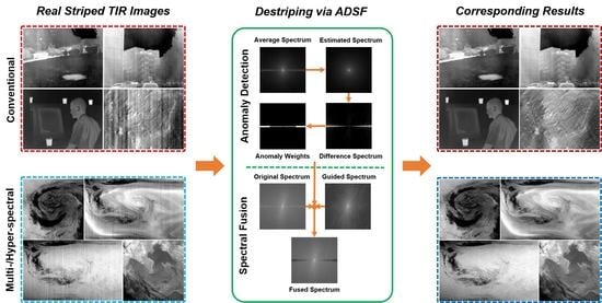
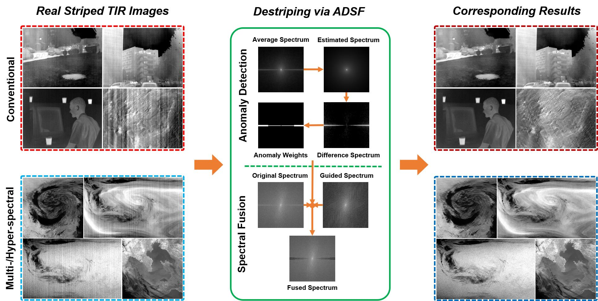
:Stripe noise is a common and unwelcome noise pattern in various thermal infrared (TIR) image data including conventional TIR images and remote sensing TIR spectral images. Most existing stripe noise removal (destriping) methods are often difficult to keep a good and robust efficacy in dealing with the real-life complex noise cases. In this paper, based on the intrinsic spectral properties of TIR images and stripe noise, we propose a novel two-stage transform domain destriping method called Fourier domain anomaly detection and spectral fusion (ADSF). Considering the principal frequencies polluted by stripe noise as outliers in the statistical spectrum of TIR images, our naive idea is first to detect the potential anomalies and then correct them effectively in the Fourier domain to reconstruct a desired destriping result. More specifically, anomaly detection for stripe frequencies is achieved through a regional comparison between the original spectrum and the expected spectrum that statistically follows a generalized Laplacian regression model, and then an anomaly weight map is generated accordingly. In the correction stage, we propose a guidance-image-based spectrum fusion strategy, which integrates the original spectrum and the spectrum of a guidance image via the anomaly weight map. The final reconstruction result not only has no stripe noise but also maintains image structures and details well. Extensive real experiments are performed on conventional TIR images and remote sensing spectral images, respectively. The qualitative and quantitative assessment results demonstrate the superior effectiveness and strong robustness of the proposed method.
1. Introduction
Thermal infrared (TIR) imagery has been an indispensable data resource in the remote sensing field because of the peculiarity of this spectrum [1]. Typically, satellite-based TIR images are widely used to investigate and monitor earth resources and environment by characterizing surface temperature and emissivity [2,3,4]. Conventional TIR cameras are increasingly mounted onto some low-cost aerial platforms like drones and airships to collect images for detection, identification and analysis missions [5,6,7]. In these available TIR data, however, raw images are frequently found to suffer from a distinctive noise pattern that manifests itself as vertical or horizontal stripes. This phenomenon not only results in the visual degradation of images but also affects the precision of the downstream processing.
1.1. Two Striped TIR Image Cases
In real TIR image data, there are two common cases with stripe noise: one is conventional TIR images that mostly come from uncooled infrared focal plane array (IRFPA)-based thermal imagers [8,9,10,11] and the other is remote sensing TIR spectral images that are captured by spaceborne/airborne imaging spectrometers [12,13,14,15]. For conventional TIR images, the presence of stripe noise is attributed to the nonuniform response of IRFPA detectors, which are typically designed with a column-shared readout circuit architecture [8,11]. From the sensor perspective, in practice, to eliminate the response errors between detector elements, the calibration-based nonuniformity correction (CNUC) technology could be applied in TIR imaging systems. But this does not necessarily ensure the complete disappearance of stripe noise in the image, such as when the CNUC operation is not performed well or its efficiency declines in the long term usage due to the variation of the response characteristics of detectors. As for remote sensing spectral images, the occurrence of the striping effect has a direct relationship with the work mechanism of imaging spectrometers, which record the one dimensional cross-track measurement by whiskbroom or pushbroom scanning while the observation in the other spatial dimension depends on the platform in-track motion [14]. Because of unavoidable interferences and errors during the scan imaging, stripes are generated in the cross-track direction of spectral images, although a series of radiometric calibration procedures are also performed beforehand [15].
Given the above two cases, the destriping task is essentially identical and necessary. So in this paper we focus on these striped TIR images and strive to provide an universal and efficient solution to improve their quality for further thermal applications.
1.2. Related Work
Over the past decades, plenty of stripe noise removal methods have been proposed, which fall into two broad categories: processing in the spatial domain and in the transform domain.Both processing technologies are developed by excavating and utilizing the inherent differences between stripe noise and image. And more attention is paid to the single image based destriping problem.
Spatial methods for destriping can be roughly divided into 1D-filtering-based methods [11,16,17], statistics-based methods [12,13,14,18,19,20], optimization-based methods [21,22,23,24,25,26,27,28,29,30], and deep-learning-based methods [31,32,33,34]. Currently, 1D-filtering-based methods are mainly performed on conventional TIR images, and their basic idea is to utilize 1D edge-preserving filters to progressively separate stripe noise from the contaminated image in horizontal and vertical directions. For example, Cao et al. successively used 1D row and column guided filters to achieve the estimation of stripe noise [16]. However, this method may produce some spurious artifacts near strong vertical edges, as has been demonstrated in [17]. Statistics-based methods, as one kind of classical correction methods, build on the similarity assumption of the data that global or local subscenes (or striping lines) should share the same statistics such as the histogram distribution [13,19], and the mean and standard deviation [12,14]. Such prerequisites are simple, efficient but idealistic, often resulting in an inadequate destriping effect in the complex real-world cases. For this reason, the combination of the statistics-based methods and other processing methods is becoming a practicable solution to balance the effectiveness and efficiency in real applications [15]. In recent years, optimization-based methods have been studied popularly owing to powerful model representation, excellent destriping result and flexible regularization strategy. In these optimization frameworks, the desired clean image is computed by minimizing an energy function with different regularization terms, which mathematically represent the prior knowledge of stripe noise and image. Bouali et al. considered the directional feature of stripes and proposed an unidirectional total variation (UTV) model to remove stripe noise while preserving image details [21]. Subsequently, many UTV variants are developed to further enhance the model’s adaptivity [22,23,24,25]. Other prior knowledge of stripes including low rank [26,27] and sparsity [28,29,30] are primely explored and applied in the relevant models as well. From a pragmatic perspective, these sophisticated optimization approaches tend to be multi-parametric and time-consuming, which makes them have lower utility. More recently, some deep-learning-based methods have emerged and created impressive destriping results, benefiting from the neural networks’ formidable function. In [22], Xiao et al. designed a nine-layered convolutional neural networks (CNNs) architecture for removing stripe noise from a single meteorological satellite infrared cloud image. He et al. added a polynomial simulation module of stripe noise into their CNNs training to improve networks’ discrimination ability of the noise [23]. So for these deep-learning-based methods, there may be two aspects worth considering to upgrade their performance; namely, enhancing the discrimination of stripe noise and the comprehension of image content [35]. The concrete challenges could include a realistic simulation model of stripe noise, a particular objective function (with some prior knowledge about the noise and image), an elaborate network architecture and so on.
As an alternative for destriping, transform domain methods that are chiefly designed and realized in the Fourier domain and wavelet domain have also received considerable attention and research [35,36,37,38,39,40,41,42,43,44]. One significant starting point of these methods is that stripe noise has a concentrated energy distribution in both domains due to its directionality and global similarity. Perhaps the most representative one among the transform domain methods is the combined method of wavelet-Fourier filtering [36,37]. It takes full advantage of the noise characteristics in the wavelet and Fourier domains to jointly filter out stripes while maintaining the detail information of image. Before this method, some simple filtering methods in the Fourier domain and wavelet domain had been proposed and achieved initial results [38,39,40,41]. Recently, researchers have introduced some advanced spatial processing techniques into transform domains and thus developed a number of state-of-the-art transform-based methods for destriping. In [42], a multi-scale operation of guided filtering is performed on the noisy wavelet coefficients to adaptively estimate stripe noise from vertical high-frequency details. One preliminary study of ours on destriping is to correct the dominant Fourier coefficients that are contaminated by stripe noise with a reference spectrum [43]. Moreover, the idea of deep learning is being integrated into the wavelet domain to produce possibly better destriping results [35,44].
1.3. Motivation
In this paper, we focus on the destriping task in the Fourier domain for TIR images. Early Fourier domain methods remove stripe noise by using simple 1D filters [36,37], and some newly related methods design adaptive 2D filters to accomplish the goal [45,46]. However, as many literatures pointed out, on the one hand, these naive filtering approaches have limited ability to handle stripes when faced with manifold real cases and most of them are in fact only available for periodic stripes; on the other hand, the methods may cause the so-called ringing artifact owing to the high discontinuity of image intensity and the blur of useful structure details that have the same frequencies as stripes. These drawbacks restrict the development of the Fourier domain destriping technique to some degree and make it fail to show a good competitiveness in processing real striped images. Therefore, this paper attempts to make some contributions and provide a new line of thought for Fourier domain based destriping methods.
To be specific, we propose a Fourier domain anomaly detection and spectral fusion method to remove stripe noise of TIR images. In this two-step framework, the abnormal frequencies that are likely to be contaminated by stripe noise are detected intentionally so that an anomaly weight map is generated to represent the information; then a fusion strategy between the original spectrum and the spectrum of a stripe-free guidance image is adopted to obtain the new corrected spectrum. Finally, the resultant image has no stripe noise while keeping the original structures and details well. Experimental results on conventional TIR images and remote sensing TIR spectral images fully demonstrate the superior destriping performance of the proposed method by comparing with other state-of-the-art destriping methods in both fields. The main idea and contributions of the proposed method are summarized as follows:
- The respective spectral characteristics of TIR images and stripe noise are explored systematically. On this basis, a Fourier domain anomaly detection method is proposed to locate the abnormal frequencies that are likely to be contaminated by stripe noise. As a result, an anomaly weight map is obtained.
- With the anomaly weight map, a fusion strategy between the original spectrum and the spectrum of a stripe-free guidance image is adopted to generate the new Fourier spectrum and then to reconstruct the destriped image. In the implementation, the guidance image is estimated via an adequate de-texture filter.
- Extensive experiments on real striped TIR data including conventional TIR images and remote sensing spectral images are performed. The results demonstrate that the proposed method has better destriping ability and stronger robustness, compared with the state-of-the-art destriping methods in the two fields.
The remainder of this paper is organized as follows. In Section 2, the spectral characteristics of TIR images and stripe noise are investigated. In Section 3, the proposed Fourier domain anomaly detection and spectral fusion method is described. In Section 4, we present the experimental results to validate the algorithm performance. Finally, conclusions are drawn in Section 5.
2. Spectral Analysis
2.1. Brief Reminder and Notations
In the Fourier theory of 2D image, the discrete Fourier transform (DFT) and the inverse discrete Fourier transform (IDFT) are defined as
where is a sized image and is its Fourier spectrum with the same size; and are spatial and spectral coordinates and have integer values; j is the imaginary unit. In practice, is often shifted so that the origin is at the center of the whole spectrum. Using , we denote the corresponding normalized frequencies by and (units are cycles per pixel) in each direction and thus . is the power spectrum of I.
In this work, since the representation of with the spatial frequency is involved, we also use the polar coordinate , where is the radial distance from and is the counter-clockwise angle from the or u-axis. So the spatial frequency is simply denoted by f without the directions. These notations will be unified in later parts.
2.2. Spectral Statistics of TIR Images
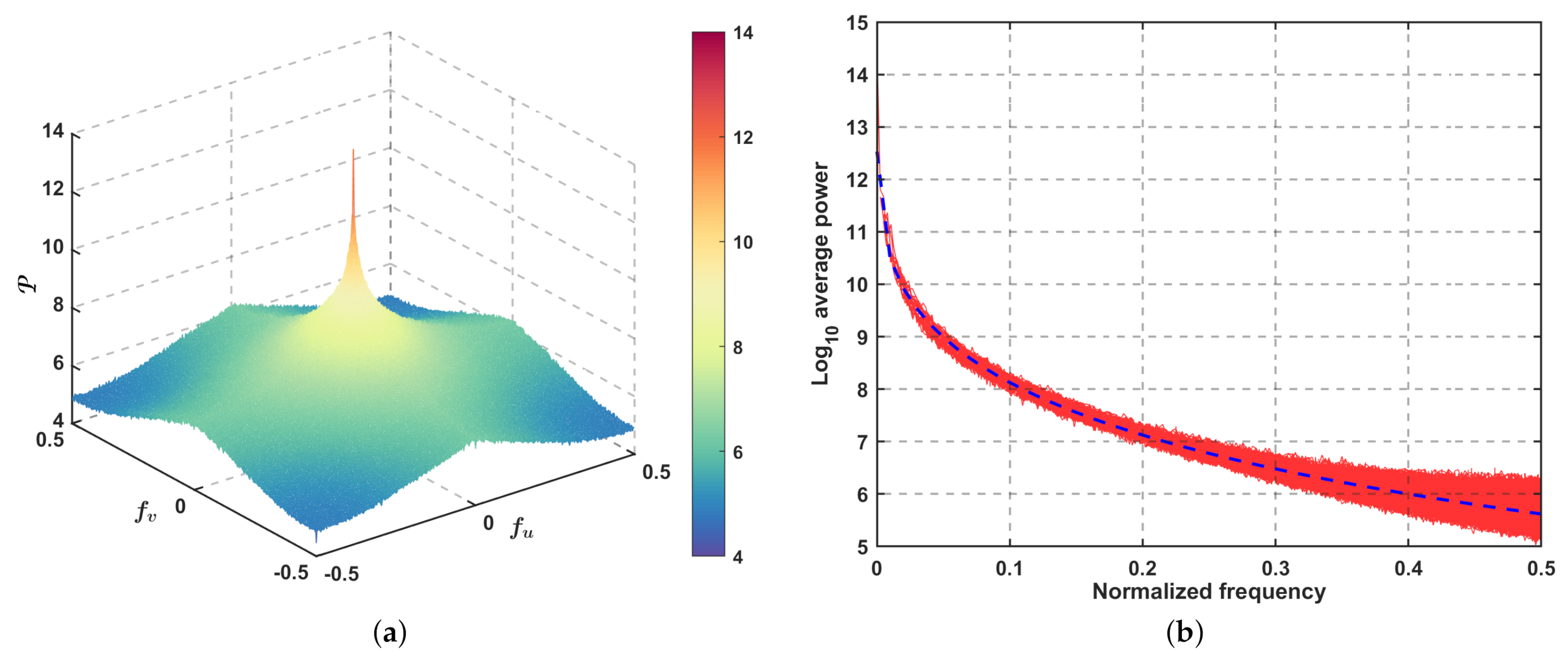
As is well known, the power spectrum of an image roughly obeys a power law , which has been widely applied to natural images [47,48,49]. However, the law may not be perfectly suited to TIR images. Morris et al. in the study of statistics of TIR images found that the average power spectra obtained from their TIR image datasets have increased DC and low-frequency components because of the relative lack of textural details in TIR images [50]. Considering this fact, the authors came up with a generalized Laplace distribution to model the average power of TIR images. It is expressed as
where a, b and c are the model parameters.
To revalidate this finding, we conducted the statistical test on a remote sensing TIR image dataset from [31], which is intentionally chosen to differ from Morris’s conventional TIR datasets. In detail, we first computed the average power spectrum of the dataset and then used the given Laplace model to fit it via the least squares method. Figure 1 shows the survey results, where the dotted curve is the fitted Laplacian distribution and the red part is the average power distribution. It can be seen that the fitted curve matches pretty well with the real distribution. This indicates the effectiveness of the Laplace model expressed in Equation (3). Hence, it is feasible to utilize the generalized Laplace distribution to represent the statistical power spectra of TIR images.
2.3. Spectral Distribution of Stripe Noise
It has been found that structural image components within a fixed direction have a directionally concentrated energy distribution in the Fourier domain and the two directions are orthogonal to each other. The spectral distribution of stripe noise follows this objective law due to its spatial directionality [51]. To further analyse and illustrate it, Figure 2 shows an experimental example where several common types of vertical stripes are given, including the periodic stripes, the non-periodic sparse stripes and the non-periodic non-sparse stripes. We can easily see from the example that the dominant frequencies affected by these vertical stripes are distributed in the horizontal centerline of image spectrums. For the periodic stripes, theoretically, their spectrum should be an ideal comb-like spectrum with only a few fixed frequencies, but as shown in Figure 2b, spectral leakage may occur in reality because of non-ideal periodicity [45]. For the non-periodic (sparse or non-sparse) stripes, their spectral energy evenly spreads to all frequencies [36,52], forming an arresting line as shown in Figure 2c,d. Precisely based on such spectral distribution characteristics, Fourier domain destriping methods can work effectively by detecting and suppressing the dominant noise frequencies. In addition, it’s worth noting that the power spectrum of the Pentagon image is actually a good proof of the above spatial-spectral law, where there are five obvious energy bands within different orientations corresponding to the five-sided structure in the image. This fact also implies a potential problem with the conventional Fourier domain destriping methods, that the image structure which has the same direction as stripe noise could be severely blurred because of the similar spectral distribution. Therefore, as has been stated in the introduction, how to reduce the stripe frequencies while protecting the structurally similar spectral information is an important and realistic issue for Fourier domain based destriping methods.
3. Methodology
In this paper, we focus on the destriping problem of TIR images in the Fourier domain and put forward an effective two-step solution called Fourier domain anomaly detection and spectral fusion (ADSF). Figure 3 is a schematic overview of the proposed method. The first step, anomaly detection, aims at identifying the abnormal Fourier coefficients that are dominantly contaminated by stripe noise. As a result, a weight map is generated to represent the abnormality of Fourier spectrum. The second step is to obtain a stripe-free correction spectrum by manipulating the detected anomalies. For this purpose, a guidance image based spectrum fusion strategy is adopted, which organically integrates the spectral information of both the original image and the guidance image. The final ”fused” image has no stripe noise while holding the original structure and detail information. In the following subsections, we will detail the two parts and some practical considerations in the proposed method.
3.1. Anomaly Detection
Our idea of anomaly detection is based on spectral characteristics of TIR images and stripe noise. As discussed in Section 2, on the one hand, the power spectrum of TIR images in natural statistics can be represented by a generalized Laplace distribution; on the other hand, the frequencies contaminated by stripe noise are relatively anomalous in the whole spectrum because of having high energy and a specific distribution area. For the purpose of this article, that means that the stripe frequencies could be easily detected by comparing the original spectrum with an adaptively estimated spectrum that follows the given Laplace distribution statistically. Driven by such a rough idea, a stripe frequency anomaly detector is reasonably designed. To be concrete, there are two main substeps in the implementation of anomaly detection. The first step is to statistically estimate the adaptive power spectrum for the original TIR image by using the Laplace model. The second step is to detect the stripe-related outliers by making a regional comparison between the real spectrum and the estimated spectrum. Figure 4 illustrates the whole implementation process.
3.1.1. Spectral Estimation
Given a striped TIR image I with size , we first extract the sliding subimages with size from I. If the sliding step is , the number of subimages is
where the ceil function. In the implementation, we fix and .
Statistically, the subimages denoted by constitute a sample set of I. After obtaining the corresponding power spectrums through DFT and a logarithmic transformation, the average power spectrum is easily calculated by
Regardless of few exceptional peaks due to stripe noise, the natural distribution for should behave as a generalized Laplace distribution. Based on this, is fitted with the function expressed in Equation (3) by least squares-based nonlinear regression to obtain the adaptive model parameters , and . So the estimated power spectrum is as follows
We consider as an adaptive reference spectrum so that the difference spectrum between and is essentially an indication of all statistical anomalies
3.1.2. Regional Detection
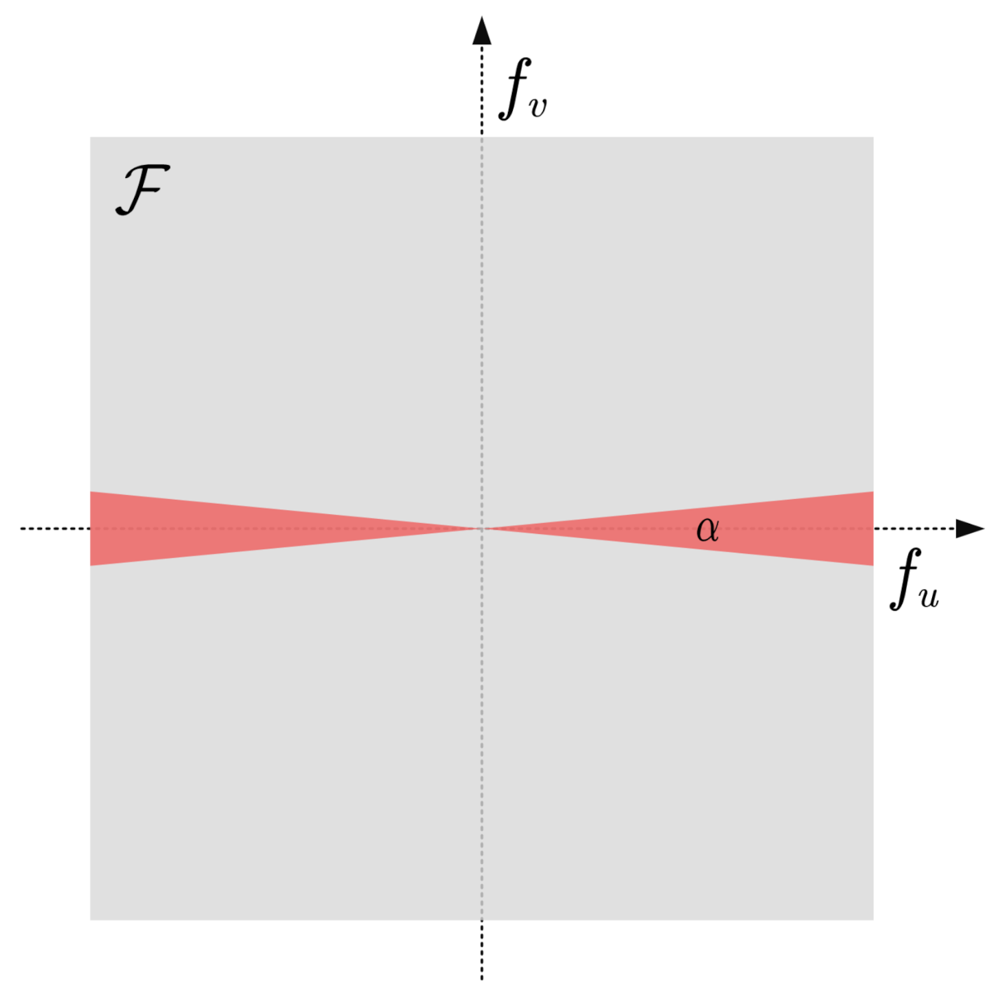
In order to further detect the anomalies caused by stripes in , a symmetric tapered slice is designated as the detection region of interest, according to the distribution rule of stripe frequencies. As shown in Figure 5, the size of the detection region depends on the taper angle having a small degree. Such design is based on a practical consideration that high-frequency abnormal components tend to be more than low-frequency abnormal components in most real cases. Without taking the DC component into account, can be defined as
Then, a thresholding operation is performed within to locate the stripe-related anomalies in . The initial anomaly map is obtained by
where stands for the threshold. It is determined via a simple rule where is the mean of at the spatial frequency f and t is set to 3 in the implementation.
The final anomaly weight map W is obtained from by two steps. First, we resize from to through the bilinear interpolation method. Subsequently, Gaussian filtering is carried out on the resized map to generate an ideal fusion weight map W. Like many conventional fusion methods, here the object of filtering is to repair some possible omissions around the anomalies in the initial weight map. The whole treatment process is formulated as
where ↑ and ⊗ are the interpolation and convolution operations, respectively. G is the Gaussian kernel and its size and standard deviation are set to and 2.
Although the dominant frequencies affected by stripe noise are effectively identified by anomaly detection, this does not mean that filtering out the anomalies simply is sufficient to achieve a good destriping result. Because some significant structure information also might lie behind these abnormal frequencies, as we discussed before. A better and more reasonable way is to repair the anomalies and obtain an adaptive corrected Fourier spectrum to reconstruct satisfactory destriping results. Therefore, a novel fusion-based spectrum correction approach is presented in the next section.
3.2. Guidance Image Based Spectrum Fusion
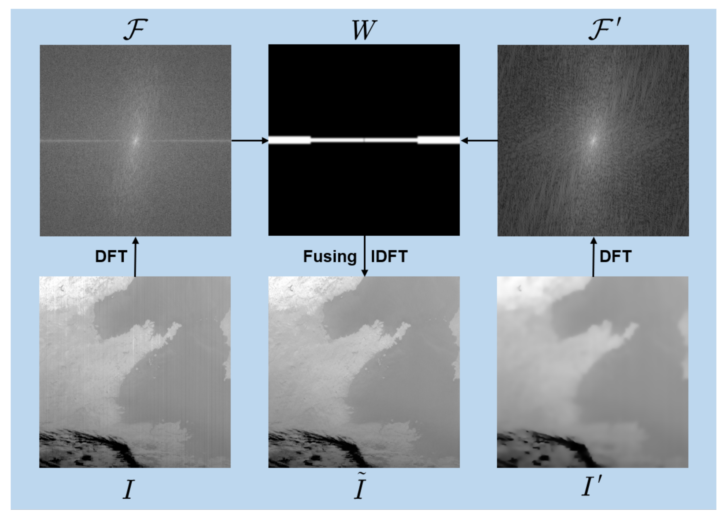
To adaptively correct the abnormality of Fourier spectrum due to stripe noise, we introduce the fusion principle into Fourier domain and propose a guidance image based spectrum fusion scheme. This approach not only achieves good and robust destriping results but also preserves more detail information, especially of some possible structures that are similar to stripes. Figure 6 shows the guidance image based spectrum fusion process. Its main idea is to fuse the Fourier spectrum of the original image with that of a guidance image via the anomaly weight map to obtain the corrected spectrum, thereby reconstructing a stripe-free but detail-preserved result. In the implementation, there are two basic links, generating a desired guidance image and then performing the spectrum fusion.
3.2.1. Guidance Image Generation
For the purpose of spectrum fusion, the guidance image is expected to be a smoothed version that has no stripe noise but keeps the original image information. Here we introduce an existing structure-texture decomposition technology called interval gradient filtering (IGF) [53] to obtain the desired guidance image. On the one hand, the IGF method decomposes images by adopting row-wise and column-wise filtering operations. The 1D filtering based mechanism is very effectual for stripe noise removal, as introduced in Section 1.2. On the other hand, since TIR images usually have more smooth homogeneous components and lower textural details, the IGF method is a perfectly suitable option for the estimation of the guidance image. Figure 7 gives an example of structure-texture decomposition via IGF on the striped image. We can see that the structural image used as a guidance image nicely retains the basic image content, but without any stripe noise. In the following, the fundamentals and implementation procedure of 1D IGF are concisely described.
For pixel k in a row signal R, the interval gradient is defined to measure the difference between the Gaussian weighted averages of the left and right parts in a k-centered window .
where and , respectively, stand for the right and left 1D Gaussian filtering with the standard deviation in . Compared with the common gradient , the interval gradient has an extremely important characteristic that if the window is texture-free. So the indicator (where is a small constant to prevent numerical instability) behaves that for structural regions and for textural regions. With this feature, an adaptive gradient rescaling rule is given, , to suppress textural gradients while retaining structural gradients.
Based on above concepts, the procedure of 1D IGF mainly comprises four steps: (1) calculating and of R; (2) rescaling to via the aforementioned rule; (3) reconstructing an initial filtered result by simply accumulating ; (4) Obtaining the final filtered result by filtering R with the guide of . Accordingly, 2D images are processed by alternately performing the 1D filtering operations in row and column directions. For more details about the IGF algorithm, please refer to the original paper.
By leveraging the IGF method on the original image I, the desired guidance image is generated.
3.2.2. Fourier Spectrum Fusion
With the guidance image and the anomaly weight map W, the corrected Fourier spectrum can be obtained by a fusion process
where ⊙ is the operator of element-wise multiplication; and are Fourier spectrums of I and , respectively.
Finally, the destriping result is reconstructed with via IDFT.
3.3. Practical Considerations
Because of some potentially negative effects in the Fourier domain processing of 2D image, which mainly include the so-called edge effect and ringing artifact [38], practical considerations are needed in the implementation of our algorithm to deal with these issues effectively.
The edge effect inevitably occurs when the Fourier transform is performed on discrete images, owing to strong discontinuities of image borders. As a result, a well-known cross structure made of high energy coefficients along the axes is formed in the Fourier spectrum. This could bring adverse impacts to the performance of the proposed method. To reduce the edge effect and ensure good reconstruction results, we adopt a dual preprocessing step: first, we expand the input image I to a larger size via an amount of padding in each dimension; and then a special method called periodic plus smooth decomposition is employed to decompose the expanded image into a periodic component (that is, an image resembling the original image but whose DFT does not suffer from the edge effect) and a smooth component that has very slow variations in the image domain [54]. So the resulting periodic image is used as the actual input image in our detection and fusion process.
In destriping results via DFT, the ringing artifacts resulting from the discontinuity of intensity in the image sometimes appear along the highly-contrasted edges [38]. As for our method, despite ideal Fourier coefficients from the guidance image to correct the spectrum, slight ringing artifacts might still be observed because of a mismatch between Fourier coefficients in the spectrum fusion. Thus, as an optional coping strategy, we introduce a spectrum interpolation method based on total variation minimization to mitigate these possible artifacts, which is originally applied in Fourier filtering methods [49,55]. Here we shall not detail the method, but to make it workable within the proposed framework, we define the spectrum region to be interpolated, , where the dominant Fourier coefficients in the fused spectrum are ruled out. More implementation details about the method can be found in the note of [55].
4. Experimental Results and Discussion
In this section, the performance of the proposed method is comprehensively evaluated. We focus on performing validations on two types of real-world TIR images we mentioned in Section 1.1, i.e., conventional TIR images and remote sensing TIR spectral images. To impartially demonstrate the effectiveness and robustness of our approach, abundant experiments are carried out on several publicly available datasets; at the same time, considering the differences of these two images in the research, we use the relevant contrast methods and common evaluation indexes for each case to compare and analyze the experimental results, respectively.
4.1. Experiments on Conventional TIR Images
For testing the proposed method on conventional TIR images, we utilize the open data coming from Tendero’s dataset (https://perso.telecom-paristech.fr/ytendero/) and Morris’s dataset (https://www.dgp.toronto.edu/~nmorris/IR/) and five state-of-the-art comparison methods including MIRE [19] (Midway Infrared Equalization), 1D-GF [16] (1D Guided Filtering), TwSF [52] (Two-Stage Filtering), DLSNUC [32] (Deep Learning-based Stripe Nonuniformity Correction), and WDNN [44] (Wavelet Deep Neural Network). Here three experiments are reported to illustrate the destriping performance of our method and their test images are shown in Figure 8. The images used in Experiments 1 and 2 are from Tendero’s dataset and record outdoor scenes at a resolution of 288 × 384, while the image used in Experiment 3 is an indoor image with size 288 × 384 and from Morris’s dataset. We can see that these real TIR images are obviously corrupted by vertical stripe noise.
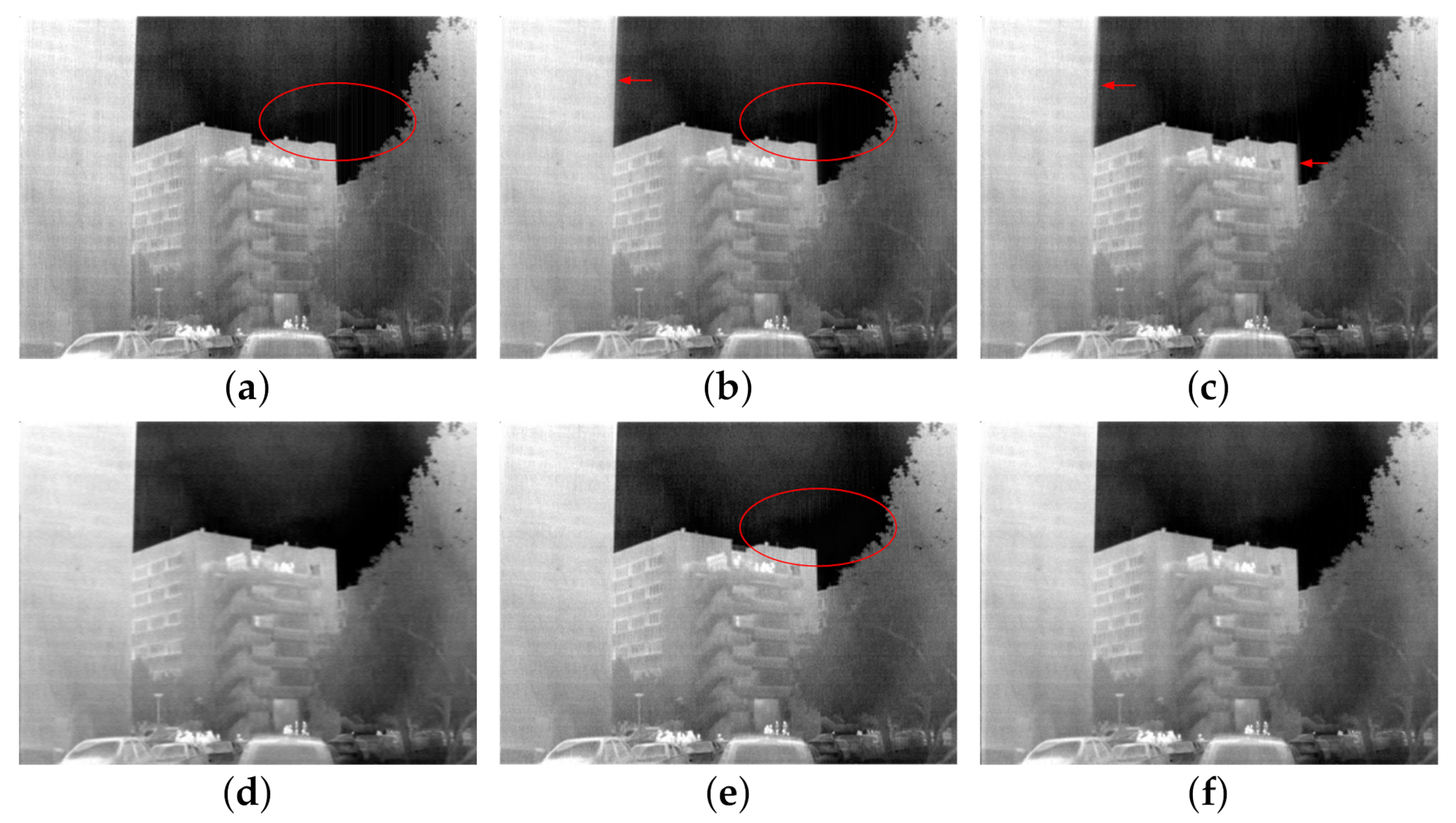
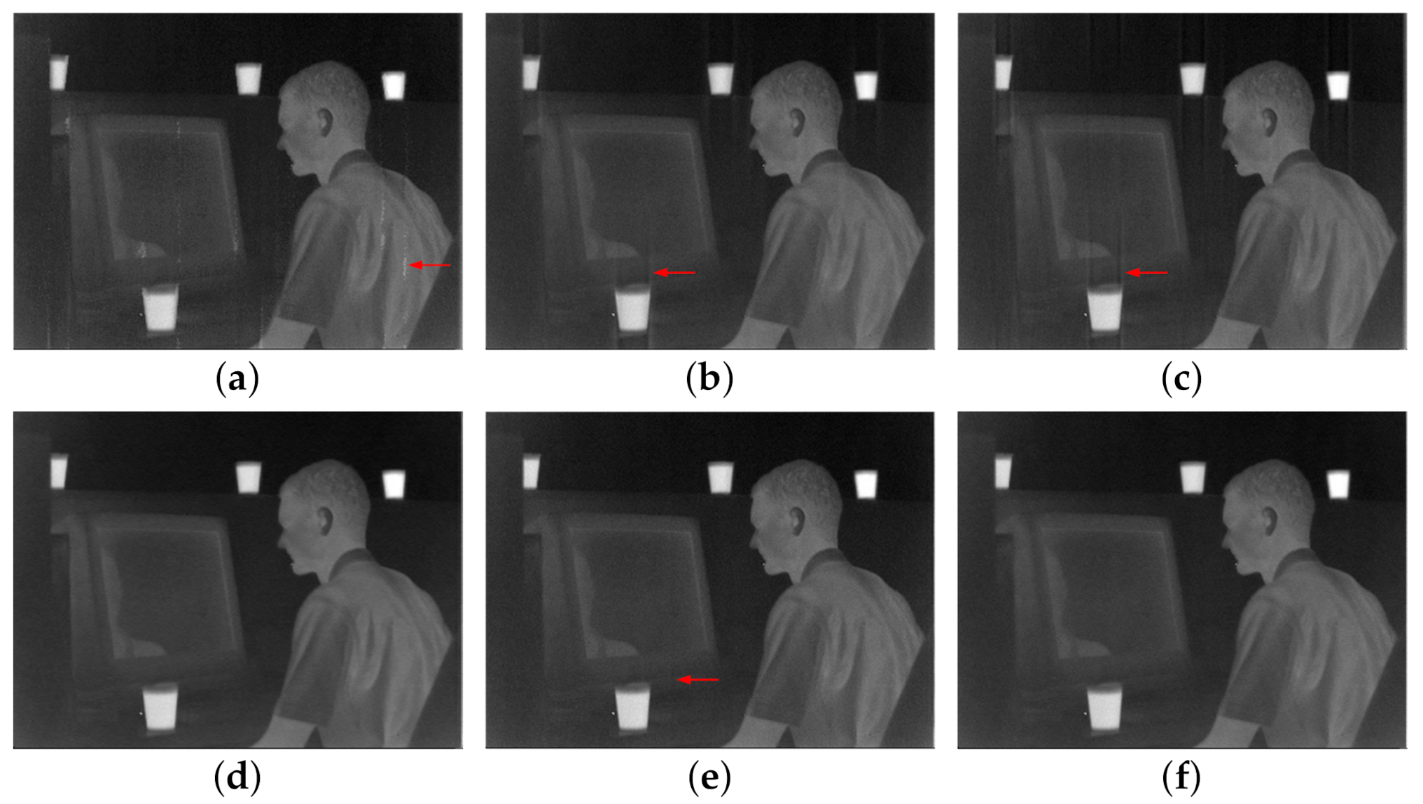
Figure 9, Figure 10 and Figure 11 show the destriping results of three experiments. From the first two groups of results, some slight stripes remain in the results of MIRE, 1D-GF and TwSF, such as in the labeled regions with red ovals in Figure 9c,d and Figure 10b,c. So these results look somewhat rough. Besides, in 1D-GF’s and TwSF’s results in Experiment 2, vertical structure edges (highlighted by red arrows in Figure 10c,d) are smoothed to some extent. The results produced by DLSNUC, WDNN and our method have a globally smooth and fine appearance with edge preservation. But from a local viewpoint, the stripe noise is not yet eliminated completely in certain areas of the WDNN’s result (see the red ovals in Figure 9f and Figure 10f). From the third group of results, we can find that there are some undesirable artifacts in the results of MIRE, GF, and TwSF, as marked with red arrows in Figure 11b–d. Some slight stripes are also observed in the WDNN’s result. By comparison, our method and DLSNUC achieve superior visual effects.
Further, as shown in Figure 12, we extract the pixels in a single row from each set of experimental results to comparatively analyse the performance of test methods in suppressing the noise as well as preserving the sharp changes of image details. The red arrows indicate some notable segments. Here we put focus on the comparison of DLSNUC, WDNN and the proposed method. From these results, DLSNUC has a stronger ability of smoothing the noise at the expense of some detailed information. WDNN is inclined to keep more original details, but this also means that the stripe noise may not be completely suppressed. In contrast, the proposed method is moderate, which can not only efficiently remove stripe noise but also preferably maintain image details.
To corroborate our observations in the qualitative comparison, an objective assessment is also made with four quantitative indicators and they are the roughness index [10], the smoothing difference index [11], the image content metric Q [56], and the root-mean-square error (RMSE), respectively. In TIR image quality assessment, is usually used to measure the smoothness of the whole image, defined as
where H and V are horizontal and vertical gradients of the image I, respectively; is the norm. A smaller value signifies a better smoothing effect. Another indicator is devoted to evaluating the algorithm’s ability in edge preservation and noise suppression by comparing the horizontal gradient smoothing difference between in structure and non-structure regions of TIR images, as follows
where H and correspond to horizontal gradients of images before and after destriping treatment; and are pixels in structure and non-structure regions, which are classified by the measurement of 1D horizontal differential statistics. generally yields positive values, with higher values indicating better edge-preserving effect while destriping. But if the value is less than 0, it suggests that some potential exceptions occur in the result. Since and essentially assess the image from a global perspective, we introduce the image patch based no-reference metric Q to locally evaluate the image quality. Concretely, the Q value of an image patch (with size by default) is computed by
where and are the first and second singular values of gradient matrix of the image patch. The mean Q value of all anisotropic patches is defined as the metric for the whole image. The higher the Q value is, the better quality the image has. What’s more, the error measurement RMSE is adopted to reflect the pixel accuracy of the destriped image. Its expression is
The quantitative evaluation results of three experiments for conventional TIR images are listed in Table 1. In terms of , DLSNUC has the lowest values, followed by our method and WDNN. This is in line with the conclusion in the qualitative analysis that our method does produce a moderately smooth result in between DLSNUC and WDNN. In respects of and Q, our method obtain the highest scores, illustrating its advantage in balancing between stripe noise removal and detail preservation. Moreover, the lowest RMSE values demonstrate that our method has better capability to hold the pixel accuracy of image when reducing stripe noise.
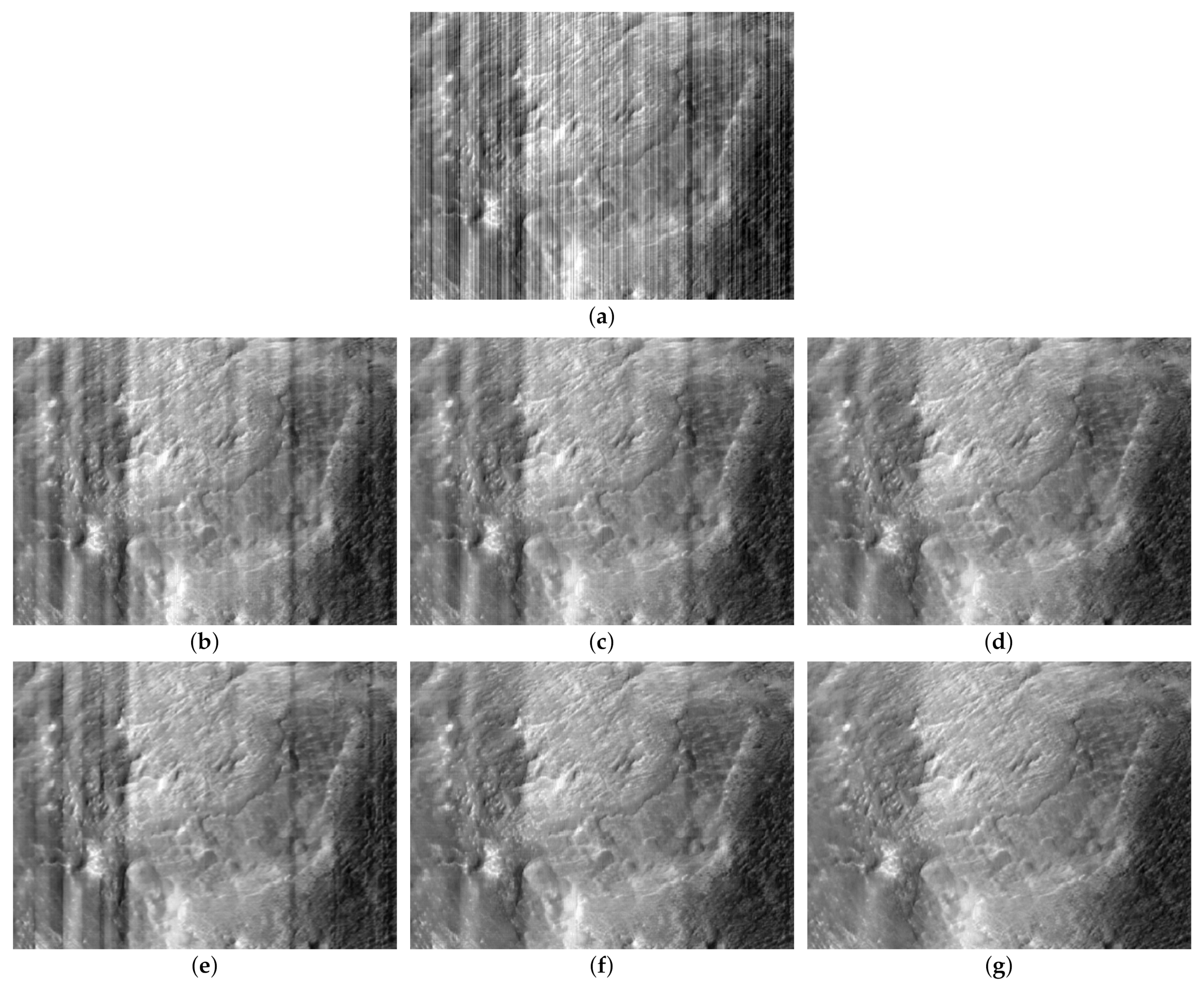
In our performance test, the extreme case that conventional TIR images are corrupted by very serious stripe noise is taken into consideration as well. Figure 13 provides one such example, where the test image is captured by Mars Orbiter satellite [44]. We can observe from the figure that there remain more or less striping effects in the other five results, compared to our result. This further reflects the practicability and superiority of the proposed method.
In summary, the proposed method exhibits the highly effective and robust destriping performance in a variety of real experiments on conventional TIR images.
4.2. Experiments on Remote Sensing Spectral Images
To demonstrate that our destriping approach is also applicable to remote sensing spectral images and has the consistently excellent performance, three sets of real striped multispectral data (see Figure 14), taken from Terra MODIS Level-1B products that are freely available on the website https://ladsweb.modaps.eosdis.nasa.gov, are tested with four pertinent methods for comparison. In Experiments 1 and 2, we separately selected a sequence of atmosphere images and land images within six TIR bands (Band 21, 24, 27, 33, 34 and 35), and they are extracted from the MOD021KM product and saved as 8-bit images with a cropped size of 500 × 500. From Figure 14, it can be seen that there are multiple types of stripes in these real spectral images: Band 21 and Band 24 images are degraded by periodically even stripes; Band 27 and Band 34 images suffer severely uneven stripes, while Band 33 and Band 35 images have mildly uneven stripes. The test data used in Experiment 3, including Band 27, 34 and 36 images, are collected from the MOD02SSH product and have a size of 270 × 406. In this group, the striping effect is remarkably inhomogeneous and mixed with some random noise, especially at Band 36. Additionally, the four single-image-based contrast methods for destriping of remote sensing images are as follows: WFAF [37] (Wavelet Fourier Adaptive Filtering), SLD [18] (Statistical Linear Destriping), LRSID [26] (Low Rank Single Image Decomposition), DSM- [30] (Directional Sparse Model).
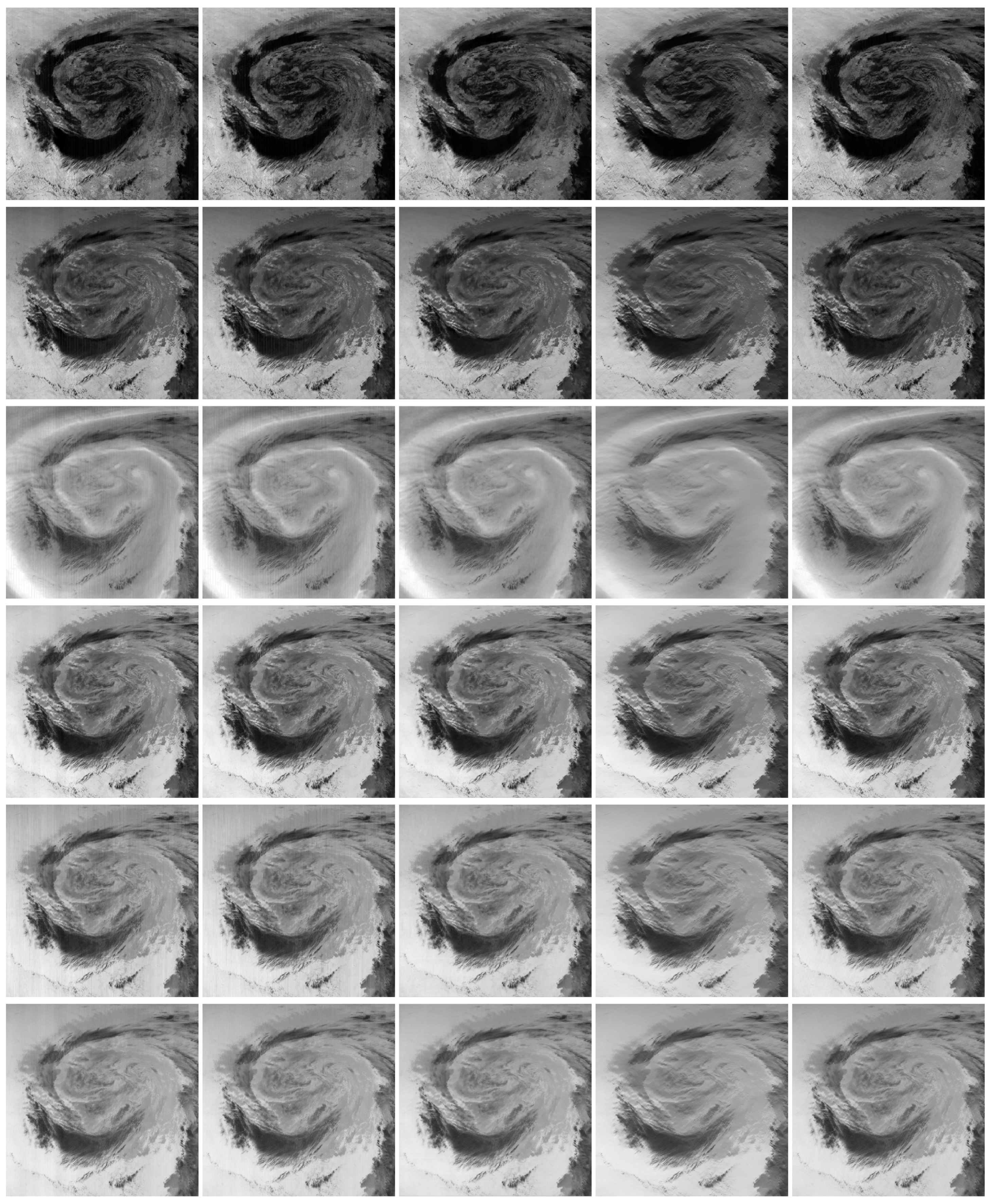
Figure 15, Figure 16 and Figure 17 show the destriping results of three experiments. Meanwhile for a better observation and comparison, we deliberately picked out a couple of image parts from the results of Experiments 1 and 2 to magnify and highlight visual differences, which are shown in Figure 18 and Figure 19. According to these results, some conclusions can be drawn. WFAF and SLD restrain stripes to certain extent, but their overall destriping effects are still inferior and many residual stripes are visible in their results. Also seeing from Experiment 2, WFAF could result in some light or shaded ribbonlike artifacts when there are a short, sharp variation in image contrast along the stripe direction. LRSID performs well in the case that the stripe in one column of image is steady and even, but its efficiency will deteriorate if the stripe case is less than ideal. For example, in dealing with the Band 27, 34 and 36 images, the results of LRSID are unsatisfactory because of fragmented and uneven stripes that are not perfectly fitted with the low rank prior, as the paper pointed out. DSM- has a good robust performance in the multifarious stripe cases, and its results are globally smooth without any stripes. However, such processing also causes the loss of a number of image detail information. The most notable cost is that many subtle gray changes are erased in image contents. By comparison, our approach unfurls a consistently impressive ability to work with various stripe cases, where not only are stripes effectively removed but also image details are well protected. It is especially noteworthy that, when the original image is damaged with a mix of stripes and random noise, the proposed method is still competent and achieves a better visual result than those of the other four algorithms, like the results of Band 36 showed in Figure 17.
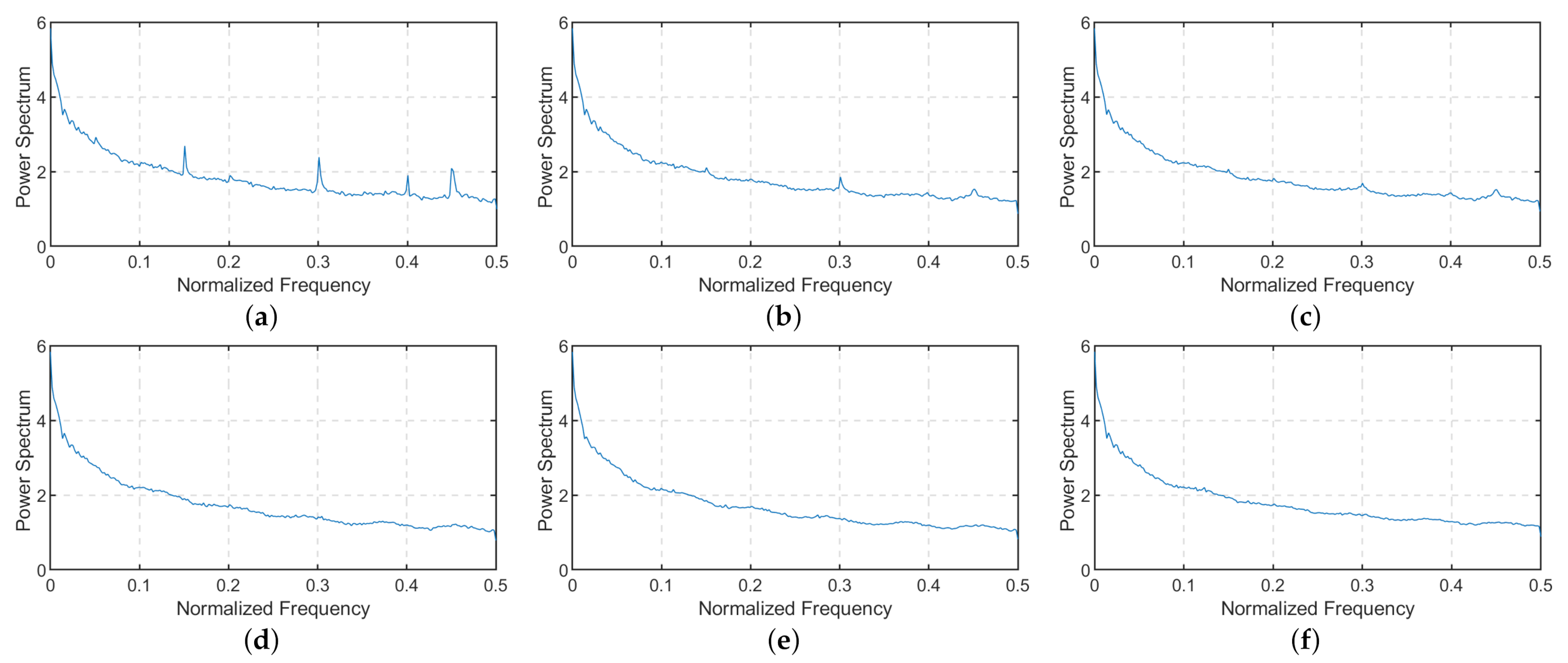
Also, we employ the mean cross-track profile and the mean row power spectrum to further verify the algorithm performance, which are two commonly qualitative analysis indicators for destriping of remote sensing images. Here the Band 21 image from Experiment 1 and the Band 27 image from from Experiment 2 are taken as example, and their mean cross-track profiles and mean row power spectrums are shown in Figure 20, Figure 21, Figure 22 and Figure 23. Generally, the mean cross-track profile of a good destriped result should be a smoothed version of that of the original image, with optimally preserving primary structure trends. But we can notice from Figure 20 and Figure 21 that the WFAF’s profile remains many obtrusive burrs, indicating a poor destriping effect. Conversely, the DSM-’s profile is over-smoothed and fails to keep some underlying image details well. The profiles of SLD, LRSID and the proposed approach have roughly semblable trends, but our result is more smooth than that of SLD and retains more finely structural fluctuations than that of LRSID. So in terms of the mean cross-track profile, the proposed method obtains the desired result both on smoothing stripes and maintaining image details. On the other hand, from the perspective of power spectrum (see Figure 22 and Figure 23), noise impulses are not reduced completely in the results of WFAF and SLD, while LRSID, DSM- and the proposed method produce similar and good results. Especially from Figure 23, after removing fragmentary and uneven stripes, the power spectrum of our result is more well-distributed with power preservation than other four methods.
To make a quantitative analysis of the above results, three frequently-used no-reference indices are introduced. Specifically, we adopt the inverse coefficient of variation (ICV) [13,14] and the mean relative deviation (MRD) [15] to assess the ability of destriping methods on balancing noise cancellation and detail preservation. The two indexes are defined as
where and are the mean and standard deviation of pixel values in a homogeneous region; and are the k-th pixel pair before and after destriping in a sharp region, and M is the total number of pixels. The ICV index is designed to measure the smoothness of a homogeneous region, while the MRD index reflects the relative distortion of a sharp region. So a good destriping performance should be the combination of a large ICV value and a small MRD value. Apart from evaluating in the dimension of image, we also give consideration to the influence of the destriping operation on the spectral fidelity. Here the common metric in the spectral imaging filed, spectral angle mapper (SAM) [57,58], is utilized to numerically evaluate the distortion between the original and destriped spectral signatures. Its definition is as follows
where and stand for the k-th spectral signatures of the original and destriped spectral images, respectively. In general, the smaller the SAM value is, the less the distortion is between and .
Table 2 lists the ICV, MRD and SAM values of all the destriped spectral bands from Experiments 1 and 2. In terms of ICV and MRD indexes, it can be found that, DSM- achieves not only all the largest ICV values but also the largest MRD values, while WFAF and SLD are in the opposite situation, corresponding to the smallest ICV and MRD values alternately. Both results are unacceptable because they actually indicate the oversmoothing effect of DSM- and the undersmoothing effect of WFAF and SLD, combined with the visual results. By comparison, LRSID and the proposed method obtain modest, balanced ICV and MRD values for six bands. But the proposed method has higher ICV values and lower MRD values than LRSID in Band 27 and Band 34 where the stripe noise is severe and irregular. It shows the better coping capacity of the proposed method in these two cases. So judging from the results of ICV and MRD, our method reaches a good and robust trade-off between stripe noise suppression and detail preservation. In addition, from the SAM perspective, the proposed method gets the lowest values, which means that the spectral distortion caused by the method is slightest, compared with other destriping methods.
Overall, for remote sensing spectral images, the proposed method also can maintain the stable and competitive destriping performance with minimum loss of the spatial-spectral information.
4.3. Discussion
4.3.1. Parameter Analysis
In the implementation of the proposed method, there are two tunable parameters that significantly affect performance, the taper angle and the standard deviation . Specifically, determines the size of the tapered detection region in the stage of anomaly detection. So when is tuned from a small degree to a relatively large degree, it means that more potential high-frequency anomalies may be detected and restrained. To illustrate the influence of the parameter on the destriping performance, Figure 24 gives an example, where the original image has even stripes as well as some uneven fragmented stripes, such as in the area marked with a red square. From the destriping results with different values, we can find that, when has a small degree (∼6), the even regular stripes are removed well but the uneven fragmented stripes still remain in local areas; all stripes are suppressed when is set to a relatively large degree (∼16). Thus a large is favorable for the given case. On the contrary, for most general cases, a small is sufficient and suggested because more detailed information could be saved. In our implementation, is fixed as by default.
The other parameter regulates the generation of the guidance image in the stage of spectrum fusion. Actually, is involved in the IGF method [53] and it determines the degree of filtering, that is, the filtered image becomes more smooth as increases. Since the guidance image is supposed to be a stripe-free base image, has to be properly adjusted with the level of actual stripe noise in the implementation of our approach. For most general cases, is set in the range of 0.5∼3. It should be noted that, on the premise of ensuring the guidance image without stripes, a small is suggested so that the guidance image keeps more fine details, which could be fused into the result.
4.3.2. Running Time
We also consider running times of different methods to examine their computation complexity. In this paper, all the experiments are conducted on a laptop personal computer with an Intel Core 2.4-GHz CPU and 8-GB RAM and the codes of algorithms are implemented in Matlab expect WDNN in Python. Table 3 records the average running times of different methods in experiments on conventional TIR images with size 288 × 384 and remote sensing spectral images with size 500 × 500. It can be concluded that statistics-based methods like MIRE and SLD and filtering-based methods such as 1D-GF, TwSF and WFAF are relatively simple and have the low cost of computation; while optimization-based methods like LRSID and DSM- and deep-learning-based methods including DLSNUC and WDNN are usually complicated and require a large quantity of operation. By comparison, the time consumption of our method is modest and acceptable.
5. Conclusions
In this paper, we have proposed a novel Fourier domain anomaly detection and spectral fusion approach for the destriping of TIR imagery. First, based on spectral characteristics of both TIR images and stripe noise, the abnormal frequencies that are likely to be caused by stripe noise are detected to generate an anomaly weight map. With this map, the original spectrum is then fused with the spectrum of a guidance image, which is estimated by a proper de-texture filter. As a result, in the ”fused” image, not only is the stripe noise removed effectively, but original structures and details are preserved well. Lots of experiments are performed on two types of real striped TIR data including conventional TIR images and remote sensing spectral images. Both qualitative and quantitative results demonstrate the excellent destriping performance of the proposed method with less loss of the original information, compared with the other state-of-the-art destriping methods in the two fields.
Author Contributions
Q.Z. designed the algorithm, made the experiments and wrote the manuscript; H.Q. assisted in the prepared work; X.Y. discussed the results; T.Y. gave some comments. All authors contributed to the improvement of the manuscript’s presentation. All authors have read and agreed to the published version of the manuscript.
Funding
This research was funded by the National Natural Science Foundation of China (No. 61901330), the China Postdoctoral Science Foundation (No. 2019M653566), and the Natural Science Foundation of Shaanxi Province (No. 2020JQ-322).
Acknowledgments
The authors would like to thank the China Scholarship Council for their financial support and help.
Conflicts of Interest
The authors declare no conflict of interest.
References
- Sobrino, J.A.; Del Frate, F.; Drusch, M.; Jiménez-Muñoz, J.C.; Manunta, P.; Regan, A. Review of thermal infrared applications and requirements for future high-resolution sensors. IEEE Trans. Geosci. Remote Sens. 2016, 54, 2963–2972. [Google Scholar]
- Tronin, A.A.; Hayakawa, M.; Molchanov, O.A. Thermal IR satellite data application for earthquake research in Japan and China. J. Geodyn. 2002, 33, 519–534. [Google Scholar]
- Blackett, M. An overview of infrared remote sensing of volcanic activity. J. Imaging 2017, 3, 13. [Google Scholar]
- Chen, Y.; Duan, S.; Ren, H.; Labed, J.; Li, Z. Algorithm development for land surface temperature retrieval: Application to Chinese Gaofen-5 data. Remote Sens. 2017, 9, 161. [Google Scholar]
- Stark, B.; Smith, B.; Chen, Y. Survey of thermal infrared remote sensing for unmanned aerial systems. In Proceedings of the IEEE International Conference on Unmanned Aircraft Systems (ICUAS), Orlando, FL, USA, 27–30 May 2014; pp. 1294–1299. [Google Scholar]
- Ren, P.; Meng, Q.; Zhang, Y.; Zhao, L.; Yuan, X.; Feng, X. An unmanned airship thermal infrared remote sensing system for low-altitude and high spatial resolution monitoring of urban thermal environments integration and an experiment. Remote Sens. 2015, 7, 14259–14275. [Google Scholar]
- Rahaghi, A.I.; Lemmin, U.; Sage, D.; Barry, D.A. Achieving high-resolution thermal imagery in low-contrast lake surface waters by aerial remote sensing and image registration. Remote Sens. Environ. 2019, 221, 773–783. [Google Scholar]
- Qian, W.; Chen, Q.; Gu, G.; Guan, Z. Correction method for stripe nonuniformity. Appl. Opt. 2010, 49, 1764–1773. [Google Scholar]
- Cao, Y.; Li, Y. Strip non-uniformity correction in uncooled long-wave infrared focal plane array based on noise source characterization. Opt. Commun. 2015, 339, 236–242. [Google Scholar]
- Goodall, T.R.; Bovik, A.C.; Paulter, N.G. Tasking on natural statistics of infrared images. IEEE Trans. Image Process. 2016, 25, 65–79. [Google Scholar]
- Cao, Y.; He, Z.; Yang, J.; Cao, Y.; Yang, M.Y. Spatially adaptive column fixed-pattern noise correction in infrared imaging system using 1D horizontal differential statistics. IEEE Photonics J. 2017, 9, 1–13. [Google Scholar]
- Gadallah, F.L.; Csillag, F.; Smith, E.J.M. Destriping multisensor imagery with moment matching. Int. J. Remote Sens. 2000, 21, 2505–2511. [Google Scholar]
- Rakwatin, P.; Takeuchi, W.; Yasuoka, Y. Stripe noise reduction in MODIS data by combining histogram matching with facet filter. IEEE Trans. Geosci. Remote Sens. 2007, 45, 1844–1856. [Google Scholar]
- Kang, Y.; Pan, L.; Sun, M.; Liu, X.; Chen, Q. Destriping high-resolution satellite imagery by improved moment matching. Int. J. Remote Sens. 2017, 38, 6346–6365. [Google Scholar]
- Jia, J.; Wang, Y.; Cheng, X.; Yuan, L.; Zhao, D.; Ye, Q.; Zhuang, X.; Shu, R.; Wang, J. Destriping algorithms based on statistics and spatial filtering for visible-to-thermal infrared pushbroom hyperspectral imagery. IEEE Trans. Geosci. Remote Sens. 2019, 57, 4077–4091. [Google Scholar]
- Cao, Y.; Yang, M.Y.; Tisse, C.L. Effective strip noise removal for low-textured infrared images based on 1-D guided filtering. IEEE Trans. Circuits Syst. Video Technol. 2016, 26, 2176–2188. [Google Scholar]
- Li, F.; Zhao, Y.; Xiang, W. Single-frame-based column fixed-pattern noise correction in an uncooled infrared imaging system based on weighted least squares. Appl. Opt. 2019, 58, 9141–9153. [Google Scholar]
- Carfantan, H.; Idier, J. Statistical linear destriping of satellite-based pushbroom-type images. IEEE Trans. Geosci. Remote Sens. 2010, 48, 1860–1871. [Google Scholar]
- Tendero, Y.; Landeau, S.; Gilles, J. Non-uniformity correction of infrared images by midway equalization. Image Process. Line 2012, 2, 134–146. [Google Scholar]
- Shen, H.; Jiang, W.; Zhang, H.; Zhang, L. A piece-wise approach to removing the nonlinear and irregular stripes in MODIS data. Int. J. Remote Sens. 2014, 35, 44–53. [Google Scholar]
- Bouali, M.; Ladjal, S. Toward optimal destriping of MODIS data using a unidirectional variational model. IEEE Trans. Geosci. Remote Sens. 2011, 49, 2924–2935. [Google Scholar]
- Chang, Y.; Fang, H.; Yan, L.; Liu, H. Robust destriping method with unidirectional total variation and framelet regularization. Opt. Express 2013, 21, 23307–23323. [Google Scholar] [CrossRef] [PubMed]
- Wang, M.; Zheng, X.; Pan, J.; Wang, B. Unidirectional total variation destriping using difference curvature in MODIS emissive bands. Infrared Phys. Technol. 2016, 75, 1–11. [Google Scholar] [CrossRef]
- Huang, Y.; He, C.; Fang, H.; Wang, X. Iteratively reweighted unidirectional variational model for stripe non-uniformity correction. Infrared Phys. Technol. 2016, 75, 107–116. [Google Scholar] [CrossRef]
- Boutemedjet, A.; Deng, C.; Zhao, B. Edge-aware unidirectional total variation model for stripe non-uniformity correction. Sensors 2018, 18, 1164. [Google Scholar] [CrossRef] [PubMed] [Green Version]
- Chang, Y.; Yan, L.; Wu, T.; Zhong, S. Remote sensing image stripe noise removal: From image decomposition perspective. IEEE Trans. Geosci. Remote Sens. 2016, 54, 7018–7031. [Google Scholar] [CrossRef]
- Yang, J.; Zhao, X.; Ma, T.; Chen, Y.; Huang, T.; Ding, M. Remote sensing images destriping using unidirectional hybrid total variation and nonconvex low-rank regularization. J. Comput. Appl. Math. 2020, 363, 124–144. [Google Scholar] [CrossRef]
- Liu, X.; Lu, X.; Shen, H.; Yuan, Q.; Jiao, Y.; Zhang, L. Stripe noise separation and removal in remote sensing images by consideration of the global sparsity and local variational properties. IEEE Trans. Geosci. Remote Sens. 2016, 54, 3049–3060. [Google Scholar] [CrossRef]
- Chen, Y.; Huang, T.; Deng, L.; Zhao, X.; Wang, M. Group sparsity based regularization model for remote sensing image stripe noise removal. Neurocomputing 2017, 267, 95–106. [Google Scholar] [CrossRef]
- Dou, H.; Huang, T.; Deng, L.; Zhao, X.; Huang, J. Directional l0 sparse modeling for image stripe noise removal. Remote Sens. 2018, 10, 361. [Google Scholar] [CrossRef] [Green Version]
- Xiao, P.; Guo, Y.; Zhuang, P. Removing stripe noise from infrared cloud images via deep convolutional networks. IEEE Photonics J. 2018, 10, 1–14. [Google Scholar] [CrossRef]
- He, Z.; Cao, Y.; Dong, Y.; Yang, J.; Cao, Y.; Tisse, C.L. Single-image-based nonuniformity correction of uncooled long-wave infrared detectors: A deep-learning approach. Appl. Opt. 2018, 57, D155–D164. [Google Scholar] [CrossRef] [PubMed]
- Chang, Y.; Yan, L.; Liu, L.; Fang, H.; Zhong, S. Infrared aerothermal nonuniform correction via deep multiscale residual network. IEEE Geosci. Remote Sens. Lett. 2019, 16, 1120–1124. [Google Scholar] [CrossRef]
- Guan, J.; Lai, R.; Xiong, A.; Liu, Z.; Gu, L. Fixed pattern noise reduction for infrared images based on cascade residual attention CNN. Neurocomputing 2020, 377, 301–313. [Google Scholar] [CrossRef] [Green Version]
- Chang, Y.; Chen, M.; Yan, L.; Zhao, X.L.; Li, Y.; Zhong, S. Toward universal stripe removal via wavelet-based deep convolutional neural network. IEEE Trans. Geosci. Remote Sens. 2019, 58, 2880–2897. [Google Scholar] [CrossRef]
- Münch, B.; Trtik, P.; Marone, F.; Stampanoni, M. Stripe and ring artifact removal with combined wavelet-Fourier filtering. Opt. Express 2009, 17, 8567–8591. [Google Scholar] [CrossRef] [Green Version]
- Pande-Chhetri, R.; Abd-Elrahman, A. De-striping hyperspectral imagery using wavelet transform and adaptive frequency domain filtering. ISPRS J. Photogramm. Remote Sens. 2011, 66, 620–636. [Google Scholar] [CrossRef]
- Pan, J.J.; Chang, C.I. Destriping of Landsat MSS images by filtering techniques. Photogramm. Eng. Remote Sens. 1992, 58, 1417. [Google Scholar]
- Chen, J.; Shao, Y.; Guo, H.; Wang, W.; Zhu, B. Destriping CMODIS data by power filtering. IEEE Trans. Geosci. Remote Sens. 2003, 41, 2119–2124. [Google Scholar] [CrossRef]
- Torres, J.; Infante, S.O. Wavelet analysis for the elimination of striping noise in satellite images. Opt. Eng. 2001, 40, 1309–1314. [Google Scholar]
- Yang, Z.; Li, J.; Menzel, W.P.; Frey, R.A. Destriping for MODIS data via wavelet shrinkage. Proc. SPIE Appl. Weather Satell. 2003, 4895, 187–199. [Google Scholar]
- Cao, Y.; He, Z.; Yang, J.; Ye, X.; Cao, Y. A multi-scale non-uniformity correction method based on wavelet decomposition and guided filtering for uncooled long wave infrared camera. Signal Process. Image Commun. 2018, 60, 13–21. [Google Scholar] [CrossRef]
- Zeng, Q.; Qin, H.; Yan, X.; Zhou, H. Fourier spectrum guidance for stripe noise removal in thermal infrared imagery. IEEE Geosci. Remote Sens. Lett. 2019, 17, 1072–1076. [Google Scholar] [CrossRef]
- Guan, J.; Lai, R.; Xiong, A. Wavelet deep neural network for stripe noise removal. IEEE Access 2019, 7, 44544–44554. [Google Scholar] [CrossRef]
- Pei, J.; Zou, M.; Zhao, Y. Adaptive comb-type filtering method for stripe noise removal in infrared images. J. Electron. Imaging 2019, 28, 013037. [Google Scholar] [CrossRef]
- Lin, J.; Zuo, H.; Ye, Y.; Liao, X. Histogram-based autoadaptive filter for destriping NDVI imagery acquired by UAV-loaded multispectral camera. IEEE Geosci. Remote Sens. Lett. 2019, 16, 648–652. [Google Scholar] [CrossRef]
- Field, D.J. Relations between the statistics of natural images and the response properties of cortical cells. J. Opt. Soc. Am. A 1987, 4, 2379–2394. [Google Scholar] [CrossRef] [Green Version]
- Yeganeh, H.; Rostami, M.; Wang, Z. Objective quality assessment for image super-resolution: A natural scene statistics approach. In Proceedings of the IEEE International Conference on Image Processing (ICIP), Orlando, FL, USA, 30 September–3 October 2012; pp. 1481–1484. [Google Scholar]
- Sur, F.; Grediac, M. Automated removal of quasiperiodic noise using frequency domain statistics. J. Electron. Imaging 2015, 24, 013003. [Google Scholar] [CrossRef]
- Morris, N.J.; Avidan, S.; Matusik, W.; Pfister, H. Statistics of infrared images. In Proceedings of the IEEE Conference on Computer Vision and Pattern Recognition (CVPR), Minneapolis, MN, USA, 17–22 June 2007; pp. 1–7. [Google Scholar]
- Liu, X.; Lu, X.; Shen, H.; Yuan, Q.; Zhang, L. Oblique stripe removal in remote sensing images via oriented variation. arXiv 2018, arXiv:1809.02043. [Google Scholar]
- Zeng, Q.; Qin, H.; Yan, X.; Yang, S.; Yang, T. Single infrared image-based stripe nonuniformity correction via a two-stage filtering method. Sensors 2018, 18, 4299. [Google Scholar] [CrossRef] [Green Version]
- Lee, H.; Jeon, J.; Kim, J.; Lee, S. Structure-texture decomposition of images with interval gradient. Comput. Graph. Forum 2017, 36, 262–274. [Google Scholar] [CrossRef]
- Moisan, L. Periodic plus smooth image decomposition. J. Math. Imaging Vis. 2011, 39, 161–179. [Google Scholar] [CrossRef] [Green Version]
- Sur, F. An a-contrario approach to quasi-periodic noise removal. In Proceedings of the IEEE International Conference on Image Processing (ICIP), Quebec City, QC, Canada, 27–30 September 2015; pp. 3841–3845. [Google Scholar]
- Zhu, X.; Milanfar, P. Automatic parameter selection for denoising algorithms using a no-reference measure of image content. IEEE Trans. Image Process. 2010, 19, 3116–3132. [Google Scholar] [PubMed]
- Yuan, Y.; Zheng, X.; Lu, X. Spectral–spatial kernel regularized for hyperspectral image denoising. IEEE Trans. Geosci. Remote Sens. 2015, 53, 3815–3832. [Google Scholar] [CrossRef]
- Lu, T.; Li, S.; Fang, L.; Ma, Y.; Benediktsson, J.A. Spectral–spatial adaptive sparse representation for hyperspectral image denoising. IEEE Trans. Geosci. Remote Sens. 2016, 54, 373–385. [Google Scholar] [CrossRef]
Figure 1.
Spectral statistics of TIR images. (a) Average power spectrum of the TIR image dataset from [31]; (b) Fitted result via the generalized Laplacian distribution.
Figure 1.
Spectral statistics of TIR images. (a) Average power spectrum of the TIR image dataset from [31]; (b) Fitted result via the generalized Laplacian distribution.

Figure 2.
Spectral distribution of stripe noise. (a) Pentagon image and power spectrum; (b) Pentagon image with periodic stripes and power spectrum; (c) Pentagon image with non-periodic sparse stripes and power spectrum; (d) Pentagon image with non-periodic non-sparse stripes and power spectrum.
Figure 2.
Spectral distribution of stripe noise. (a) Pentagon image and power spectrum; (b) Pentagon image with periodic stripes and power spectrum; (c) Pentagon image with non-periodic sparse stripes and power spectrum; (d) Pentagon image with non-periodic non-sparse stripes and power spectrum.
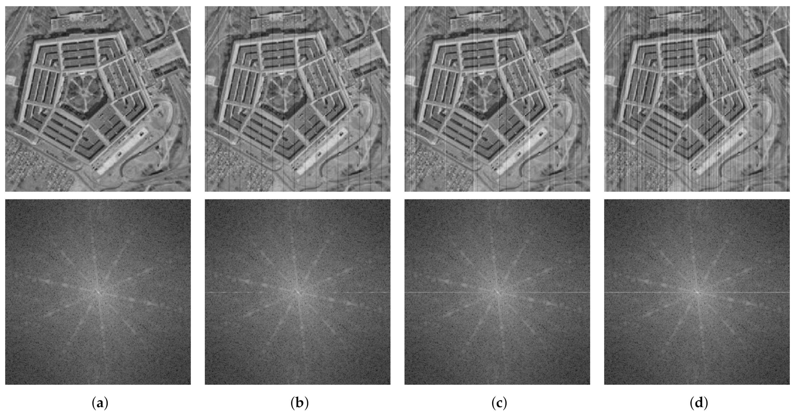
Figure 3.
A schematic overview of the proposed method.
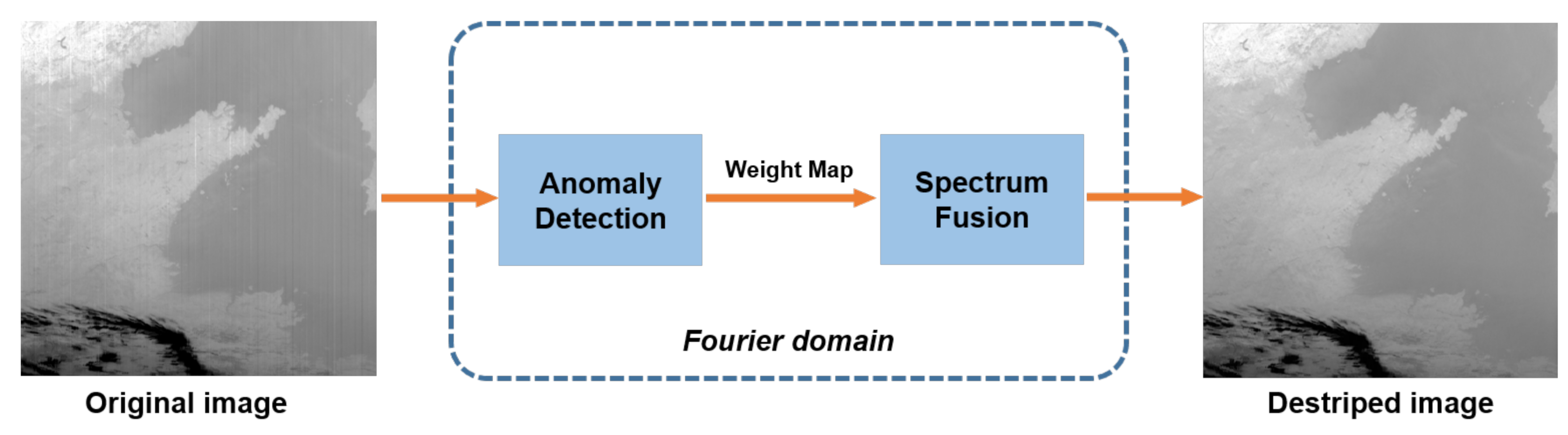
Figure 4.
The implementation process of anomaly detection.
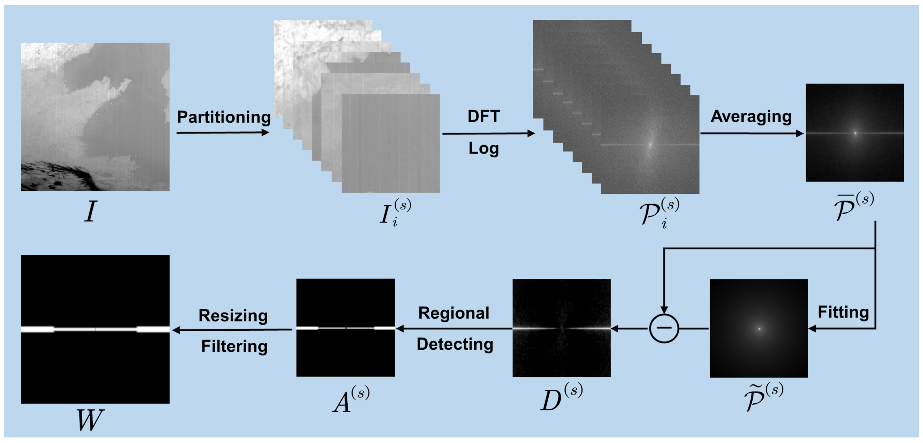
Figure 5.
A symmetric tapered region for stripe-related anomaly detection.

Figure 6.
The implementation process of spectrum fusion.

Figure 7.
Structure-texture decomposition via IGF on the striped image. (a) Original image; (b) Structural image used as a guidance image; (c) Textural image with stripe noise.
Figure 7.
Structure-texture decomposition via IGF on the striped image. (a) Original image; (b) Structural image used as a guidance image; (c) Textural image with stripe noise.

Figure 8.
Conventional TIR images used in the three experiments. (a) Experiment 1; (b) Experiment 2; (c) Experiment 3.
Figure 8.
Conventional TIR images used in the three experiments. (a) Experiment 1; (b) Experiment 2; (c) Experiment 3.
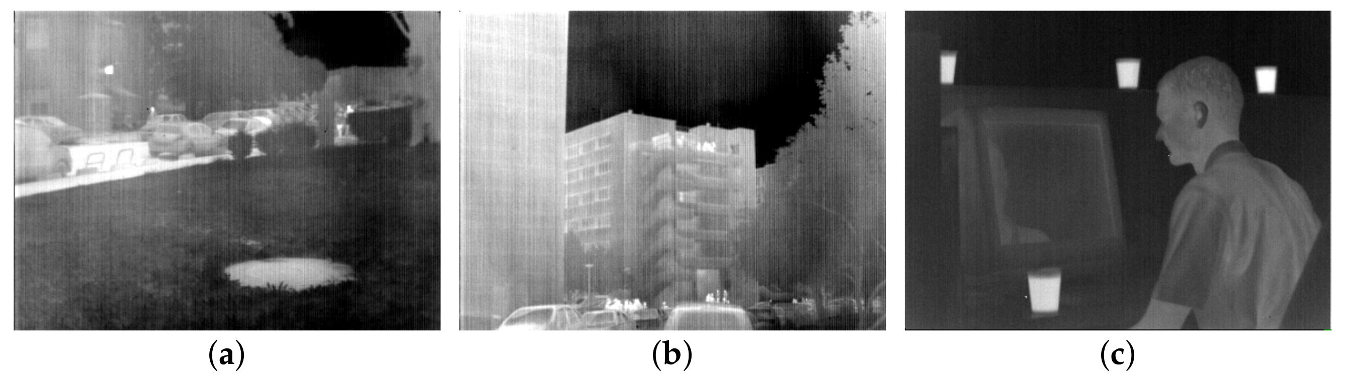
Figure 9.
Destriping results of Experiment 1 for conventional TIR imagery. (a) MIRE; (b) 1D-GF; (c) TwSF; (d) DLSNUC; (e) WDNN; (f) Ours.
Figure 9.
Destriping results of Experiment 1 for conventional TIR imagery. (a) MIRE; (b) 1D-GF; (c) TwSF; (d) DLSNUC; (e) WDNN; (f) Ours.

Figure 10.
Destriping results of Experiment 2 for conventional TIR imagery. (a) MIRE; (b) 1D-GF; (c) TwSF; (d) DLSNUC; (e) WDNN; (f) Ours.
Figure 10.
Destriping results of Experiment 2 for conventional TIR imagery. (a) MIRE; (b) 1D-GF; (c) TwSF; (d) DLSNUC; (e) WDNN; (f) Ours.

Figure 11.
Destriping results of Experiment 3 for conventional TIR imagery. (a) MIRE; (b) 1D-GF; (c) TwSF; (d) DLSNUC; (e) WDNN; (f) Ours.
Figure 11.
Destriping results of Experiment 3 for conventional TIR imagery. (a) MIRE; (b) 1D-GF; (c) TwSF; (d) DLSNUC; (e) WDNN; (f) Ours.

Figure 12.
Comparisons of the pixels in a single row from three sets of experimental results. (a) Pixel values in the 20th row from Experiment 1; (b) Pixel values in the 140th row from Experiment 2; (c) Pixel values in the 50th row from Experiment 3.
Figure 12.
Comparisons of the pixels in a single row from three sets of experimental results. (a) Pixel values in the 20th row from Experiment 1; (b) Pixel values in the 140th row from Experiment 2; (c) Pixel values in the 50th row from Experiment 3.

Figure 13.
Destriping results in the extreme case for conventional TIR imagery. (a) Original image; (b) MIRE; (c) 1D-GF; (d) TwSF; (e) DLSNUC; (f) WDNN; (g) Ours.
Figure 13.
Destriping results in the extreme case for conventional TIR imagery. (a) Original image; (b) MIRE; (c) 1D-GF; (d) TwSF; (e) DLSNUC; (f) WDNN; (g) Ours.

Figure 14.
Remote sensing spectral images used in the three experiments. (a) Experiment 1; (b) Experiment 2; (c) Experiment 3.
Figure 14.
Remote sensing spectral images used in the three experiments. (a) Experiment 1; (b) Experiment 2; (c) Experiment 3.

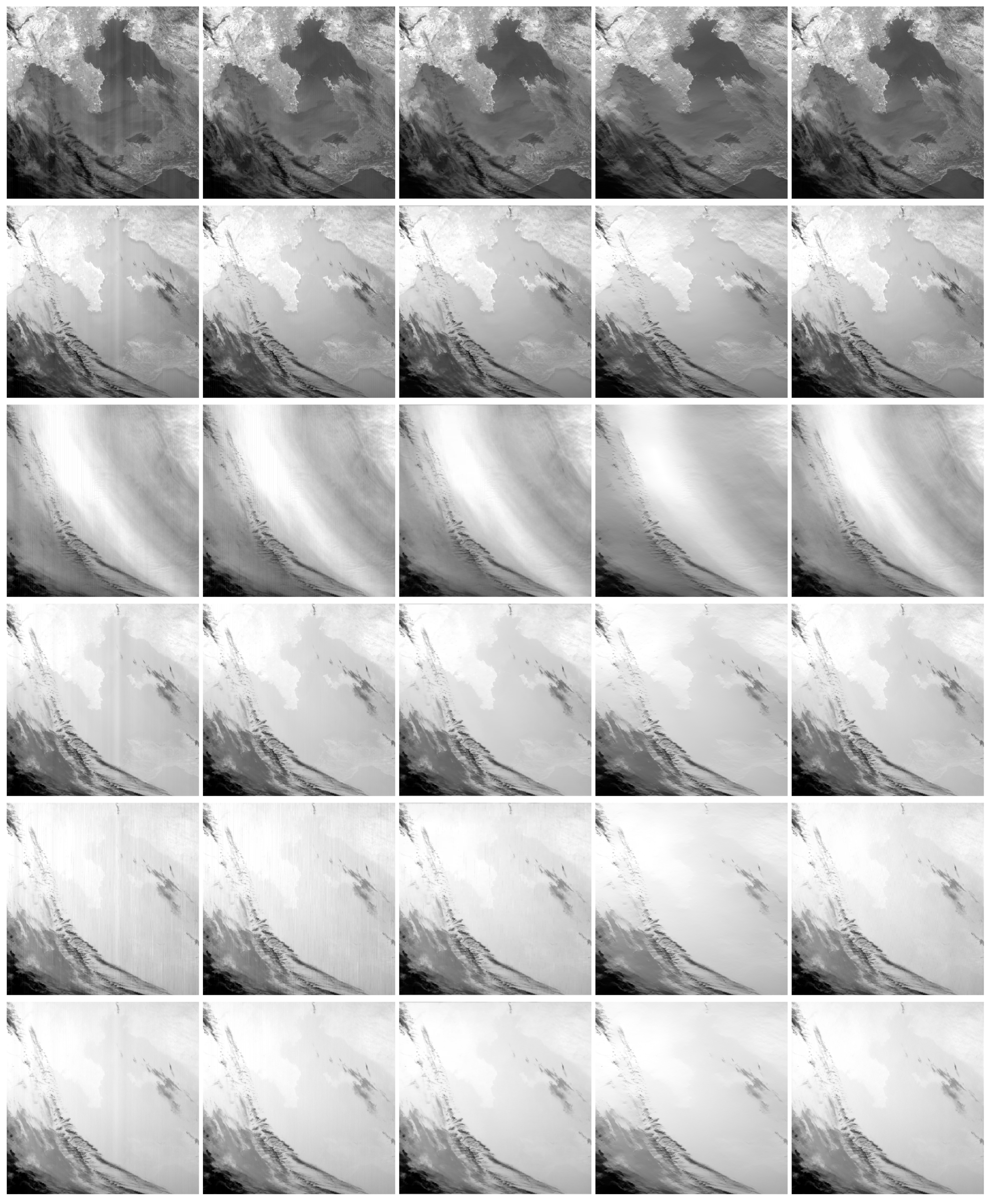
Figure 15.
Desrtiping results of Experiment 1 for remote sensing spectral images. From left to right: WFAF, SLD, RLSID, DSM- and Ours. From top to bottom: Band 21, 24, 27, 33, 34 and 35 from the MOD021KM product. Readers are recommended to zoom in all figures for better observation.
Figure 15.
Desrtiping results of Experiment 1 for remote sensing spectral images. From left to right: WFAF, SLD, RLSID, DSM- and Ours. From top to bottom: Band 21, 24, 27, 33, 34 and 35 from the MOD021KM product. Readers are recommended to zoom in all figures for better observation.

Figure 16.
Desrtiping results of Experiment 2 for remote sensing spectral images. From left to right: WFAF, SLD, RLSID, DSM- and Ours. From top to bottom: Band 21, 24, 27, 33, 34 and 35 from the MOD021KM product. Readers are recommended to zoom in all figures for better observation.
Figure 16.
Desrtiping results of Experiment 2 for remote sensing spectral images. From left to right: WFAF, SLD, RLSID, DSM- and Ours. From top to bottom: Band 21, 24, 27, 33, 34 and 35 from the MOD021KM product. Readers are recommended to zoom in all figures for better observation.

Figure 17.
Desrtiping results of Experiment 3 for remote sensing spectral images. From left to right: Band 27, 34 and 36 from the MOD02SSH product. From top to bottom: WFAF, SLD, LRSID, DSM- and Ours. Readers are recommended to zoom in all figures for better observation.
Figure 17.
Desrtiping results of Experiment 3 for remote sensing spectral images. From left to right: Band 27, 34 and 36 from the MOD02SSH product. From top to bottom: WFAF, SLD, LRSID, DSM- and Ours. Readers are recommended to zoom in all figures for better observation.
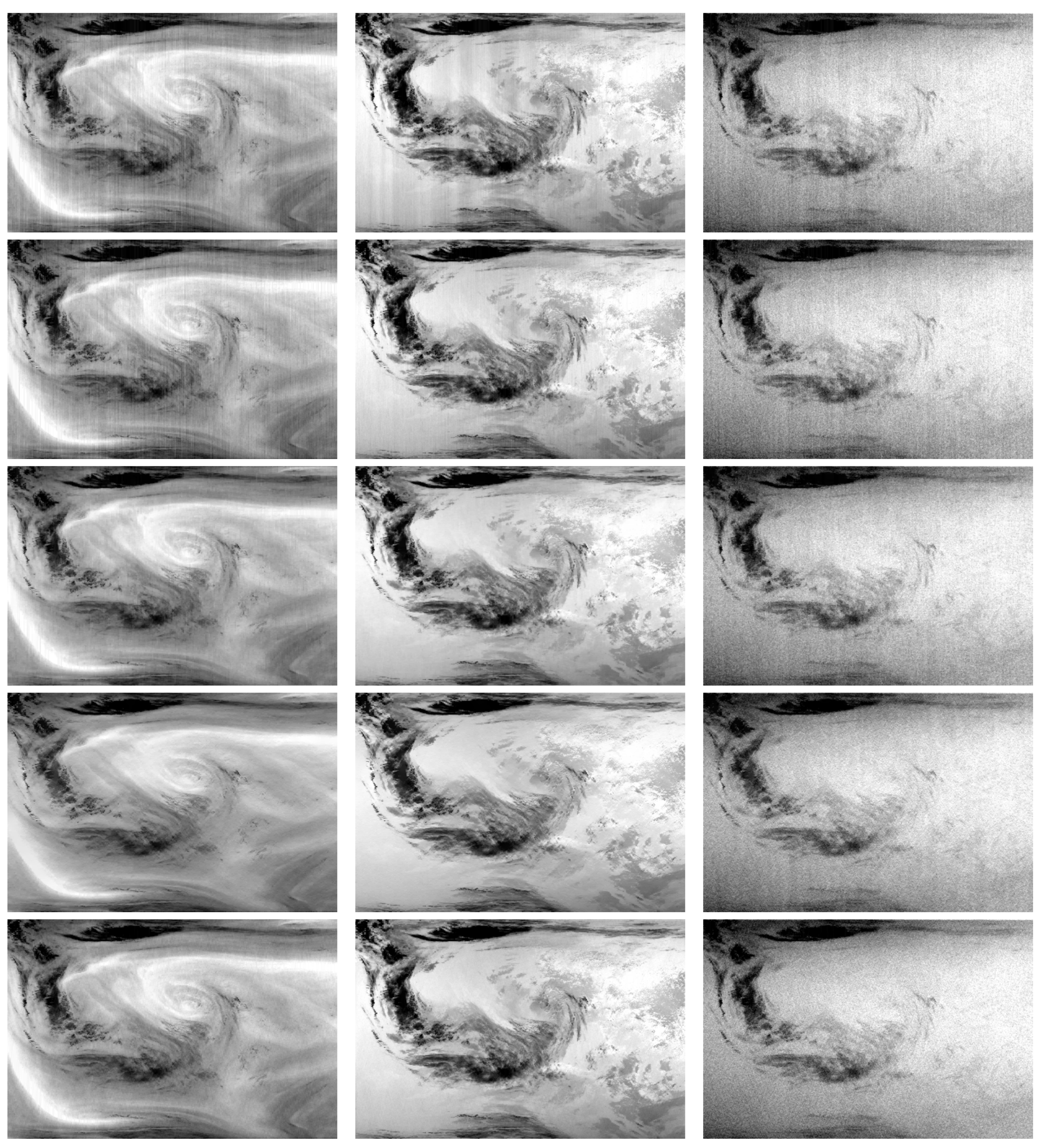
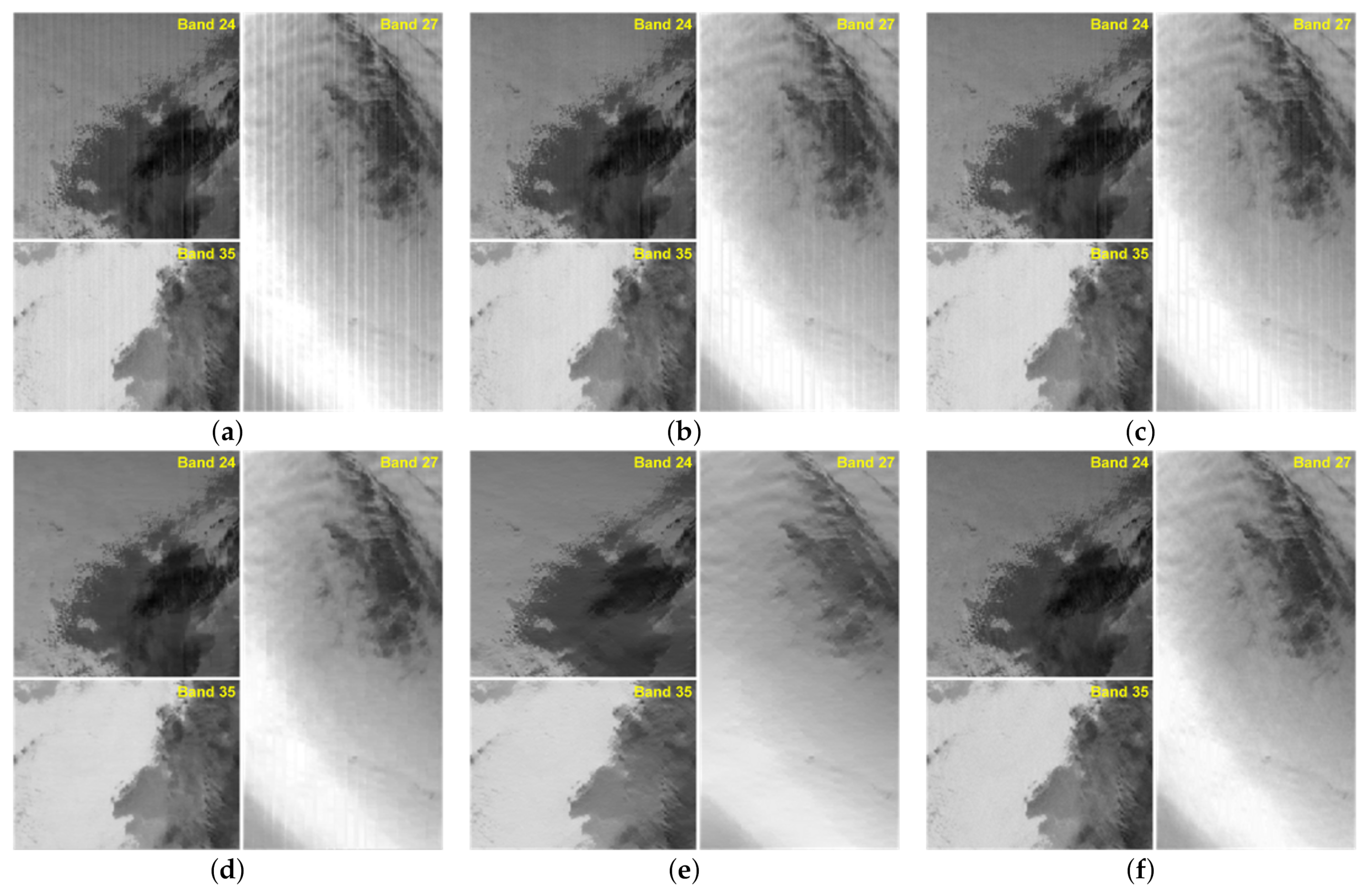
Figure 18.
Visual comparison of partial areas corresponding to Figure 15. (a) Original image parts from Band 24, 27 and 35; (b) WFAF; (c) SLD; (d) LRISD; (e) DSM-; (f) Ours.
Figure 18.
Visual comparison of partial areas corresponding to Figure 15. (a) Original image parts from Band 24, 27 and 35; (b) WFAF; (c) SLD; (d) LRISD; (e) DSM-; (f) Ours.

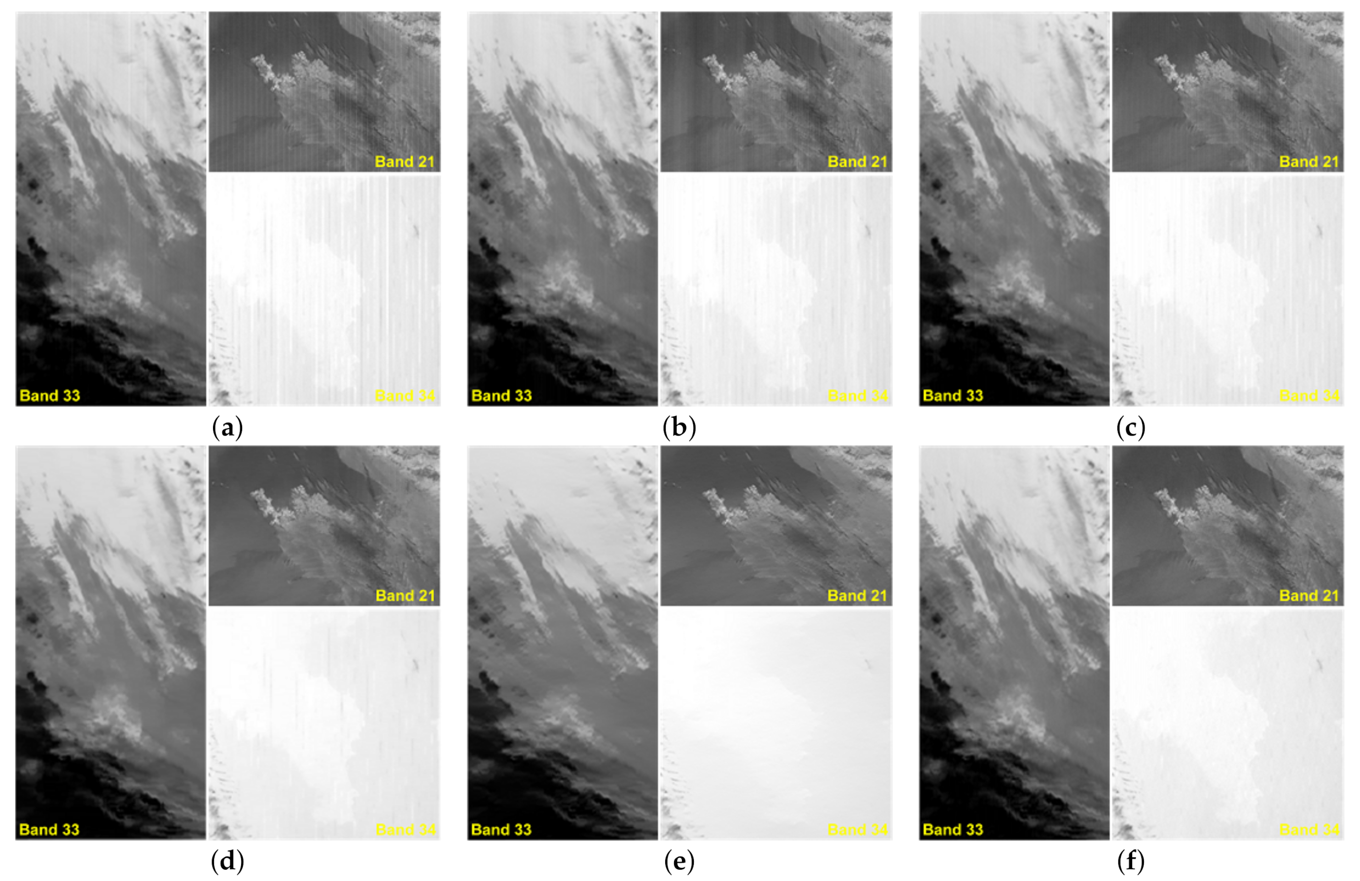
Figure 19.
Visual comparison of partial areas corresponding to Figure 16. (a) Original image parts from Band 21, 33 and 34; (b) WFAF; (c) SLD; (d) LRISD; (e) DSM-; (f) Ours.
Figure 19.
Visual comparison of partial areas corresponding to Figure 16. (a) Original image parts from Band 21, 33 and 34; (b) WFAF; (c) SLD; (d) LRISD; (e) DSM-; (f) Ours.

Figure 20.
Mean cross-track profiles of the Band 21 image from Experiment 1. (a) Original; (b) WFAF; (c) SLD; (d) LRISD; (e) DSM-; (f) Ours.
Figure 20.
Mean cross-track profiles of the Band 21 image from Experiment 1. (a) Original; (b) WFAF; (c) SLD; (d) LRISD; (e) DSM-; (f) Ours.
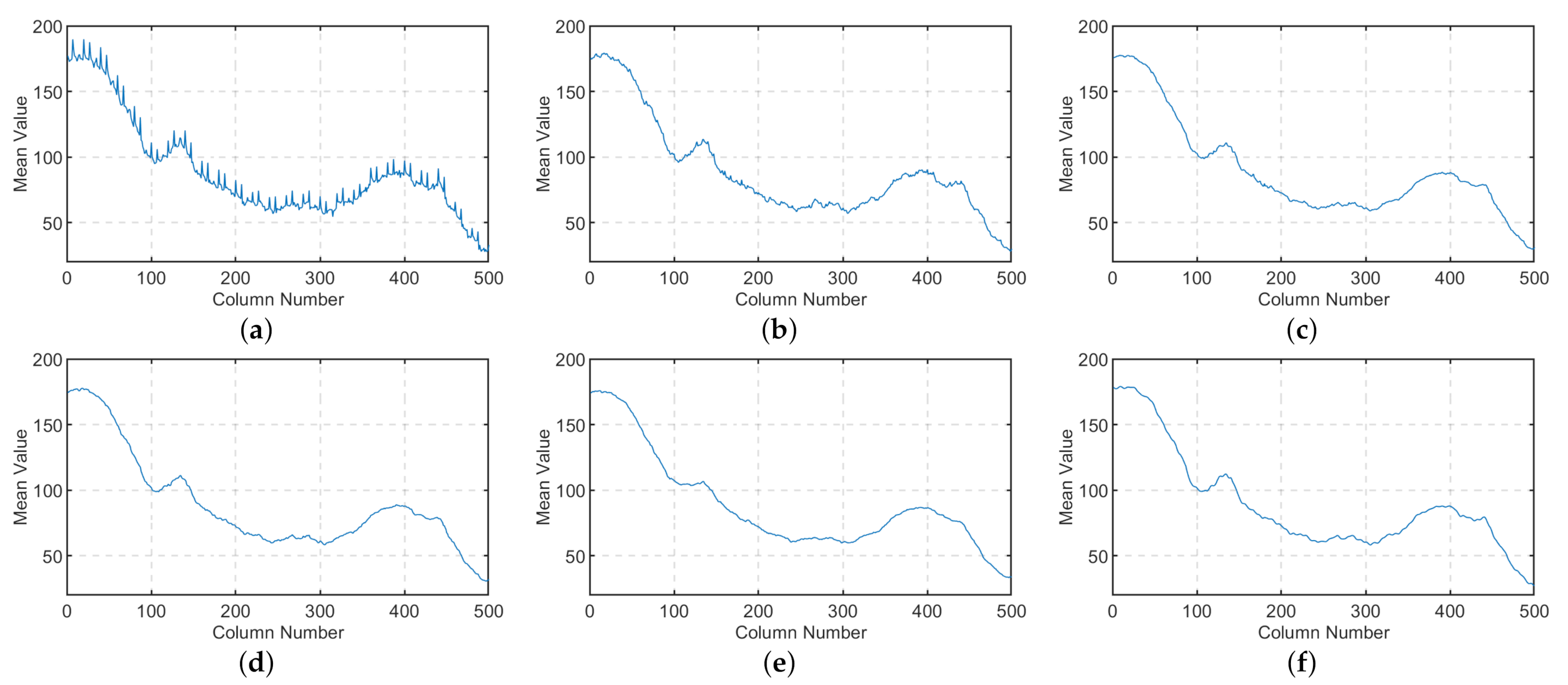
Figure 21.
Mean cross-track profiles of the Band 27 image from Experiment 2. (a) Original; (b) WFAF; (c) SLD; (d) LRISD; (e) DSM-; (f) Ours.
Figure 21.
Mean cross-track profiles of the Band 27 image from Experiment 2. (a) Original; (b) WFAF; (c) SLD; (d) LRISD; (e) DSM-; (f) Ours.

Figure 22.
Mean row power spectrums of the Band 21 image from Experiment 2. (a) Original; (b) WFAF; (c) SLD; (d) LRISD; (e) DSM-; (f) Ours.
Figure 22.
Mean row power spectrums of the Band 21 image from Experiment 2. (a) Original; (b) WFAF; (c) SLD; (d) LRISD; (e) DSM-; (f) Ours.

Figure 23.
Mean row power spectrums of the Band 27 image from Experiment 2. (a) Original; (b) WFAF; (c) SLD; (d) LRISD; (e) DSM-; (f) Ours.
Figure 23.
Mean row power spectrums of the Band 27 image from Experiment 2. (a) Original; (b) WFAF; (c) SLD; (d) LRISD; (e) DSM-; (f) Ours.

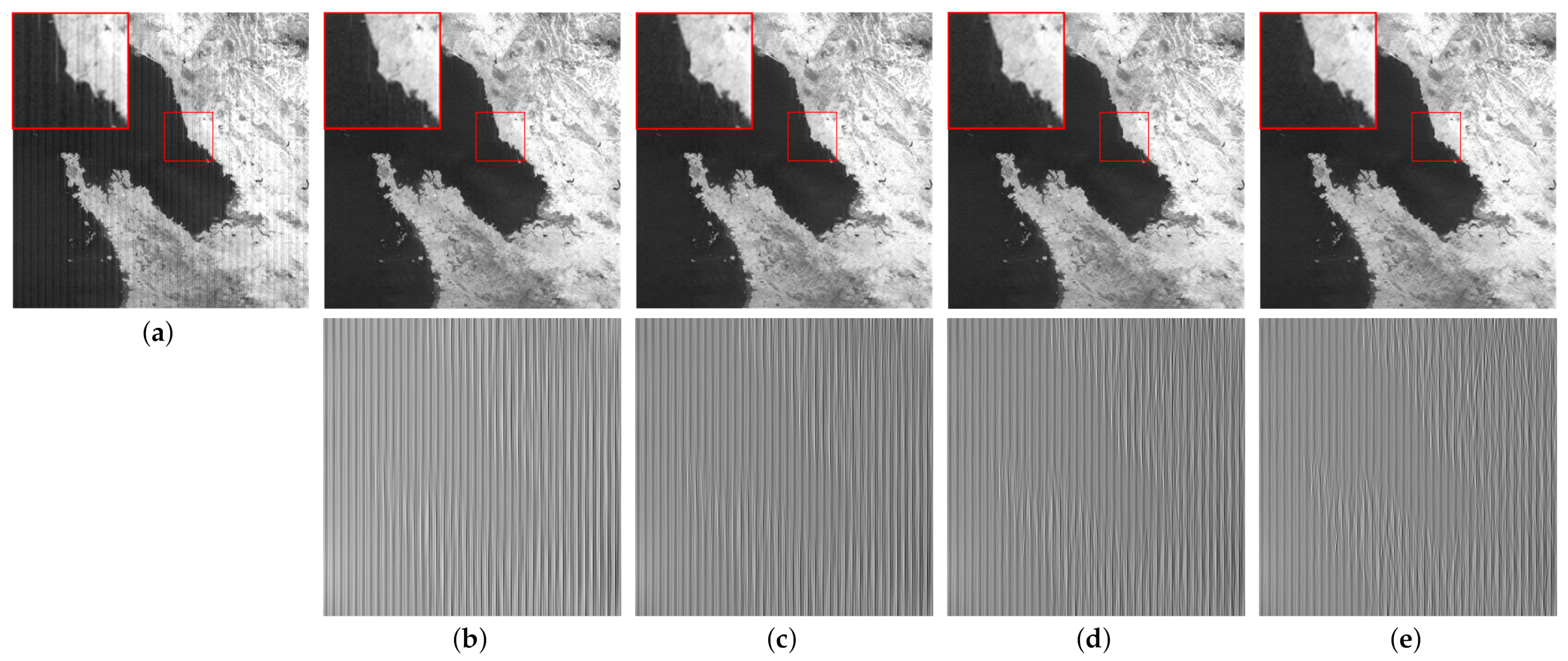
Figure 24.
The influence of the parameter on the destriping performance. (a) Original image; (b) Result with ; (c) Result with ; (d) Result with ; (e) Result with .
Figure 24.
The influence of the parameter on the destriping performance. (a) Original image; (b) Result with ; (c) Result with ; (d) Result with ; (e) Result with .

Table 1.
Quantitative evaluation results of three experiments for conventional TIR images.
| Method | Experiment 1 | Experiment 2 | Experiment 3 | |||||||||
|---|---|---|---|---|---|---|---|---|---|---|---|---|
| Q | RMSE | Q | RMSE | Q | RMSE | |||||||
| MIRE | 0.138 | 0.160 | 9.82 | 0.0217 | 0.125 | 0.328 | 8.66 | 0.0286 | 0.177 | −0.470 | 17.08 | 0.0059 |
| 1D-GF | 0.131 | 0.139 | 9.11 | 0.0209 | 0.120 | 0.223 | 7.83 | 0.0282 | 0.164 | −0.284 | 11.89 | 0.0068 |
| TwSF | 0.131 | 0.149 | 9.09 | 0.0231 | 0.119 | 0.235 | 7.81 | 0.0318 | 0.166 | −0.382 | 12.46 | 0.0056 |
| DLSNUC | 0.100 | 0.499 | 11.05 | 0.0220 | 0.088 | 0.567 | 10.71 | 0.0292 | 0.126 | 0.255 | 18.07 | 0.0057 |
| WDNN | 0.129 | 0.256 | 9.34 | 0.0207 | 0.118 | 0.421 | 8.55 | 0.0281 | 0.166 | −0.021 | 15.70 | 0.0047 |
| Ours | 0.126 | 0.526 | 11.47 | 0.0200 | 0.114 | 0.618 | 11.36 | 0.0271 | 0.162 | 0.283 | 19.32 | 0.0042 |
Table 2.
Quantitative evaluation of destriping methods on remote sensing spectral images.
| Image | Index | Original | WFAF | SLD | LRSID | DSM- | Ours |
|---|---|---|---|---|---|---|---|
| Band 21 | ICV1 | 21.8910 | 28.0554 | 28.0749 | 31.8895 | 36.5370 | 31.4056 |
| ICV2 | 18.5833 | 19.6632 | 21.8711 | 24.0064 | 29.5712 | 24.6683 | |
| MRD1 | - | 0.0167 | 0.0182 | 0.0253 | 0.0376 | 0.0248 | |
| MRD2 | - | 0.0131 | 0.0139 | 0.0157 | 0.0320 | 0.0135 | |
| Band 24 | ICV1 | 3.8014 | 3.8561 | 3.8729 | 3.9096 | 4.4591 | 4.1827 |
| ICV2 | 87.8540 | 122.4623 | 125.2533 | 151.5480 | 154.6837 | 149.2865 | |
| MRD1 | - | 0.0224 | 0.0268 | 0.0350 | 0.0980 | 0.0333 | |
| MRD2 | - | 0.0106 | 0.0087 | 0.0110 | 0.0212 | 0.0101 | |
| Band 27 | ICV1 | 14.5392 | 17.2013 | 16.5835 | 17.8278 | 27.7905 | 18.5027 |
| ICV2 | 38.7568 | 54.0097 | 54.5366 | 65.7343 | 125.2244 | 73.0345 | |
| MRD1 | - | 0.0204 | 0.0211 | 0.0286 | 0.0356 | 0.0258 | |
| MRD2 | - | 0.0259 | 0.0302 | 0.0402 | 0.0544 | 0.0372 | |
| Band 33 | ICV1 | 5.5825 | 5.4789 | 5.5875 | 5.7910 | 8.7910 | 5.6949 |
| ICV2 | 108.4053 | 164.1888 | 166.2775 | 231.5580 | 253.2472 | 212.7835 | |
| MRD1 | - | 0.0102 | 0.0067 | 0.0136 | 0.0169 | 0.0124 | |
| MRD2 | - | 0.0044 | 0.0034 | 0.0074 | 0.0115 | 0.0065 | |
| Band 34 | ICV1 | 14.4918 | 15.4177 | 15.7350 | 15.9210 | 18.2459 | 16.3604 |
| ICV2 | 40.4405 | 54.1095 | 58.4728 | 77.3437 | 127.7196 | 90.1767 | |
| MRD1 | - | 0.0319 | 0.0482 | 0.0651 | 0.1450 | 0.0585 | |
| MRD2 | - | 0.0102 | 0.0110 | 0.0131 | 0.0147 | 0.0126 | |
| Band 35 | ICV1 | 7.8907 | 8.2272 | 8.3232 | 9.5049 | 13.2531 | 10.3291 |
| ICV2 | 60.8430 | 70.1713 | 75.3580 | 92.3648 | 153.1217 | 92.1730 | |
| MRD1 | - | 0.0115 | 0.0151 | 0.0289 | 0.0344 | 0.0252 | |
| MRD2 | - | 0.0084 | 0.0099 | 0.0179 | 0.0414 | 0.0175 | |
| SAM1 | - | 0.0261 | 0.0218 | 0.0293 | 0.0533 | 0.0214 | |
| SAM2 | - | 0.0149 | 0.0124 | 0.0143 | 0.0178 | 0.0121 |
Table 3.
Average running time (s) of different methods for conventional TIR images with size 288 × 384 and remote sensing spectral images with size 500 × 500.
Table 3.
Average running time (s) of different methods for conventional TIR images with size 288 × 384 and remote sensing spectral images with size 500 × 500.
| Image Size | MIRE | 1D-GF | TwSF | DLSNUC | Ours | Image Size | WFAF | SLD | LRSID | DSM- | Ours |
|---|---|---|---|---|---|---|---|---|---|---|---|
| 288 × 384 | 0.07 | 0.06 | 0.01 | 0.46 | 0.38 | 500 × 500 | 0.25 | 0.04 | 16.37 | 34.52 | 1.06 |
Publisher’s Note: MDPI stays neutral with regard to jurisdictional claims in published maps and institutional affiliations. |
© 2020 by the authors. Licensee MDPI, Basel, Switzerland. This article is an open access article distributed under the terms and conditions of the Creative Commons Attribution (CC BY) license (http://creativecommons.org/licenses/by/4.0/).
Share and Cite
MDPI and ACS Style
Zeng, Q.; Qin, H.; Yan, X.; Yang, T. Fourier Domain Anomaly Detection and Spectral Fusion for Stripe Noise Removal of TIR Imagery. Remote Sens. 2020, 12, 3714. https://0-doi-org.brum.beds.ac.uk/10.3390/rs12223714
AMA Style
Zeng Q, Qin H, Yan X, Yang T. Fourier Domain Anomaly Detection and Spectral Fusion for Stripe Noise Removal of TIR Imagery. Remote Sensing. 2020; 12(22):3714. https://0-doi-org.brum.beds.ac.uk/10.3390/rs12223714
Chicago/Turabian StyleZeng, Qingjie, Hanlin Qin, Xiang Yan, and Tingwu Yang. 2020. "Fourier Domain Anomaly Detection and Spectral Fusion for Stripe Noise Removal of TIR Imagery" Remote Sensing 12, no. 22: 3714. https://0-doi-org.brum.beds.ac.uk/10.3390/rs12223714
Note that from the first issue of 2016, this journal uses article numbers instead of page numbers. See further details here.