Bringing Bathymetry LiDAR to Coastal Zone Assessment: A Case Study in the Southern Baltic


1
Faculty of Civil and Environmental Engineering, Gdansk University of Technology, Gabriela Narutowicza 11/12, 80-233 Gdansk, Poland
2
Apeks Company Ltd. Jaskowa Dolina 81, 80-286 Gdansk, Poland
Remote Sens. 2020, 12(22), 3740; https://0-doi-org.brum.beds.ac.uk/10.3390/rs12223740
Submission received: 14 September 2020
/
Revised: 3 November 2020
/
Accepted: 12 November 2020
/
Published: 13 November 2020
(This article belongs to the Special Issue Remote Sensing of Coastal Processes)
Abstract
:One of the major tasks in environmental protection is monitoring the coast for negative impacts due to climate change and anthropopressure. Remote sensing techniques are often used in studies of impact assessment. Topographic and bathymetric procedures are treated as separate measurement methods, while methods that combine coastal zone analysis with underwater impacts are rarely used in geotechnical analyses. This study presents an assessment of the bathymetry airborne system used for coastal monitoring, taking into account environmental conditions and providing a comparison with other monitoring methods. The tests were carried out on a section of the Baltic Sea where, despite successful monitoring, coastal degradation continues. This technology is able to determine the threat of coastal cliff erosion (based on the geotechnical analyses). Shallow depths have been reported to be a challenge for bathymetric Light Detection and Ranging (LiDAR), due to the difficulty in separating surface, water column and bottom reflections from each other. This challenge was overcome by describing the classification method used which was the CANUPO classification method as the most suitable for the point cloud processing. This study presents an innovative approach to identifying natural hazards, by combining analyses of coastal features with underwater factors. The main goal of this manuscript is to assess the suitability of using bathymetry scanning in the Baltic Sea to determine the factors causing coastal erosion. Furthermore, a geotechnical analysis was conducted, taking into account geometrical ground change underwater. This is the first study which uses a coastal monitoring approach, combining geotechnical computations with remote sensing data. This interdisciplinary scientific research can increase the awareness of the environmental processes.
1. Introduction
Global average temperatures are gradually increasing: this has far-reaching social and environmental consequences [1,2,3]. Mitigating the adverse impacts of climate change can reduce the global financial and social risks it poses. Coherent and forward-thinking adaptation strategies have the potential to stimulate sustainable regional development, while improving the quality of everyday life. The European Union Strategy for the Baltic Sea [4] outlines three priority tasks: protecting the aquatic environment, connecting the region, and increasing prosperity. Utilisation of appropriate research tools, as well as cooperation between local authorities, businesses and academia can actively support climate change mitigation and adaptation.
Threats to the coastline and coastal ecosystems can arise from both natural and anthropogenic sources: climate change amplifies natural processes, for example, the extent of dune sections that are in recession by erosion, abrasion or deflation has increased [5,6,7]. Natural or man-made deflation can cause dunes to move inland, forming low spits, which increase the possibility of flooding. Moreover, it changes the ecosystem, thus causing problems for flora and fauna. In the last century, the anthropogenic footprint on coastal ecosystems has intensified.
This study presents the results of coastal zone measurements by airborne bathymetry technology, focussing on the factors that affect coastal stability. A more comprehensive assessment requires the registration of endangered areas to consider coastal zones both on land and underwater. The study provides reliable, previously unavailable, laser data on the complicated geomorphology of the southern Baltic. This research discusses the pros and cons of using Airborne Bathymetry Light Detection and Ranging (LiDAR) technology (ALB) in the Baltic Sea, with a view to encouraging integrated, multidisciplinary research in coastline monitoring and protection. The area studied in this experiment shows that the protection of the seashore against erosion is ineffective. Changes to the coastline have taken place in an uncontrolled manner, and safeguards against the natural erosion of the shores have not been able to stop the destructive impact of the sea. The lack of coherent action by state and local government bodies has not been conducive to shaping the proper protection within the technical belt along the shoreline. A serious and unsolved problem has been caused by the clash between economic goals aimed at developing tourist infrastructure, and natural goals related to the protection of the natural environment.
To date, the relevant literature on coastal cliffs’ failure (e.g., rockfall, erosion) has not considered the geometrical change of cliffs under water [8,9,10,11,12]. Integration of data from the LiDAR systems for topographic evaluation enables the determination of an appropriate geotechnical model [13], but only considers terrestrial parts of the coast. Given their irregular topography, cliffs and shorelines are difficult to integrate correctly as a numerical model. The knowledge of remote sensing techniques has allowed the development of numerical models of the coast; however, the utilisation of topographic and bathymetric relief studies has not been observed [14,15,16]. A comprehensive, rapid analysis of at-risk locations is fundamental for creating a warning system for where the degradation is occurring; however, this remains a challenge.
Previous studies have determined the water visibility conditions, under which the ALB system can successfully take measurements, taking into account the conditions in an area under threat from coastal erosion [17,18,19,20]. This study aims to characterise the conditions for performing measurements, together with defining the time scale for these methodologies.
Many studies have explored commonly used methods of sea bottom measurement, and identified their application in shallow water mapping and analysing the effects of coastal changes. The advantages and disadvantages of these measurement techniques are considered below.
Topographic–bathymetric maps can be used for coastal management, economic activity in coastal areas and providing safety guidelines for users of the natural environment and coastal infrastructure [21]. For example, appropriate terrain models can help identify accessible and profitable fishing locations for local anglers, and determine the tendency for changes in these areas [21]. The most important aspect of topographic–bathymetric monitoring is its ability to determine flood hazards that could negatively affect coastal infrastructure [22] and the natural environment [23,24,25]. Furthermore, bathymetry measurements can constantly check calculations or determine the tendency of degradation in research areas [26].
Multibeam sensors are the most commonly used sensors for measuring depth and developing digital models of the sea bottom [27,28,29,30]. The proposed method for using multibeam sensor analyses is to use algorithms to facilitate data collection and processing, and then to test them empirically. These solutions, however, are time-consuming and suboptimal for determining the tendency of changes in short-term temporal models: covering an area of several square kilometres can take up to several days.
Satellite products are used to create calibration models for calculations [31,32]. Previous studies have used satellite products to determine water depth [33], compare different measurement methods [34], and to investigate trends of change [35,36]; however, compared with ALB data, the lower level of detail provided by this information excludes the possibility of analysing local phenomena [13,37]. Despite these limitations, examining the trends of change in large areas through satellite products is better than using airborne techniques, due to the size and quality of the data [38,39].
There are several reasons why ALB technology is not widely used among geomorphologists. It is very expensive as it requires a plane to mount the device to. A number of environmental factors, moreover, such as water clarity, vegetation and surface waves influence the transmission of the laser pulse through water, thus affecting the strength and shape of the return pulse [40]. To mitigate these disturbances, it is important to first define the environmental conditions in the water body of interest. Shallow depths have also been reported to be a challenge for bathymetric LiDAR due to the difficulty in separating the water surface, column and bottom reflections [41,42,43,44]. Researchers have sought to address data quality concerns [45,46,47], resulting in different levels of accuracy between topographic and bathymetric results. These results are significantly better than those obtained by satellite techniques, however, the measurement time (using unmanned aerial vehicles) and the spatial coverage are suboptimal for larger areas. In the subsequent data analysis, resolution differences have to be taken into consideration.
Airborne measurement systems can be used to develop topographic–bathymetric maps, as evidenced by the LiDAR topographic, multispectral images and other available data libraries [47]. Taramelli et al. (2020) postulated that when the resolution increases, the cost of measurement increases in a linear fashion [47]. Considering the differences between data from photos and laser scanners [48], they can be used in conjunction to determine the appropriate boundary conditions for the obtained data resolutions. Agrafiotis et al. [49] and Bue et al. [50] have put forward solutions for photographic conditions, while Mandlberger et al. [51] has determined the conditions for the scanner.
This study discusses the suitability of using a bathymetric scanner for coastal monitoring on the southern Baltic coast. To the author’s knowledge, this study is the first to introduce the geotechnical application of bathymetric scanning in these waters. The results obtained from using airborne systems are intended for a wide range of recipients, ranging from governments and local authorities responsible for coastal management and protection, to investors planning waterfront developments. To consider the practical application of this method, the aims of this study are as follows:
- -
- data collection and processing;
- -
- digital Terrain Model (DTM) creation for geometric changes analysis;
- -
- obtaining reliable bathymetric data for shallow water areas where geotechnical analysis can be conducted.
2. Materials and Methods
2.1. Baltic Sea Region
The Baltic Sea is one of the most polluted in the world. Due to the unique conditions of this area (low salinity, poor water exchange, multiple river mouths), ALB technology has not previously been utilised to measure coastal erosion. The Baltic Sea is linked to the North Sea by a series of narrow passages through the Danish straits [52]. This area is therefore subject to local atmospheric phenomena: air movement is a more significant factor than currents in the circulation of water [53]. The location and strength of the jet stream determine the weather: in winter, the central or western jet streams particularly affect the southern Baltic, resulting in warmer temperatures. In the summer, the impact of the subtropical high-pressure system increases and expands north [53]. The Baltic Sea is therefore an important area to study climate change, and it is necessary to develop a methodology to assess the impact of global warming. In addition, the sandy southern Baltic coast undergoes greater changes than the rocky northern coast, due to its geological structure and climatic conditions. Intense erosion has occurred on the open coastline of the southern Baltic in the past century. Research has linked these conditions to the size of storms that occur in the Baltic Sea and the rising water level that accompanies these hazardous conditions [54,55,56,57].
These studies have also noted that a drastic increase in serious disturbances, caused by global climate change, are expected until 2100. Extreme levels of Baltic Sea waters are frequently observed in autumn and winter. Thus, ecosystem deterioration is anticipated to continue. The analysis of environmental changes related to the degradation of the natural environment will allow for the assessment of this phenomenon. Achieving correct conclusions will be associated with correctly performed measurements. The possibilities for measuring and analysing the results are described in this manuscript.
Taking the local environmental conditions into consideration, the most important factors will be the measurements carried out in spring and autumn, due to the marine climate (Cfb—Köppen climate classification [58]) of the southern Baltic sea. In this period the greatest number of extreme weather conditions (i.e., storms) are observed. In this study, four parameters were utilised for the assessment of conditions to ensure adequate measurement: water turbidity, wave height, cloudiness, and level of sunlight when taking pictures. Each of these measurements was evaluated on a five-point scale at each location, with one representing unacceptable conditions, up to five for ideal conditions.
2.2. Study Area
The study location was based on measurements prepared by the Institute of Meteorology and Water Management for the Polish Ministry of the Environment [59]. The study area is characterised by the presence of glacial plateaus, interspersed with a number of valley formations, which have their origins in former ice-marginal valleys from the Vistula glaciation phase [59]. The behaviour of the coast has been monitored and analysed for the past few decades, and significant degradation has been observed as a result of abrasion and groundwater conditions. The exact sampling locations are shown in Figure 1.
The existing protection, in the form of a gabion structure and slope protection, have not proven to be successful in the long-term and they have not improved the stability of the cliff slopes. The studies conducted so far have not been sufficient in determining the factors threatening the shore [11,12,13].
2.3. Measurements
The measurement campaign was divided into several stages which provides a concise, step-by-step account of the research procedure:
- Establishment of a control points network, in accordance with the applicable law. As a rule, the points should be evenly distributed over the entire measured area, treating some of them as reference points, some of them as control points. Their accuracy should be greater than that of the ALB measurement.
- Photogrammetric flights using ALB technology with simultaneous manual depth measurements (the accuracy of manual depth measurements should be even or greater than that of the ALB measurement). The acquisition should performed under appropriate weather conditions (which are described below).
- Processing of data, in terms of checking their utility in the assessment of coastal erosion. This processing consists of: classifying the ground class from the point cloud, analysis of the geometrical correctness of the measurement in relation to other methods, as well as developing a 3D model and geometrically comparing its changes with respect to successive flights over time.
- Geotechnical studies based on Factor of Safety assessment of each Ground Layer to see in what circumstances the coast’s loss of stability may occur. The details of the calculations are discussed in Section 2.6.3.
The measurement of control and reference points, which were the same for each of the flights, was done using the Real Time Kinematic (RTK) Global Navigation Satellite System (GNSS) technique and a Terrestrial Laser Scanner (TLS), following the methods previously described in [13]. Locally, at each of the TLS locations, the measured coordinates were compared with those acquired for stabilised points (Figure 2a) and the precision was compared to the DTM with known accuracy and precision. Efforts were made to locally distribute points to control the resolution of the data obtained. In several selected locations throughout the area, perpendicular to the coastline, manual sea bottom measurements were made using the RTK GNSS method (Figure 2b), and then cross-sections were compared to the point cloud obtained from ALB. To supplement the four-step methodology described above, an extensive analysis was undertaken for each step that led to the specification of weather conditions that had significant impacts on obtaining reliable bathymetry information.
Figure 3 illustrates how the southern Baltic Sea changes, in relation to the prevailing weather conditions, over the five-point scale. Figure 3a shows the conditions designated as 1–2; nearly full cloud cover is observed, preventing photogrammetric flights, and large waves with visible half-breaks and high water silting restrict water penetration by the laser beam. In such conditions (or worse), topographic–bathymetric measurements are not possible. During the fieldwork, the weather changed unfavourably during manual measurements. Manually measured points were compared with the results of the point cloud, but were not taken into account in the final report. Figure 3b shows the conditions of scales 2–3, where appropriate atmospheric conditions are observed, allowing for the topography of the terrain to be recorded. However, the increased sea level and high silting make it impossible to perform correct ALB measurements. In the conditions assessed as scales 3–4, as shown in Figure 3c, the appropriate weather conditions enable the photogrammetric mission to be completed, with a calm sea and a visible bottom at the shore being observed. Some silting of the reservoir can be observed, which may cause erroneous measurement results. The additional analysis (defined as an assessment of the recorded suspensions density in water) of the point cloud data showed that, despite the calm sea and good weather conditions, it was necessary to wait a few days for the suspensions floating in the water to naturally sink to the bottom. This will result in better classification results, thus achieve better depth measurements. Under the right conditions, which is quite rare in the southern Baltic Sea, the effect shown in Figure 3d can be obtained (scale 4–5), where the bottom is visible at a large distance from the shore. Depending on the weather conditions, the difference in depth ranged from 0 m (Figure 3b) to 15 m (Figure 3d), using a 1-secchi depth scanner. However, even under such conditions, the measurement may not be successful due to the amount of algae lying on the bottom of the shore. This may cause issues with the penetration of the scanner beam, thus a completely dense cloud of points may not be obtained. In places where, despite very good conditions for measurements some obstacles (algae, rocky materials, anthropogenic waste) may appear, it is recommended to manually measure the bottom bathymetry.
2.4. Platforms and Systems Used
For the experiment, Riegl VQ820G (Manufacturer: Riegl GmBH, Austria) and Riegl VQ-1560i-DW (Manufacturer: Riegl GmBH, Austria) systems were used. The following companies carried out the measurements: Opegieka (HQ: Elblag, Poland) and AirborneHydroMapping (HQ: Innsbruck, Austria). For accurate methodology, the data were pre-processed according to the manufacturer’s software, then exported in a known extension. The technical aspects of the data acquired for each of the devices are given in Table 1, including the weather conditions (five-point scale) and the final point cloud count.
Additional measurements shown in Table 1 include red laser scanning and aerial photographs of the entire study area. These additional datasets were acquired simultaneously, for measurements with an ALB. Individual photos, confirming the atmospheric conditions and terrain models from other periods (comparing objects unchanged in time) were included to verify the results and identify the differences between the measurements.
There are three stages necessary for proper utilisation of the ALB system in the southern Baltic. First, it is very important to obtain data from sea level indicators [60]. Second, the action should be applied, according to obtain good weather conditions [61]: the required sea level should not be exceeded. The experiment shows that it should not exceed 1 m above the average sea level. According to the results of Wolski and Wisniewski [56] and Gierjatowicz et al. [57], sea level exceeding 1 m is associated with high siltation and intensification of difficult environmental conditions (e.g., rainfall). Third, the following conditions should be observed: low winds, weakening sea currents, absence of precipitation, and moderate temperatures. The climate of the southern Baltic Sea very rarely gives rise to ideal conditions (sometimes only several days per year); therefore, it is essential that the equipment used is appropriate for the conditions.
The Riegl VQ-820G laser scanner has the ability to register the bottom up to a Secchi depth of one. However, it is very important that the scanning depth is equal to or above the Secchi depth, to ensure proper registration, regardless of the meteorological and hydrological conditions. After many tests, the CANUPO classification system (the plugin creation has been financed by Université Européenne de Bretagne and The French National Centre for Scientific Research) was selected, due to its reproducibility. This system uses the CloudCompare software (https://www.danielgm.net/cc/), which uses a set of approximately 12,000 points to classify the proper bottom, at a sufficient certainty level. The CANUPO classification algorithm classified laser point datasets using multi-scale measures of the point cloud dimensionalities around each point, the point cloud geometry at a given location and given scales. Class separability, spatial resolution, and the probabilistic confidence of the classification for each point at each scan location were then calculated [62]. The algorithm selects the best combination of scales and a local dimensionality (line, plane, or volume) which gives the greatest separability between classes. Both a balanced accuracy (ba) and Fisher discriminant ratio (fdr) were used to assess the classification results. A high ba value (in a range of 0-1) indicates a good recognition rate of a classifier on a given dataset. A large fdr value implies a good separation between classes [62]. The detailed classification parameters are described in Table 2.
Based on these results, an additional measurement with a RIEGL VQ-1560i-DW laser scanner was performed. This allowed for the registration from the bottom to a Secchi depth of 0.7, with direct registration of two scanner beam lengths (red and green). This type of device was used because it is cheaper to operate and the results between the red and green scanner can be compared with each other. For the geotechnical investigations, efforts were made to obtain the best geometric shape of the studied coast, based on a point cloud that represents the class of ground after classification processing. For this purpose, a cross-section was created in the place where geotechnical data were available. There is no specific depth that should be scanned for geotechnical analysis; therefore, to determine the susceptibility of the soil in geotechnical terms, the best possible result was sought while maintaining the largest possible savings by comparing bathymetry scanning to cheaper methods (e.g., from aerial photographs). Aerial photographs can be used to identify bottom coordinates, as described in [49]. As a comparison, data were acquired through aerial photography, using the methodology described in [63,64].
The use of various methods and systems was motivated by obtaining the most reliable results, in order to better estimate the costs, relative to the value of the obtained geotechnical analyses. Based on previous studies, both systems (laser and photogrammetric) should be able to register a depth of 1 m. Therefore, the question remains as to how it looks at greater depths. Theoretically, the use of an ALB should provide better results than photos due to the cost of carrying out the measurements (it depends on the cost and purpose of the systems). In terms of fieldwork, these methods were identical for measurement acquisition; however, they differ significantly in terms of post-processing. By definition, the point cloud, with a registered bottom, is referenced in a metric system, while with photos it is mandatory to perform manual measurements to calibrate the point model, and post-processing to eliminate noise that interferes with the correct registration of the bottom [49,61,62]. The aerial photos were processed in TerraPhoto software (Terrasolid Ltd. Helsinki, Finland) and AgisoftMetashape software (Agisoft LLC, St. Petersburg, Russia). The first step of processing photosets was extracting all the orientation parameters, then the depth for each camera position was calibrated, creating a dense cloud. By moving the point cloud to the external CloudCompare software, the subsample to a uniform point spacing was performed. To extract the minimum elevation from each cell, the minimum elevation filter was used, thereby reducing the data density and decreasing the influence of surface noise. Calibration and the correctness of the obtained data were checked with manually measured cross sections all along the coast.
Table 3 presents the details of the systems used: all three could be used as separate measurement methods, however, it is important that the user is aware of their specific limitations. For example, one method might complement another, or a method might not be suitable for use in specific environmental conditions found in the southern Baltic. A very important aspect is to define the limitations of these systems. Typically, in photogrammetric missions the point cloud density, the shape of the measurement lines, and the coverage between the stripes are clearly stated. The experiments conducted in this study show that when using a bathymetric scanner under water, none of these parameters are crucial. Firstly, the point density can vary greatly during the filtration and classification processes. Secondly, coverage depends on the topography of the area, and thirdly, the measurement lines are irrelevant to planning. As a result, a noisy digital image is received in every measurement scenario underwater. Therefore, it is important to collect materials which enable the interpretation of the proper bottom correctly, e.g., manual measurements or aerial photographs. The most important factors, however, include weather, local environmental conditions and the Secchi depth to which the device is able to measure. The factors shown in Table 3 provide an overview of the type of data obtained.
2.5. Data Validation
The point clouds were provided by external companies, therefore their accuracy could only be assessed by indirect methods. The appropriate DTMs, from the Centre for Geodetic and Cartographic Documentation in Poland and point clouds acquired from TLS were used for this purpose. The point clouds from TLS, made with the Riegl VZ-400 (Manufacturer: Riegl, Austria) laser scanner, for terrain topography referred to the same system as the ALB point clouds [65,66,67]. A further issue of bathymetric quality assessment is the manual measurement and comparison of methods, together with the development of aerial photographs. For this reason, the RTK GNSS technique was chosen as it provides precise spatial information of the sea bottom.
To evaluate the data, the transformation results of each of the TLS measurement sites are shown in Table 4. The ground control network refers to manually measured terrain details, which are visible in each of the scan positions. The formula used to describe the result of the standard deviation is as follows:
where N is the number of points, and D is the difference in distance between the local and transformed coordinate systems.
Based on the results presented in Table 4, the assessment of the ALB point cloud was based on TLS scans, and a comparison between DTMs obtained from the Polish Centre of Geodetic and Cartographic Documentation. For the assessment of the ground control network, the distance between roofs of buildings registered on two scans or terrain details were compared. The results are shown in Figure 4.
These results were inconclusive, and therefore the distances between Numerical Terrain Models (NTMs) from the bathymetric Lidar and the DTM from the Polish Centre for Geodetic and Cartographic Documentation were evaluated. The difference between these models is shown as the difference in distance between point clouds with a fitted Gauss function, as a normal distribution. The results were obtained using the following formula:
where x represents the observation result, μ represents the variable expected value, and σ represents the variable standard deviation.
Quality assessments of the point cloud constructed from aerial photographs were made by taking into account the following datasets: manually measured cross-sections, the geodetic matrix, and the DTM. These were used in the same way as described above. The results of the comparisons are shown in Figure 5 and Figure 6, respectively.
2.6. Data Processing
The data processing scheme is presented in Figure 7 to highlight the optimal use of the ALB method in areas characterised by high environmental variability.
2.6.1. Data Preparation
Each stage of data processing can be validated using known methods and algorithms. The data from the bathymetric scanner was characterised by very high noise from sediments, water, vegetation and the proper bottom. To filter the data, the Point Cloud Outlier Removal tool was first used. This calculates the distance between nearest neighbours and, based on this distance, removes points at a significant distance from the reference point cloud. A description of this process can be found in [67]. To classify the one class representing the ground as a proper bottom underwater, the CANUPO classification system was chosen. After selecting and developing the appropriate class of ground, the DTM was created (including the area below the water surface) and compared to the reference from the Centre for Geodetic and Cartographic Documentation in Poland, and point clouds acquired from TLS, as described in Section 2.5. The comparison took place in topographic places, e.g., cities that should not be subject to change, and in manually measured cross-sections in water for bathymetry. To assess the changes taking place in the area, calculations between two terrain models were made. The last stage of the processing was to determine the susceptibility of the soil in the South Baltic to changes in soil parameters, and thus loss of stability during extreme weather.
2.6.2. Processing Scheme
The proposed methodology is associated with a cost-effective way of monitoring the coast, which does not require expensive geological surveys. It is as follows:
- (1)
- Development of DTMs with an assessment of the complexity of data processing (in this study the Delaunay Triangulation method was chosen).
- (2)
- Determining the environmental and technical conditions under which such data may be obtained in the Baltic Sea with geometrical change assessments (scanning device selection, Ground Control Network establishment, manual cross sections measurement, analysing the weather).
- (3)
- Identification of places susceptible to changes in soil parameters and thus to increased erosion (geotechnical studies, geometrical comparison between numerical models from ALB).
2.6.3. Geotechnical Studies
Based on previous publications, the soil parameters shown in Table 5 were adopted for the assessment of coastal stability [13].
Where γunsat and γsat are the volumetric weight of soil (in natural moisture content) and saturated soil, respectively; E0 is the soil deformation modulus; ν is Poisson’s ratio; and is an internal friction angle.
The factors that influence stability are divided into geological stratification, geotechnical parameters, water levels, flow and geometry (inclination). In this paper the variables influencing the stability are the geometry of the measured coast and geotechnical parameters which change under extreme weather conditions. To assess the conditions triggering the groundmass movement along the coast’s slope, the limit equilibrium method was used to compute the slope stability [68]. The calculated cross-section from ALB data was modelled using the elasto-plastic model with classical Mohr–Coulomb yield criterion. The factor of safety (FS) for Mohr–Coulomb material shear strength reduction (SSR) [69] method was calculated using the Equation (3):
where the strength parameters: —effective angle of internal friction, c’—effective cohesion are the measured ones, and those indexed with ‘m’ are the reduced ones—at a state of failure
To determine the impact of soil parameters on slope stability, a sensitivity analysis should be performed. To implement the analysis correctly, interactions between variables and the safety coefficient employing the Monte Carlo algorithm, defining the reliability index were defined by the Equation (4):
where RI is the Reliability Index, FS is the Factor of Safety due to the population of n Monte Carlo runs, —standard deviation of FS due to n Monte Carlo runs.
This calculation detects the sensitivity of the slope stability factor to changes in mechanical soil parameters and argues the need for periodic monitoring, since erosion continued to occur despite the studies that determined the correct coastal stability (described in [13]). This research aims to define the issue of coastal degradation, through the influence of environmental factors. The problem of obtaining reliable geotechnical data of a large area is so significant that the proposed method aims to make users aware of the multitude of factors that affect the slope stability.
3. Results
To accurately determine the effectiveness of using ALB technology in the Baltic Sea we assessed the results in terms of defining circumstances under which a landslide occurs. Through classification of the most sensitive places, where noticeable change has occurred, erosion assessments can be made in geotechnical terms. In coastal areas, the primary factor preventing underwater measurements is the absorption of light by water molecules; however, spectral absorption by water molecules is the key to obtaining reliable bathymetry. Variable backscatter by particles and absorption by dissolved organic matter disturb all targets registered by the scanner: the combined use of bottom spectral properties and our knowledge of these features has resulted in the possibility of mapping habitats in large coastal systems [70,71]. In the Baltic Sea, there are threats to infrastructure and the coastline from flooding and geological conditions [72,73,74,75]. The first step in determining these threats is using the DTM from the ALB technology, or from data achieved by combining terrestrial measurements with echo sounding, which can accurately reflect the spatial situation. A sufficient depth needed to evaluate the product in terms of coastal erosion described in this study is between 5 m and 10 m: at this depth, it is not possible to make measurements manually, and measuring in a predetermined area by probing from an autonomous vehicle or a manned boat is complicated due to the time required for data acquisition. Using probes from a boat to acquire bottom data for a few kilometres of coastline to the depth up to few metres could take a few weeks. This method has an increased probability of deteriorating weather conditions preventing data acquisition. In the case of ALB technology, the bottom projection could be obtained after few hours of flight. The results obtained from this research allow reaching these depths in the Baltic Sea, thus providing reliable material for further research.
3.1. Digital Terrain Models
DTMs, in the form of raster (where point heights are presented), are shown in Figure 8, for data from the bathymetric scanner (Figure 8a), aerial photographs (Figure 8b), and the difference between them (Figure 8c). The bathymetric scanner registered points located at a depth of approximately 5 m. In addition, the CANUPO classification gives reliable results of the bottom (where one class representing the ground is shown in Figure 8a), as opposed to the bottom model obtained from the pictures (Figure 8b), which have a high level of noise. These tests were compared between a scanner performing a measurement up to a Secchi depth of 0.7 and aerial photographs, made by the same system.
An important aspect is the use of these systems in the specific conditions of the Baltic Sea. This research shows the average and maximum depths that can be registered by the scanner in these conditions. Two situations were analysed: the first referred to a bathymetric scanner recording a depth of up to 1 Secchi disc in conditions 3–4 and 4–5; and in the second, a bathymetric scanner recorded a depth of up to 0.7 Secchi discs in conditions 3–4 and 4–5. This procedure enables the assessment of the relative depth that can be registered by a scanner in the Baltic Sea.
Figure 9a,b show the results obtained from a bathymetric scanner recording at a depth of up to 1 Secchi disc, under conditions 3–4 and 4–5, respectively. All scanners can be used to determine the tendency of the shoreline to change, but this can also be determined by aerial, satellite or a laser scanner operating in the red band [11,13,65].
When analysing the results of Figure 9, a very important factor was noticed that should be taken into account when planning measurement fieldwork. In the Baltic Sea, scanning large areas is difficult due to changing environmental conditions over time. Figure 9b shows that the northernmost part of the study is characterised by a significantly lower point density than the southern shore. This is probably associated with water circulation: the western sea current caused a partial silting up in this area, but the southern part was not affected, which can be clearly seen in Figure 9a, where the number of points representing the bottom is much smaller than in Figure 9b. These results demonstrate that, even in ideal weather conditions, measurements of appropriate density may not be possible, and waiting for ideal conditions may result in a lack of proper bottom acquisition. Considering the climate of the southern Baltic Sea, ideal conditions can only be expected several days a year, but they also may not appear, thereby eliminating the possibility of using the ALB measurements.
3.2. Geometrical Analysis
By conducting a geometric analysis of the area, both the aquatic part and the part below the water surface (the registered depth in analysis was up to 6 m) were taken into account. The purpose of this was to assess the geometric situation below the water surface caused by coastal destruction to provide an assessment of the safety of the area for bathers and the sensitivity of these areas. This was not possible using topographic registration [13]. Based on the calculated terrain models, it was possible to reliably evaluate the geometrical differences. To visualize the results, the research area was divided into northern and southern areas. The accuracy of calculations was about 25 cm. The results are presented in Figure 10.
Figure 10 shows the geometric differences before and after the autumn and winter season. The results were filtered to show the significant geometric changes by separating the places with the greatest differences. Figure 11 shows these areas in greater detail to demonstrate examples of sites classified as having the largest positive difference between DTMs, which was up to 2 m (Figure 11a,b), and the largest negative difference between DTMs, which was up to 2 m (Figure 11c,d).
Based on the identification and analysis of the study sites, several hypotheses can be formulated, which have a considerable impact on the natural environment. The first very important issue is the impact of sea currents on the study area: compared to the southeastern zone, a sandbank is created in the northern zone, which has a direct negative impact on the environment, shown by the progressive movements of groundmasses on the shore. Unfortunately, the bathymetric scanner does not provide comprehensive spatial information, even under ideal conditions.
It should also be noted that a critical problem is the top layer of the seabed, in which different geotechnical conditions prevail, and which are directly influenced by the Baltic Sea water. In areas of cohesive soil, the seabed is in a soft plastic and even liquid state [75]. In contrast, in areas with cohesive soil, the seabed is fully saturated with Baltic water. This may raise the groundwater table, thus causing degradation. Some researchers believe that this typical zone of the direct seabed reaches a thickness of 1.5 m–2.0 m. In addition, there is a problem of flooding by sandbank creation. In this situation there is no natural barrier to prevent the negative impact of sea waves. The differences (Figure 9, Figure 10 and Figure 11) clearly indicate the disappearance of revs as natural breakwaters. This increases the risk of floods. At the same time, it causes increased degradation, which may increase with the impact of climate change.
3.3. Sensitivity Analysis
The sensitivity analysis provides information on the impact of the input data on the stability of the cliff modelled in the Finite Element Method. The defined range of parameter variability is normalised between the values −1 and 1. The graphical result for all selected variables allows the evaluation of potentially critical input data for factor of safety calculations (Table 5). The risk of coastal erosion increases with rising groundwater within the massif. Critical values are identified with the progressive degeneration (lowering) of strength parameters, and can be reached during extreme weather conditions, the impact of which can be determined using the presented method with a bathymetric scanner.
Figure 12 shows the impact of changing the normalised mechanical parameters of cliff soil layers on global stability. A factor of safety value < 1 indicates a high risk of stability loss. Changing the cohesion of one layer can have a great impact on the whole slope stability. This result could be used to assess the slope stability mechanism in erosion monitoring cases [10,13,14,35,39,52,65]. By determining this parameter, as well as the geological structure of the coast, it is possible to determine the degree of potential global stability loss.
4. Discussion and Conclusions
Coastal stability has been the focus of many investigations aimed at determining optimal monitoring approaches and formulating effective costal management solutions and safeguards [76,77,78]. By using geotechnical analysis, a previous study [13] found that the experiment’s study area in the southern Baltic is stable (with invariability of soil parameters) and the degradation can be attributed to the movement of the massif along the slip zone. Thus, obtaining reliable information about such coastal areas, including the slip zone, is of great importance.
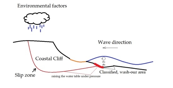
Weather conditions are of the greatest importance for slip zone creation. Extreme weather conditions in the Baltic Sea are observed increasingly often; therefore, the erosive action can be expected to worsen [53,54,55,56,57,58,59]. The geological structure of the area is characterised by very low permeability. Drainages have been made in the most at risk locations, which reduces the amount of rainwater and increases the water table in the massif, without decreasing the scale of erosion. Some beaches have also been refilled by mechanically adding sand, which reduces the scale of the sea’s direct influence on the massif during storms. The environmental processes that occur in the study area are presented in Figure 13.
Effective coastal management in the southern Baltic calls for appropriate underwater monitoring. The sensitivity results obtained in this study indicate a local loss of stability for certain geotechnical parameters, which affect the massif as a whole. The previously calculated stability of the slope gives safe values [13], and the conclusion that the water table may be at different levels of the massif. The sensitivity of these parameters should be assessed to determine whether their change in an outcome of Factor of Safety will affect the final result. This approach is supported by the sensitivity calculations (e.g., in Figure 12 the change in parameter of Clay could affect the global stability of the cliff), which reveals that a potential change in only one parameter (e.g., due to water infiltration) may lead to a loss of stability.
Determining how groundwater infiltrates soil layers is crucial, as this causes the massif to slowly run off along the slope. The ALB technology demonstrated that in the places of the greatest negative changes (between two DTMs from autumn and winter), water may be introduced under this massif. This may occur during extreme weather conditions in the event of soil being washed out (Figure 11c,d) thereby creating a drainage through which water can enter. With the disappearance of the revs as natural breakwaters, upper geological irrigation and pressure are able to drain water under the slope, thereby causing erosion. This interpretation, resulting from the obtained bathymetric data and numerical calculations, requires further research into the dynamics of the sea in the Baltic area. If verified, it will be possible to formulate approaches for coastal monitoring, in terms of direct determination of factors causing degradation, and its application in similar areas.
The application of remote sensing techniques is useful to coastal research [36,79,80,81], the development of satellite techniques enables their use in different types of coasts. Most studies have focussed on determining and measuring trends of change [3,5,9,10,11,12,13,14,15,16]. This study aimed to evaluate the suitability of airborne bathymetry LiDAR in determining the factors causing coastal degradation, by combining topographic and bathymetric data. One of the most important aspects of this study, compared to previous studies, is the inclusion of numerical calculations on the sensitivity of geotechnical parameters to change. All factors that may cause such a change should be isolated, therefore ensuring that appropriate environmental management strategies are considered. Presenting this solution makes it possible to determine the results of degradation without the high costs of geotechnical research (especially for large areas). Furthermore, this study demonstrates the practical use of a bathymetric scanner, which has not been implemented before in the South Baltic Sea.
The ALB measurement methods outlined in this study have frequently been used for the precise determination of the sea floor. This study shows that the bathymetric scanning technology, equal to or exceeding the possibility of registering a Secchi depth of one, is the optimum technique for Baltic Sea monitoring. The use of alternative methods carries the risk of failing to register relevant sites, thus, rendering them impossible to analyse. This research shows that the optimum depth range of an ALB in the Baltic Sea is 5–8 m, which translates to approximately 1 km into the sea. Nevertheless, scanning technology below one Secchi disc and aerial photographs are useful for recording places with a sudden increase in depth, the level of vegetation in the water, or to process geometric profiles for geotechnical analyses.
The commercial use of ALB is rare (with only a very small group of technology recipients) and the proposed application is rather niche as it generates high costs compared with classical methods of aerial photogrammetry. Although cheaper methods are characterised by lower levels of precision and accuracy, or may register only the aquatic section, they still supply valuable information. The spatial comparison of two models confirms the possibility of a slip zone, which can explain the degradation of a cliff massif. This analysis provides information that is necessary for ensuring the safety of bathing areas and can be used to assess the degree of pollution, or as a foundation for developing maps of flood hazards and flood risks. It is worth investing in measurements using this technology, but the limits of this system, as discussed in this article, should be considered.
Bathymetric scanning has not found its application in coastal monitoring due to the burden of data volumes, data processing demands and requirements for direct application (e.g., in the perspective of using ALB technology in the Baltic Sea). In most cases, this refers to the hardware capabilities of the workstation, and the experience and knowledge of the person working with the data from ALB system. However, this article presents ways to encourage other researchers to use the ALB technology for different coastal types, through measurement planning, presenting automated processing, using raster instead of DTMs, or focusing on computing sensitivity of coastal stability. Moreover, methods of filtering these data can be used to reduce their weight, but the scope of methodology, in order not to lose spatial information, is a topic for further work on this technology.
The main goal of this article was to assess the suitability of topographic–bathymetric systems, in terms of their ability to monitor coastal changes. Given the identified shortcomings, when using the airborne bathymetry system, attention should be paid to the environmental conditions prior to measuring, and the cost of additional measurements. There are publications that help understand these data and how to deal with it [82]. When using cheaper methods, such as aerial photographs and a red scanner, the study can be divided into locations, characterised by the largest geometrical changes, and then measurements can be carried out under the water surface. This is a cheaper solution, but will not provide information on the swimming safety, or emerging revs and water circulation; therefore, the risk of possible coastal erosion could be overlooked.
As with laser scanning, which was not profitable (e.g., high cost of the device, weight of collected data), and yet still found various applications [83,84,85], bathymetric scanning will also be utilised in the analysis of the natural environment, rather than focusing on the technology itself. The data obtained can often discourage researchers, due to the required processing techniques. The article demonstrates that it is possible to develop them. Innovative applications will allow the development of, not only the technology itself, but also the entire region related to coastal protection. Another advantage of ALB technology is the ability to conduct multidisciplinary research, as demonstrated by this study, combining remote sensing techniques with geotechnics to identify and work towards solution of coastal management related e.g., in real estate [86].
Funding
Project data were obtained as part of the project “Creating a comprehensive system for registering the land zone of the coastal zone and the underwater part to a depth of 3 m” implemented by the company APEKS from the Regional Operational Program of the Pomeranian Voivodeship for 2014–2020 and financed with European Union funds.
Acknowledgments
The author would like to thank co-workers, Apeks Company and friends for their support throughout the research process. Credit goes to Journal Edit, whose editorial assistance improved the quality of the manuscript.
Conflicts of Interest
The author declares no conflict of interest.
References
- Global Climate Change. Available online: https://climate.nasa.gov/ (accessed on 5 February 2020).
- Hulley, G.; Shivers, S.; Wetherley, E.; Cudd, R. New ECOSTRESS and MODIS Land Surface Temperature Data Reveal Fine-Scale Heat Vulnerability in Cities: A Case Study for Los Angeles County, California. Remote Sens. 2019, 11, 2136. [Google Scholar] [CrossRef] [Green Version]
- Wu, X.; Xu, Q.; Li, G.; Liou, Y.-A.; Wang, B.; Mei, H.; Tong, K. Remotely-Observed Early Spring Warming in the Southwestern Yellow Sea Due to Weakened Winter Monsoon. Remote Sens. 2019, 11, 2478. [Google Scholar] [CrossRef] [Green Version]
- EU Strategy for the Baltic Sea Region (EUSBSR). Available online: https://www.balticsea-region-strategy.eu/about/implementation (accessed on 5 February 2020).
- Cosoli, S.; Pattiaratchi, C.; Hetzel, Y. High-Frequency Radar Observations of Surface Circulation Features along the South-Western Australian Coast. J. Mar. Sci. Eng. 2020, 8, 97. [Google Scholar] [CrossRef] [Green Version]
- Abu-Abdullah, M.M.; Youssef, A.M.; Maerz, N.H.; Abu-AlFadail, E.; Al-Harbi, H.M.; Al-Saadi, N.S. A Flood Risk Management Program of Wadi Baysh Dam on the Downstream Area: An Integration of Hydrologic and Hydraulic Models, Jizan Region, KSA. Sustainability 2020, 12, 1069. [Google Scholar] [CrossRef] [Green Version]
- Chen, M.; Nabih, S.; Brauer, N.S.; Gao, S.; Gourley, J.J.; Hong, Z.; Kolar, R.L.; Hong, Y. Can Remote Sensing Technologies Capture the Extreme Precipitation Event and Its Cascading Hydrological Response? A Case Study of Hurricane Harvey Using EF5 Modeling Framework. Remote Sens. 2020, 12, 445. [Google Scholar] [CrossRef] [Green Version]
- Daniela, R.; Ermanno, M.; Antonio, P.; Pasquale, R.; Marco, V. Assessment of Tuff Sea Cliff Stability Integrating Geological Surveys and Remote Sensing. Case History from Ventotene Island (Southern Italy). Remote Sens. 2020, 12, 2006. [Google Scholar] [CrossRef]
- Jaud, M.; Kervot, M.; Delacourt, C.; Bertin, S. Potential of Smartphone SfM Photogrammetry to Measure Coastal Morphodynamics. Remote Sens. 2019, 11, 2242. [Google Scholar] [CrossRef] [Green Version]
- Jaud, M.; Bertin, S.; Beauverger, M.; Augereau, E.; Delacourt, C. RTK GNSS-Assisted Terrestrial SfM Photogrammetry without GCP: Application to Coastal Morphodynamics Monitoring. Remote Sens. 2020, 12, 1889. [Google Scholar] [CrossRef]
- Zelaya Wziątek, D.; Terefenko, P.; Kurylczyk, A. Multi-Temporal Cliff Erosion Analysis Using Airborne Laser Scanning Surveys. Remote Sens. 2019, 11, 2666. [Google Scholar] [CrossRef] [Green Version]
- Terefenko, P.; Paprotny, D.; Giza, A.; Morales-Nápoles, O.; Kubicki, A.; Walczakiewicz, S. Monitoring Cliff Erosion with LiDAR Surveys and Bayesian Network-based Data Analysis. Remote Sens. 2019, 11, 843. [Google Scholar] [CrossRef] [Green Version]
- Ossowski, R.; Przyborski, M.; Tysiac, P. Stability Assessment of Coastal Cliffs Incorporating Laser Scanning Technology and a Numerical Analysis. Remote Sens. 2019, 11, 1951. [Google Scholar] [CrossRef] [Green Version]
- Santos, C.; Santos-Ferreira, A.; Dias, E. A Coastal Cliff Stability Study in Peniche (Portugal). In Engineering Geology for Society and Territory; Lollino, G., Ed.; Springer: Cham, Switzerland, 2015; Volume 2. [Google Scholar] [CrossRef]
- Martino, S.; Mazzanti, P. Analysis of sea cliff slope stability integrating traditional geomechanical surveys and remote sensing. Nat. Hazards Earth Syst. Sci. 2013, 1, 3689–3734. [Google Scholar] [CrossRef]
- Wolters, G.; Müller, G. Effect of Cliff Shape on Internal Stresses and Rock Slope Stability. J. Coast. Res. 2008, 24, 43–50. [Google Scholar] [CrossRef]
- Gege, P.; Dekker, A.G. Spectral and Radiometric Measurement Requirements for Inland, Coastal and Reef Waters. Remote Sens. 2020, 12, 2247. [Google Scholar] [CrossRef]
- Garcia, R.A.; Lee, Z.; Hochberg, E.J. Hyperspectral Shallow-Water Remote Sensing with an Enhanced Benthic Classifier. Remote Sens. 2018, 10, 147. [Google Scholar] [CrossRef] [Green Version]
- Zhou, X.; Marani, M.; Albertson, J.D.; Silvestri, S. Hyperspectral and Multispectral Retrieval of Suspended Sediment in Shallow Coastal Waters Using Semi-Analytical and Empirical Methods. Remote Sens. 2017, 9, 393. [Google Scholar] [CrossRef] [Green Version]
- Janowski, L.; Madricardo, F.; Fogarin, S.; Kruss, A.; Molinaroli, E.; Kubowicz-Grajewska, A.; Tegowski, J. Spatial and Temporal Changes of Tidal Inlet Using Object-Based Image Analysis of Multibeam Echosounder Measurements: A Case from the Lagoon of Venice, Italy. Remote Sens. 2020, 12, 2117. [Google Scholar] [CrossRef]
- Tyllianakis, E.; Fronkova, L.; Posen, P.; Luisetti, T.; Chai, S.M. Mapping Ecosystem Services for Marine Planning: A UK Case Study. Resources 2020, 9, 40. [Google Scholar] [CrossRef]
- Karim, F.; Marvanek, S.; Merrin, L.E.; Nielsen, D.; Hughes, J.; Stratford, D.; Pollino, C. Modelling Flood-Induced Wetland Connectivity and Impacts of Climate Change and Dam. Water 2020, 12, 1278. [Google Scholar] [CrossRef]
- Abderrezzak, K.; Paquir, A.; Mignot, E. Modelling flash flood propagation in urban areas using a two-dimensional numerical model. Nat. Hazards 2008, 50, 433–460. [Google Scholar] [CrossRef]
- Apel, H.; Aronica, G.T.; Kreibich, H.; Thieken, A.H. Flood risk analyses—How detailed do we need to be? Nat. Hazards 2009, 49, 79–98. [Google Scholar] [CrossRef]
- Bates, P.D.; De Roo, A.P.J. A simple raster-based model for flood inundation simulation. J. Hydrol. 2000, 236, 54–77. [Google Scholar] [CrossRef]
- Wang, H.; Zhao, H. Dynamic Changes of Soil Erosion in the Taohe River Basin Using the RUSLE Model and Google Earth Engine. Water 2020, 12, 1293. [Google Scholar] [CrossRef]
- Zwolak, K.; Wigley, R.; Bohan, A.; Zarayskaya, Y.; Bazhenova, E.; Dorshow, W.; Sumiyoshi, M.; Sattiabaruth, S.; Roperez, J.; Proctor, A.; et al. The Autonomous Underwater Vehicle Integrated with the Unmanned Surface Vessel Mapping the Southern Ionian Sea. The Winning Technology Solution of the Shell Ocean Discovery XPRIZE. Remote Sens. 2020, 12, 1344. [Google Scholar] [CrossRef] [Green Version]
- Stateczny, A.; Błaszczak-Bąk, W.; Sobieraj-Żłobińska, A.; Motyl, W.; Wisniewska, M. Methodology for Processing of 3D Multibeam Sonar Big Data for Comparative Navigation. Remote Sens. 2019, 11, 2245. [Google Scholar] [CrossRef] [Green Version]
- Jung, J.; Li, J.; Choi, H.; Myung, H. Localization of AUVs using visual information of underwater structures and artificial landmarks. Intell. Serv. Robot. 2017, 10, 67–76. [Google Scholar] [CrossRef]
- Li, Y.; Ma, T.; Wang, R.; Chen, P.; Shen, P.; Jiang, Y. Terrain Matching Positioning Method Based on Node Multi-information Fusion. J. Navig. 2017, 70, 82–100. [Google Scholar] [CrossRef]
- Lyzenga, D.R. Remote sensing of bottom reflectance and water attenuation parameters in shallow water using aircraft and Landsat data. Int. J. Remote Sens. 1981, 2, 71–82. [Google Scholar] [CrossRef]
- Lyzenga, D.R. Passive remote sensing technique for mapping water depth. Appl. Opt. 1978, 17, 379–383. [Google Scholar] [CrossRef]
- Chybicki, A. Mapping South Baltic Near-Shore Bathymetry Using Sentinel-2 Observations. Pol. Marit. Res. 2017, 24, 15–25. [Google Scholar] [CrossRef]
- Saleem, A.; Awange, J.L. Coastline shift analysis in data deficient regions: Exploiting the high spatio-temporal resolution Sentinel-2 products. CATENA 2019, 179, 6–19. [Google Scholar] [CrossRef] [Green Version]
- Nazeer, M.; Waqas, M.; Shahzad, M.I.; Zia, I.; Wu, W. Coastline Vulnerability Assessment through Landsat and Cubesats in a Coastal Mega City. Remote Sens. 2020, 12, 749. [Google Scholar] [CrossRef] [Green Version]
- Zanutta, A.; Lambertini, A.; Vittuari, L. UAV Photogrammetry and Ground Surveys as a Mapping Tool for Quickly Monitoring Shoreline and Beach Changes. J. Mar. Sci. Eng. 2020, 8, 52. [Google Scholar] [CrossRef] [Green Version]
- Specht, M.; Specht, C.; Mindykowski, J.; Dąbrowski, P.; Maśnicki, R.; Makar, A. Geospatial Modeling of the Tombolo Phenomenon in Sopot using Integrated Geodetic and Hydrographic Measurement Methods. Remote Sens. 2020, 12, 737. [Google Scholar] [CrossRef] [Green Version]
- Yu, Q.; Wang, Q.; Yan, X.; Yang, T.; Song, S.; Yao, M.; Zhou, K.; Huang, X. Ground Deformation of the Chongming East Shoal Reclamation Area in Shanghai Based on SBAS-InSAR and Laboratory Tests. Remote Sens. 2020, 12, 1016. [Google Scholar] [CrossRef] [Green Version]
- Zhang, Y.; Hou, X. Characteristics of Coastline Changes on Southeast Asia Islands from 2000 to 2015. Remote Sens. 2020, 12, 519. [Google Scholar] [CrossRef] [Green Version]
- Maune, D. (Ed.) Digital Elevation Model Technologies and Applications: The DEM User’s Manual, 2nd ed.; American Society for Photogrammetry and Remote Sensing: Bethesda, MD, USA, 2007; pp. 253–329. [Google Scholar]
- Kinzel, P.J.; Wright, C.W.; Nelson, J.M.; Burman, A.R. Evaluation of an experimental LiDAR for surveying a shallow, braided, sand-bedded river. J. Hydraul. Eng. 2007, 133, 838–842. [Google Scholar] [CrossRef] [Green Version]
- Tonina, D.; McKean, J.A.; Benjankar, R.M.; Wright, C.W.; Goode, J.R.; Chen, Q.; Reeder, W.J.; Carmichael, R.A.; Edmondson, M.R. Mapping river bathymetries: Evaluating topobathymetric LiDAR survey. Earth Surf. Process. Landf. 2019, 44, 507–520. [Google Scholar] [CrossRef]
- Genchi, S.A.; Vitale, A.J.; Perillo, G.M.E.; Seitz, C.; Delrieux, C.A. Mapping Topobathymetry in a Shallow Tidal Environment Using Low-Cost Technology. Remote Sens. 2020, 12, 1394. [Google Scholar] [CrossRef]
- Kasvi, E.; Salmela, J.; Lotsari, E.; Kumpula, T.; Lane, S.N. Comparison of remote sensing based approaches for mapping bathymetry of shallow, clear water rivers. Geomorphology 2019, 333, 180–197. [Google Scholar] [CrossRef]
- Alvarez, L.V.; Moreno, H.A.; Segales, A.R.; Pham, T.G.; Pillar-Little, E.A.; Chilson, P.B. Merging Unmanned Aerial Systems (UAS) Imagery and Echo Soundings with an Adaptive Sampling Technique for Bathymetric Surveys. Remote Sens. 2018, 10, 1362. [Google Scholar] [CrossRef] [Green Version]
- Esposito, G.; Salvini, R.; Matano, F.; Sacchi, M.; Danzi, M.; Somma, R.; Troise, C. Multitemporal monitoring of a coastal landslide through SfM-derived point cloud comparison. Photogramm. Rec. 2017, 32, 459–479. [Google Scholar] [CrossRef] [Green Version]
- Taramelli, A.; Cappucci, S.; Valentini, E.; Rossi, L.; Lisi, I. Nearshore Sandbar Classification of Sabaudia (Italy) with LiDAR Data: The FHyL Approach. Remote Sens. 2020, 12, 1053. [Google Scholar] [CrossRef] [Green Version]
- Burdziakowski, P.; Tysiac, P. Combined Close Range Photogrammetry and Terrestrial Laser Scanning for Ship Hull Modelling. Geosciences 2019, 9, 242. [Google Scholar] [CrossRef] [Green Version]
- Agrafiotis, P.; Karantzalos, K.; Georgopoulos, A.; Skarlatos, D. Correcting Image Refraction: Towards Accurate Aerial Image-Based Bathymetry Mapping in Shallow Waters. Remote Sens. 2020, 12, 322. [Google Scholar] [CrossRef] [Green Version]
- Bué, I.; Catalão, J.; Semedo, Á. Intertidal Bathymetry Extraction with Multispectral Images: A Logistic Regression Approach. Remote Sens. 2020, 12, 1311. [Google Scholar] [CrossRef] [Green Version]
- Mandlburger, G.; Pfennigbauer, M.; Schwarz, R.; Flöry, S.; Nussbaumer, L. Concept and Performance Evaluation of a Novel UAV-Borne Topo-Bathymetric LiDAR Sensor. Remote Sens. 2020, 12, 986. [Google Scholar] [CrossRef] [Green Version]
- Gallina, V.; Torresan, S.; Zabeo, A.; Critto, A.; Glade, T.; Marcomini, A. A Multi-Risk Methodology for the Assessment of Climate Change Impacts in Coastal Zones. Sustainability 2020, 12, 3697. [Google Scholar] [CrossRef]
- Carlsson, M. Sea Level and Salinity Variations in the Baltic Sea—An Oceanographic Study Using Historical Data. Ph.D. Thesis, Gothenborg University, Gothenburg, Sweden, 1997. [Google Scholar]
- Elken, J.; Matthäus, W. Baltic Sea oceanography. In The BACC Author Team: Assessment of Climate Change for the Baltic Sea Basin; Springer: Berlin, Germany, 2008; pp. 379–385. [Google Scholar]
- Reusch, T.B.H.; Dierking, J.; Andersson, H.C.; Bonsdorff, E.; Carstensen, J.; Casini, M.; Casini, M.; Czajkowski, M.; Hasler, B.; Hinsby, K.; et al. The Baltic Sea as a time machine for the future coastal ocean. Sci. Adv. 2018, 4. [Google Scholar] [CrossRef] [Green Version]
- Wolski, T.; Wiśniewski, B. Long-Term, Seasonal and Short-Term Fluctuations in the Water Level of the Southern Baltic Sea. Quaest. Geogr. 2014, 33, 181–197. [Google Scholar] [CrossRef] [Green Version]
- Girjatowicz, J.; Swiatek, M.; Wolski, T. The influence of atmospheric circulation on the water level on the southern coast of the Baltic Sea. Int. J. Climatol. 2016, 36. [Google Scholar] [CrossRef]
- Climate Classification. Available online: https://www.britannica.com/science/Koppen-climate-classification (accessed on 2 September 2020).
- Polish Institute of Meteorology and Water Management-National Research Institute, Maritime Branch in Gdynia: The Assessment of the Impact of Current and Future Climate Change in the Polish Zone and the Ecosystem of the Baltic Sea, Gdynia. 2014. Available online: https://nfosigw.gov.pl/download/gfx/nfosigw/pl/nfoekspertyzy/858/210/1/2014-424.pdf (accessed on 2 September 2020).
- Live Cam. Available online: http://mlb.ibwpan.gda.pl/index.php/pl/camera/ (accessed on 20 June 2020).
- Numerical Forecast. Available online: https://meteopg.pl/#/ (accessed on 20 June 2020).
- Wu, D.; Phinn, S.; Johansen, K.; Robson, A.; Muir, J.; Searle, C. Estimating Changes in Leaf Area, Leaf Area Density, and Vertical Leaf Area Profile for Mango, Avocado, and Macadamia Tree Crowns Using Terrestrial Laser Scanning. Remote Sens. 2018, 10, 1750. [Google Scholar]
- Agrafiotis, P.; Skarlatos, D.; Georgopoulos, A.; Karantzalos, K. DepthLearn: Learning to Correct the Refraction on Point Clouds Derived from Aerial Imagery for Accurate Dense Shallow Water Bathymetry Based on SVMs-Fusion with LiDAR Point Clouds. Remote Sens. 2019, 11, 2225. [Google Scholar]
- Agrafiotis, P.; Skarlatos, D.; Georgopoulos, A.; Karantzalos, K. Shallow Water Bathymetry Mapping from Uav Imagery Based on Machine Learning. Int. Arch. Photogramm. Remote Sens. Spatial Inf. Sci. 2019, XLII-2/W10, 9–16. [Google Scholar]
- Xiong, L.; Wang, G.; Bao, Y.; Zhou, X.; Wang, K.; Liu, H.; Sun, X.; Zhao, R. A Rapid Terrestrial Laser Scanning Method for Coastal Erosion Studies: A Case Study at Freeport, Texas, USA. Sensors 2019, 19, 3252. [Google Scholar] [CrossRef] [PubMed] [Green Version]
- Hu, B.; Chen, J.; Zhang, X. Monitoring the Land Subsidence Area in a Coastal Urban Area with InSAR and GNSS. Sensors 2019, 19, 3181. [Google Scholar] [CrossRef] [PubMed] [Green Version]
- Mancini, F.; Castagnetti, C.; Rossi, P.; Dubbini, M.; Fazio, N.L.; Perrotti, M.; Lollino, P. An Integrated Procedure to Assess the Stability of Coastal Rocky Cliffs: From UAV Close-Range Photogrammetry to Geomechanical Finite Element Modeling. Remote Sens. 2017, 9, 1235. [Google Scholar]
- Morgenstern, N.R.; Price, V.E. The analysis of the stability of general slip surfaces. Geotechnique 1965, 15, 79–93. [Google Scholar] [CrossRef]
- Abd-Elaty, I.; Eldeeb, H.; Vranayova, Z.; Zelenakova, M. Stability of Irrigation Canal Slopes Considering the Sea Level Rise and Dynamic Changes: Case Study El-Salam Canal, Egypt. Water 2019, 11, 1046. [Google Scholar]
- Han, X.; Jin, J.; Wang, M.; Jiang, W. Guided 3D point cloud filtering. Multimed. Tools Appl. 2017, 77, 17397–17411. [Google Scholar] [CrossRef]
- Butler, J.B.; Lane, S.N.; Chandler, J.H.; Porfiri, E. Through-water close range digital photogrammetry in flume and field environments. Photogramm. Rec. 2002, 17, 419–439. [Google Scholar] [CrossRef]
- Fryer, J.F. Photogrammetry through shallow waters. Aust. J. Geod. Photogramm. Surv. 1983, 38, 25–38. [Google Scholar]
- Bugajny, N.; Furmańczyk, K. Comparison of Short-Term Changes Caused by Storms along Natural and Protected Sections of the Dziwnow Spit, Southern Baltic Coast. J. Coast. Res. 2017, 33, 775–785. [Google Scholar] [CrossRef]
- Bugajny, N.; Furmańczyk, K. Dune coast changes caused by weak storm events in Miedzywodzie, Poland. J. Coast. Res. 2014, 70, 211–216. [Google Scholar] [CrossRef]
- Kaszubowski, L.; Coufal, R. Engineering-Geological Analysis of the Polish Baltic Sea Bottom; Biuletyn-Państwowego Instytutu Geologicznego: Warsaw, Poland, 2011; Volume 446, pp. 341–349. [Google Scholar]
- Szmytkiewicz, M.; Biegowski, J.; Kaczmarek, L.M.; Okrój, T.; Ostrowski, R.; Pruszak, Z.; Różyńsky, G.; Skaja, M. Coastline changes nearby harbour structures: Comparative analysis of one-line models versus field data. Coast. Eng. 2000, 40, 119–139. [Google Scholar] [CrossRef]
- Hampton, M.A.; Griggs, G. Formation, Evolution, and Stability of Coastal Cliffs-Status and Trends. U.S. Geological Survey Professional Paper 1693. Available online: https://pubs.usgs.gov/pp/pp1693/ (accessed on 12 November 2020).
- Arkin, Y.; Michaeli, L. Short-and long-term erosional processes affecting the stability of the Mediterranean coastal cliffs of Israel. Eng. Geol. 1985, 21, 153–174. [Google Scholar] [CrossRef]
- Hoque, M.A.; Pollard, W.H. Pollard, Stability of permafrost dominated coastal cliffs in the Arctic. Polar Sci. 2016, 10, 79–88. [Google Scholar] [CrossRef]
- Kroon, A.; Davidson, M.A.; Aarninkhof, S.G.J.; Archetti, R.; Armaroli, C.; Gonzalez, M.; Medri, S.; Osorio, A.; Aagaard, T.; Holman, R.A.; et al. Application of remote sensing video systems to coastline management problems. Coast. Eng. 2007, 54, 493–505. [Google Scholar] [CrossRef]
- Sui, L.; Wang, J.; Yang, X.; Wang, Z. Spatial-Temporal Characteristics of Coastline Changes in Indonesia from 1990 to 2018. Sustainability 2020, 12, 3242. [Google Scholar] [CrossRef] [Green Version]
- Kogut, T.; Bakuła, K. Improvement of Full Waveform Airborne Laser Bathymetry Data Processing based on Waves of Neighborhood Points. Remote Sens. 2019, 11, 1255. [Google Scholar] [CrossRef] [Green Version]
- Suchocki, C.; Damięcka-Suchocka, M.; Katzer, J.; Janicka, J.; Rapiński, J.; Stałowska, P. Remote Detection of Moisture and Bio-Deterioration of Building Walls by Time-Of-Flight and Phase-Shift Terrestrial Laser Scanners. Remote Sens. 2020, 12, 1708. [Google Scholar] [CrossRef]
- Binczyk, M.; Kalitowski, P.; Szulwic, J.; Tysiac, P. Nondestructive Testing of the Miter Gates Using Various Measurement Methods. Sensors 2020, 20, 1749. [Google Scholar] [CrossRef] [PubMed] [Green Version]
- Miśkiewicz, M.; Pyrzowski, Ł.; Sobczyk, B. Short and Long Term Measurements in Assessment of FRP Composite Footbridge Behavior. Materials 2020, 13, 525. [Google Scholar] [CrossRef] [PubMed] [Green Version]
- Renigier-Biłozor, M.; Janowski, A.; D’Amato, M. Automated Valuation Model based on fuzzy and rough set theory for real estate market with insufficient source data. Land Use Policy 2019, 87, 104021. [Google Scholar] [CrossRef]
Figure 1.
(A) location of the sampling area within the southern Baltic Sea; (B) exact measurement locations outlined in black (source: OpenStreetMap).
Figure 1.
(A) location of the sampling area within the southern Baltic Sea; (B) exact measurement locations outlined in black (source: OpenStreetMap).

Figure 2.
Surveying techniques of (a) control points on the measured terrain, and (b) manual measurement of cross-sections in water using the Real Time Kinematic (RTK) Global Navigation Satellite System (GNSS) method.
Figure 2.
Surveying techniques of (a) control points on the measured terrain, and (b) manual measurement of cross-sections in water using the Real Time Kinematic (RTK) Global Navigation Satellite System (GNSS) method.

Figure 3.
Representation of Red–Green–Blue (RGB) images specifying the bathymetric scanning conditions on a five-point scale: (a) 1–2, cloud cover and large waves make topographic–bathymetric measurements unfeasible; (b) 2–3, increased sea level and high silting make topographic–bathymetric measurements unfeasible; (c) 3–4, where the appropriate weather conditions enable the photogrammetric mission to be completed, with a calm sea and a visible bottom at the shore being observed; and (d) 4–5, where the bottom is visible at a large distance from the shore.

Figure 4.
Comparison of results between point clouds, based on the distance between clearly identifiable objects from (a) the first flight; (b) the second flight; and (c) the third flight. Distances No. means the number for manual calculated distances between referenced point cloud and that measured in this experiment.


Figure 5.
Analysis of the obtained bathymetric scanning material: (a,c,e) the distance graph of the measured vertical offsets between the Airborne Bathymetry Lidar (ALB) method Digital Terrain Model (DTM) versus the DTM from the Central Geodetic Centre in Poland; and (b,d,f) a comparison between the results of manual measurements as a vertical offset between the GPS RTK measured point and DTM from ALB, from (a) and (b) the first measurement; (c) and (d) the second measurement; and (e) and (f) the third measurement. The colour palette indicates values from the lowest (marked in blue) to the highest (marked in red).

Figure 6.
Analysis of the obtained bottom extraction material from photos comparing the distance between (a) the measured digital terrain model (DTM) and the DTM from the Central Geodetic Centre in Poland; and (b) a comparison of the results of depth measurements to those made manually. The colour palette indicates values from the lowest (marked in blue) to the highest (marked in red).

Figure 7.
Processing scheme for selecting the optimal technique for use in areas with high environmental variability.
Figure 7.
Processing scheme for selecting the optimal technique for use in areas with high environmental variability.

Figure 8.
Bathymetry of the study area, acquired in conditions 4–5, with (a) a scanner performing a measurement up to a Secchi depth of 0.7; (b) aerial photographs; and (c) the height difference between these models.
Figure 8.
Bathymetry of the study area, acquired in conditions 4–5, with (a) a scanner performing a measurement up to a Secchi depth of 0.7; (b) aerial photographs; and (c) the height difference between these models.

Figure 9.
The difference in registration possibilities for the bathymetric scanner that is able to collect bottom information for (a) conditions 3–4; and (b) conditions 4–5.
Figure 9.
The difference in registration possibilities for the bathymetric scanner that is able to collect bottom information for (a) conditions 3–4; and (b) conditions 4–5.

Figure 10.
Result of the bathymetric scanner measurements of geometric differences before and after the autumn and winter season in (a) the northern part of the area; and (b) the south-eastern part.
Figure 10.
Result of the bathymetric scanner measurements of geometric differences before and after the autumn and winter season in (a) the northern part of the area; and (b) the south-eastern part.


Figure 11.
Identification of sites characterized by the largest positive change between Digital Terrain Models from ALB data from Autumn and Winter seasonal change (a,b) and the largest negative change between DTMs from Autumn and Winter seasonal change (c,d).
Figure 11.
Identification of sites characterized by the largest positive change between Digital Terrain Models from ALB data from Autumn and Winter seasonal change (a,b) and the largest negative change between DTMs from Autumn and Winter seasonal change (c,d).


Figure 12.
Sensitivity analysis for geotechnical parameters (Till (saclSi) (pink colour), Sandy Clay (saCl) (green colour), Clay (Cl) (purple colour), Clayey Sand (clSa) (blue colour), Fine Sand (FSa) (orange colour)) to identify the sensitivity of changes in parameters, the result of extreme weather conditions and the value of the safety factor. The red line indicate the value of Factor of Safety.

Figure 13.
The environmental situation of the studied area. During extreme weather conditions, in the event of soil being washed out (classified as the most negative change in Figure 11c,d), a drainage is created, through which water can enter, thus creating the slip zone.
Figure 13.
The environmental situation of the studied area. During extreme weather conditions, in the event of soil being washed out (classified as the most negative change in Figure 11c,d), a drainage is created, through which water can enter, thus creating the slip zone.


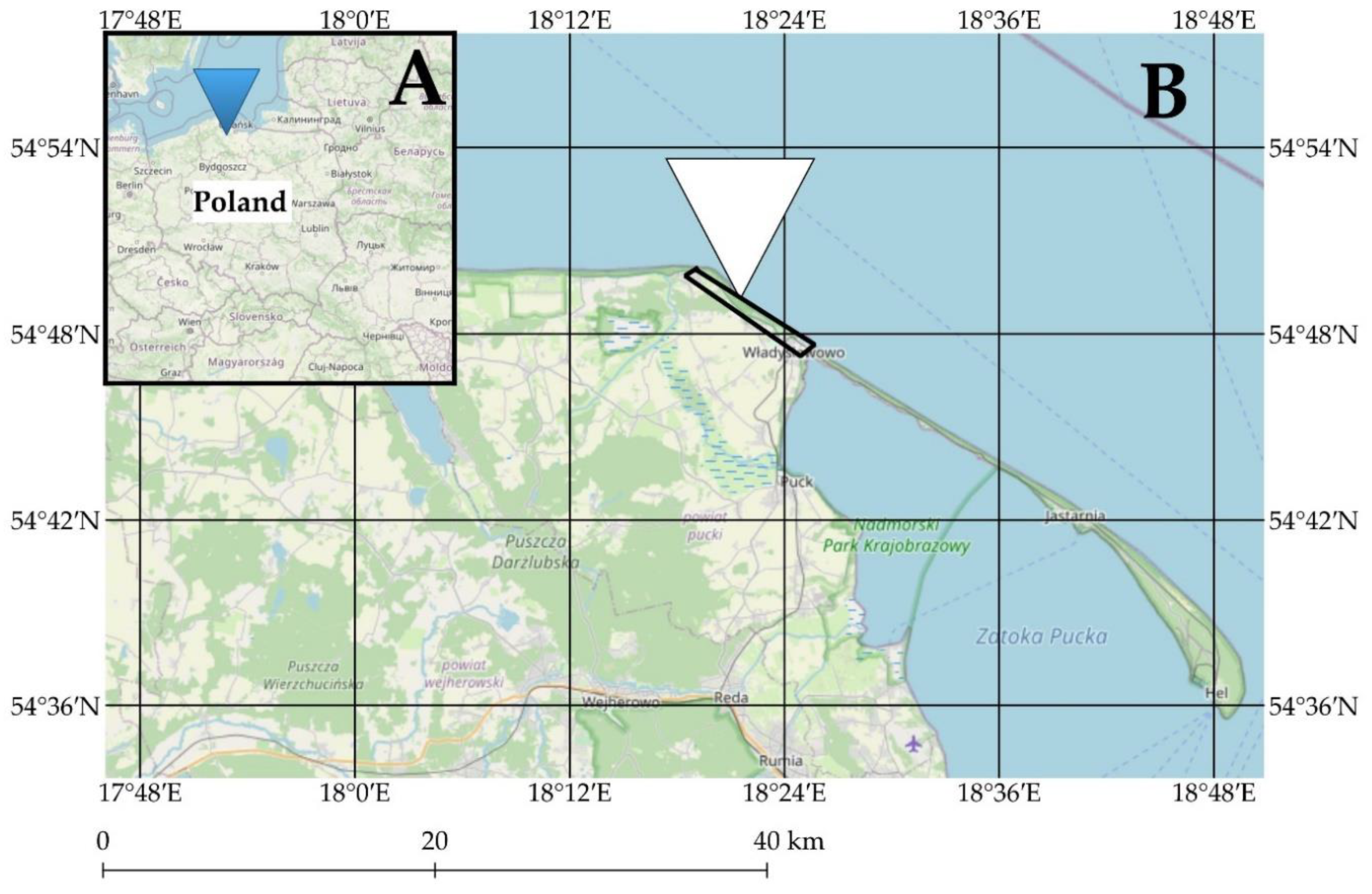
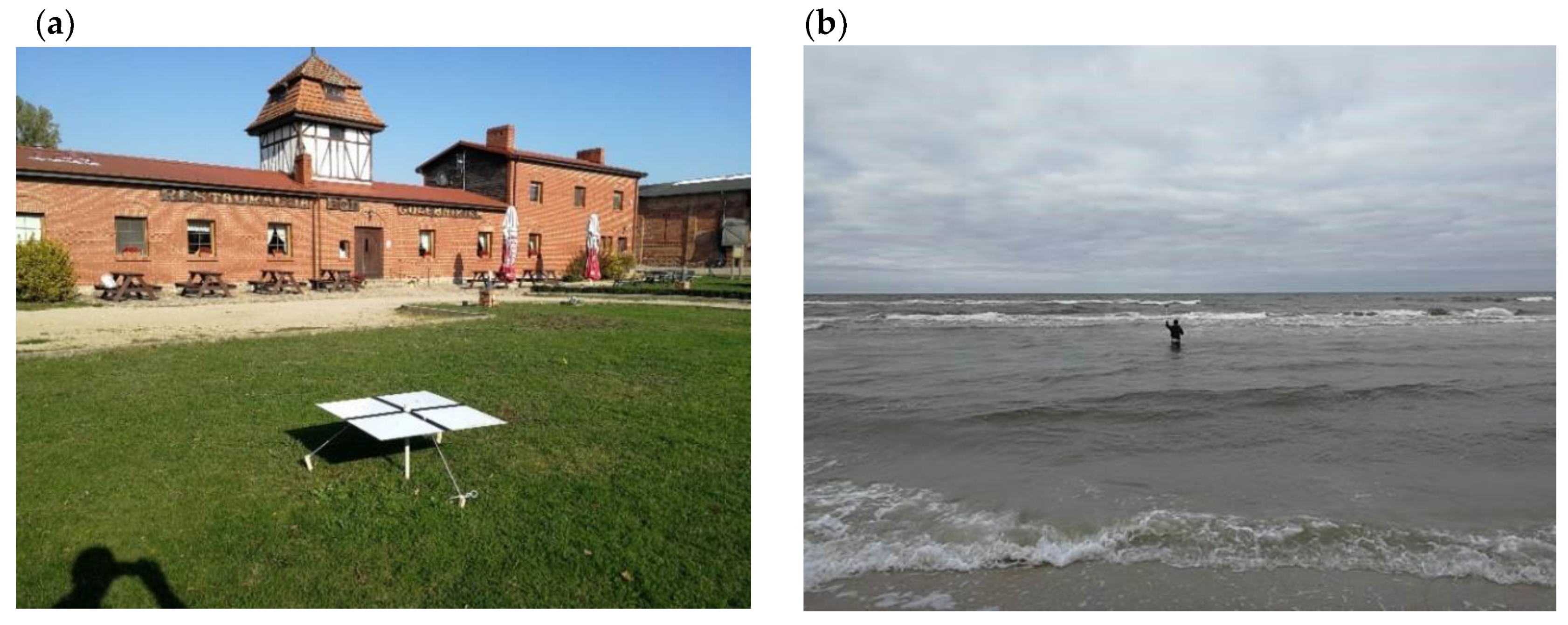
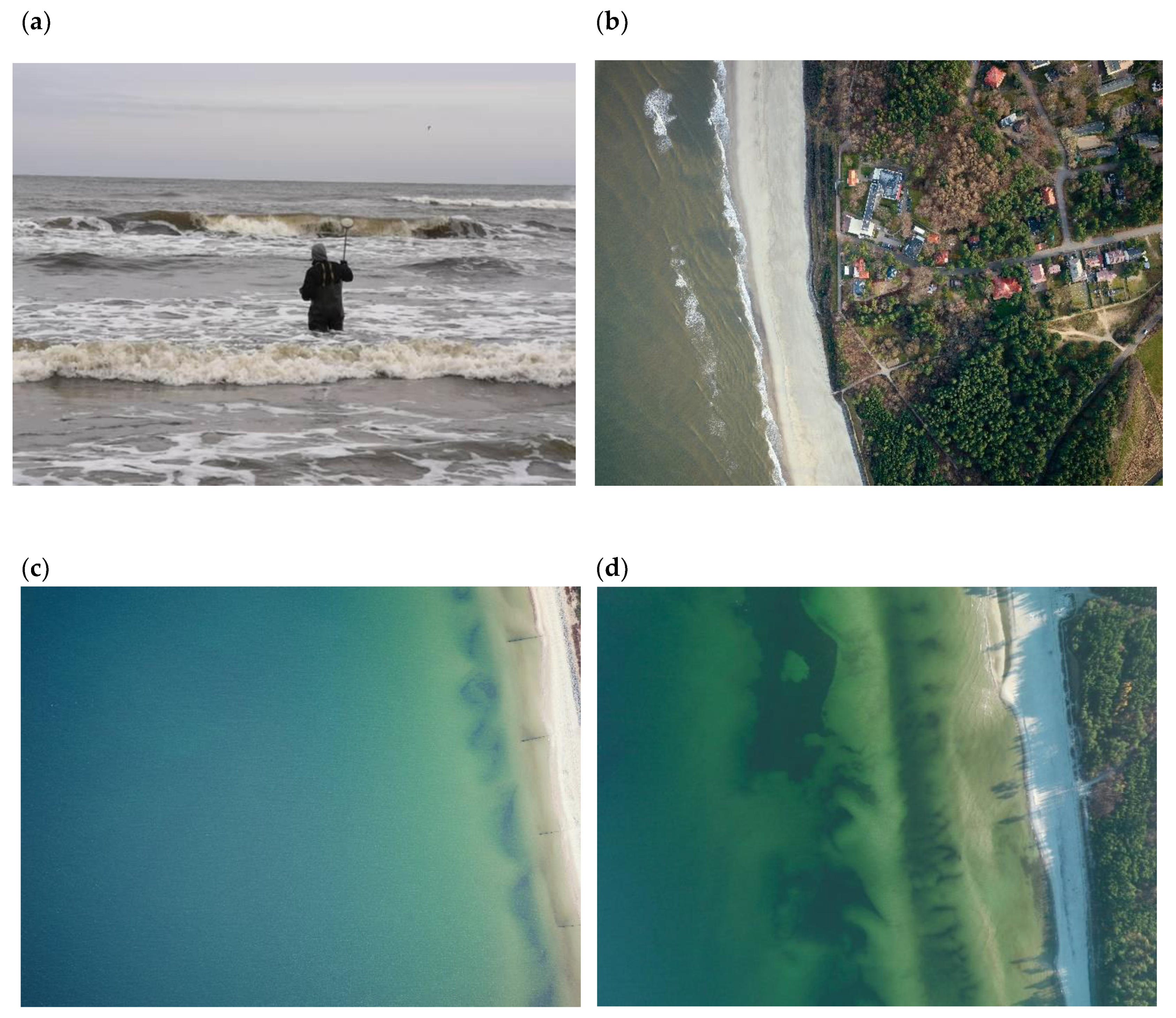
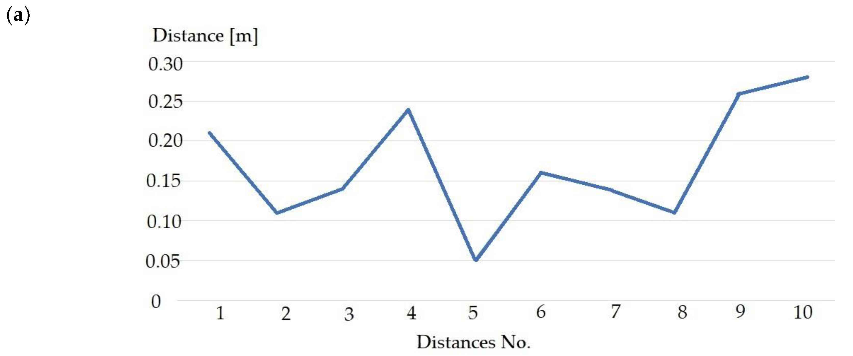
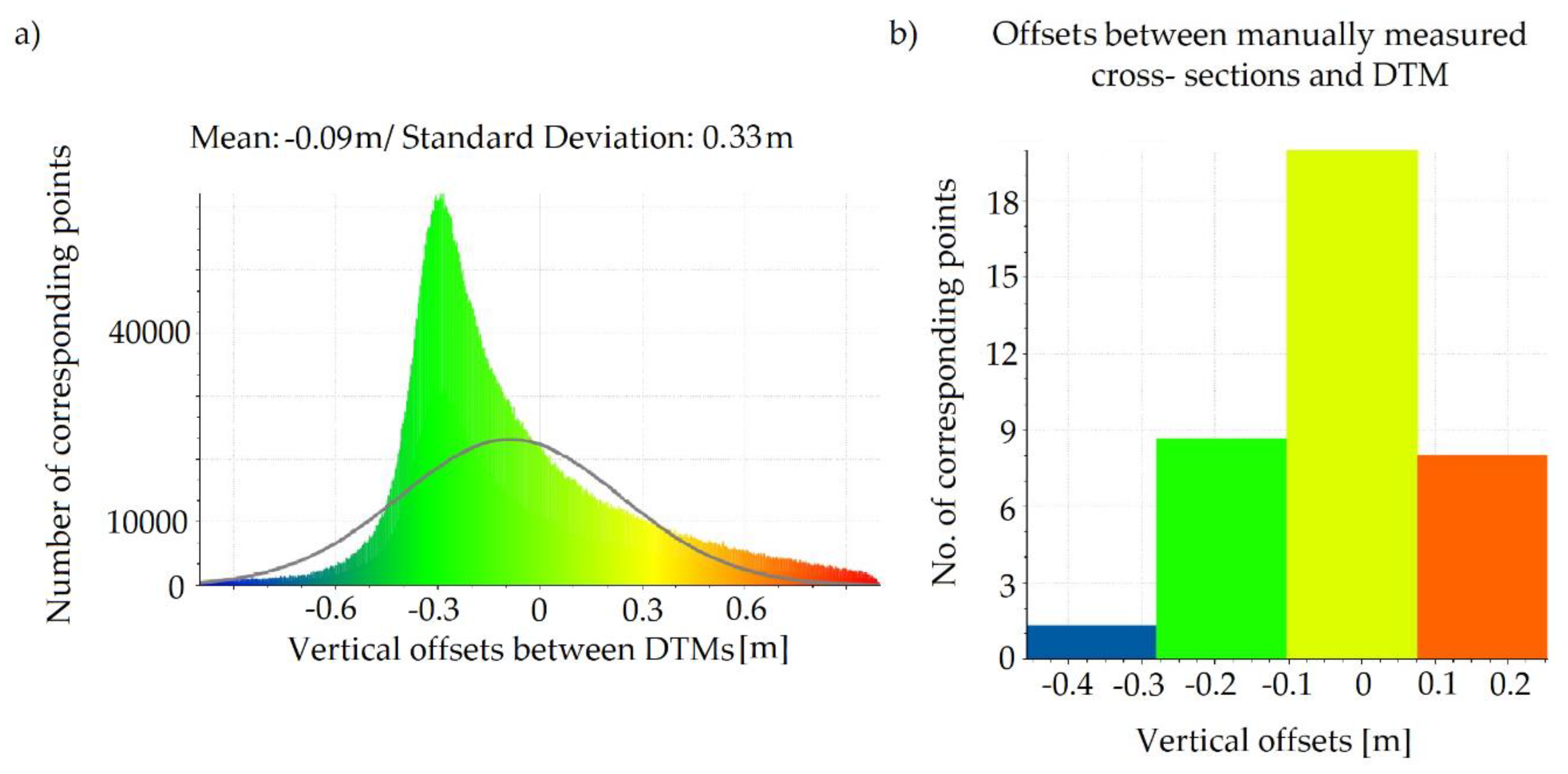
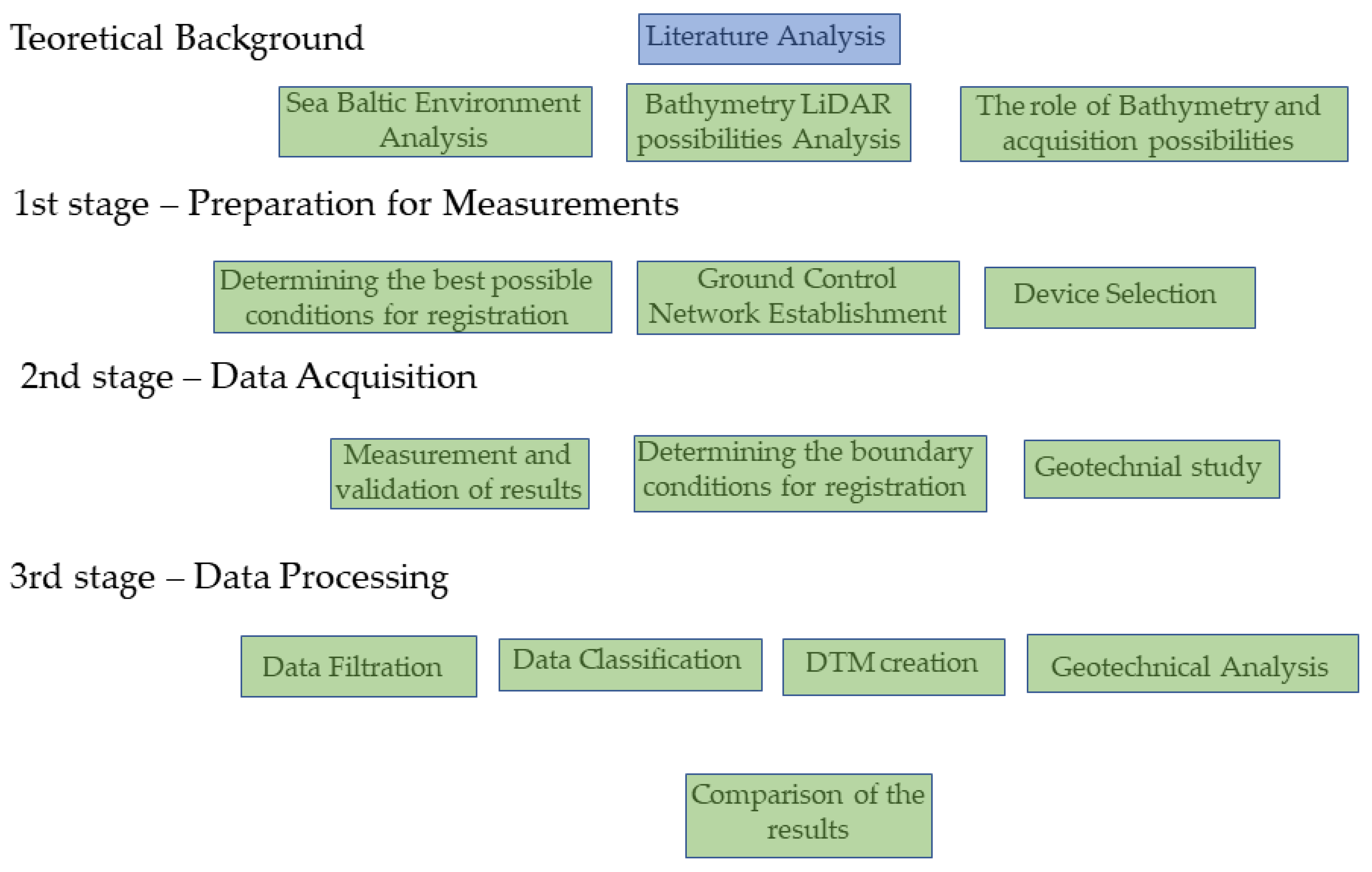
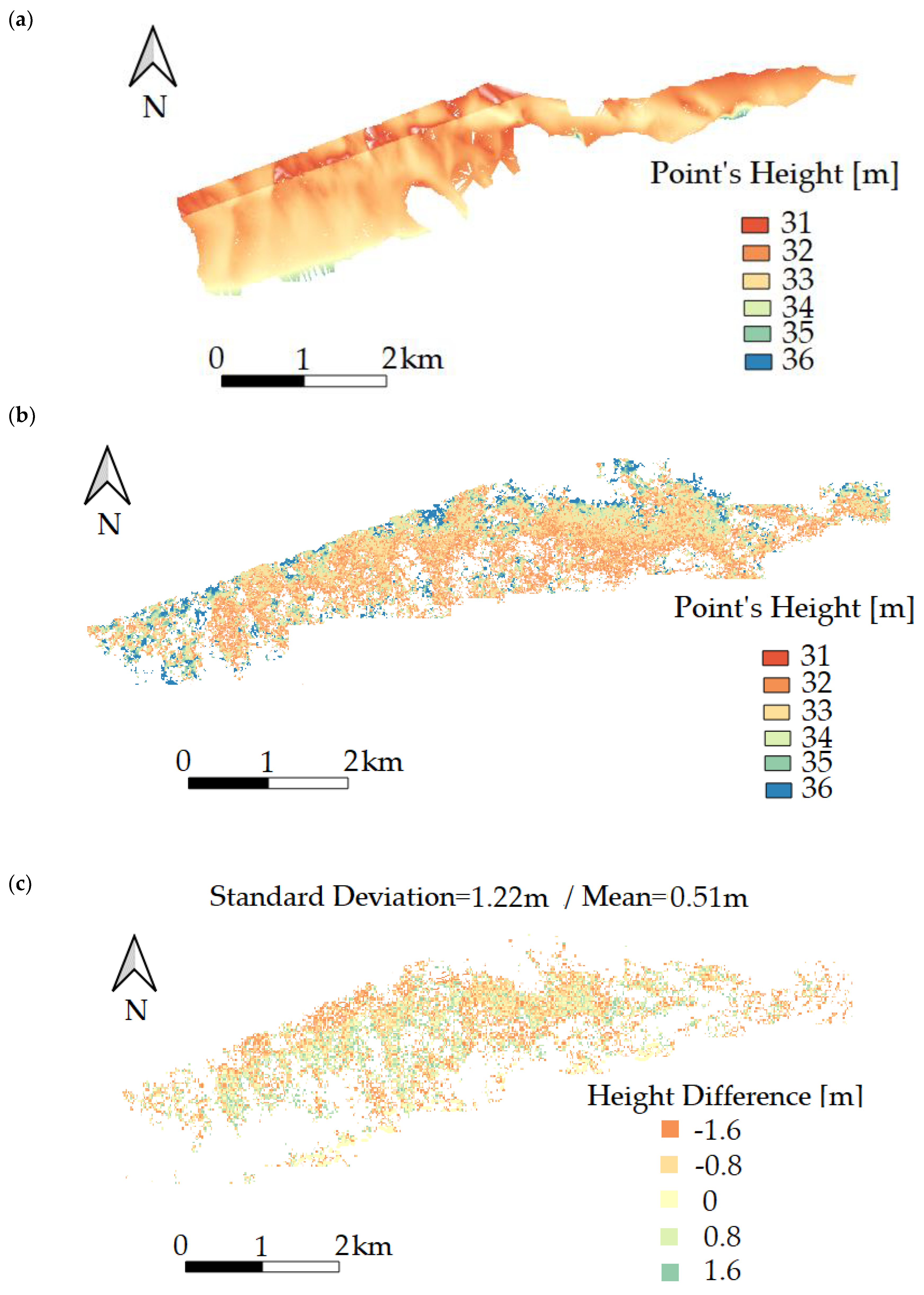
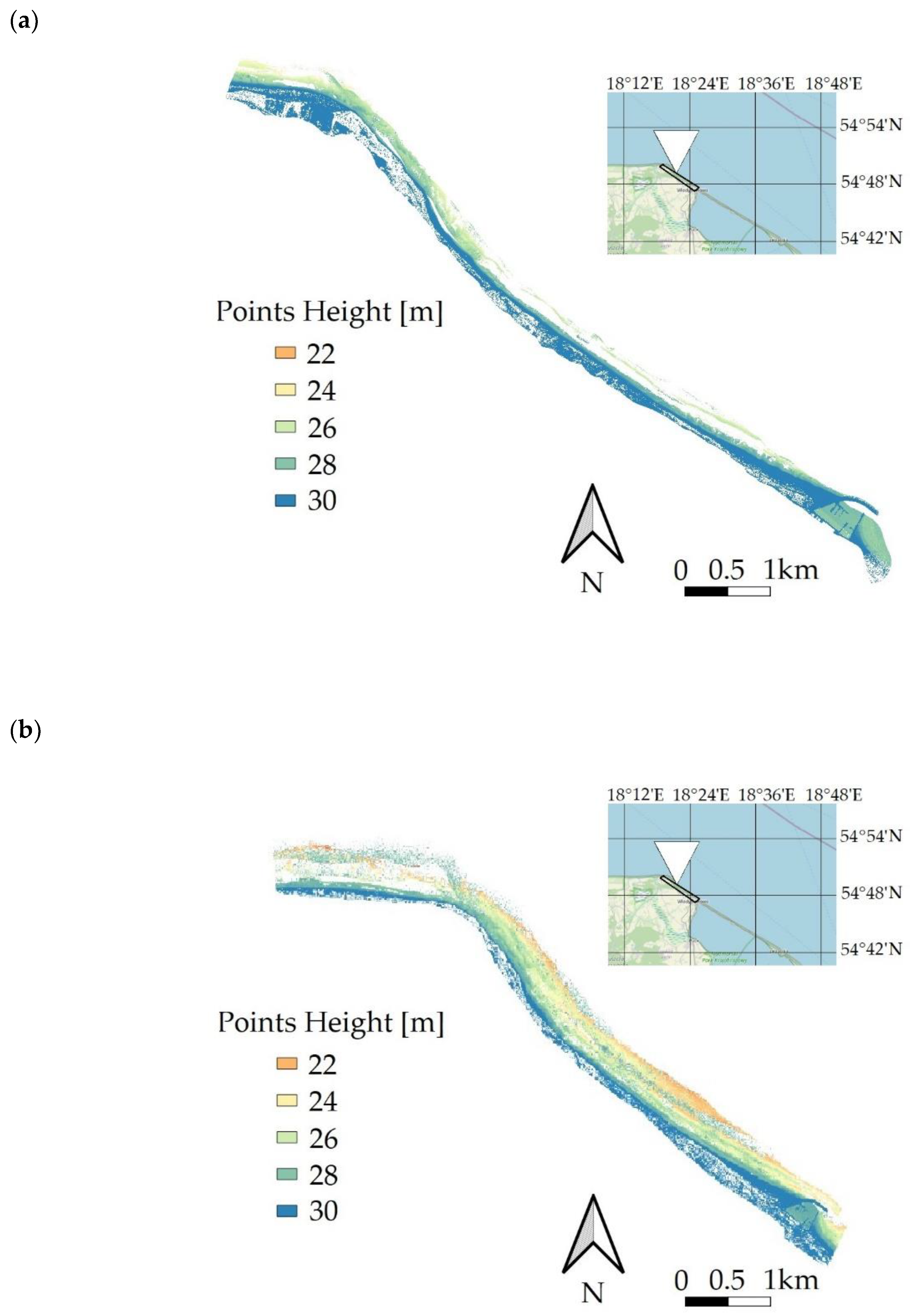
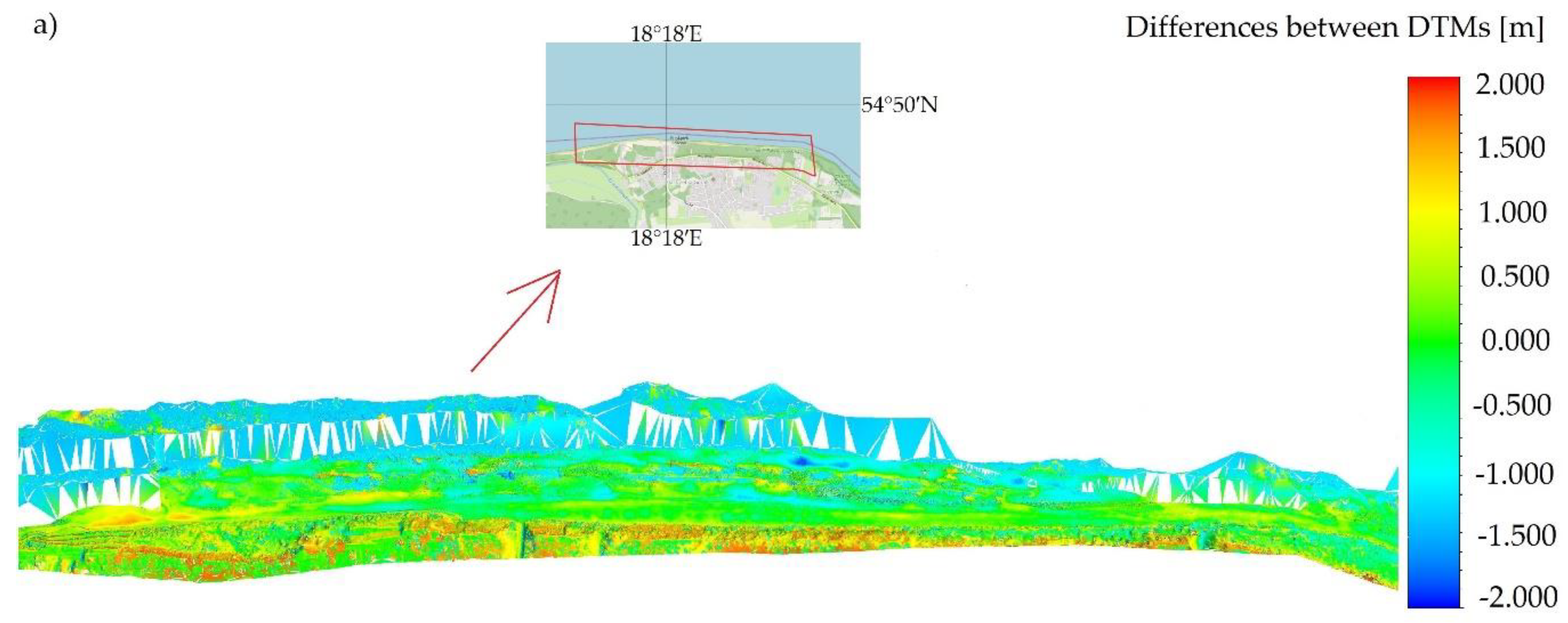
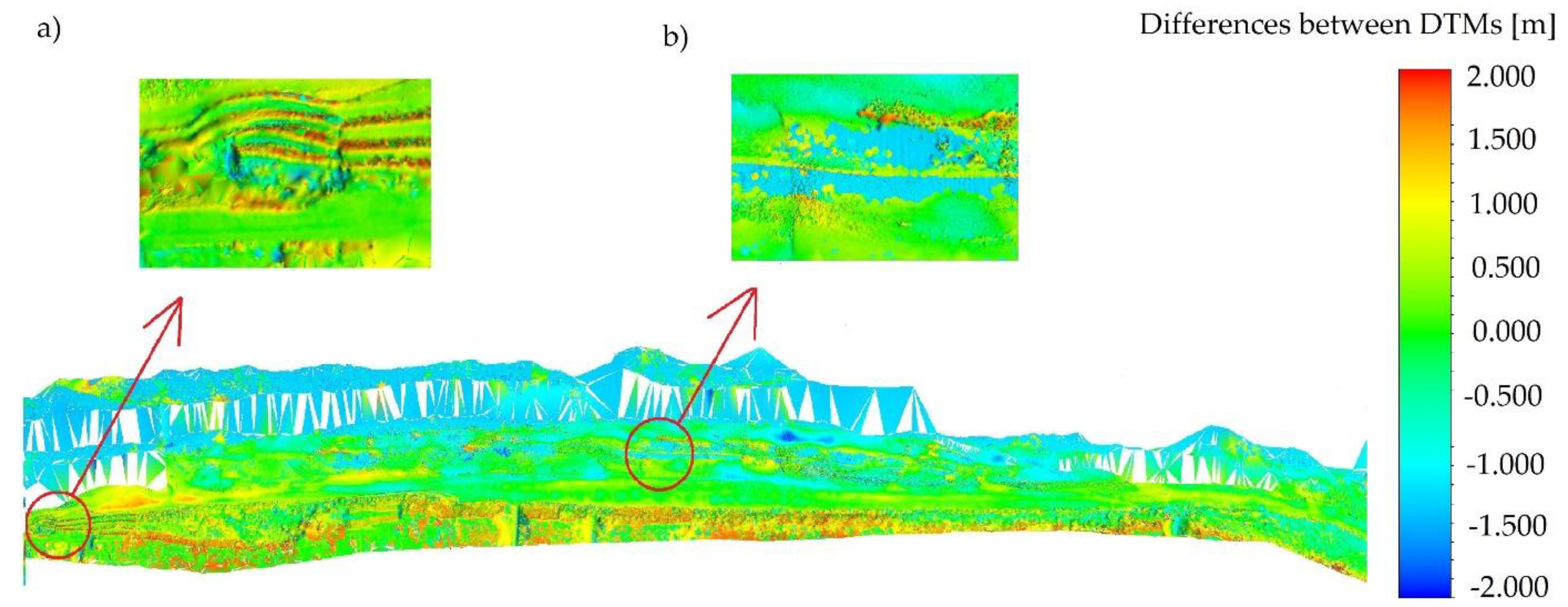
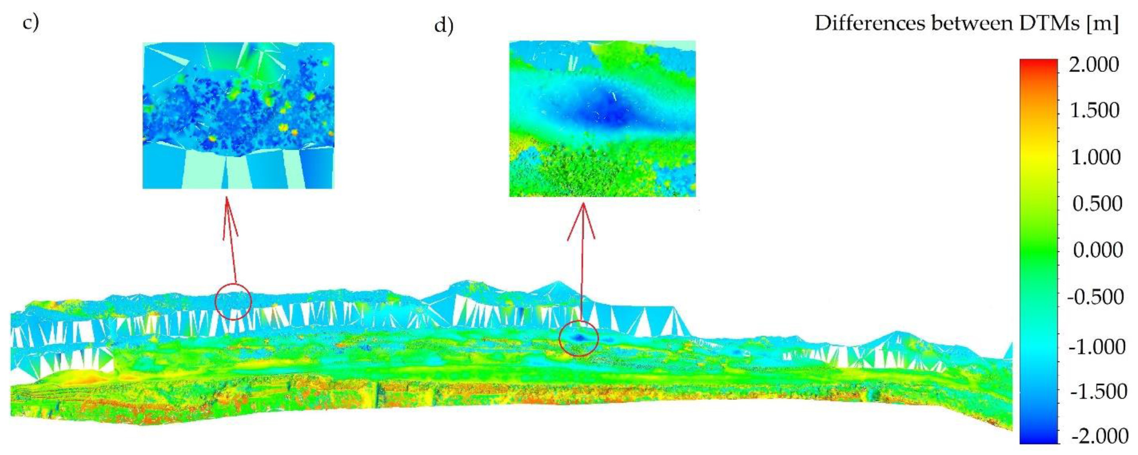
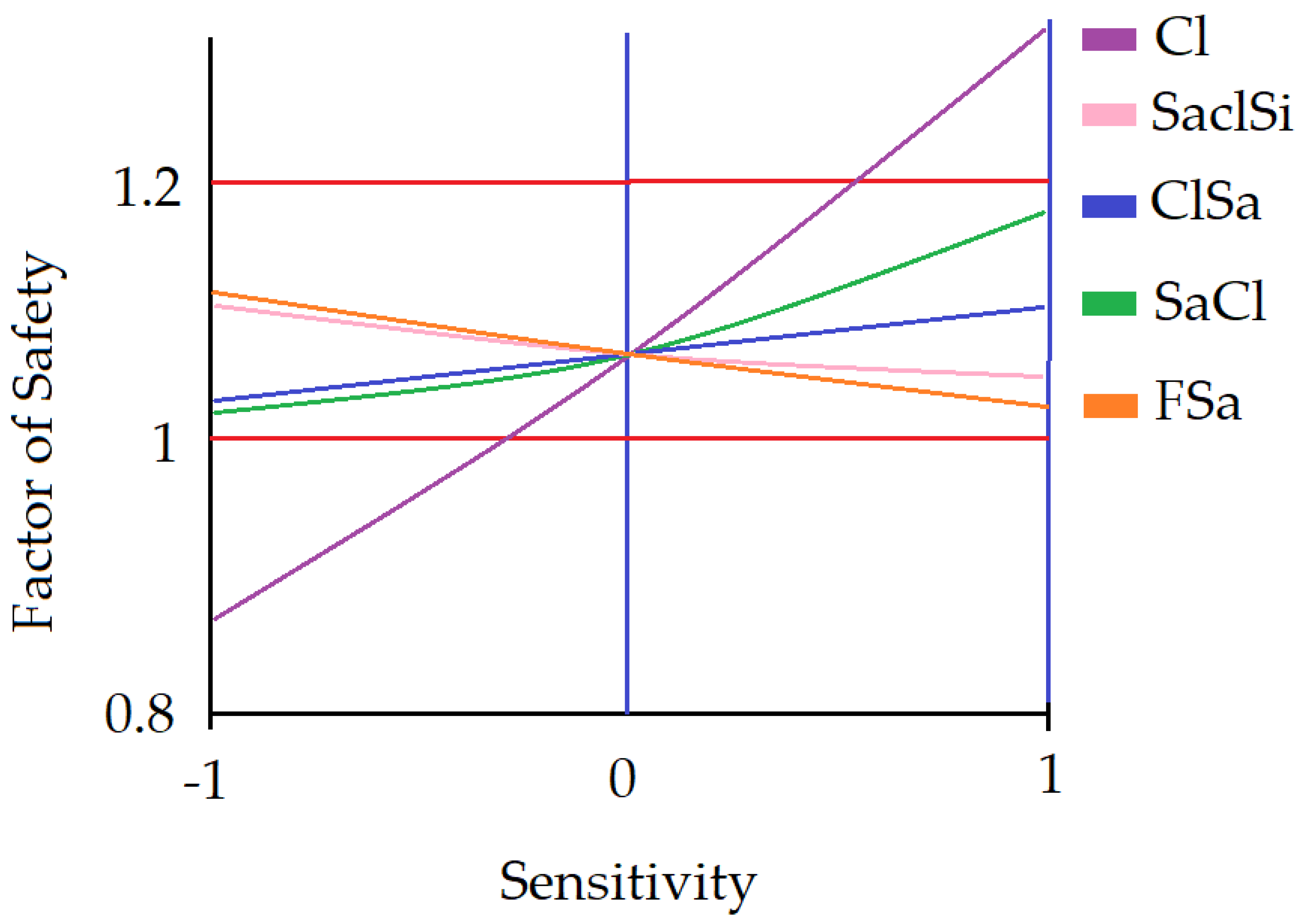
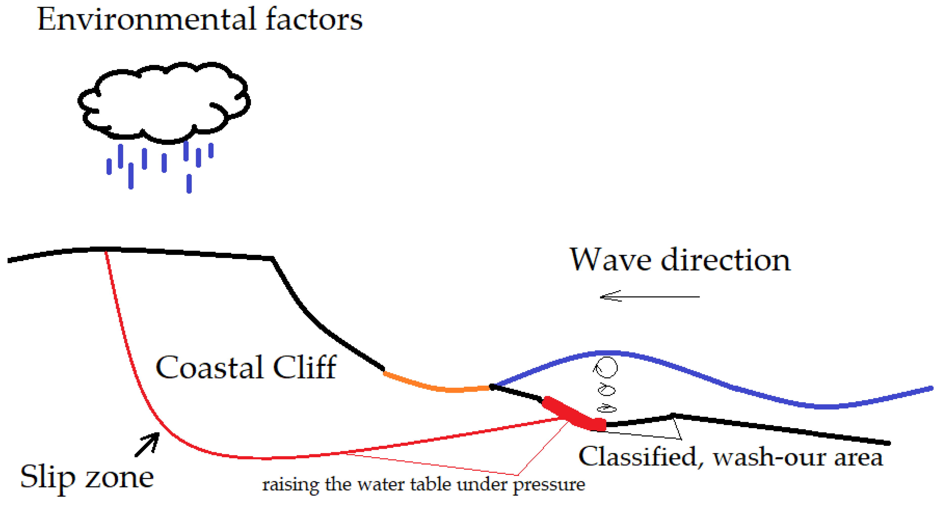
Table 1.
Measurement characteristics taken for each device.
| 1st Flight | 2nd Flight | 3rd Flight | |
|---|---|---|---|
| Device | Riegl VQ820G | Riegl VQ820G | RIEGL VQ-1560i-DW |
| Cross-section measurements | Yes | Yes | Yes |
| Atmospheric conditions | 5 | 3–4 | 3–4 |
| No. of points | >1 billion | >1 billion | >1 billion |
| Additional Aerial Photos | Yes | No | Yes |
| Additional Red Laser scanner measurements | No | No | Yes |
Table 2.
CANUPO classification between water, sediments and proper bottom in two representative datasets from the Riegl VQ820G. Each scenario shows the results from (a) the first flight and (b) the second flight.
Table 2.
CANUPO classification between water, sediments and proper bottom in two representative datasets from the Riegl VQ820G. Each scenario shows the results from (a) the first flight and (b) the second flight.
| Class Name | Total Probes | Truly Classified | Falsely Classified | Balanced Accuracy (ba) | Fisher Discriminant Ratio (fdr) |
|---|---|---|---|---|---|
| (a) Water and Sediments | 619 | 610 | 9 | 0.99 | 15.1 |
| (a) Proper Bottom | 472 | 439 | 33 | 0.93 | 6.56 |
| (b) Water and Sediments | 634 | 574 | 60 | 0.90 | 3.21 |
| (b) Proper Bottom | 607 | 599 | 8 | 0.99 | 15.1 |
Table 3.
System details for laser scanning and aerial photogrammetric devices used in the experiment.
Table 3.
System details for laser scanning and aerial photogrammetric devices used in the experiment.
| Product | Point Cloud | Point Cloud | Aerial Photographs |
|---|---|---|---|
| Device | Riegl VQ820G | RIEGL VQ-1560i-DW | RIEGL VQ-1560i-DW |
| Secchi depth | 1 | 0.7 | - |
| No. of strip lines | 22 | 13 | 13 |
| Density (pts/m2) | 102 | 81 | 231 |
| Accuracy of registration (m) | 2.5 | 2.5 | - |
| Precision of registration (cm) | 2.5 | 2.5 | - |
| Ground Sample Distance (GSD) (cm) | - | - | 10 |
| No. of tie points | 12,431 | 10,487 | 387,611 |
| Registered distance from the coastline (m) | 1000 | 500 | 300 |
| No. of measured cross-sections | 21 | 18 | 18 |
| Observed vegetation under water | No | No | No |
Table 4.
Ground control network transformation results.
| No. | Transformation Matrix | Standard Deviation (cm) |
|---|---|---|
| 1 | σ1 = 1.82 | |
| 2 | σ1 = 3.79 | |
| 3 | σ1 = 3.21 | |
| 4 | σ1 = 2.91 | |
| 5 | σ1 = 4.03 | |
| 6 | σ1 = 1.23 | |
| 7 | σ = 4.68 | |
| 8 | σ = 4.15 | |
| 9 | σ = 4.44 |
Table 5.
Geotechnical parameters used for geotechnical analysis [13].
Table 5.
Geotechnical parameters used for geotechnical analysis [13].
| Soil | γunsat (kN/m3) | γsat (kN/m3) | c’ (kPa) | (°) | E0 (MPa) | ν |
|---|---|---|---|---|---|---|
| Till (saclSi) | 20.00 | 20.13 | 30.10 | 17.50 | 23.0 | 0.27 |
| Sandy Clay (saCl) | 20.50 | 20.71 | 35.55 | 20.00 | 31.3 | 0.29 |
| Clay (Cl) | 20.00 | 20.00 | 40.00 | 21.80 | 40.0 | 0.37 |
| Clayey Sand (clSa) | 21.50 | 21.85 | 15.00 | 20.00 | 67.5 | 0.20 |
| Fine Sand (FSa) | 21.50 | 21.85 | 1.00 | 30.00 | 67.5 | 0.20 |
Publisher’s Note: MDPI stays neutral with regard to jurisdictional claims in published maps and institutional affiliations. |
© 2020 by the author. Licensee MDPI, Basel, Switzerland. This article is an open access article distributed under the terms and conditions of the Creative Commons Attribution (CC BY) license (http://creativecommons.org/licenses/by/4.0/).
Share and Cite
MDPI and ACS Style
Tysiac, P. Bringing Bathymetry LiDAR to Coastal Zone Assessment: A Case Study in the Southern Baltic. Remote Sens. 2020, 12, 3740. https://0-doi-org.brum.beds.ac.uk/10.3390/rs12223740
AMA Style
Tysiac P. Bringing Bathymetry LiDAR to Coastal Zone Assessment: A Case Study in the Southern Baltic. Remote Sensing. 2020; 12(22):3740. https://0-doi-org.brum.beds.ac.uk/10.3390/rs12223740
Chicago/Turabian StyleTysiac, Pawel. 2020. "Bringing Bathymetry LiDAR to Coastal Zone Assessment: A Case Study in the Southern Baltic" Remote Sensing 12, no. 22: 3740. https://0-doi-org.brum.beds.ac.uk/10.3390/rs12223740
Note that from the first issue of 2016, this journal uses article numbers instead of page numbers. See further details here.