FPGA-Based On-Board Hyperspectral Imaging Compression: Benchmarking Performance and Energy Efficiency against GPU Implementations

Abstract

Remote-sensing platforms, such as Unmanned Aerial Vehicles, are characterized by limited power budget and low-bandwidth downlinks. Therefore, handling hyperspectral data in this context can jeopardize the operational time of the system. FPGAs have been traditionally regarded as the most power-efficient computing platforms. However, there is little experimental evidence to support this claim, which is especially critical since the actual behavior of the solutions based on reconfigurable technology is highly dependent on the type of application. In this work, a highly optimized implementation of an FPGA accelerator of the novel HyperLCA algorithm has been developed and thoughtfully analyzed in terms of performance and power efficiency. In this regard, a modification of the aforementioned lossy compression solution has also been proposed to be efficiently executed into FPGA devices using fixed-point arithmetic. Single and multi-core versions of the reconfigurable computing platforms are compared with three GPU-based implementations of the algorithm on as many NVIDIA computing boards: Jetson Nano, Jetson TX2 and Jetson Xavier NX. Results show that the single-core version of our FPGA-based solution fulfils the real-time requirements of a real-life hyperspectral application using a mid-range Xilinx Zynq-7000 SoC chip (XC7Z020-CLG484). Performance levels of the custom hardware accelerator are above the figures obtained by the Jetson Nano and TX2 boards, and power efficiency is higher for smaller sizes of the image block to be processed. To close the performance gap between our proposal and the Jetson Xavier NX, a multi-core version is proposed. The results demonstrate that a solution based on the use of various instances of the FPGA hardware compressor core achieves similar levels of performance than the state-of-the-art GPU, with better efficiency in terms of processed frames by watt.

1. Introduction

Hyperspectral technology has experienced a steady surge in popularity in recent decades. Among the main reasons that have given hyperspectral imaging greater visibility is the richness of spectral information collected by this kind of sensor. This feature has positioned hyperspectral analysis techniques as the mainstream solution for the analysis of land areas and the identification and discrimination of visually similar surface materials. As a consequence, this technology has acquired increasing relevance, being widely used for a variety of applications, such as precision agriculture, environmental monitoring, geology, urban surveillance and homeland security, among others. Nevertheless, hyperspectral image processing is accompanied by the management of large amounts of data, which affects, on one hand, its real-time performance and, on the other hand, the requirements of the on-board storage resources. Additionally, the latest technological advances are promoting to market hyperspectral cameras with higher spectral and spatial resolutions. All of this makes the efficient data handling, from an on-board processing, communication, and storage point of view, even more challenging [1,2].

Traditionally, images sensed by spaceborne Earth-observation missions are not on-board processed. The main rationale behind this is the limited on-board power capacity that forces the use of low-power devices, which are normally not as highly performing as their commercial counterparts [3,4,5,6,7,8]. In this regard, images are subsequently downloaded to the Earth surface where they are off-line processed on high-performance computing systems based on Central Processing Units (CPUs), Graphics Processing Units (GPUs), Field-Programmable Gate Arrays (FPGAs), or heterogeneous architectures. In the case of airborne capturing platforms, images are normally on-board stored and hence the end user could not access them until the flight mission is over [9]. Additionally, unmanned aerial vehicles (UAVs) have gained momentum in recent years. They have become a very popular solution for inspection, surveillance and monitoring since they represent a lower-cost approach with a more flexible revisit time than the aforementioned Earth-observation platforms. In this context, hyperspectral image management is addressed similarly to how it is done in airborne platforms, although a lot of efforts have been made recently to transmit the images to the ground segment as soon as they are captured [10,11].

Regrettably, the data transmission from the aforementioned remote-sensing observation platforms introduces important delays. They are mainly related to the transference of large volumes of data and the limited communication bandwidths between the source and the final target, which has also kept relatively stable over the years [6,12,13]. Consequently, it reveals a bottleneck in the downlink systems that can seriously affect to the effective performance of real-time or nearly real-time applications. However, the steadily growing data-rate of the latest-generation sensors makes it compulsory to reach higher compression ratios and to carry out a real-time compression performance in order to prevent the unnecessary accumulation of high amounts of uncompressed data on-board and to facilitate efficient data transfers [14].

In this scenario of limited communication bandwidths and increasing data volumes, it is becoming necessary to move from lossless or near-lossless compression approaches to lossy compression techniques. Despite most of the state-of-the-art lossless compressors bringing a quite satisfactory rate-distortion performance, the former approaches provide very moderate compression ratios of about 2∼3:1 [15,16], which presently are not sufficient to handle the high input data-rate of the newest-generation sensors. For this reason, a research effort targeting lossy compression is currently being made [17,18,19,20,21]. Due to the limited on-board computational capabilities of remote-sensing hyperspectral acquisition systems, low-complexity compression schemes stand as the most practical solution for such restricted environments [21,22,23,24]. Nevertheless, most of the state-of-the-art lossy compressors are generalizations of existing 2D images or video compression algorithms [25]. For this reason, they are normally characterized by high computational burden, intensive memory requirements and a non-scalable nature. These features prevent their use in power-constrained applications with limited hardware resources, such as on-board compression [26,27].

In this context, the Lossy Compression Algorithm for Hyperspectral Image Systems (HyperLCA) [28] was developed as a novel hardware-friendly lossy compressor for hyperspectral images. HyperLCA was introduced as a low-complexity alternative that provides a good compression performance at high compression ratios with a reasonable computational burden. Additionally, this algorithm permits compressing blocks of image pixels independently which promotes, on the one hand, the reduction of the data to be managed at once besides the hardware resources to be allocated. On the other hand, the HyperLCA algorithm becomes a very competitive solution for most applications based on pushbroom/whiskbroom scanners, paving the way for real-time compression performance. The flexibility and the high level of parallelism intrinsic to the HyperLCA algorithm has been previously evaluated in earlier publications. In particular, its suitability for real-time performance in applications characterized by high data-rates with restrictions in computational resources due to power, weight or space was tested in [29].

In this work, we focus on a use case where a visible-near-infrared (VNIR) hyperspectral pushbroom scanner is mounted onto a UAV. In particular, we have analyzed the performance of FPGAs for the lossy compression of hyperspectral images against low-power GPUs (LPGPUs) in order to establish the benefits and barriers of using each one of these hardware devices for the on-board compression task. Specifically, we have implemented the HyperLCA algorithm in a Xilinx Zynq-7000 programmable System on Chip (SoC). We have selected this SoC because it can be found in low-cost, low-weight and compact-size development boards, such as MicroZed^TM and PYNQ boards. Although UAVs have been consolidated as trending aerial observation platforms, their acquisition costs are still not accessible for many end customers, not only those who want to purchase them but also those who lease their services. For this reason, we must also aim to solve the economic implications that comes along with these devices. On this basis, in this work we have focused on the on-board computing platform, searching for a less expensive alternative that, in exchange, cannot offer the same level of both performance and functionality than other costly commercial products. Additionally, it is important to note that while experiments carried out in this work are oriented to the current necessities imposed by an application based on drones, all drawn conclusions can be extrapolated to other fields in which remotely sensed hyperspectral images have to be compressed in real time, such as spaceborne missions that employs next-generation space-grade FPGAs.

The rest of this paper is organized as follows. Section 2 gives outlines of the majority issues around the operations involved in the HyperLCA algorithm. In addition, it also includes a detailed explanation about the implementation model developed for the execution of the HyperLCA compressor on the selected FPGA SoC. Section 3 analyzes the obtained experimental results in terms of both quality of the compression process and hardware implementation points of view. Section 4 discusses the strengths and limitations of the proposed solution and includes a comparison evaluation of the obtained results with those achieved by a selection of LPGPUs embedded systems, following the implementation model shown in [29]. Finally, Section 5 draws the main conclusions of this work.

2. Materials and Methods

2.1. HyperLCA Algorithm

The HyperLCA algorithm is a novel lossy compressor for hyperspectral images especially designed for applications based on pushbroom/whiskbroom sensors. Concretely, this transform-based solution can independently compress blocks of image pixels regardless of any spatial alignment between pixels. Consequently, it facilitates the parallelization of the entire compression process and makes it relatively simple to stream the compression of hyperspectral frames collected by a pushbroom or whiskbroom sensor. Additionally, the HyperLCA compressor also allows fixing a desired minimal compression ratio and guaranties that at least this minimum will be achieved for each block of image pixels. This makes it possible to know in advance the maximum data rate that will be attained after the acquisition and compression processes in order to efficiently manage the data transfers and/or storage. Additionally, the HyperLCA compressor provides quite satisfactory rate-distortion results for higher compression ratios than those achievable by lossless compression approaches. Furthermore, the HyperLCA algorithm preserves the most characteristic spectral features of image pixels that are potentially more useful for ulterior hyperspectral analysis techniques, such as target detection, spectral unmixing, change detection, anomaly detection, among others [30,31,32,33,34].

Figure 1 shows a graphic representation of the main computing stages involved by the HyperLCA compressor. First, the Initialization stage configures the same parameters ($p_{max}$) employing the input parameters $CR$, $N_{bits}$ and $BS$. Since the HyperLCA compressor follows an unmixing-like strategy, the $p_{max}$ most representative pixels within a block of image pixels to be independently processed are compressed with the highest precision. Then, other image pixels are reconstructed using their scalar projections, V, over the previously selected pixels. Therefore, $p_{max}$ is estimated according to the minimum desired compression ratio to be reached, $CR$, the number of hyperspectral pixels within each image block, $BS$ and the number of bits used for representing the values of V vectors. Second, these $p_{max}$ characteristic pixels are selected using orthogonal projection techniques in the HyperLCA Transform stage. It results in a spectral uncorrelated version of the original hyperspectral data. Thirdly, the outputs of the HyperLCA Transform stage are adapted in the following HyperLCA Preprocessing stage for being later more efficiently codified in the fourth and last HyperLCA Entropy Coding stage. In the following lines, the operations involved in these four algorithm stages are further analyzed in order to give a glance of the decisions taken for the acceleration of the HyperLCA algorithm in hardware devices based on FPGAs.

2.1.1. General Notation

Before starting the algorithm description, it is necessary to introduce the general notation followed thorough the rest of this manuscript. In this sense, $\mathbf{HI}=\left\{{\mathbf{F}}_i,i=1,...,nr\right\}$ is a sequence of $nr$ scanned cross-track lines of pixels acquired by a pushbroom sensor, ${\mathbf{F}}_i$, comprised by $nc$ pixels with $nb$ spectral bands. Pixels within $\mathbf{HI}$ are grouped in blocks of $BS$ pixels, ${\mathbf{M}}_k=\left\{{\mathbf{r}}_j,j=1,...,BS\right\}$, being normally $BS$ equal to $nc$, or multiple of it, and k spans from 1 to $\frac{nr·nc}{BS}$. $\widehat{\mathbf{\mu }}$ represents the average pixel of each image block, ${\mathbf{M}}_k$. Therefore, C is defined as the centralized version of ${\mathbf{M}}_k$ after being subtracted $\widehat{\mathbf{\mu }}$ from all image pixels. $\mathbf{E}=\left\{{\mathbf{e}}_n,n=1,...,p_{\max }\right\}$ saves the $p_{\max }$ most different hyperspectral pixels extracted from each ${\mathbf{M}}_k$ block. $\mathbf{V}=\left\{{\mathbf{v}}_n,n=1,...,p_{\max }\right\}$ comprises $p_{\max }$ vectors of $BS$ elements where each ${\mathbf{v}}_n$ vector corresponds to the projection of the $BS$ pixels within ${\mathbf{M}}_k$ onto the corresponding n extracted pixel, ${\mathbf{e}}_n$. $\mathbf{Q}=\left\{{\mathbf{q}}_n,n=1,...,p_{\max }\right\}$ and $\mathbf{U}=\left\{{\mathbf{u}}_n,n=1,...,p_{\max }\right\}$ save $p_{\max }$ pixels of $nb$ bands that are orthogonal among them.

2.1.2. HyperLCA Initialization

The HyperLCA compressor must first determine the number of pixels, ${\mathbf{e}}_n$, and projection vectors, ${\mathbf{v}}_n$, ($p_{\max }$) to be extracted from each image block, ${\mathbf{M}}_k$, according to the input parameters $CR$, $N_{bits}$ and $BS$, as shown in Equation (1). In it, DR refers to the number of bits per pixel per band used for representing the hyperspectral image elements to be compressed. As can be deduced, the number of selected pixels, $p_{\max }$, directly determines the maximum compression ratio to be reached with the selected algorithm configuration. Furthermore, bigger $p_{\max }$ results in better reconstructed images but lower compression ratios.

$$p_{\max }\le \frac{DR·nb·(BS-CR)}{CR·(DR·nb+N_{\mathrm{bits}}·BS)}$$

(1)

2.1.3. HyperLCA Transform

The HyperLCA compressor is a transform-based algorithm that employs a modified version of the well-known Gram-Schmidt orthogonalization method to obtain a compressed and uncorrelated image. In this regard, the HyperLCA Transform stage oversees carrying out the spectral transform. For this reason, it is the algorithm stage that involves the most demanding computing operations and thus, which are more prone to be accelerated in parallel dedicated hardware devices.

The HyperLCA Transform is described in detail in Algorithm 1. As can be seen, the HyperLCA Transform stage receives as inputs the hyperspectral image block to be compressed, ${\mathbf{M}}_k$, and the number of hyperspectral pixels to be extracted, $p_{\max }$. As outputs, the HyperLCA Transform states the set of the $p_{\max }$ most different hyperspectral pixels, $\mathbf{E}$, and their corresponding projection vectors, $\mathbf{V}$. For doing so, the hyperspectral image block, ${\mathbf{M}}_k$, is first centralized by subtracting the average pixel, $\widehat{\mathbf{\mu }}$, from all pixels within ${\mathbf{M}}_k$, which results in the centralized version of the data, $\mathbf{C}$, in line 3. Second, the $p_{\max }$ most characteristic pixels are sequentially extracted from lines 4 to 15. In this iterative process, the brightness of each image pixel is calculated in lines 5 to 7. It is defined as the dot product of each image pixel with itself (see line 6). The extracted pixels, ${\mathbf{e}}_n$, are those pixels within the original image block, ${\mathbf{M}}_k$, with the highest brightness in each iteration, n (see line 8 and 9). Afterwards, the orthogonal vectors ${\mathbf{q}}_n$ and ${\mathbf{u}}_n$ are accordingly defined as shown in lines 10 and 11, respectively. ${\mathbf{u}}_n$ is employed to estimate the projection of each image pixel over the direction spanned by the selected pixel, ${\mathbf{e}}_n$, deriving in the projection vector, ${\mathbf{v}}_n$ in line 12. Finally, this information is subtracted from $\mathbf{C}$ in line 13.

Accordingly, $\mathbf{C}$ retains in next iterations the spectral information that cannot be represented by the already selected pixels ${\mathbf{e}}_n$. For this reason, once the $p_{\max }$ pixels have been extracted, $\mathbf{C}$ contains the spectral information that will be not recovered after the decompression process. Hence, it is represented of the losses introduced by the HyperLCA compressor. Consequently, the remaining information in $\mathbf{C}$ could be used to establish extra stopping conditions based on quality metrics, such as the Signal-to-Noise Ratio (SNR) or the Maximum Absolute Difference (MAD). In this work, these extra stopping conditions have been discarded, and thus, a fixed number of $p_{\max }$ iterations is executed for all image blocks, ${\mathbf{M}}_k$.

Algorithm 1 HyperLCA Transform.

Inputs:

${\mathbf{M}}_k=[{\mathbf{r}}_1,{\mathbf{r}}_2,...,{\mathbf{r}}_{BS}]$, $p_{max}$

Outputs:

$\widehat{\mathbf{\mu }}$; $\widehat{\mathbf{\mu }}$; $\mathbf{E}=[{\mathbf{e}}_1,{\mathbf{e}}_2,...,{\mathbf{e}}_{p_{max}}]$; $\mathbf{V}=[{\mathbf{v}}_1,{\mathbf{v}}_2,...,{\mathbf{v}}_{p_{max}}]$

Algorithm:

1:  {Additional stopping condition initialization.}

2:  Average pixel: $\widehat{\mathbf{\mu }}$;

3:  Centralized image: $\mathbf{C}={\mathbf{M}}_k-\widehat{\mathbf{\mu }}=[{\mathbf{c}}_1,{\mathbf{c}}_2,...{\mathbf{c}}_{BS}]$;

4:  for  $n=1$  to  $p_{max}$  do

5:        for $j=1$  to  $BS$ do

6:        Brightness Calculation: ${\mathbf{b}}_j={\mathbf{c}}_j^{\prime }·{\mathbf{c}}_j$;

7:         end for

8:     Maximum Brightness: $j_{max}=$ argmax(${\mathbf{b}}_j$);

9:     Extracted pixels: ${\mathbf{e}}_n={\mathbf{r}}_{j_{max}}$;

10:     ${\mathbf{q}}_n={\mathbf{c}}_{j_{max}}$;

11:     ${\mathbf{u}}_n={\mathbf{q}}_n/b_{j_{max}}$;

12:     Projection vector: ${\mathbf{v}}_n={\mathbf{u}}_n^{\prime }·\mathbf{C}$;

13:     Information Subtraction: $\mathbf{C}=\mathbf{C}-{\mathbf{q}}_n·{\mathbf{v}}_n$;

14:     {Additional stopping condition checking.}

15:  end for

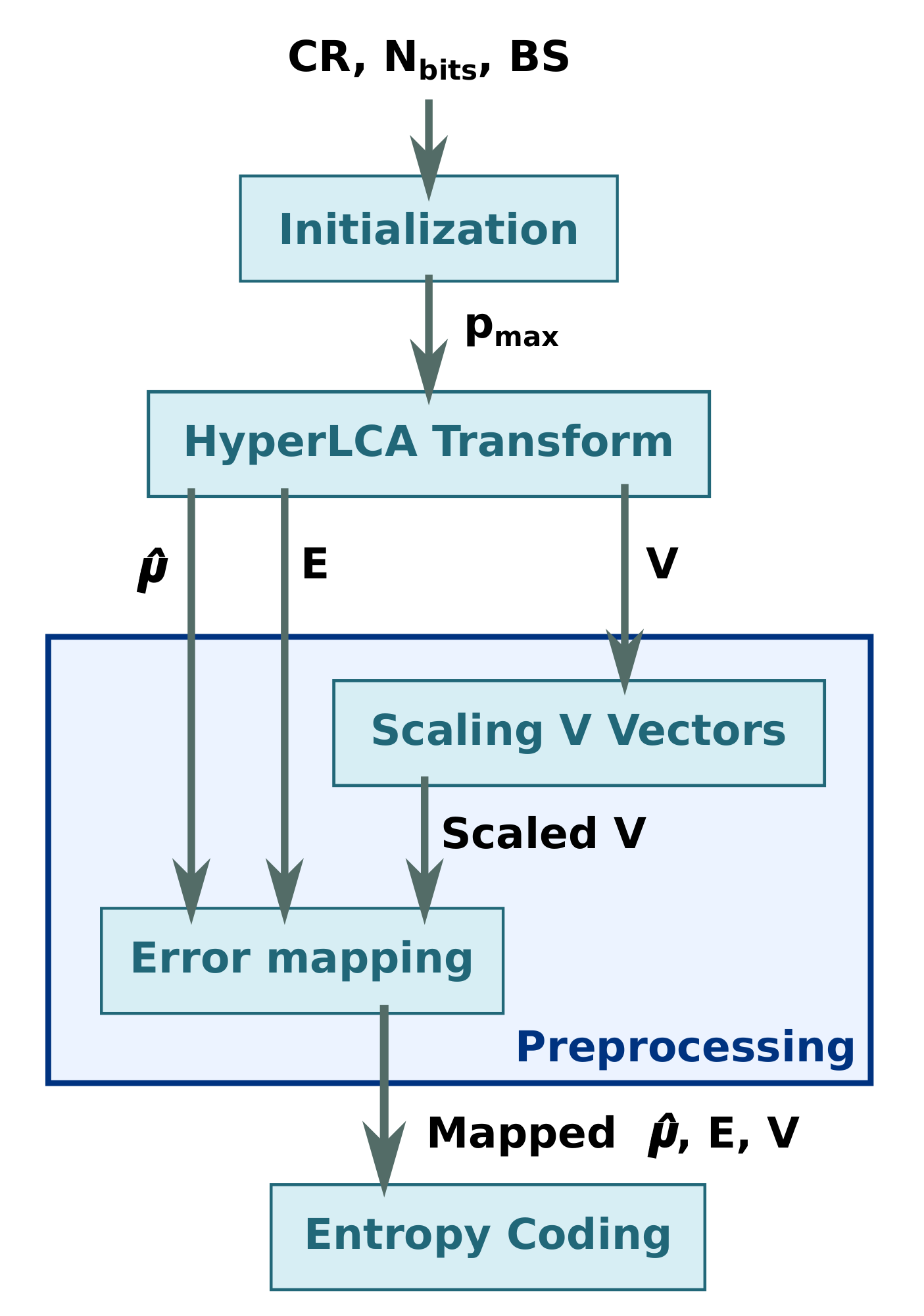
2.1.4. HyperLCA Preprocessing

To ensure an efficient entropy coding of the HyperLCA Transform outputs, they must be first adapted in the HyperLCA Preprocessing stage. This transformation process is performed in two steps:

Scaling V Vectors

$\mathbf{V}$ vectors represent the projection of each pixel within ${\mathbf{M}}_k$ over the direction spanned by each orthogonal vector, ${\mathbf{u}}_n$, in each iteration. Therefore, potential values of each element of $\mathbf{V}$ vectors are in the range of $\left(-1,1\right]$. However, the later Entropy-coding stage works exclusively with integers. Consequently, elements within $\mathbf{V}$ must be scaled to fully exploit the dynamic range offered by the input parameter $N_{\mathrm{bits}}$, as shown in Equation (2). After doing so, the scaled $\mathbf{V}$vectors are rounded up to the closest integer values.

$$v_{j_{\mathrm{scaled}}}=(v_j+1)·(2^{N_{\mathrm{bits}}-1}-1)$$

(2)

Error Mapping

The codification stage also exploits the redundancies within the data in the spectral domain to assign the shortest word length to the most common values. With it, the compression ratio achieved by the HyperLCA Transform could be even increased. To this end, the output vectors of the HyperLCA Transform ($\widehat{\mathbf{\mu }}$, E and scaled V) are lossless pre-processed in the Error Mapping stage. To do so, the prediction error mapper described in the Consultative Committee for Space Data Systems (CCSDS) Blue Books is employed [35]. In this regard, each output vector, ($\widehat{\mathbf{\mu }}$, ${\mathbf{e}}_n$ and scaled ${\mathbf{v}}_n$) is individually processed and transformed to be exclusively composed of positive integer values closer to zero.

2.1.5. HyperLCA Entropy Coding

The Entropy Coding is the last stage of the HyperLCA compressor. It follows a lossless entropy-coding strategy based on the Golomb–Rice algorithm [36]. As in the Error Mapping stage, each single output vector is independently coded. For doing so, the compression parameter, M, is estimated as the average value of the targeted vector. Afterwards, each of its elements is divided by M in order to obtain the results of the division, the quotient (q) and the remainder (r). On one hand, the quotient, q, is codified using unary code. On the other hand, the remainder, r, could be coded using $b=lo{g}_2\left(M\right)+1$ bits if M is power of 2. Nevertheless, M can actually be any positive integer. For this reason, the remainder, r is coded as plain binary using $b-1$ bits for r values smaller than $2^b-M$, otherwise it is coded as $r+2^b-M$ using b bits.

2.1.6. HyperLCA Data Types and Precision Evaluation

Most of the compression performance achieved by the HyperLCA algorithm is obtained in the HyperLCA Transform stage, originally designed to use floating-point precision. However, FPGA devices are, in general, more efficient dealing with integer operations. Additionally, the execution of floating-point operations in different devices may produce slightly different results. For this reason, the performance of the HyperLCA algorithm using integer arithmetic was largely drawn in [37] in order to adapt it for being more suitable for this kind of device. In particular, it was used the fixed-point concept in a custom way employing integer arithmetic and bits shifting [38]. In this previous work, two different versions of the HyperLCA Transform were considered employing 32 and 16 bits, respectively, for representing the image values stored in the centralized version of the hyperspectral frame to be processed, C.

It is important to note that the aforementioned proposed versions were developed for working with hyperspectral images whose element values could be represented with up to 16 bits per pixel per band as maximum. In this context, the quality of the compression results is very similar between the 32-bits fixed point and the single precision floating-point versions. Nevertheless, the compression performance obtained by the 16-bit version is not as competitive as the other two solutions. It is shown that this 16-bit approach provides its best performance for very high compression ratios, small $BS$ and images packaged using less than 16 bits per pixel per band. This makes the 16-bits version into a very interesting option for applications with limited hardware resources, especially the availability of in-chip memory, one of the weaknesses of FPGAs.

On this basis, we have made some performance-enhancing improvements to the 16-bit version to obtain better compression results. In this context, we have assumed that the available capturing system codes hyperspectral images with a maximum of 12 bits, which is also the most common scenario in remote-sensing applications [39,40] and in the one outlined in this manuscript.

Table 1. Number of bits used for the integer and decimal parts used to represent the variables involved in the HyperLCA Transform. Three versions of the algorithm were developed to use integer arithmetic (I32, I16, I12).

Variable	Integer Part			Decimal Part			Total
		I32	I16	I12	I32	I16	I12	I32	I16	I12
C	20	16	14	12	0	2	32	16	16
b	48	48	48	16	16	16	64	64	64
q	20	20	20	12	12	12	32	32	32
u	2	2	2	30	30	30	32	32	32
v	2	2	2	30	30	30	32	32	32
$\mathbf{\mu }$	16	16	12	0	0	0	16	16	12

summarizes the number of bits used by the two algorithm versions introduced in [37], known as I32 and I16, and the one described in this work, referred as to I12, for some algorithm variables. It should be pointed out that when integer arithmetic is used, V vectors are directly represented using integer data types and do not need to be scaled and rounded to integer values.

As described in Section 2.1.3, the information presents in matrix C decreases with every iteration, n, though some specific values may increase in some quite unlikely situations. For this reason, initial values of C were divided by 2 in the previous 16-bit version in order to avoid overflowing, what directly decreases the precision in one bit. In the new version proposed in this work, this fact is discarded since we have 2 bits extra for these improbable situations. As can be noticed from Table 1, image C is stored employing 16 bits in the new I12 version as well as in the I16 version. However, it is assumed that images values are coded employing 12 bits as maximum instead of 16 bits. It permits having 2 extra bits for representing the integer part of the fixed-point values of C elements. Consequently, image precision is not altered as in previous 16-bit version for dealing with possible overflowing scenarios. Additionally, this new version also allows having 2 bits for representing the decimal part of the fixed-point values of matrix C, which is not possible in the I16 version.

2.2. FPGA Implementation of the HyperLCA Algorithm

An FPGA (Field-Programmable Gate Array) can be seen as a whiteboard for designing specialized hardware accelerators (HWacc), by composition of predefined memory and logic blocks that are available in the platform. Therefore, a HWacc is a set of architectural FPGA resources, connected and configured to carry out a specific task. Each vendor proposes its own reconfigurable platform, instantiating a particular mix of such resources, around a particular interconnection architecture.

FPGAs provide flexibility to designers, since the silicon adapts to the solution, instead of fitting the solution to the computing platform as is the case of GPU-based solutions. On top of that, FPGA-based implementations can take advantage of the fine-grain parallelism of their architecture (operation level) as well as task-level concurrency. In this paper, the HyperLCA lossy compressor has been implemented onto a heterogeneous Zynq-7000 SoC (System-on-a-Chip) from Xilinx that combines a Processor System (PS), based on a dual core ARM processor, and a Programmable Logic (PL), based on a Artix-7/Kintex-7 FPGA architecture.

The development process followed a productive methodology based on High-Level Synthesis (HLS). This methodology focuses the effort on the design and verification of the HWacc, as well as the exploration of the solution space that helps to speed up the search for value-added solutions. The starting point of a methodology based on HLS is a high-abstraction model of the functionality to be deployed on the FPGA, usually described by means of high-level programming languages, such as C or C++. Then, HLS tools can generate the corresponding RTL (Register Transfer Level) implementation, functionally equivalent to the C or C++ model [41,42].

Productivity is the strongest point of HLS technology, and one of the main reasons why hardware architects and engineers have been recently attracted to it. However, HLS technology (more specifically, the tools that implement the synthesis process) has some weaknesses. For example, despite the fact that the designer can describe a modular and hierarchical implementation of a HWacc (i.e., grouping behavior via functions or procedures), all sub-modules are orchestrated by a global clock due to the way the translation to RTL from C is done. Another example is the rigid semantic when specifying dataflow architectures, allowing a reduced number of alternatives. This prevents the designer from obtaining optimal solutions for certain algorithms and problems [43,44], as was the case of the HyperLCA compressor. Therefore, to overcome the limitations of current HLS tools, a hybrid solution that combines modules developed using VHDL and HLS-synthesized C or C++ blocks has been selected. The result allows the achievement of the maximum performance. Otherwise, it could not be possible to realize either the synchronization mechanisms or the parallel processing proposed in this work. On top of that, this approach makes it also possible to optimize the necessary resources because of the use of custom producer-consumer data exchange patterns that are not supported by HLS tools.

The four main stages of the HyperLCA compressor, described in Section 2.1 and shown in Figure 1, have been restructured in order to better adapt to devices with a high degree of fine-grain parallelism such as FPGAs. Thus, the operations involved in these parts of the HyperLCA algorithm have been grouped in two main stages: HyperLCA Transform and HyperLCA Coder. These new stages can run in parallel, which improves the performance.

The Initialization stage (Section 2.1.2), where the calculation of the $p_{max}$ parameter is done, is considered only at design time. This is because several hardware components, such as internal memories or FIFOs, must be configured with the appropriate size. In this sense, it is worth mentioning that the $p_{max}$ value (Equation (1)) depends on other parameters also known at design time (the minimum desired compression ratio ($CR$), block size ($BS$) and the number of bits ($N_{bits}$) used for scaling the projection vectors, V, and, therefore, can be fixed for the HWacc.

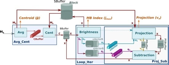
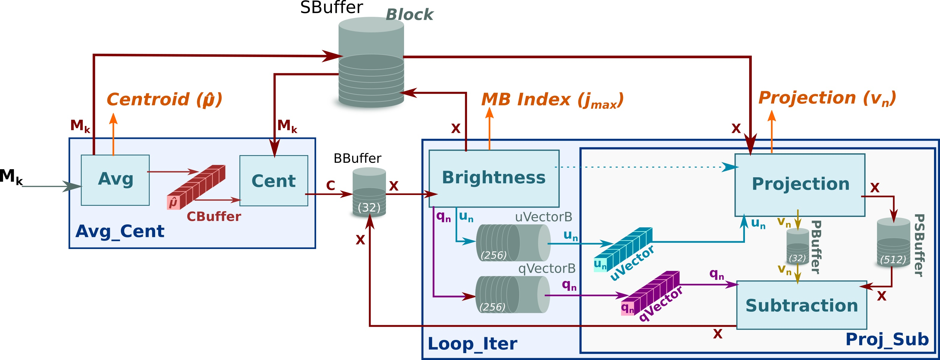
2.2.1. HyperLCA Transform

HyperLCA Transform stage performs the operations of the HyperLCA transform itself (described in Section 2.1.3), and also the computation of the average pixel and the scaling of $\mathbf{V}$ vector. These are the most computational demanding operations of the algorithm and, together with the fact that they are highly parallelizable by nature, are good candidates for acceleration.

Figure 2 shows an overview of the hardware implementation of the HyperLCA Transform stage. Avg_Cent, Brightness and Proj_Sub modules have been modeled and implemented using the aforementioned HLS tools, while the memory buffers and custom logic that integrates and orchestrates all the components in the design have been instantiated and implemented using VHDL language, respectively. This HWacc has a single entry corresponding to a hyperspectral block (${\mathbf{M}}_k$) that will be compressed, while the output is composed of three elements (which differs to the output of Algorithm 1) in order to achieve a high level of parallelism. It must also be mentioned that the output of the HyperLCA Transform stage feeds the input of the HyperLCA Coder stage that performs the error mapping and entropy coding in parallel. Thus, the centroid, $\widehat{\mathbf{\mu }}$, is obtained as depicted in Algorithm 1, while the $p_{max}$ most different hyperspectral pixels, $\mathbf{E}$, are not directly obtained. In this regard, the HWacc provides the indexes of such pixels, $j_{max}$, in each loop iteration of Algorithm 1 (outer loop), while the HyperLCA Coder is the responsible to obtaining each hyperspectral pixel, ${\mathbf{e}}_n$, from the external memory, in which is stored the hyperspectral image, to build the vector of most different hyperspectral pixels, $\mathbf{E}$. Finally, the projection of pixels within each image block, $\mathbf{V}$, is provided by the HWacc in a batch mode, i.e., each loop iteration (outer loop of Algorithm 1) obtains a projection ($v_n$) that forms part of the $\mathbf{V}$ vector.

The architecture of the HLCA Transform HWacc can be divided into two main modules: Avg_Cent, which corresponds to lines 2 and 3 of Algorithm 1, and Loop_Iter (the main loop body, lines from 5 to 14). These modules are connected by a bridge buffer (BBuffer), whose depth is only 32 words, and also share a larger buffer (SBuffer) with capacity to store a complete hyperspectral block. The size of the SBuffer depends on the BS algorithm parameter and its depth is determined at design time. The role of this SBuffer is to avoid the costly access to external memory, such it is the case of double data rate (DDR) memory in the Zynq-7000 SoCs.

The implementation of the SBuffer is based on a first-in, first-out (FIFO) memory that is written and read by different producers (i.e., Avg and Brightness) and consumers (i.e., Cent and Projection) of the original hyperspectral block and the intermediate results (transformations). Since there are more than one producer and consumer for the SBuffer, a dedicated synchronization and control access logic has been developed in VHDL (not illustrated in Figure 2). The use of a FIFO contributes to reduce the on-chip memory resources in the FPGA fabric, being its use feasible because of the linear pattern access of the producers and consumers. However, this type of solution would not have been possible with HLS because the semantic of stream-based communication between stages in a dataflow limits the number of producers and consumer to one. Also, it is not possible, with the used HLS technology, to exploit inter-loop parallelism as is done in the proposed solution. Notice that there is a data dependency between iterations in Algorithm 1 (centralized block, $\mathbf{C}$) and, therefore, the HLS tool infers that the next iteration must wait for the previous one to finish, resulting in fact in sequential computation. However, a deeper analysis of the behavior of the algorithm shows that the computation of the brightest pixel for iteration $n+1$ can be performed as it has received the output of the subtraction stage, which will be still processing iteration n.

The Avg_Cent module has been developed using HLS technology and contains two sub-modules, Avg and Cent, that implement lines 2 and 3 of Algorithm 1, respectively.

Avg 

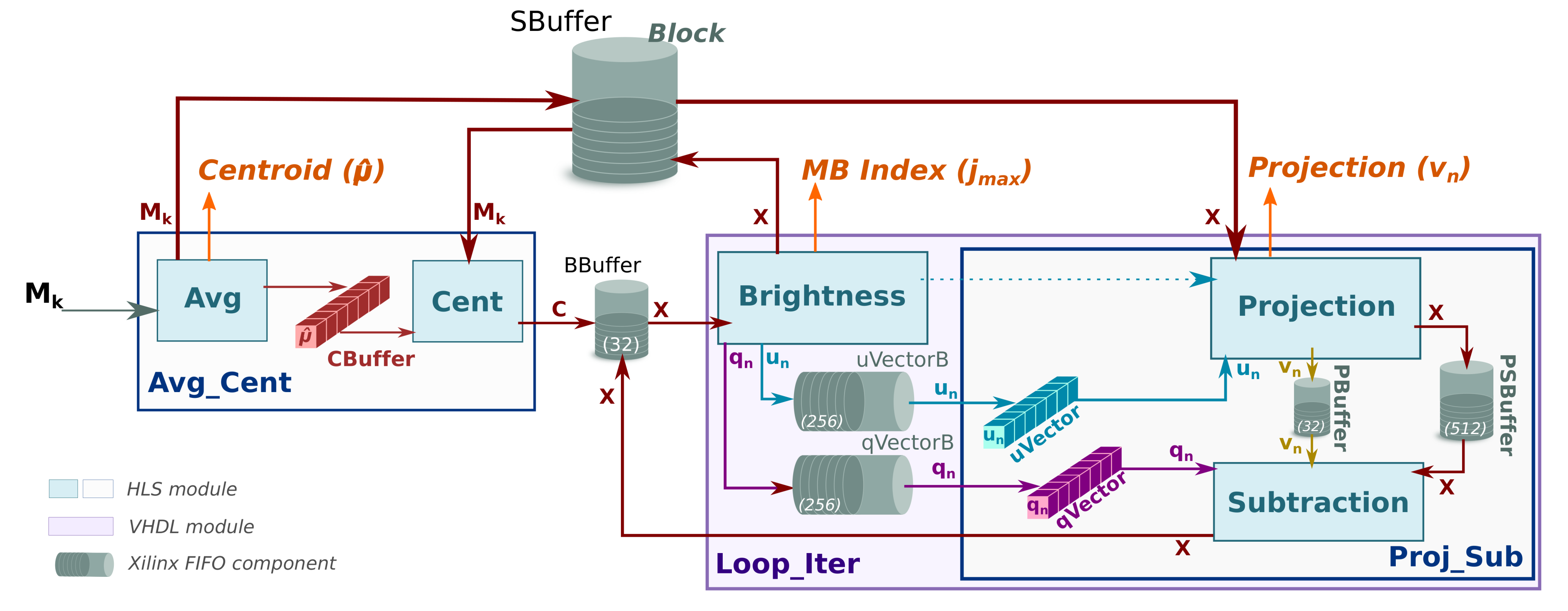
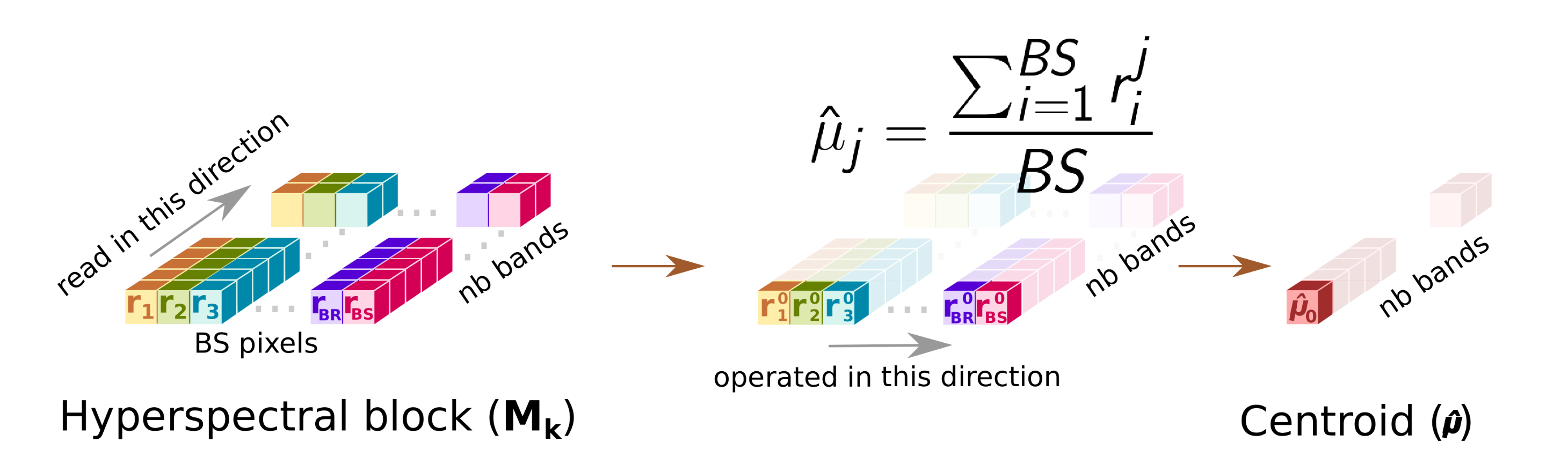
This sub-module computes the centroid or average pixel, $\widehat{\mathbf{\mu }}$, of the original hyperspectral block, ${\mathbf{M}}_k$, following line 2 of Algorithm 1, and stores it in CBuffer, a buffer that shares with Cent sub-module. During this operation, Avg forwards a copy of the centroid to the HyperLCA Coder via a dedicated port (orange arrow). At the same time, the Avg sub-module writes all the pixels of the ${\mathbf{M}}_k$ into the SBuffer. A copy of the original hyperspectral block, ${\mathbf{M}}_k$, will be available once Avg finishes, ready to be consumed as a stream by Cent, which reduces the latency.

Figure 3 shows in detail the functioning of the Avg stage. The main problem in this stage is the way the hyperspectral data is stored. In our case, the hyperspectral block, ${\mathbf{M}}_k$, is ordered by the bands that make up a hyperspectral pixel. However, to obtain the centroid, $\widehat{\mathbf{\mu }}$, the hyperspectral block must be read by bands (in-width reading) instead of by pixels (in-depth reading). We introduce an optimization that handles the data as it is received (in-depth), avoiding the reordering of the data to maintain a stream-like processing. This optimization consists of an accumulate vector, whose depth is equal to the number of bands that stores partial results of the summation for each band, i.e., the first position of this vector contains the partial results of the first band, the second position the partial results of the second band and so on. The use of this vector removes the loop-carry dependency in the HLS loop that models the behavior of the Avg sub-module, saving processing cycles. The increase in resources is minimal, which is justified by the gain in performance.

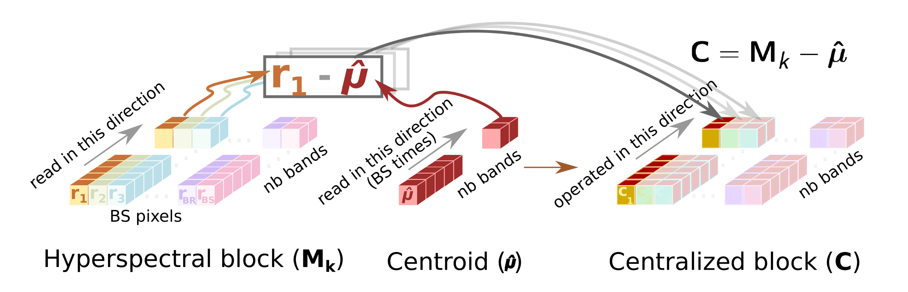
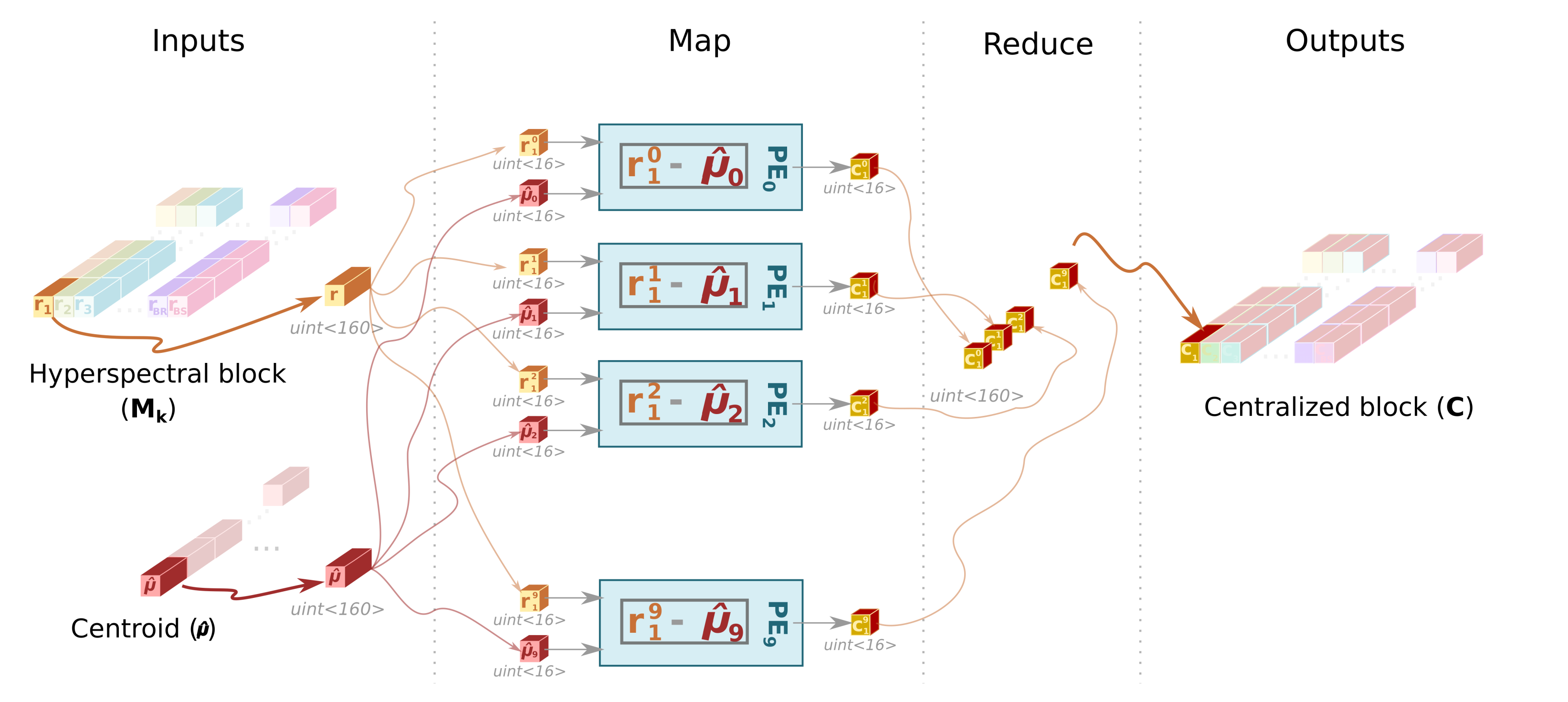
Cent 

This sub-module reads the original hyperspectral block, ${\mathbf{M}}_k$, from the SBuffer to centralize it ($\mathbf{C}$). This operation consists of subtracting the average pixel, calculated in the previous stage, from each hyperspectral pixel of the block (line 3 of Algorithm 1). Figure 4 shows this process, highlighting the elements that are involved in the centralization of the first hyperspectral pixel. Thus, the Cent block reads the centroid, $\widehat{\mathbf{\mu }}$, which is stored in the CBuffer, as many times hyperspectral pixels have the original block (i.e., $BS$ times in the example illustrated in Figure 4). Therefore, CBuffer is an addressable buffer that permanently stores the centroid of the current hyperspectral block that is being processed. The result of this stage is written into the BBuffer FIFO, which makes unnecessary an additional copy of the centralized image, $\mathbf{C}$. As soon as the centralized components of the hyperspectral pixels are computed, the data is ready at the input of the Loop_Iter module and, therefore, it can start to perform its operations without waiting for the block to be completely centralized.

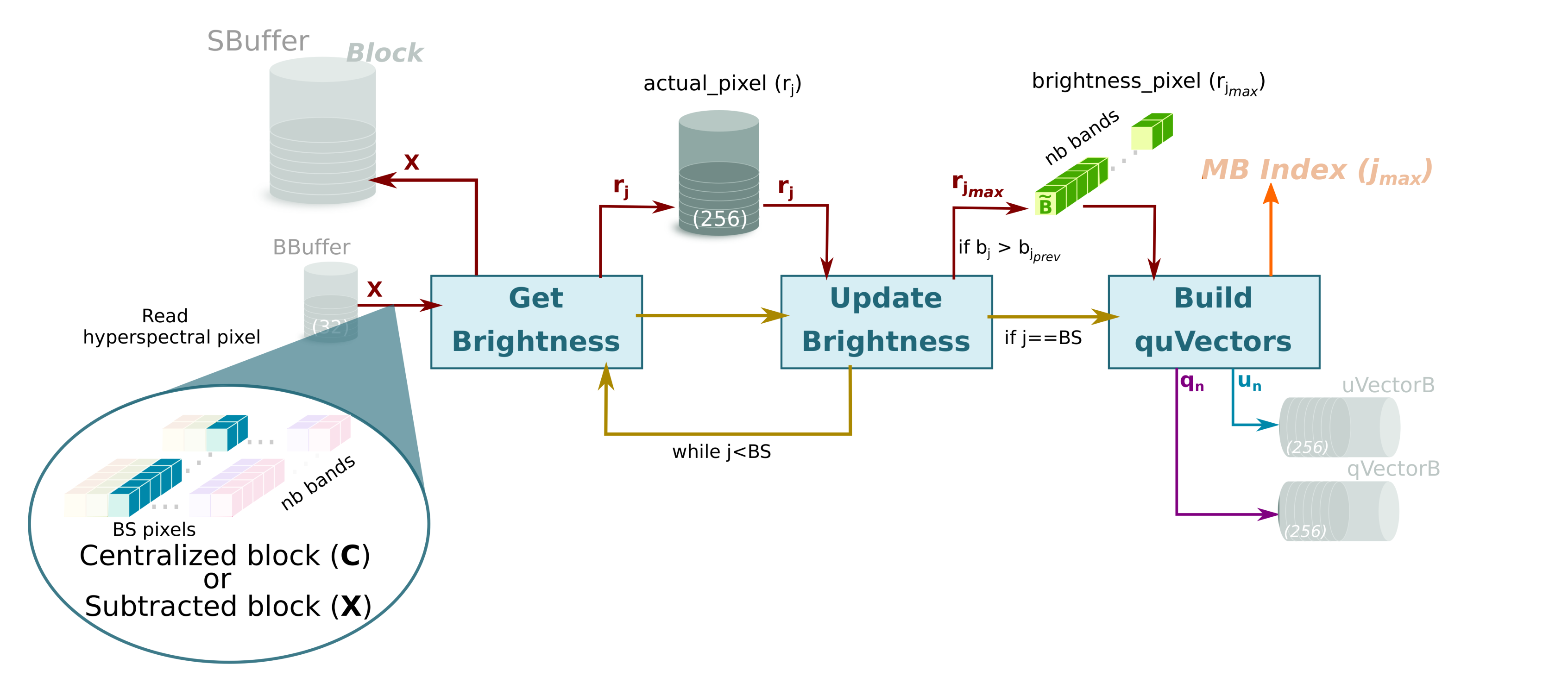
The Loop_Iter module instantiates the Brightness and Proj_Sub sub-modules which have been designed and implemented using HLS technology. Both modules are connected by two FIFO components (uVectorB and qVectorB) using customized VHDL code to link them. Unlike Avg_Cent module, Loop_Iter module is executed several times (specifically $p_{max}$ times, line 4 of Algorithm 1) for each hyperspectral block that is being processed.

Brightness 

This sub-module starts as soon as there is data in the BBuffer. In this sense, Brightness sub-module works in parallel with the rest of the system; the input of the Brightness module is the output of Cent module in the first iteration, i.e., the centralized image, $\mathbf{C}$, while the input for all other iterations is the output of Subtraction sub-module that corresponds to the image for being subtracted, depicted as $\mathbf{X}$ for the sake of clarity (see brown arrows in Figure 2).

Brightness sub-module has been optimized to achieve a dataflow behavior that takes the same time regardless of the location of the brightest hyperspectral pixel. Figure 5 shows how the orthogonal projection vectors ${\mathbf{q}}_n$ and ${\mathbf{u}}_n$ are obtained by the three sub-modules in Brightness. First, the Get Brightness sub-module reads in order the hyperspectral pixel of the block from the BBuffer ($\mathbf{C}$ or $\mathbf{X}$, it depends on the loop iteration) and calculates its brightness ($b_j$) as specified in line 6 of Algorithm 1. Get Brightness also makes a copy of the hyperspectral pixel in an internal buffer (actual_pixel) and in SBuffer. Thus, actual_pixel contains the current hyperspectral pixel whose brightness is being calculated, while SBuffer will contain a copy of the hyperspectral block with transformations (line 6 and assignment in line 13 of Algorithm 1).

Once the brightness of the current hyperspectral pixel is calculated, the Update Brightness sub-module will update the internal vector brightness_pixel if the current brightness is greater than the previous one. Regardless of such condition, the module will empty the content of actual_pixel in order to keep the dataflow with the Get Brightness sub-module. The operations of both sub-modules are performed until all hyperspectral pixels of the block are processed (inner loop, lines 5 to 7 of Algorithm 1). The reason to use a vector to store the brightest pixel instead of a FIFO is because the HLS tool would stall the dataflow otherwise.

Finally, the orthogonal projection vectors ${\mathbf{q}}_n$ and ${\mathbf{u}}_n$ are accordingly obtained from the brightest pixel (lines 10 and 11 of Algorithm 1) by the module Build quVectors. Both are written in separate FIFOs: qVectorB and uVectorB, respectively. Furthermore, the contents of these FIFOs are copied in qVector and uVector arrays in order to get a double space memory that does not deadlock the system and allows Proj_Sub sub-module to read several times (concretely $BS$ times) the orthogonal projection vectors ${\mathbf{q}}_n$ and ${\mathbf{u}}_n$ to obtain the projected image vector, ${\mathbf{v}}_n$, and transform the current hyperspectral block. This module also returns the index of the brightest pixel, $j_{max}$, so that the HyperLCA Coder stage reads the original pixel from the external memory, such as DDR, where the hyperspectral image is stored in order to build the compressed bitstream.

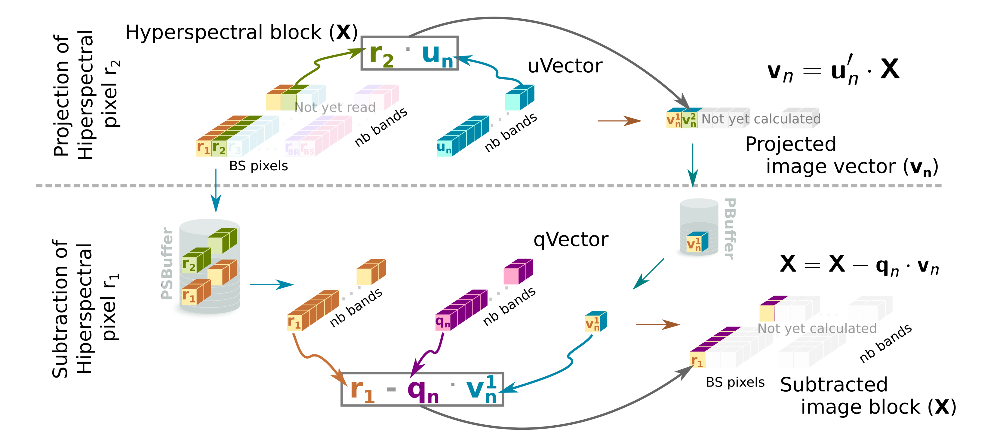
Proj_Sub 

Although this sub-module is represented by separate Projection and Subtraction boxes in Figure 2, it must be mentioned that both perform their computations in parallel. The Proj_Sub sub-module reads just once the hyperspectral block that was written in SBuffer by the Brightness sub-module ($\mathbf{X}$). Figure 6 shows an example of Projection and Subtraction stages. First, each hyperspectral pixel of the block is read by the Projection sub-module to obtain the projected image vector according to line 12 of Algorithm 1. At the same time, the hyperspectral pixel is written in PSBuffer, which can store two hyperspectral pixels. Two is the number of pixels because the Subtraction stage begins right after the first projection on the first hyperspectral pixel is ready, i.e., the executions of Projection and Subtraction are shifted by one pixel. Figure 6 shows such behavior. While pixel ${\mathbf{r}}_1$ is being consumed by Subtraction, pixel ${\mathbf{r}}_2$ is being written in PSBuffer. During the projection of the second hyperspectral pixel (${\mathbf{r}}_2$), the subtraction of the first one (${\mathbf{r}}_1$) can be performed since all the input operands, included the projection ${\mathbf{v}}_n$, are available, following the expression in line 13 of Algorithm 1.

The output of the Projection sub-module is the projected image vector, ${\mathbf{v}}_n$, which is forwarded to the HyperLCA Coder accelerator (through the Projection port) and to the Subtration sub-module (via the PBuffer FIFO). At the same time, the output of the Subtraction stage feeds the Loop_Iter block (see purple arrow, labeled as $\mathbf{X}$, in Figure 2) with the pixels of the transformed block in the $i^{th}$ iteration. It means that Brightness stage can start the next iteration without waiting to get the complete image subtracted. Thus, the initialization interval between loop-iterations is reduced as much as possible because the Brightness starts when the first subtracted data is ready.

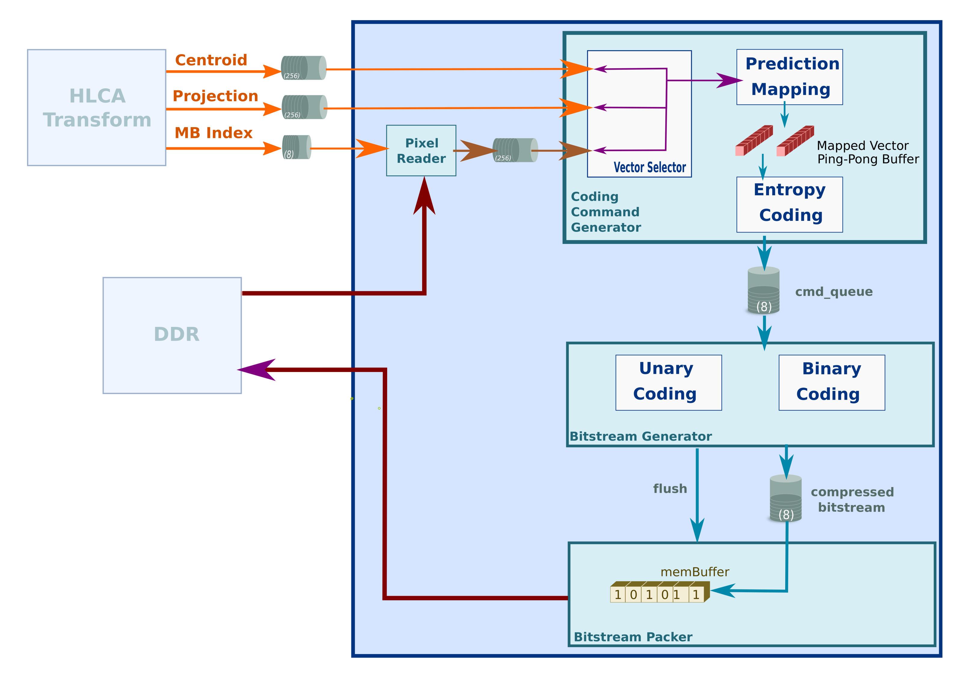
The FPGA-based solution described above highlights how the operations are performed in parallel to make the most out of such technology. Also, it has been spotted specific synchronization scenarios that are not possible to design using solely HLS. due to the current communication semantics supported by the synthesis tools. For example, is not possible for current synthesis tools to perform an analysis of the data and control dependencies such as the one done in this work. However, a hybrid solution based on HLS and hand-written VHDL code to glue the RTL models synthesized from C/C++ models, brings to life an efficient dataflow (see Figure 7). In this regard, the use of optimal sized FIFOs to interconnect the modules is key. For example, while the Brightness sub-module is filling the SBuffer, the Projection sub-module is draining it, and at the same time this sub-module supplies to the Subtraction sub-module with the same data read from SBuffer. Finally, Subtraction sub-module feeds back the Brightness sub-module through the BBuffer FIFO. The Brightness sub-module fills, in turn, the SBuffer, with the same data, closing the circle; this loop is repeated $p_{max}$ times.

Furthermore, the initialization interval between image blocks has been reduced. The task performed by the Avg sub-module for block $k+1$ (see Figure 7) can be scheduled at the same time that the Projection and Subtraction sub-modules are computing their outputs for block k, and right after the completion of the Brightness sub-module for block k. This is possible since the glue logic discards the output of the Subtraction sub-module during the last iteration. This logic ensures that the BBuffer is filled with the output from the Avg sub-module that feeds the first execution of Brightness for the first iteration of block $k+1$, resulting in an overlapped execution of the computation for blocks k and $k+1$.

Unfortunately, despite the optimizations introduced in the dataflow architecture, the HWacc is not able to reach the performance target as shown by the experimental results (see Section 3). The value in the column labeled as 1 PE (Processing Element) is clearly below the standard frame rates provided by contemporary commercial hyperspectral cameras. However, the number of FPGA resources required by the one-PE version of the HWacc is very low (see Section 3.2) which makes it possible to implement further parallelism strategies to speed up the compression process. Thus, three options open up for solving the performance problem.

First, task-level parallelism approach is possible by means of the use of several instances of the HWacc working concurrently. Second, increase the intra-HWacc parallelism using multiple operators, computing several pixel bands at the same time. Thirdly, a combination of the two previous approached. Independently of the strategy chosen, the limiting factor is the version of the Xilinx Zynq-7000 programmable SoC, that would have enough resources to support the design. In Section 4, a detailed analysis of several single-HWacc (with variations in the number of PEs) and multi-HWacc versions of the design is drawn.

So far, it has been described the inner architecture of a HWacc that only performs a computational operation over a single band component of a hyperspectral pixel. However, it can be modified to increase the number of bands that are processed in parallel. Thus, the HWacc of HyperLCA compressor turns from a single-PE to multiple PEs. This fact opens two new challenges. First challenge is to increase the width of the input and output ports of the modules, in accordance with the number of bands that would be processed in parallel. It must be mentioned that it is technologically possible because HLS-based solutions allow designers to build their own data types. For example, if a band component of a hyperspectral pixel is represented by an unsigned integer of 16-bits, we could define our own data type consisting of an unsigned integer of 160-bits packing ten bands of a hyperspectral pixel (see Figure 8). The second challenge has to do with the strategy to process the data in parallel. In this regard, a solution based on the map-reduce programming model has been followed.

Figure 8 shows an example of the improvements applied to the Cent stage, following the above-mentioned optimizations. The input of this stage is the hyperspectral block, ${\mathbf{M}}_k$, and the average pixel, $\widehat{\mathbf{\mu }}$, which are read in blocks of N-bands. The example assumes that the block is composed of ten bands and uses an user data type, specifically an unsigned int of 160-bits (10 bands by 16-bits to represent each band). Then, both blocks are broken down into the individual components that feed the PEs in an orderly fashion. This process is also known as map phase in the map-reduce programming model [45]. It must be mentioned that the design needs as many PEs as number of divisions made in the block.

Once the PEs have performed the assigned computational operation, the reduce phase of the map-reduce model is executed. For Cent sub-module, this stage consists of gathering in a block the partial results produced by each one of the PEs. Thus, a new block of N-bands is built, which in turn is part of the centralized block ($\mathbf{C}$), which is the output of Cent sub-module.

2.2.2. Coder

The HyperLCA Coder is the second of the HWacc developed, responsible for the error mapping and entropy-coding stages of the HyperLCA compression algorithm (Figure 1). The coder module teams up with the transform module to perform in parallel the CCSDS prediction error mapping [35] and the Golomb–Rice [36] entropy-coding algorithms as the different vectors are received from the HyperLCA Transform block.

The HyperLCA transform block generates the centroid, $\widehat{\mathbf{\mu }}$, extracted indexes of pixels, $j_{max}$, and projection vectors, ${\mathbf{v}}_n$, for an input hyperspectral block, ${\mathbf{M}}_k$. These arrays are consumed as they are received, reducing the need for large intermediate buffers. To minimize the necessary bandwidth to the memory that stores the hyperspectral image, only the indexes of the selected pixels in each iteration of the transform algorithm (line 8 of Algorithm 1) are provided to the coder (MB_index port).

The operation of the transform and coder blocks overlaps in time. Since the coder takes approximately half of the time the transform needs to generate each vector (see Section 3.2) for the maximum number of PEs (i.e., the maximum performance achieved), a contention situation is not taking place, reducing the pressure over the FIFOs that connect both blocks and, therefore, requiring less space for these communication channels.

Figure 9 sketches the internal structure of the HyperLCA Coder that has been modeled entirely using Vivado HLS. It is a dataflow architecture comprising three steps. During the first step, the prediction mapping and entropy coding of all the input vectors are performed by the coding command generator. The result of this step is a sequence of commands that are subsequently interpreted by the compressed bitstream generator.

The generation of the bitstream was extracted from the entropy-coding original functionality, which enabled a more efficient implementation of the latter, which could be re-written as a perfect loop and, therefore, Vivado HLS was able to generate a pipelined datapath with the minimum initiation internal (II = 1).

The generation of the compressed bitstream is simple. This module is continuously reading the cmd_queue FIFO for a new command to be processed. A command contains the operation (unary of binary coding) as well as the word (quotient or reminder, see Section 2.1.5) to be coded, and the number of bits to generate. Unary and binary coding functions simply iterate over the word to be coded and produces a sequence if bits which corresponds to the compressed form of the hyperspectral block.

Finally, the third step packs the compressed bitstream in words and written to memory. For this implementation, the width of the memory word is 64 bits, the maximum allowed by the AXI Master interface port for the Zynq-7020 SoC. The bitstream packer module instantiates a small buffer (64 words) that is flushed to DDR memory once it has been filled. This way, average memory access cycles per word is optimized by means of the use of burst requests.

As mentioned above, the HyperLCA Transform block feeds the coder with the indexes of the extracted pixels ${\mathbf{e}}_n$, which correspond to the highest brightness as the hyperspectral block is processed. Hence, it is necessary to retrieve the nb spectral bands from memory before the coder could start generating the compressed stream for the pixel vector. This is the role played by the pixel reader module. As in the case of the bitstream packer step, the pixel reader makes it use of a local buffer and issue burst requests to read the bands in the minimum number of cycles.

While the computing complexity of the coder module is low, the real challenge when it comes to the implementation of its architecture is to write a C++ HLS model that is consistent through the whole design, verification and implementation processes. To achieve this goal, it has been provided the communication channels with extra semantic so as to keep the different stages sync, despite the fact the model of computation of the architecture falls into the category of GALS (Globally Asynchronous, Locally Synchronous) systems. Side-channel information is embedded in the cmd_queue and compressed_stream FIFOs that connects the different stages of the coder. This information is used by the different modules to reset their internal states or stop and resume their operation (i.e., special commands to be interpreted by the bitstream generator or a flush signal as input to the packing module). This way, it is possible to integrate under a single HLS design all the functionality of the coder, which simplifies and speeds up the design process. On top of that, this strategy allowed avoiding the need to tailor the C++ HLS specification to make it usable in different steps of the design process. For example, it is common to write variations of the model depending on whether functional (C simulation) or RTL verification (co-simulation) is taking place due to the fact that the former is based on an untimed model and the latter introduces timing requirements [46,47].

Designing for parallelism is key to obtain the maximum performance. The dataflow architecture of the coder ensures an inter-module level of concurrency. However, the design must be balanced as to the latency of the different stages in the dataflow. Otherwise, the final result could be jeopardized. As mentioned before, decoupling the generation of the compressed bitstream from the entropy-coding logic, led to a more efficient implementation of the latter by the HLS synthesis tool. Also, this change helped to redistribute the computing effort, achieving a more balanced implementation.

In the first stage of the dataflow (coding command generator) a simple logic that controls the encoding of each input vector plus a header is implemented. It is an iterative process that performs the error mapping and error coding over the centroid, and $p\_max$ times over the extracted pixels and projections vectors. The bulk of this process is, thus, the encoding algorithm. The encoding is delegated in another module that implements an internal dataflow itself. In this way, it is possible to reduce the interval between two encoding operations. As can be seen in Figure 9, the prediction mapping and entropy-coding sub-modules communicates through a ping-pong buffer for the mapped vector.

To conclude this section, it is worth mentioning a couple of optimizations carried out related to the operations pow and log, which are used by the prediction mapping and entropy-coding algorithms. This type of arithmetic operation is costly to implement in FPGAs since the generated hardware is based on tables that consume on-chip resources (mainly BRAM memories), and an iterative processes that boosts latency. Since the base used in this application is 2, it can be largely simplified. Thus, we can substitute the pow and log operations by a logical shift instruction and the GCC compiler __builtin_clz(x) built-in function, respectively. This change is part of the refactoring process of the reference code implementation (golden model) that is almost mandatory at the beginning of any HLS project. The __builtin_clz(x) function is synthesizable and counts the leading zeros of the integer x. Therefore, the computation of the lowest power of 2 higher than M, performed during the entropy coding, is redefined as follows:

Listing 1. FGPA implementation of costly arithmetic operations during entropy encoding

1 //Original code 2 b = log2(M) + 1; 3 difference = pow(2,b) − M; 4  5 //FPGA optimization 6 b = (32 − __builtin_clz(M)); 7 difference = (1<<b) − M;

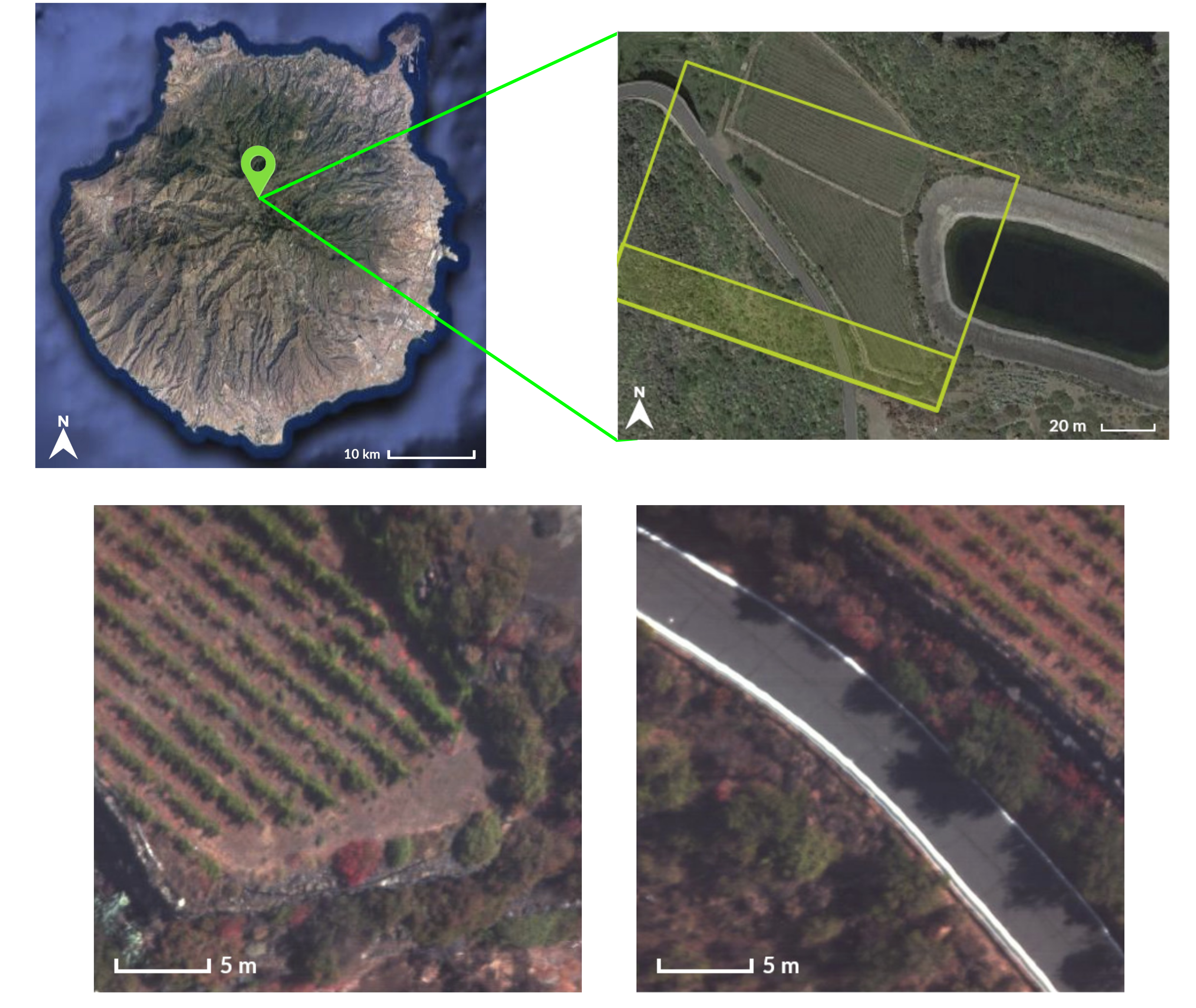
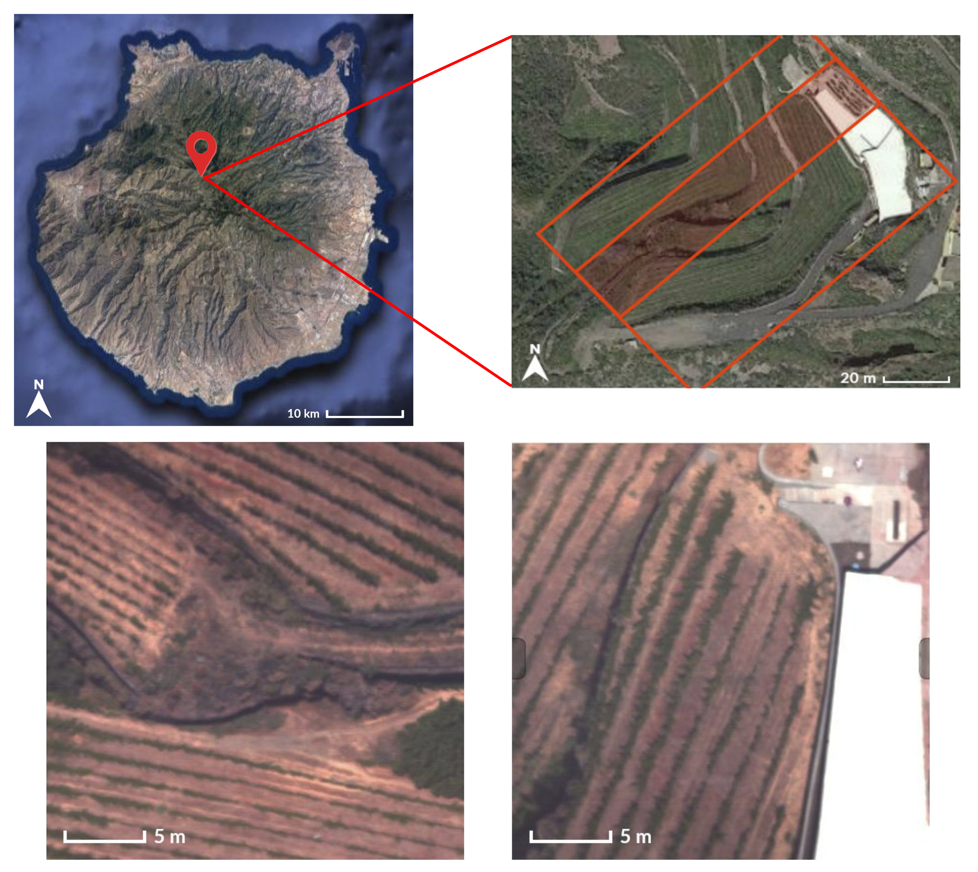
2.3. Reference Hyperspectral Data

In this section, we introduce the hyperspectral imagery used in this work to evaluate the performance of the proposed computing approach using reconfigurable logic devices. This data set is composed of 4 hyperspectral images that were also employed in [29], where the HyperLCA algorithm was implemented in low-power consumption embedded GPUs. We have kept the same data set in order to compare in Section 3 the performance of the developed FPGA-based solution with the results obtained by the GPU accelerators.

In particular, the test bench was sensed by the acquisition system extensively analyzed in [48]. This aerial platform mounts a Specim FX10 pushbroom hyperspectral camera on a DJI Matrice 600 drone. The image sensor covers the range of the electromagnetic spectrum between 400 and 1000 nm using 1024 spatial pixels per scanned cross-track line and 224 spectral bands. Nevertheless, the hyperspectral images used in the experiments only retain the spectral information of 180 spectral bands. Concretely, the first 10 spectral bands and the last 34 bands have been discarded due to the low spectral response of the hyperspectral sensor at these wavelengths.

The data sets were collected over some vineyard areas in the center of Gran Canaria island (Canary Islands, Spain) and in particular, in a village called Tejeda, during two different flight campaigns. Figure 10 and Figure 11 display some Google Maps pictures of the scanned terrain in both flight missions, whose exact coordinates are 27°59′35.6″N 15°36′25.6″W (green point in Figure 10) and 27°59′15.2″N 15°35′51.9″W (red point in Figure 11), respectively. Both flight campaigns were performed at a height of 45 m over the ground, which results in a ground sampling distance in line and across line of approximately 3 cm.

The former was carried out with a drone speed of 4.5 m/s and the camera frame rate set to 150 frames per second (FPS). In particular, this flight mission consisted of 12 waypoints that led to a total of 6 swathes, but only one was used for the experiments, which has been highlighted in green in Figure 10. Two portions of 1024 hyperspectral frames with all their 1024 hyperspectral pixels were selected from this swath to generate two of the data sets that compose the test bench. A closer view of these selected areas can be also seen in Figure 10. These images are false RGB representations extracted from the acquired hyperspectral data.

The latter was carried out with a drone speed of 6 m/s and the camera frame rate set to 200 FPS. The entire flight mission consisted of 5 swathes, but only one was used for the experiments in this work, which has been highlighted in red in Figure 11. From this swath, two smaller portions of 1024 hyperspectral frames were cut out for simulations. A closer view of these selected areas is also displayed in Figure 11. Once again, they are false RGB representations extracted from the acquired hyperspectral data. For more details about the flight campaigns, we encourage the reader to see [48].

3. Results

3.1. Evaluation of the HyperLCA Compression Performance

The goodness of the I12 version of the HyperLCA algorithm proposed in this work has been evaluated and compared with previous I32 and I16 versions of the algorithm presented in [37] and the single precision floating-point (F32) implementation presented in [29]. For doing so, the hyperspectral imagery described in Section 2.3 has been compressed/decompressed using different settings of the HyperLCA compressor input parameters.

In this context, the information lost after the lossy compression process has been analyzed using three different quality metrics. Concretely, the Signal-to-Noise Ratio (SNR), the Root Mean Squared Error (RMSE) and the Maximum Absolute Difference (MAD), which are shown in Equations (3)–(5), respectively. The SNR and the RMSE give an idea of the average information lost in the compression-decompression process. Bigger values of SNR are indicative of better compression performance. On the contrary, higher RMSE values mean that the lossy compression has introduced bigger data losses. The MAD assesses the amount of lost information for the worst reconstructed image value. For our targeted application, the dynamic range is $2^{12}=4096$ and hence, the worst possible MAD value is 4095. For the sake of clarity, the aforementioned metrics have been calculated using the entire compressed–decompressed images, i.e., after the HyperLCA algorithm has finished to compress all image blocks, ${\mathbf{M}}_K$.

$$\mathrm{SNR}=10·{log}_{10}\left(\frac{{\sum }_{i=1}^{nb}{\sum }_{j=1}^{np}{\left(I_{i,j}\right)}^2}{{\sum }_{i=1}^{nb}{\sum }_{j=1}^{np}{(I_{i,j}-I{c}_{i,j})}^2}\right)$$

(3)

$$\mathrm{RMSE}=\frac{1}{np·nb}·\sqrt{\sum _{i=1}^{nb}\sum _{j=1}^{np}{(I_{i,j}-I{c}_{i,j})}^2}$$

(4)

$$\mathrm{MAD}=\max (I_{i,j}-I{c}_{i,j})$$

(5)

Table 2. Comparison of the compression results for the four versions of the HyperLCA algorithm under study: I12, I16, I32 and F32.

Nbits	BS	CR	SNR				MAD				RMSE
			I12	I16	I32	F32	I12	I16	I32	F32	I12	I16	I32	F32
12		12	43.01	38.01	43.12	42.75	24.50	39.00	25.00	25.50	3.12	5.55	3.08	3.22
	1024	16	42.27	38.57	42.27	41.97	32.25	41.50	32.25	32.50	3.40	5.21	3.40	3.52
		20	41.31	39.13	41.31	41.06	41.25	46.50	41.25	41.25	3.73	4.88	3.80	3.91
		12	42.99	38.95	43.03	42.68	26.25	34.50	25.00	25.00	3.13	4.98	3.12	3.24
	512	16	42.45	39.36	42.47	42.14	30.75	38.00	30.00	30.50	3.33	4.75	3.33	3.45
		20	41.50	39.92	41.48	41.24	39.50	43.75	39.50	40.00	3.72	4.46	3.72	3.83
		12	43.03	40.00	43.02	42.67	25.00	34.50	25.00	25.50	3.12	4.42	3.12	3.25
	256	16	42.33	40.51	42.32	42.02	34.75	37.25	34.75	35.00	3.38	4.16	3.38	3.50
		20	40.94	40.59	40.59	40.73	54.75	57.75	54.75	54.75	3.96	4.13	3.97	4.06
8		12	41.80	36.91	42.19	41.68	23.25	41.50	22.00	22.25	3.62	6.32	3.47	3.69
	1024	16	41.63	37.42	41.73	41.27	25.50	41.25	25.50	26.50	3.69	5.95	3.65	3.86
		20	41.20	37.89	41.20	40.79	32.25	42.00	32.50	32.25	3.87	5.64	3.87	4.07
		12	42.49	37.99	42.70	42.26	23.00	38.00	22.75	22.25	3.33	5.57	3.25	3.42
	512	16	42.07	38.64	42.09	41.69	27.50	36.00	26.50	26.75	3.49	5.17	3.48	3.65
		20	41.61	39.01	41.60	41.25	31.25	39.50	30.50	31.75	3.68	4.95	3.68	3.84
		12	42.79	39.35	42.82	42.39	24.75	35.50	25.00	25.00	3.20	4.76	3.19	3.36
	256	16	42.15	39.96	42.13	41.76	30.00	37.00	29.75	29.75	3.45	4.43	3.46	3.61
		20	41.80	40.21	41.78	41.44	35.75	37.00	35.75	36.00	3.59	4.31	3.60	3.74

shows the average results obtained for each configuration of the HyperLCA compressor input parameters using the data set described in Section 2.3. Different conclusions can be drawn from these results. First of all, it is confirmed that the I12 version offers significantly better-quality compression results than previous I16 version, employing the same hardware resources. These gaps are even wider for smaller compression ratios. This is because the losses introduced by the decrease in the data precision compare to the previous I16 version, as mentioned in Section 2.1.6, is disguised by the bigger losses introduced by the compression process itself for higher compression ratios.

Additionally, deviations in the values of the three quality metrics employed in this work between I32, I12 and F32 versions are almost negligible, with the advantage of halving the memory space required for storing $\mathbf{C}$. Second, it can be also concluded that the HyperLCA lossy compressor is able to compress the hyperspectral data with high compression ratios and without introducing significant spectral information losses.

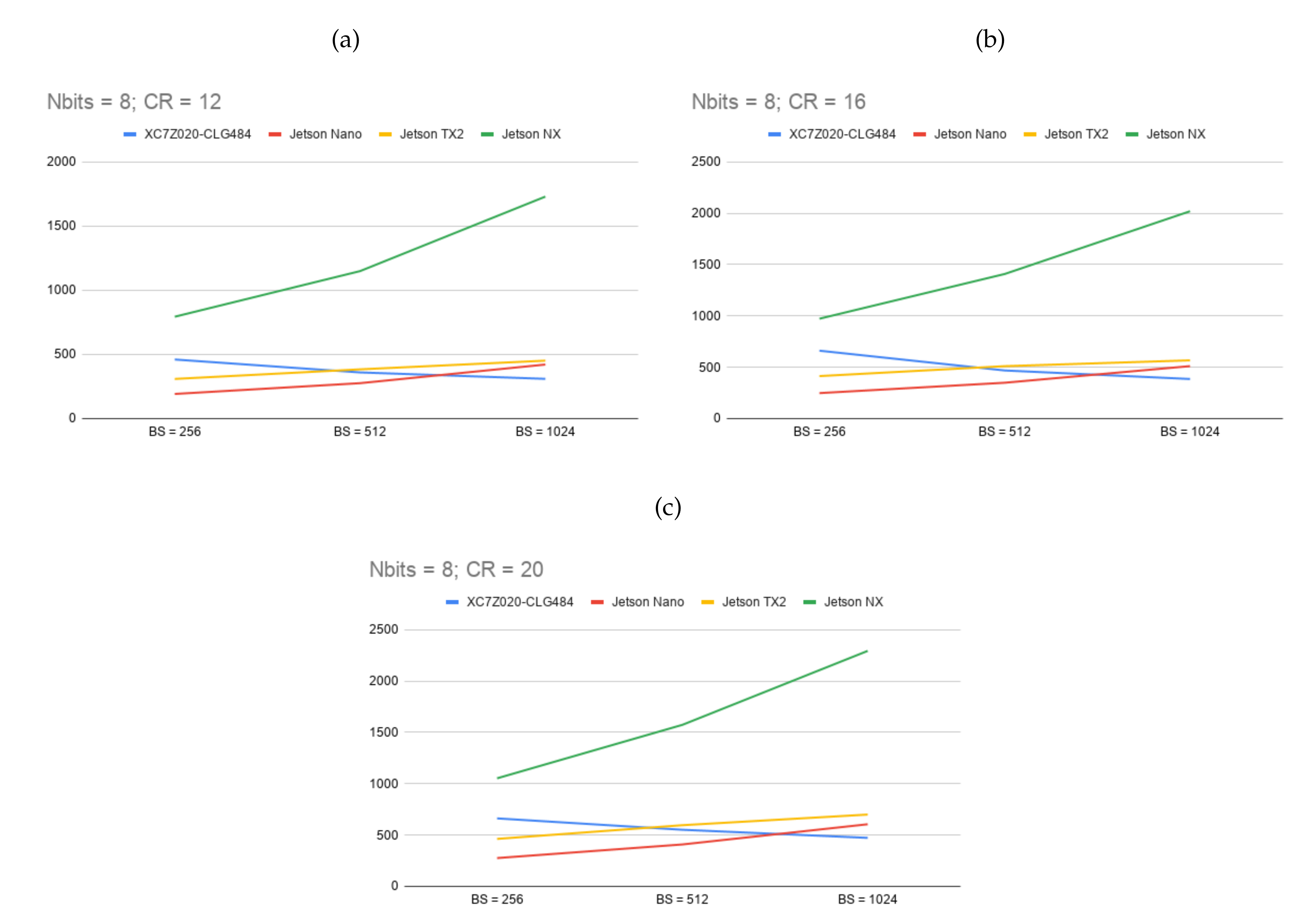
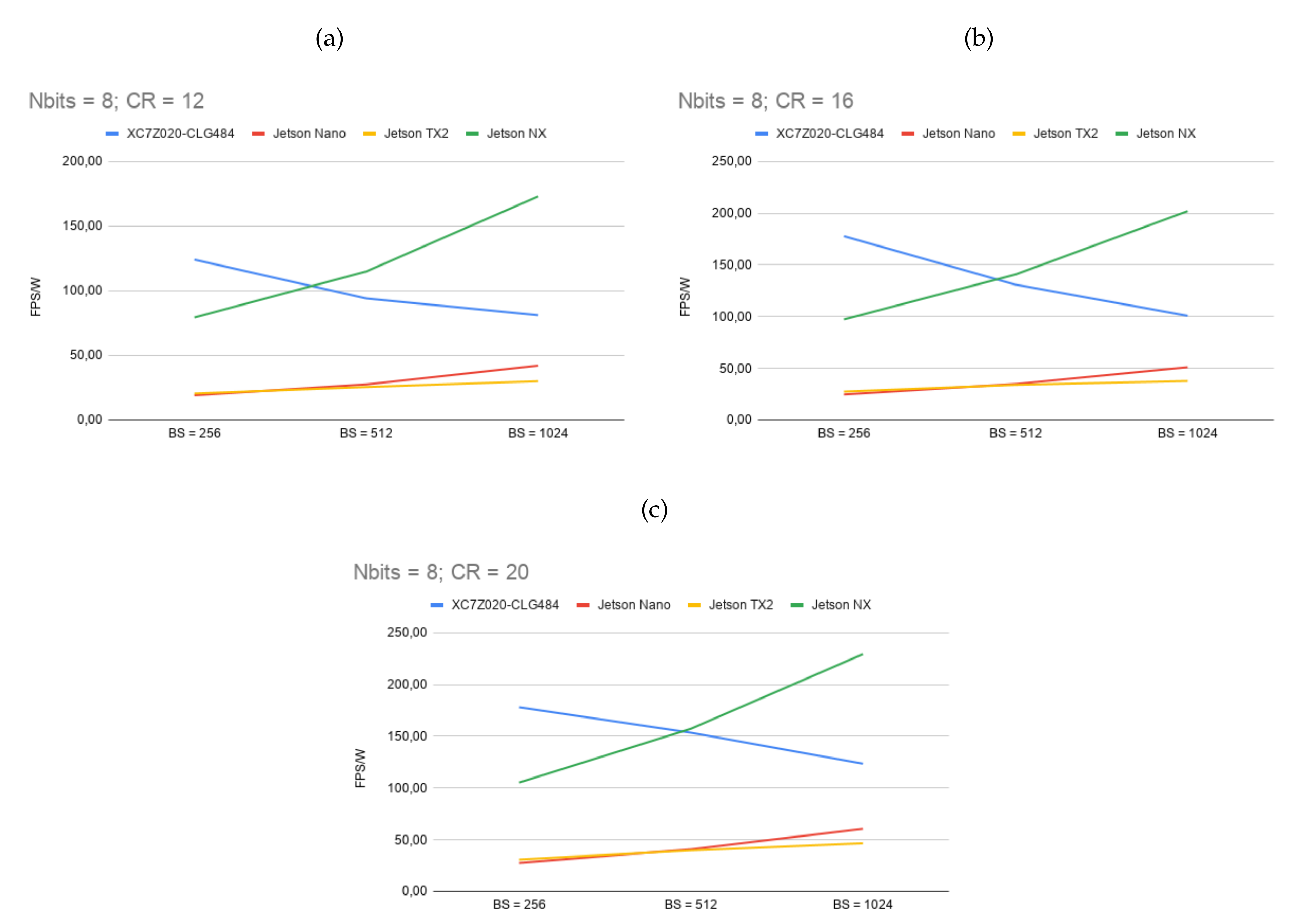
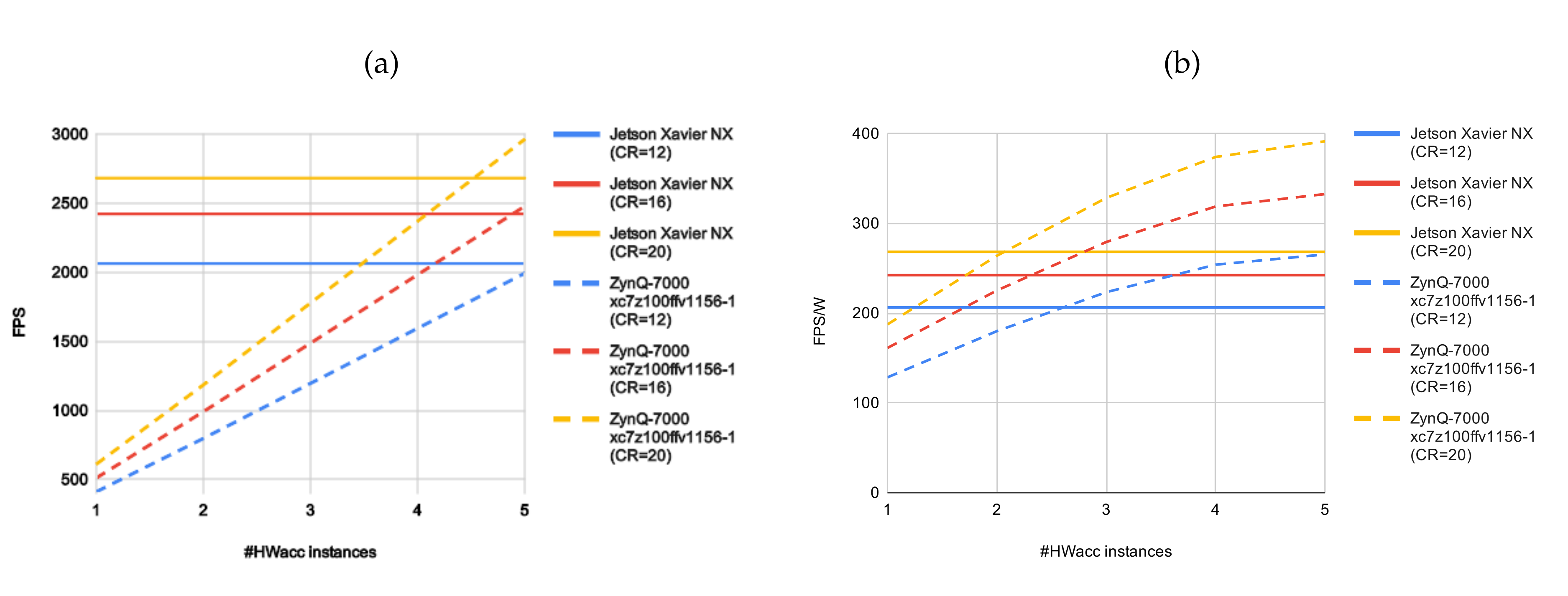
3.2. Evaluation of the HyperLCA Hardware Accelerator

Section 2.1 describes the FPGA-based implementation of the HyperLCA compressor as defined in Algorithm 1. The architecture of the HWacc is divided into two blocks, Transform and Coder that run in parallel following a producer-consumer approach. Therefore, for the performance analysis of the whole solution, the slowest block is the one determining the productivity of the proposed architecture.

The HyperLCA Transform block bears most of the complexity and computational burden of the compression process. For that reason, several optimizations (see Section 2.1.3) have been applied during its design in order to achieve a high degree of parallelism and, thus, reduce the latency. One of the most important improvements is the realization of the map-reduce programming model, to enable an architecture with multiple PEs (see Figure 8) working concurrently on several bands. The experiments carried out over the different alternatives for the HyperLCA Transform block are intended to evaluate how the performance and resource usage of the FPGA-based solution scales, as the number of PEs instantiated by the architecture grows up.

The configuration of the input parameters has been set as follows: CR parameter has been set to 12, 16 and 20; the BS parameter has been set to 1024, 512 and 256 and; $N_{bits}$ parameter gets the values 12 and 8. The value of $p_{max}$ is obtained at design time from these parameters following Equation (1), and are listed in the last column of

Table 3. Design-time configurations parameters of the HyperLCA transform hardware block for hyperspectral images with 180 bands.

${\mathit{N}}_{\mathbf{bits}}$	BS	CR	Min SBuffer Depth						${\mathit{p}}_{\mathbf{max}}$
			1 PE	2 PEs	4 PEs	6 PEs	10 PEs	12 PEs
12		12							12
	1024	16	184,320	92,160	46,080	30,720	18,432	15,360	9
		20							7
		12							10
	512	16	92,160	46,080	30,720	18,432	15,360	7680	8
		20							6
		12							8
	256	16	46,080	30,720	18,432	5,360	7680	3840	6
		20							4
8		12							17
	1024	16	184,320	92,160	46,080	30,720	18,432	15,360	13
		20							10
		12							14
	512	16	92,160	46,080	30,720	18,432	15,360	7680	10
		20							8
		12							10
	256	16	46,080	30,720	18,432	15,360	7680	3840	7
		20							6
Data Width (bits)			16	32	64	96	160	192

. Concerning the sizing of the various memory elements present in the architecture, it is determined by two parameters: the number of PEs to instantiate (parallel processing of hyperspectral bands) and the size of the image block to be compressed. It is worth mentioning that in this version of the HWacc, the number of PEs must be a divisor of the number of hyperspectral bands in order to simplify the design of the datapath logic.

First, the data width of the architecture must be defined. Such parameter is obtained multiplying the number of PEs by the size of the data type used to represent a pixel band. In the version of the HWacc under evaluation, the I12 alternative has been selected, due to its good behavior (comparable to the I32 version as discussed in Section 2.1.6) and the resource savings it brings. For the I12 version, a band is represented with an unsigned short int which turns into 16-bit words in memory. On the contrary, choosing the I32 version, the demand for memory resources and internal buffers (such as the SBuffer) would double, because an unsigned int data type is used in the model definition. Thus, if the HWacc only instantiates a PE, the data width will be 16-bits, whereas if the HWacc instantiates 12 PEs (i.e., the HWacc performs 12 operations over the set of bands in parallel), the data width will be 192-bits. Second, the depth of the SBuffer must be calculated following Equation (6), where BS is the block size, nb the number of bands (in our case is fixed to 180), and $N_{PEs}$ is the number of processing elements.

$$SBufferDept{h}_{min}=\frac{BS·nb}{N_{PEs}}$$

(6)

Being optimal as to the use of BRAM blocks within the FPGA fabric is compulsory since this resource is highly demanded as the number of PEs increases (seen in

Table 4. Post-Synthesis results for the different versions of the HyperLCA Transform for a Xilinx Zynq-7020 programmable SoC and image block up to 180 bands.

BS	Num. PEs	BRAM18K		DSP48E		FlipFlops		LUTs
256	1	56	(20.0%)	9	(4.09%)	6942	(6.52%)	5194	(9.76%)
	2	59	(21.07%)	16	(7.27%)	9112	(8.56%)	8735	(16.42%)
	4	71	(25.36%)	30	(13.64%)	20,171	(18.96%)	15,811	(29.72%)
	6	71	(25.36%)	62	(28.18%)	29,368	(27.6%)	23,530	(44.23%)
	10	84	(30.0%)	102	(46.36%)	47,350	(44.5%)	38,221	(71.84%)
	12	71	(25.36%)	122	(55.45%)	56,297	(52.91%)	45,867	(86.22%)
512	1	101	(36.07%)	9	(4.09%)	6988	(6.57%)	5270	(9.91%)
	2	102	(36.43%)	16	(7.27%)	9159	(8.61%)	8820	(16.58%)
	4	113	(40.36%)	30	(13.64%)	20,215	(19.0%)	16,040	(30.15%)
	6	113	(40.36%)	62	(28.18%)	29,406	(27.64%)	23,761	(44.66%)
	10	124	(44.29%)	102	(46.36%)	47,420	(44.57%)	38,352	(72.09%)
	12	113	(40.36%)	122	(55.45%)	56,342	(52.95%)	45,857	(86.20%)
1024	1	192	(68.57%)	9	(4.09%)	7114	(6.69%)	5468	(10.28%)
	2	190	(67.86%)	16	(7.27%)	9278	(8.72%)	8969	(16.86%)
	4	198	(70.71%)	30	(13.64%)	20,301	(19.08%)	16,210	(30.47%)
	6	199	(71.07%)	62	(28.18%)	29,524	(27.75%)	23,916	(44.95%)
	10	204	(72.86%)	102	(46.36%)	47,514	(44.66%)	38,485	(72.34%)
	12	199	(71.07%)	122	(55.45%)	56,463	(53.07%)	46,116	(86.68%)

). On top of that, keeping the use of resources under control brings along some benefits such as helping the synthesis tool to generate a better datapath and, therefore, to obtain an implementation with a shorter critical path or contain the consumption of energy.

Table 3 lists the memory requirements demanded by SBuffer for the 108 different configurations of the HyperLCA Transform block evaluated in this work. The SBuffer component is, by far, the largest memory instantiated by the architecture and it is implemented as a FIFO. SBuffer component has been generated with the FIFO generator tool provided by Xilinx which only allows depths that are power of two. Therefore, from a technical point of view, it is not possible to match the minimum required space of SBuffer with the obtained from the vendor tools. To mitigate the waste of memory space derived from such constraint of the tool, the SBuffer has been broken into two concatenated FIFOs (i.e., the output of the first FIFO is the input of the second) but keeping the facade of a single FIFO to the rest of the system. For example, the minimum depth of SBuffer for $PE=1$ and $BS=256$ is 46,080. With a single FIFO, the smallest depth with enough capacity generated by Xilinx tools would be 65,536. Therefore, the unused memory space represents approximately 30% of the overall resources for SBuffer. However, by using the double FIFO approach, one FIFO of 32,768 words plus another one of 16384 would be use. Only ≈ 6% of the assigned resources to SBuffer would be misused.

To evaluate the HyperLCA Transform hardware accelerator, the proposed HWacc architecture has been implemented using the Vivado Design suite. This toolchain is provided by Xilinx and features a HLS tool (Vivado HLS) devoted to optimize the developing process of IP (Intellectual Property) components FPGA-based solutions for their own devices. The first implemented prototype instantiated one HWacc targeting the XC7Z020-CLG484 version of the Xilinx Zynq-7000 SoC. This FPGA has been selected because of its low-cost, low-weight and high flexibility, features that make it an interesting device to be integrated in aerial platforms, such as drones. The aim of this first prototype is to evaluate the capability of a mid-range reconfigurable FPGAs such as the XC7Z020 chip, for a specific application such as the HyperLCA compression algorithm. Hence, and due to the amount of resources available on the target device, the maximum possible number of PEs for the single-HWacc prototype is 12.

Table 4 summarizes the resources required, which have been extracted from post-synthesis reports, for each of the 108 versions of the HWacc that process different block sizes of 180-band hyperspectral images of the data set (see Section 2.3).

Several conclusions can be derived from these figures. In first place, the amount of digital signal processors (DSPs), flipflops (FFs) and look-up-tables (LUTs) resources increases with the number of PEs but are similar for different values of the BS parameter. On the contrary, the demand of BRAMs depends directly on BS and increases slightly with PE for a given block size. The $PE=10$ version needs a special remark. Such version represents an anomaly in the linear behavior of the resource demand. Even with the use of a double FIFO approach, as explained before, the total capacity of the BRAM used to instantiate SBuffer is clearly oversized for that datawidth to assure that a hyperspectral block and its transformations (${\mathbf{M}}_k$ and $\mathbf{C}$, respectively) could be stored in-circuit. Second, in addition to the resources needed by the HWacc of the HyperLCA Transform, it is necessary to take into account those corresponding to the other components in the system such as the Coder or the DMA (Direct Memory Access) to move the hyperspectral data (${\mathbf{M}}_k$) from/to DDR to/from the hardware accelerators. These extra components will make use of the remaining resources (specially LUTs, which is the most demanded as can be seen in Table 4), establishing a maximum of 12 for the number of PEs.

Table 5. Post-Synthesis results for the HyperLCA Coder block for a Xilinx Zynq-7020 programmable SoC and pixel size up to 180 bands.

BS	BRAM18K		DSP48E		FlipFlops		LUTs
2,565,121,024	7	(2.5%)	1	(0.45%)	3464	(3.25%)	4106	(7.71%)

shows the post-synthesis results for the HyperLCA Coder block. The resources demanded by the coder does not depend on the BS parameter or the number of PEs. It is important to mention that the majority of the BRAM, FFs and LUTs resources are assigned to the two AXI-Memory interfaces that the HLS tool generates for the Pixel Reader and the Bitstream Packer modules (see Figure 9).

Table 6. Maximum frame rate obtained using the FPGA-based solution on a Xilinx ZynQ-7020 programmable SoC for hyperspectral images with 180 bands.

			Max Frame Rate
${\mathit{N}}_{\mathbf{bits}}$	BS	CR	1 PE		2 PEs		4 PEs		6 PEs		10 PEs		12 PEs
			$f_1$	$f_2$	$f_1$	$f_2$	$f_1$	$f_2$	$f_1$	$f_2$	$f_1$	$f_2$	$f_1$	$f_2$
12		12	37	56	72	108	131	196	178	266	248	370	275	411
	1024	16	47	71	91	137	167	250	225	336	310	463	343	511
		20	58	87	112	168	204	305	273	408	373	555	410	611
		12	43	65	83	125	152	228	205	307	284	424	314	469
	512	16	52	78	100	151	183	273	245	366	336	501	370	552
		20	69	98	126	189	229	342	304	454	411	612	452	672
		12	52	78	100	149	181	270	242	361	330	493	364	543
	256	16	65	97	125	187	227	339	301	449	405	604	444	661
		20	87	130	167	251	303	453	397	591	523	778	570	847
8		12	27	41	53	79	96	144	131	197	186	278	207	310
	1024	16	34	52	67	100	122	183	166	248	232	347	258	386
		20	43	65	84	126	153	229	206	309	286	427	317	473
		12	32	49	62	94	114	170	155	232	217	324	241	360
	512	16	43	65	83	125	152	227	205	307	284	424	370	469
		20	52	78	100	151	183	273	245	366	336	501	370	552
		12	43	65	83	124	150	225	202	303	279	417	309	460
	256	16	57	86	111	166	201	301	268	401	364	543	400	596
		20	65	97	125	187	227	339	301	448	405	603	444	661

$f_1$ Clock frequency: 100 MHz. $f_2$ Clock frequency: 150 MHz.

shows the throughput, expressed as the maximum frame rate, for a specific configuration of the HWacc using two clock frequencies: 100 MHz and 150 MHz (

Table A1. Evaluation of the results obtained using the FPGA-based solution on a Xilinx Zynq-7020 programmable SoC for hyperspectral images with 180 bands.

${\mathit{N}}_{\mathbf{bits}}$	BS	CR	Cycles per Block												${\mathit{p}}_{\mathbf{max}}$
			(Max Frame Rate)
			1 PE		2 PEs		4 PEs		6 PEs		10 PEs		12 PEs
			100 MHz	150 MHz	100 MHz	150 MHz	100 MHz	150 MHz	100 MHz	150 MHz	100 MHz	150 MHz	100 MHz	150 MHz
12		12	2,666,775		1,388,085		763,648		563,553		404,613		364,594		12
			37	56	72	108	131	196	178	266	248	370	275	411
	1024	16	2,093,523		1,088,779		599,742		445,886		323,820		293,101		9
			47	71	91	137	167	250	225	336	310	463	343	511
		20	1,711,355		889,312		490,447		367,439		269,887		245,360		7
			58	87	112	168	204	305	273	408	373	555	410	611
		12	1,145,407		596,547		328,928		244,157		176,829		159,901		10
			43	65	83	125	152	228	205	307	284	424	314	469
	512	16	953,703		496,418		273,941		204,570		149,589		135,691		8
			52	78	100	151	183	273	245	366	336	501	370	552
		20	761,999		396,125		218,877		165,082		122,367		111,546		6
			69	98	126	189	229	342	304	454	411	612	452	672
		12	479,335		250,030		138,409		103,597		76,005		69,030		8
			52	78	100	149	181	270	242	361	330	493	364	543
	256	16	382,863		199,499		110,479		83,400		62,056		56,649		6
			65	97	125	187	227	339	301	449	405	604	444	661
		20	286,391		148,931		82,691		63,382		48,200		44,265		4
			87	130	167	251	303	453	397	591	523	778	570	847
8		12	3,622,195		1,886,981		1,036,739		759,669		539,143		483,832		17
			27	41	53	79	96	144	131	197	186	278	207	310
	1024	16	2,857,859		1,487,981		818,201		602,802		431,461		388,391		13
			34	52	67	100	122	183	166	248	232	347	258	386
		20	2,284,607		1,188,572		654,337		485,088		350,730		316,731		10
			43	65	84	126	153	229	206	309	286	427	317	473
		12	1,528,815		797,038		438,876		323,247		231,359		208,129		14
			32	49	62	94	114	170	155	232	217	324	241	360
	512	16	1,145,407		596,571		328,949		244,100		176,809		159,834		10
			43	65	83	125	152	227	205	307	284	424	370	469
		20	953,703		496,495		274,002		204,592		149,566		135,748		8
			52	78	100	151	183	273	245	366	336	501	370	552
		12	575,808		300,575		166,183		123,677		89,908		81,374		10
			43	65	83	124	150	225	202	303	279	417	309	460
	256	16	431,099		224,781		124,409		93,463		68,997		62,850		7
			57	86	111	166	201	301	268	401	364	543	400	596
		20	382,863		199,486		110,540		83,520		62,093		56,658		6
			65	97	125	187	227	339	301	448	405	603	444	661

extends this information by adding the number of cycles to compute a hyperspectral block). Columns labeled as PE denote the number of processing elements instantiated by the HWacc, which in combination with the input parameters ($N_{bits}$, BS, CR and $p_{max}$), show the average number of hyperspectral blocks that the HWacc is able to compress per second (FPS). The maximum frame rate has been normalized to 1024 hyperspectral pixels per block, which is the size of the frame delivered by the acquisition system.

It is worth noting that these results include the transform and coding steps, which are performed in parallel.

Table 7. Comparison of the computation effort made by the Transform and Coding stages.

${\mathit{N}}_{\mathbf{bits}}$	BS	CR	Cycles per Block		${\mathit{p}}_{\mathbf{max}}$
			Transform Delay (12 PEs)	Coder Delay
12		12	364,594	184,999	12
	1024	16	293,101	137,379	9
		20	245,360	105,836	7
		12	159,901	88,235	10
	512	16	135,691	70,468	8
		20	111,546	52,593	6
		12	69,030	44,095	8
	256	16	56,649	33,294	6
		20	44,265	22,587	4
8		12	483,832	194,170	17
	1024	16	388,391	147,055	13
		20	316,731	111,919	10
		12	208,129	94,584	14
	512	16	159,834	67,697	10
		20	135,748	54,037	8
		12	81,374	44,579	10
	256	16	62,850	31,424	7
		20	56,658	27,163	6

shows the coding times (in clock cycles) compared to the time needed by the transform step with the best configuration possible (i.e., $PE=12$). The HyperLCA Coder takes roughly 50% less time on average and, since the relation between both hardware components is a dataflow architecture, the latency of the whole process corresponds to the maximum; that is, the delay of the Transform step.

One key factor is the minimum frame rate that must be supported for the targeted application. Ideally, such threshold would correspond to the maximum frame rate provided by the employed hyperspectral sensor (i.e., 330 FPS). However, the experimental validation of the camera set-up in the drone (Section 2.3), tells us that frame rates between 150 and 200 are enough to obtain hyperspectral images with the desired quality, given the speed and altitude of the flights. Therefore, a threshold value of 200 FPS is established as the minimum throughput to validate the viability of the HyperLCA hardware core. In Table 7, it has been highlighted (bold type-faced cells) the configurations that would be valid given this minimum. Thus, it can be observed that the $PE=12$ version, for both clock frequencies, and the $PE=10$ version at 150 MHz reach the minimum frame rate, even for the most demanding scenario ($N_{bits}=8$, $BS=1024$ and $CR=12$). In turn, by using lower values for $N_{bits}$ the compression rate is reduced due to the higher number of $\mathbf{V}$ vectors extracted by the HyperLCA Transform. This means that more computations must be performed to compress a hyperspectral block. It must be mentioned that the $PE=10$ version meets the FPS target in all the scenarios but the most demanding one when the clock frequency is set to 100 MHz. As for the $PE=10$ version, the $PE=6$ version does not reach the minimum FPS in a few scenarios (concentrated in $N_{bits}=8$ and $BS=1024$), but in can be a viable solution given the actual needs of the application set-up.

In addition to the performance results listed in Table 6, Figure 12 graphically shows the speed-up gained by the FPGA-based implementation as the number of PEs increases. The values have been normalized, using the average time for the $PE=1$ version as the baseline. Several conclusions can be drawn from this figure. First, it is observable that the $PE=12$ version of the HWacc performs ×7 times ($N_{bits}=12$) to ×7.6 times ($N_{bits}=8$) faster than $PE=1$ version. This configuration is the one that guarantees the fastest compression results. Second, the speed-up gain is nearly linear for $PE=2$ and $PE=4$ versions, whereas the scalability of the accelerator drops as the number of PEs is higher (see Figure 12a,b). This behavior is seen for both $N_{bits}=8$ and $N_{bits}=12$ configurations (see Figure 12c,d). However, for higher values of $BS$ and $CR$ the shape of the curve shows a better trend though not reaching the desired linear speed-up.

4. Discussion

In this paper, we present a detailed description of an FPGA-based implementation of the HyperLCA algorithm, a new lossy transform-based compressor. As fully discussed in Section 3.2, the proposed HWacc meets the requirements imposed by the targeted application in terms of the frame rate range employed to capture quality hyperspectral images. In this section, we would like to also provide a comprehensive analysis of the suitability of the FPGA-based HyperLCA compressor implementation and a comparison with the results obtained by an embedded System-on-Module (SoM) based on a GPU that has been recently published [29].

Concretely, María Díaz et al. introduce in [29] three implementation models of the HyperLCA compressor. In this previous work, the parallelism inherent to the HyperLCA algorithm was exploited beyond the thread-level concurrency of the GPU programming model taking advantage of the CUDA steams. In particular, the third approach, referred to as Parallel Model 3 in [29], achieves the highest speed-up, especially for bigger image blocks ($BS=1024$). This implementation model bets for pipelining the data transfers between the host and the device and the kernel executions for the different image blocks (${\mathbf{M}}_k$). To do this, such proposal exploits the benefits of the concurrent kernel execution through the management of CUDA streams. Unlike the FPGA-based implementation model proposed in this paper, only the HyperLCA Transform stage is accelerated in the GPU. In this case, the codification stage is also pipelined with the HyperLCA Transform stage but executed on the Host using another parallel CPU process. Table 2 collects the quality results of the compression process issued by the aforementioned GPU-based implementation model in terms of SNR, MAD and RMSE (F32 version). For more details, we encourage the reader to see [29].

To compare the performance of the GPU-based implementation model and the FPGA solution presented here, we are going to use two assessment metrics: the maximum number of frames compressed in a second (FPS) and the power efficiency in terms of FPS per watt. The latter figure of merit is of great importance given the target application, since it is critical to maximize the battery life of the drone. Additionally, the GPU-based model introduced in [29] has been executed in three different NVIDIA Jetson embedded computing devices: Jetson Nano, Jetson TX2 and the most recent supercomputer Jetson Xavier NX.

These modules have been selected for the reasonable computational power provided at a relatively low power consumption.

Table 8. Most relevant characteristics of the NVIDIA modules Jetson Nano, Jetson TX2 and Jetson Xavier NX.

	Jetson Nano
LPGPU	GPU NVIDIA Maxwell architecture with 128 NVIDIA CUDA cores
CPU	Quad-core ARM Cortex-A57 MPCore processor
Memory	4 GB LPDDR4, 1600MHz 25.6 GB/s
	Jetson TX2
LPGPU	GPU NVIDIA Pascal with 256 CUDA cores
CPU	HMP Dual Denver 2/2 MB L2 + Quad ARM A57/2 MB L2
Memory	8 GB LPDDR4, 128 bits bandwidth, 59.7 GB/s
	Jetson Xavier NX
LPGPU	GPU NVIDIA Volta with 384 NVIDIA CUDA cores and 48 Tensor cores
CPU	6-core NVIDIA Carmel ARM®v8.2 64-bit CPU 6 MB L2 + 4 MB L3
Memory	8 GB 128-bit LPDDR4x @ 51.2GB/s

summarizes the most relevant technical characteristics of these embedded computing boards. As can be seen, the Jetson Nano module integrates the less advanced, oldest generation of the three GPU architectures, instantiating the fewer execution units or CUDA cores as well. On the contrary, Jetson Xavier NX represents one of the latest NVIDIA power-efficient products, which offers more than 10X the performance of its widely adopted predecessor, Jetson TX2.

Table 9. Maximum frame rates obtained by the proposed FPGA implementation and the GPU-based model introduced in [29] for the NVIDIA boards Jetson Nano, Jetson TX2 and Jetson Xavier NX.

			Max Frame Rate
			FPGA		GPU
${\mathit{N}}_{\mathbf{bits}}$	BS	CR	XC7Z020-CLG484 (MicroZed)		Jetson Nano	Jetson TX2	Jetson Xavier NX
			100 MHz	150 MHz	921.6 MHz	1.12 GHz	800 MHz
			3.12 W	3.74 W	10 W	15 W	10 W
12		12	275	411	533	558	2062
	1024	16	343	511	638	762	2422
		20	410	611	729	923	2682
		12	315	469	351	506	1405
	512	16	371	553	408	599	1582
		20	452	672	487	748	1767
		12	365	543	225	372	909
	256	16	445	662	275	465	1052
		20	570	847	357	620	1251
8		12	207	310	421	452	1730
	1024	16	258	386	511	568	2020
		20	317	473	606	700	2294
		12	241	360	276	384	1149
	512	16	371	469	350	511	1409
		20	371	552	409	596	1574
		12	309	461	192	309	794
	256	16	401	662	249	414	973
		20	444	663	276	463	1053

collects the performance results obtained for the three GPU-based implementations of the HyperLCA and the most powerful implementation of the HWacc in a Zynq-7020 SoC ($PE=12$). For each implementation, it is specified the clock frequency and power budget. Several algorithm parameters have been tested over 180-band input images. In addition, Figure 13 displays the obtained FPS according to different configurations of the input image block size ($BS$). For the sake of simplicity, we only represent results for $N_{bits}=8$ since the behavior is similar for $N_{bits}=12$ as the reader can see in Table 9.

From the performance point of view, the most competitive FPGA results, compared to the fastest GPU implementations on Jetson Nano and Jetson TX2, are for the smallest input block size ($BS=256$), resulting very similar to $BS=512$ and even better compared to Jetson Nano. For the largest block size ($BS=1024$) the performance of the solutions based on GPUs, is higher because of how the parallelism is inferred in both architectures. On the one hand, the FPGA architecture can process 12 bands at a time, overlapping the computation of several groups of pixels due to the internal pipeline architecture. Therefore, processing time linearly increases as the number of pixels in the image block is higher. On the other hand, GPUs can process all the pixels in an image block in parallel, regardless the size of the block. Thus, processing time is nearly constant, independently of the value of parameter $BS$. However, this assumption does not hold when it comes to reality, since it has to be taken in consideration the time required for memory transfers, kernel launches and data dependencies. In this context, the time spent to setting up and launching the instructions to execute a kernel or perform a memory transfer must be also taken into account. As analyzed in [29], the time used in transferring image blocks of 256 pixels is negligible in relation to the overhead of launching the memory transfers and the additional required logic. However, the time required for transferring image blocks of 1024 pixels is comparable with the overhead of initializing the copy. Consequently, the bigger the size of the block, the better performance obtained by GPU-based implementation. For this reason, the trend of the FPGA performance function (see blue line in Figure 13) decreases as $BS$ increases, while the opposite behavior is shown for the GPU-based model regardless of the desired $CR$.

This pattern is also present when analyzing the results for the Jetson Xavier NX. However, in this case, the GPU clearly outperforms the maximum number of FPS achieved by the FPGA for all algorithm settings. Nevertheless, it should be noticed by the reader that the Jetson Xavier NX represents one of the latest, most advanced NVIDIA single-board computers whereas the Xilinx Zynq-7020 SoC that mounts the ZedBoard (i.e., XC7Z020-CLG484) is a mid-range FPGA several technological generations behind the Jetson Xavier GPU. Despite the fact that there are more powerful FPGA devices currently on the market, one of the main objectives of this work is to assess the feasibility of the reconfigurable logic technology for high-performance embedded applications such as HyperLCA under real-file conditions. At the same time, it is also a goal of this work to explore the minimum requirements of an FPGA-based computing platform that is able to fulfil the performance demands and constraints of the hyperspectral application under study. Thus, the selected version of the Xilinx Zynq-7020 SoC meets the demand for all algorithm configurations, at a lower cost.

Going deeper in the analysis of the results, Figure 14 plots the power efficiency for each targeted device, measured as the FPS achieved divided by the average power budget. The picture shows how the efficiency varies in relation to the size of the input image blocks ($BS$). Jetson boards are designed with a high-efficient Power Management Integrated Circuit that handles voltage regulators, and a power tree to optimize power efficiency. According to [49,50,51], the typical power budgets of the selected boards amount to 10 W, 15 W and 10 W for the Jetson Nano, Jetson TX2 and Jetson Xavier NX modules, respectively. In the case of the XC7Z020-CLG484 FPGA, the estimated power consumption after Place & Route stage in Vivado toolchain goes up to 3.74 W at 150 MHz. Based on the trend lines shown in Figure 14, it can be concluded that the FPGA-based platform is by far more efficient in terms of power consumption that the Jetson Nano and TX2 NVIDIA boards, for all algorithm configurations. As in the case of the performance analysis (Figure 13), the power efficiency of the FPGA slightly decreases with higher $BS$ values while GPU-based implementations present an opposite behavior. As a result, the FPGA-based solution remains a more power-efficient approach for the smallest image block size ($BS=256$) and shows similar figures for $BS=512$ and higher $CR$. Nevertheless, for $BS=1024$, Jetson Xavier NX clearly outperforms the proposed FPGA-based solution.

The reasons that explain this behavior root in the fact that GPU-embedded platforms have been able to significantly increase their performance while maintaining or even reducing the power demand. The combination of architectural improvements and better IC manufacturing processes have paved the way to an scenario where embedded-GPU platforms are gaining ground and can be seen as competitors of FPGAs concerning power efficiency.

Although the initial FPGA solution has proved to be sufficient, given the real-life requirements of the targeted application, we have ported the proposed design to a larger FPGA device. The objective is two-fold. First, to evaluate if it is possible to reach the same level of performance (in terms of FPS) than that obtained by the Jetson Xavier NX implementation with current FPGA technology. Second, to study how FPGA power efficiency evolves as the complexity of the design increases, and compare it to the results obtained by the Jetson Xavier NX.

Thus, a multi-HWacc version of the design was developed using the XC7Z100-FFV1156-1 FPGA, one of the biggest Xilinx Zynq-7000 SoCs, as the target platform. The new FPGA allows up to 5 instances of the HyperLCA component working in parallel. The selected baseline scenario is the configuration where the single-core FPGA design obtained the worst results compared to the Jetson Xavier NX (i.e., $BS=1024$ and $Nbits=8$ for all $CR$ values). Synthesis and implementation was carried out by means of Vivado toolchain using the Flow_AreaOptimized_high and Power_ExploreArea strategies, respectively. As can be seen in Figure 15a, the performance of the multi-HWacc version grows almost linearly with the number of instances. There is a loss due to the concurrent access to memory in order to get the hyperspectral frames and the necessary synchronization of the process, which is the responsibility of the software. The new multi-core FPGA-based HyperLCA computing platform can reach the same level of performance for the maximum number of instances. As to the efficiency in terms of energy consumption per frame processed by the collection of HWaccs, with just three instances the FPGA is comparable to the GPU (above the Jetson Xavier NX results for $CR=16$ and $CR=20$) and better for four and five instances of the HWacc.

5. Conclusions

The suitability of the HyperLCA algorithm for being executed using integer arithmetic was already examined in further detail in previous state-of-the-art publications. Nonetheless, in this work we have contributed to its optimization providing a performance-enhancing alternative that has brought about a substantial performance improvement along with a significant reduction in hardware resources, especially aimed at overcoming the scarcity of in-chip memory, one of the weakness of FPGAs.

In this context, the aforementioned modified version of the HyperLCA lossy compressor has been implemented onto an heterogeneous Zynq-7000 SoC in pursuit of accelerating its performance and thus, complying with the requirements imposed by a UAV-based sensing platform that mounts a hyperspectral sensor, which is characterized by a high frame rate. The adopted solution combines modules using VHDL and synthesized HLS models, bringing to life an efficient dataflow that fulfils the real-life requirements of the targeted application. On this basis, the designed HWaccs are able to reach frame rates of compressed hyperspectral image blocks higher than 330 FPS, setting the baseline scenario in 200 FPS, using a small number of FPGA resources and low power consumption.

Additionally, we also provide a comprehensive comparison in terms of energy efficiency and performance between the FPGA-based implementation developed in this work and a state-of-the-art GPU-based model of the algorithm on three low-power NVIDIA computing boards, namely Jetson Nano, Jetson TX2 and Jetson Xavier NX. Conclusions drawn from the discussion show that although the FPGA-based platform is by far more efficient in terms of power consumption than the oldest-generation NVIDIA boards, such as the Jetson Nano and the Jetson TX2, the newest embedded-GPU platforms, such as the Jetson Xavier NX, are gaining ground and can be seen as competitors of FPGAs concerning power efficiency.

On account of that, we have also introduced a multi-HWacc version of the developed FPGA-based approach in order to analyze its evolution in terms of performance and power consumption when the number of accelerators increases in a larger FPGA. Results conclude that the new multi-core FPGA-based version can reach the same level of performance as the most efficient embedded GPU systems. Also, looking at the energy consumption, FPGA performance per watt is comparable from just three instances of the HWaccs.

Finally, we would like to conclude that although the work described in this manuscript has been focused on a UAV-based application, it can be easily extrapolated to other work in the space domain. In this regard, FPGAs have been established as the mainstream solution for on-board remote-sensing applications due to their smaller power consumption and above all, the accessibility to radiation-tolerant FPGAs [6]. That is why the FPGA-based model proposed in this manuscript efficiently implements all HyperLCA compression stages in the programmable logic (PL) of the SoC, that is the FPGA. Hence, it can easily be adapted to be performed on other space-grade certified FPGAs.

References

1. Plaza, A.; Benediktsson, J.A.; Boardman, J.W.; Brazile, J.; Bruzzone, L.; Camps-Valls, G.; Chanussot, J.; Fauvel, M.; Gamba, P.; Gualtieri, A.; et al. Recent advances in techniques for hyperspectral image processing. Remote. Sens. Environ. 2009, 113, S110–S122. [Google Scholar] [CrossRef]
2. Noor, N.R.M.; Vladimirova, T. Integer KLT design space exploration for hyperspectral satellite image compression. In International Conference on Hybrid Information Technology; Springer: Berlin, Germany, 2011; pp. 661–668. [Google Scholar]
3. Radosavljević, M.; Brkljač, B.; Lugonja, P.; Crnojević, V.; Trpovski, Ž.; Xiong, Z.; Vukobratović, D. Lossy Compression of Multispectral Satellite Images with Application to Crop Thematic Mapping: A HEVC Comparative Study. Remote Sens. 2020, 12, 1590. [Google Scholar] [CrossRef]
4. Villafranca, A.G.; Corbera, J.; Martín, F.; Marchán, J.F. Limitations of hyperspectral earth observation on small satellites. J. Small Satell. 2012, 1, 19–29. [Google Scholar]
5. Valentino, R.; Jung, W.S.; Ko, Y.B. A Design and Simulation of the Opportunistic Computation Offloading with Learning-Based Prediction for Unmanned Aerial Vehicle (UAV) Clustering Networks. Sensors 2018, 18, 3751. [Google Scholar] [CrossRef] [PubMed] [Green Version]
6. Lopez, S.; Vladimirova, T.; Gonzalez, C.; Resano, J.; Mozos, D.; Plaza, A. The promise of reconfigurable computing for hyperspectral imaging onboard systems: A review and trends. Proc. IEEE 2013, 101, 698–722. [Google Scholar] [CrossRef]
7. George, A.D.; Wilson, C.M. Onboard processing with hybrid and reconfigurable computing on small satellites. Proc. IEEE 2018, 106, 458–470. [Google Scholar] [CrossRef]
8. Fu, S.; Chang, R.; Couture, S.; Menarini, M.; Escobar, M.; Kuteifan, M.; Lubarda, M.; Gabay, D.; Lomakin, V. Micromagnetics on high-performance workstation and mobile computational platforms. J. Appl. Phys. 2015, 117, 17E517. [Google Scholar] [CrossRef]
9. Ortenberg, F.; Thenkabail, P.; Lyon, J.; Huete, A. Hyperspectral sensor characteristics: Airborne, spaceborne, hand-held, and truck-mounted; Integration of hyperspectral data with Lidar. Hyperspectral Remote Sens. Veg. 2011, 4, 39–68. [Google Scholar]
10. Board, N.S.; Council, N.R. Autonomous Vehicles in Support of Naval Operations; National Academies Press: Washington DC, USA, 2005. [Google Scholar]
11. Gómez, C.; Green, D.R. Small unmanned airborne systems to support oil and gas pipeline monitoring and mapping. Arab. J. Geosci. 2017, 10, 202. [Google Scholar] [CrossRef]
12. Bioucas-Dias, J.M.; Plaza, A.; Camps-Valls, G.; Scheunders, P.; Nasrabadi, N.; Chanussot, J. Hyperspectral remote sensing data analysis and future challenges. IEEE Geosci. Remote Sens. Mag. 2013, 1, 6–36. [Google Scholar] [CrossRef] [Green Version]
13. Keymeulen, D.; Aranki, N.; Hopson, B.; Kiely, A.; Klimesh, M.; Benkrid, K. GPU lossless hyperspectral data compression system for space applications. In Proceedings of the 2012 IEEE Aerospace Conference, Big Sky, MT, USA, 3–10 March 2012; pp. 1–9. [Google Scholar]
14. Huang, B. Satellite Data Compression; Springer Science & Business Media: New York, NY, USA, 2011. [Google Scholar]
15. Consultative Committee for Space Data Systems (CCSDS). Image Data Compression.CCSDS, Green Book 120.1-G-2. Available online: https://public.ccsds.org/Pubs/120x1g2.pdf (accessed on 10 July 2020).
16. Motta, G.; Rizzo, F.; Storer, J.A. Hyperspectral Data Compression; Springer Science & Business Media: New York, NY, USA, 2006. [Google Scholar]
17. Penna, B.; Tillo, T.; Magli, E.; Olmo, G. Transform coding techniques for lossy hyperspectral data compression. IEEE Trans. Geosci. Remote Sens. 2007, 45, 1408–1421. [Google Scholar] [CrossRef]
18. Marcellin, M.W.; Taubman, D.S. JPEG2000: Image compression fundamentals, standards, and practice. In International Series in Engineering and Computer Science, Secs 642; Springer: New York, NY, USA, 2002. [Google Scholar]
19. Chang, L.; Cheng, C.M.; Chen, T.C. An efficient adaptive KLT for multispectral image compression. In Proceedings of the 4th IEEE Southwest Symposium on Image Analysis and Interpretation, Austin, TX, USA, 2–4 April 2000; pp. 252–255. [Google Scholar]
20. Hao, P.; Shi, Q. Reversible integer KLT for progressive-to-lossless compression of multiple component images. In Proceedings of the 2003 International Conference on Image Processing (Cat. No. 03CH37429), Barcelona, Spain, 14–17 September 2003; Volume 1, pp. 1–633. [Google Scholar]
21. Abrardo, A.; Barni, M.; Magli, E. Low-complexity predictive lossy compression of hyperspectral and ultraspectral images. In Proceedings of the 2011 IEEE International Conference on Acoustics, Speech and Signal Processing (ICASSP), Prague, Czech Republic, 22–27 May 2011; pp. 797–800. [Google Scholar]
22. Kiely, A.B.; Klimesh, M.; Blanes, I.; Ligo, J.; Magli, E.; Aranki, N.; Burl, M.; Camarero, R.; Cheng, M.; Dolinar, S.; et al. The new CCSDS standard for low-complexity lossless and near-lossless multispectral and hyperspectral image compression. In Proceedings of the 2018 Onboard Payload Data Compression Workshop, Matera, Italy, 20–21 September 2018; pp. 1–7. [Google Scholar]
23. Auge, E.; Santalo, J.; Blanes, I.; Serra-Sagrista, J.; Kiely, A. Review and implementation of the emerging CCSDS recommended standard for multispectral and hyperspectral lossless image coding. In Proceedings of the 2011 First International Conference on Data Compression, Communications and Processing, Palinuro, Italy, 21–24 June 2011; pp. 222–228. [Google Scholar]
24. Augé, E.; Sánchez, J.E.; Kiely, A.B.; Blanes, I.; Serra-Sagrista, J. Performance impact of parameter tuning on the CCSDS-123 lossless multi-and hyperspectral image compression standard. J. Appl. Remote Sens. 2013, 7, 074594. [Google Scholar] [CrossRef] [Green Version]
25. Santos, L.; Magli, E.; Vitulli, R.; López, J.F.; Sarmiento, R. Highly-parallel GPU architecture for lossy hyperspectral image compression. IEEE J. Sel. Top. Appl. Earth Obs. Remote Sens. 2013, 6, 670–681. [Google Scholar] [CrossRef]
26. Barrios, Y.; Sánchez, A.J.; Santos, L.; Sarmiento, R. SHyLoC 2.0: A Versatile Hardware Solution for On-Board Data and Hyperspectral Image Compression on Future Space Missions. IEEE Access 2020, 8, 54269–54287. [Google Scholar] [CrossRef]
27. Santos, L.; López, J.F.; Sarmiento, R.; Vitulli, R. FPGA implementation of a lossy compression algorithm for hyperspectral images with a high-level synthesis tool. In Proceedings of the 2013 NASA/ESA Conference on Adaptive Hardware and Systems (AHS-2013), Torino, Italy, 24–27 June 2013; pp. 107–114. [Google Scholar]
28. Guerra, R.; Barrios, Y.; Díaz, M.; Santos, L.; López, S.; Sarmiento, R. A New Algorithm for the On-Board Compression of Hyperspectral Images. Remote Sens. 2018, 10, 428. [Google Scholar] [CrossRef] [Green Version]
29. Díaz, M.; Guerra, R.; Horstrand, P.; Martel, E.; López, S.; López, J.F.; Roberto, S. Real-Time Hyperspectral Image Compression Onto Embedded GPUs. IEEE J. Sel. Top. Appl. Earth Obs. Remote Sens. 2019, 1–18. [Google Scholar] [CrossRef]
30. Guerra, R.; Santos, L.; López, S.; Sarmiento, R. A new fast algorithm for linearly unmixing hyperspectral images. IEEE Trans. Geosci. Remote Sens. 2015, 53, 6752–6765. [Google Scholar] [CrossRef]
31. Díaz, M.; Guerra, R.; López, S.; Sarmiento, R. An algorithm for an accurate detection of anomalies in hyperspectral images with a low computational complexity. IEEE Trans. Geosci. Remote Sens. 2017, 56, 1159–1176. [Google Scholar] [CrossRef]
32. Díaz, M.; Guerra, R.; Horstrand, P.; López, S.; Sarmiento, R. A Line-by-Line Fast Anomaly Detector for Hyperspectral Imagery. IEEE Trans. Geosci. Remote Sens. 2019, 8968–8982. [Google Scholar] [CrossRef]
33. Diaz, M.; Guerra Hernández, R.; Lopez, S. A Novel Hyperspectral Target Detection Algorithm For Real-Time Applications With Push-Broom Scanners. In Proceedings of the 10th Workshop on Hyperspectral Imaging and Signal Processing: Evolution in Remote Sensing (WHISPERS), Amsterdam, The Netherlands; 24–26 September 2019, 2019; pp. 1–5. [Google Scholar] [CrossRef]
34. Díaz, M.; Guerra, R.; Horstrand, P.; López, S.; López, J.F.; Sarmiento, R. Towards the Concurrent Execution of Multiple Hyperspectral Imaging Applications by Means of Computationally Simple Operations. Remote Sens. 2020, 12, 1343. [Google Scholar] [CrossRef] [Green Version]
35. Consultative Committee for Space Data Systems (CCSDS). Blue Books: Recommended Standards. Available online: https://public.ccsds.org/Publications/BlueBooks.aspx (accessed on 11 March 2019).
36. Howard, P.G.; Vitter, J.S. Fast and Efficient Lossless Image Compression. In Proceedings of the DCC ‘93: Data Compression Conference, Snowbird, UT, USA, 30 March–2 April 1993; pp. 351–360. [Google Scholar]
37. Guerra Hernández, R.; Barrios, Y.; Diaz, M.; Baez, A.; Lopez, S.; Sarmiento, R. A Hardware-Friendly Hyperspectral Lossy Compressor for Next-Generation Space-Grade Field Programmable Gate Arrays. IEEE J. Sel. Top. Appl. Earth Obs. Remote Sens. 2019, 1–17. [Google Scholar] [CrossRef]
38. Oberstar, E.L. Fixed-point representation & fractional math. Oberstar Consult. 2007, 9. Available online: https://www.superkits.net/whitepapers/Fixed%20Point%20Representation%20&%20Fractional%20Math.pdf (accessed on 15 March 2019).
39. Hu, C.; Feng, L.; Lee, Z.; Davis, C.; Mannino, A.; Mcclain, C.; Franz, B. Dynamic range and sensitivity requirements of satellite ocean color sensors: Learning from the past. Appl. Opt. 2012, 51, 6045–6062. [Google Scholar] [CrossRef] [PubMed] [Green Version]
40. Kumar, A.; Mehta, S.; Paul, S.; Parmar, R.; Samudraiah, R. Dynamic Range Enhancement of Remote Sensing Electro-Optical Imaging Systems. In Proceeding of the Symposium at Indian Society of Remote Sensing, Bhopal, India; 2012. [Google Scholar]
41. Xilinx Inc. UltraFast Vivado HLS Methodology Guide; Technical Report; Xilinx Inc.: San Jose, CA, USA, 2020. [Google Scholar]
42. Cong, J.; Liu, B.; Neuendorffer, S.; Noguera, J.; Vissers, K.; Zhang, Z. High-Level Synthesis for FPGAs: From Prototyping to Deployment. IEEE Trans. Comput.-Aided Design Integr. Circuits Syst. 2011, 30, 473–491. [Google Scholar] [CrossRef] [Green Version]
43. Bailey, D.G. The Advantages and Limitations of High Level Synthesis for FPGA Based Image Processing. In Proceedings of the 9th International Conference on Distributed Smart Cameras, September 2015; pp. 134–139. [Google Scholar] [CrossRef]
44. de Fine Licht, J.; Meierhans, S.; Hoefler, T. Transformations of High-Level Synthesis Codes for High-Performance Computing. arXiv 2018, arXiv:1805.08288. [Google Scholar]
45. Dean, J.; Ghemawat, S. MapReduce: Simplified Data Processing on Large Clusters. Commun. ACM 2008, 51, 107–113. [Google Scholar] [CrossRef]
46. Caba, J.; Rincón, F.; Dondo, J.; Barba, J.; Abaldea, M.; López, J.C. Testing framework for on-board verification of HLS modules using grey-box technique and FPGA overlays. Integration 2019, 68, 129–138. [Google Scholar] [CrossRef]
47. Caba, J.; Cardoso, J.M.P.; Rincón, F.; Dondo, J.; López, J.C. Rapid Prototyping and Verification of Hardware Modules Generated Using HLS. In Proceedings of the Applied Reconfigurable Computing, Architectures, Tools, and Applications-14th International Symposium, ARC 2018, Santorini, Greece, 2–4 May 2018; Lecture Notes in Computer Science; Springer: Berlin, Germany, 2018; Volume 10824, pp. 446–458. [Google Scholar] [CrossRef]
48. Horstrand, P.; Guerra, R.; Rodríguez, A.; Díaz, M.; López, S.; López, J.F. A UAV platform based on a hyperspectral sensor for image capturing and on-board processing. IEEE Access 2019, 7, 66919–66938. [Google Scholar] [CrossRef]
49. NVIDIA Corporation. NVIDIA Jetson Linux Developer Guide 32.4.3 Release. Power Management for Jetson Nano and Jetson TX1 Devices. Available online: https://docs.nvidia.com/jetson/l4t/index.html#page/Tegra%20Linux%20Driver%20Package%20Development%20Guide/power_management_nano.html (accessed on 7 September 2019).
50. NVIDIA Corporation. NVIDIA Jetson Linux Driver Package Software Features Release 32.3. Power Management for Jetson TX2 Series Devices. Available online: https://docs.nvidia.com/jetson/archives/l4t-archived/l4t-3231/index.html#page/Tegra%20Linux%20Driver%20Package%20Development%20Guide/power_management_tx2_32.html (accessed on 7 September 2019).
51. NVIDIA Corporation. NVIDIA Jetson Linux Developer Guide 32.4.3 Release. Power Management for Jetson Xavier NX and Jetson AGX Xavier Series Device. Available online: https://docs.nvidia.com/jetson/l4t/index.html#page/Tegra%20Linux%20Driver%20Package%20Development%20Guide/power_management_jetson_xavier.html (accessed on 7 September 2019).
Figure 1. Data flow among the different computing stages of the HyperLCA compressor.
Remotesensing 12 03741 g001
Figure 2. Overview of the HyperLCA Transform hardware accelerator. Light blue and white boxes represent modules implemented using HLS. Light red boxes and FIFOs represent glue logic and memory elements designed and instantiated using VHDL language.
Remotesensing 12 03741 g002
Figure 3. Overview of Avg stage.
Remotesensing 12 03741 g003
Figure 4. Overview of Cent stage.
Remotesensing 12 03741 g004
Figure 5. Overview of Brightness stage.
Remotesensing 12 03741 g005
Figure 6. Example of Projection and Subtraction stages.
Remotesensing 12 03741 g006
Figure 7. Dataflow of HyperLCA Transform hardware accelerator. Overlapping of operations within inter-loops and inter-blocks.
Remotesensing 12 03741 g007
Figure 8. Map-reduce programming model and data packaging on Cent stage.
Remotesensing 12 03741 g008
Figure 9. Overview of the HyperLCA Coder hardware accelerator.
Remotesensing 12 03741 g009
Figure 10. Google Maps pictures of the vineyard areas sensed during the first flight campaign. False RGB representations of the hyperspectral images employed in the experiments.
Remotesensing 12 03741 g010
Figure 11. Google Maps pictures of the vineyard areas sensed during the second flight campaign. False RGB representations of the hyperspectral images employed in the experiments.
Remotesensing 12 03741 g011
Figure 12. Speed-up obtained for multiple PEs compared to the 1 PE version of the HyperLCA HW compressor. (a) Speed-up N b i t s = 8 ; (b) Speed-up N b i t s = 12 ; (c) Speed-up curve N b i t s = 8 ; (d) Speed-up curve N b i t s = 12 .
Remotesensing 12 03741 g012
Figure 13. Comparison of the speed-up obtained in the compression process, in terms of FPS and the input parameter BS, reached by a Xilinx Zynq-7020 programmable SoC following the design-flow proposed in this work versus the GPU-based implementation model described in [29] performed onto some NVIDIA power-efficient embedded computing devices, such as Jetson Nano, Jetson TX2 and Jetson Xavier NX. (a) FPS N b i t s = 12 , C R = 12; (b) FPS N b i t s = 12 , C R = 16; (c) FPS N b i t s = 12 , C R = 20.
Remotesensing 12 03741 g013
Figure 14. Comparison of the energy efficiency in the compression process, in terms of the ratio between obtained FPS and power consumption and the input parameter BS, reached by a Xilinx Zynq-7020 programmable SoC following the design-flow proposed in this work versus the GPU-based implementation model described in [29] performed onto some NVIDIA power-efficient embedded computing devices, such as Jetson Nano, Jetson TX2 and Jetson Xavier NX. (a) FPS N b i t s = 12 , C R = 12; (b) FPS N b i t s = 12 , C R = 16; (c) FPS N b i t s = 12 , C R = 20.
Remotesensing 12 03741 g014
Figure 15. Evolution of the performance (a) and energy efficiency (b) of a multi-core version of the FPGA-based HyperLCA computing platform. Comparison with the GPU-based implementation model described in [29] performed onto NVIDIA Jetson Xavier NX ( N b i t s = 8 , B S = 1024 , using a Xilinx Zynq-7000 XC7Z100-FFV1156-1).
Remotesensing 12 03741 g015