Article

Winter Wheat Nitrogen Status Estimation Using UAV-Based RGB Imagery and Gaussian Processes Regression

1
Key Laboratory of Quantitative Remote Sensing in Agriculture of Ministry of Agriculture, Beijing Research Center for Information Technology in Agriculture, Beijing 100097, China
2
National Engineering Research Center for Information Technology in Agriculture, Beijing 100097, China
3
Beijing Engineering Research Center of Agriculture Internet of Things, Beijing 100097, China
4
School of Engineering, Newcastle University, Newcastle upon Tyne NE1 7RU, UK
5
Beijing Research Center of Intelligent Equipment for Agriculture, Beijing 100097, China
*
Author to whom correspondence should be addressed.
Remote Sens. 2020, 12(22), 3778; https://0-doi-org.brum.beds.ac.uk/10.3390/rs12223778
Submission received: 26 September 2020 / Revised: 3 November 2020 / Accepted: 16 November 2020 / Published: 18 November 2020
(This article belongs to the Special Issue Remote Sensing for Precision Agriculture)

Abstract

:
Predicting the crop nitrogen (N) nutrition status is critical for optimizing nitrogen fertilizer application. The present study examined the ability of multiple image features derived from unmanned aerial vehicle (UAV) RGB images for winter wheat N status estimation across multiple critical growth stages. The image features consisted of RGB-based vegetation indices (VIs), color parameters, and textures, which represented image features of different aspects and different types. To determine which N status indicators could be well-estimated, we considered two mass-based N status indicators (i.e., the leaf N concentration (LNC) and plant N concentration (PNC)) and two area-based N status indicators (i.e., the leaf N density (LND) and plant N density (PND)). Sixteen RGB-based VIs associated with crop growth were selected. Five color space models, including RGB, HSV, L*a*b*, L*c*h*, and L*u*v*, were used to quantify the winter wheat canopy color. The combination of Gaussian processes regression (GPR) and Gabor-based textures with four orientations and five scales was proposed to estimate the winter wheat N status. The gray level co-occurrence matrix (GLCM)-based textures with four orientations were extracted for comparison. The heterogeneity in the textures of different orientations was evaluated using the measures of mean and coefficient of variation (CV). The variable importance in projection (VIP) derived from partial least square regression (PLSR) and a band analysis tool based on Gaussian processes regression (GPR-BAT) were used to identify the best performing image features for the N status estimation. The results indicated that (1) the combination of RGB-based VIs or color parameters only could produce reliable estimates of PND and the GPR model based on the combination of color parameters yielded a higher accuracy for the estimation of PND (R2val = 0.571, RMSEval = 2.846 g/m2, and RPDval = 1.532), compared to that based on the combination of RGB-based VIs; (2) there was no significant heterogeneity in the textures of different orientations and the textures of 45 degrees were recommended in the winter wheat N status estimation; (3) compared with the RGB-based VIs and color parameters, the GPR model based on the Gabor-based textures produced a higher accuracy for the estimation of PND (R2val = 0.675, RMSEval = 2.493 g/m2, and RPDval = 1.748) and the PLSR model based on the GLCM-based textures produced a higher accuracy for the estimation of PNC (R2val = 0.612, RMSEval = 0.380%, and RPDval = 1.601); and (4) the combined use of RGB-based VIs, color parameters, and textures produced comparable estimation results to using textures alone. Both VIP-PLSR and GPR-BAT analyses confirmed that image textures contributed most to the estimation of winter wheat N status. The experimental results reveal the potential of image textures derived from high-definition UAV-based RGB images for the estimation of the winter wheat N status. They also suggest that a conventional low-cost digital camera mounted on a UAV could be well-suited for winter wheat N status monitoring in a fast and non-destructive way.

1. Introduction

Wheat is an important food grain source for humans, providing approximately 19% of our total available calories. Nitrogen (N) plays a critical role in wheat growth and grain formation. Site-specific and need-based N management strategies are beneficial for both wheat production and environmental protection [1]. Implementing these strategies relies on a good understanding of the wheat N nutrition status across time and space. Traditional crop N status determination methods involve destructive sampling and chemical analysis, which are accurate but time-consuming [2]. In practice, farmers or professionals often estimate the crop N status in a non-destructive way through their years of accumulated experience. However, estimates based on empirical knowledge are subjective and not accurate. Moreover, these manual methods are not suitable for assessing the crop N status at large scales, since the crop N status is highly spatially and temporally variable within and between fields [3]. In contrast to traditional analyses, remote sensing technology has been increasingly regarded as a cost-effective means for determining the crop N status. Various remote sensing platforms integrated with advanced sensors have been explored in crop N status assessment. Delloye et al. [4] indicated that Sentinel-2 data had great potential in monitoring the canopy N status of wheat. To facilitate crop N management, Croft et al. [5] mapped the spatial variability of the leaf chlorophyll content within fields based on multispectral Landsat-8 Operational Land Imager (OLI) data. Moharana and Dutta [6] got acceptable estimates of the leaf N concentration in rice using a modified vegetation index derived from EO-1 Hyperion satellite hyperspectral imagery. Nigon et al. [7] explored the feasibility of aerial hyperspectral images for assessing N stress in potatoes. With technological progression, unmanned aerial vehicle (UAV)-based low-altitude remote sensing platforms have gradually gained popularity in precision farming. A variety of sensors can be attached to UAV platforms to acquire RGB, multispectral, hyperspectral, light detection and ranging (LiDAR), and thermal data. Compared with satellite and manned aerial remote sensing systems, UAV-based remote sensing systems have the advantages of a higher flexibility, a lower cost, less atmospheric interference, and a higher temporal and spatial resolution [8].
UAVs’ most commonly deployed sensors are digital RGB cameras, which are characterized by easy accessibility, an ultrahigh resolution, a low weight, ease of operation, and straightforward data processing [9]. Multiple image features can be extracted from RGB images to estimate the crop N status. Researchers have examined the relationships between the crop N status and RGB-based vegetation indices (VIs), since RGB images can record the intensity of reflectance in the red (R), green (G), and blue (B) bands. Pagola et al. [10] constructed a greenness index based on a principal component analysis of RGB images to estimate the barley N status at a leaf scale and obtained a better performance than when using the Kawashima index (IKAW). Saberioon et al. [11] derived a new index named IPCA from RGB images to estimate the leaf chlorophyll content of rice, and verified its effectiveness at both a leaf and canopy scale. Visible color has been considered the most intuitive way to monitor the crop N status. Crops with a dark green color are generally associated with higher N contents, while N-deficient crops exhibit a light green color [12]. Graeff et al. [13] found a close correlation between the color parameter b* of the CIEL*a*b* color system and N concentration in broccoli plants. Li et al. [14] converted UAV-based RGB images into HSV color space and then constructed the dark green color index (DGCI) to estimate the N concentration of paddy rice, achieving an acceptable accuracy (R2 = 0.672). Image textural features have also been used to estimate the crop N status. Liu et al. [15] achieved reasonable estimates of the nitrogen nutrition index (NNI) in winter oilseed rape by combining VIs and gray level co-occurrence matrix (GLCM)-based textures, which were derived from UAV-based multispectral VIs. Yang et al. [16] indicated that the combined use of two-dimensional (2D) wavelet textures and RGB-based VIs could achieve a higher accuracy than using VIs or wavelet textures alone for estimating the plant nitrogen density of winter wheat.
In practice, estimates of the crop N status for multiple growth stages have limited success when only based on VIs derived from visible and near-infrared spectra, due to the influence of growth stages and the saturation effect [3,17,18]. The VIs derived from RGB images are faced with the same problem, since they are only combinations (or band math) of intensity values from visible bands. Moreover, RGB-based VIs, which exhibit a good performance in crop N status estimation at a leaf scale, may not perform well at a canopy scale [11,19,20]. The crop canopy color is usually shown in an RGB color space model with primary color parameters R, G, and B. The conversion to other color space models could provide multiple color parameters with various levels of color information [21], which might offer effective features relevant to the crop N status. So far, few color space models have been examined in estimating the crop N status and most cases have been conducted at a leaf scale. There is a significant lack of studies investigating the potential of color parameters from different color space models for crop N status estimation at a canopy scale. For UAV-based RGB images with a centimeter-level spatial resolution, the spatial features of images can provide complementary information for the features from spectral and color spaces. GLCM- and wavelet-based spatial textures have exhibited their advantages in retrieving crop traits, including the biomass, leaf area index (LAI), and canopy N density [15,22,23]. Gabor filters are also regarded as an optimal basis for measuring local textural features and representing images, owing to the biological resemblance with the primary visual cortex [24]. To the best of our knowledge, Gabor-based textures have obtained success in the domain of computer vision, but they have not been examined in crop trait retrieval. RGB VIs, color parameters, and textures represent image features of different aspects and different types. If more useful information could be exploited from UAV-based RGB images for the crop N status simultaneously, the estimation accuracy may be expected to improve.
Gaussian processes regression (GPR) has experienced great success in vegetation trait retrieval in the last few years. GPR can provide both predictions and their associated confidence intervals, which can measure the reliability of predictions [25]. Compared to artificial neural networks (ANNs) and the support vector machine (SVM), the parameter optimization of GPR can be more efficiently conducted by maximum likelihood estimation, even adopting a very flexible kernel function with several free parameters [26]. Furthermore, each predictor’s importance can be evaluated for the response of interest during the development of the GPR model. Therefore, GPR can overcome the black-box problem often encountered in machine learning regression methods [25]. Therefore, we proposed assessing GPR analyses using the combination of RGB VIs, color parameters, and textures for winter wheat N status estimation. To determine which image features could well-estimate crop N status indicators, we considered two mass-based N status indicators (i.e., the leaf N concentration (LNC) and plant N concentration (PNC)) and two area-based N status indicators (i.e., the leaf N density (LND) and plant N density (PND)). The substantial objectives of this study were to (1) evaluate the ability of different color parameters derived from UAV-based RGB images and their combination in winter wheat N status estimation; (2) demonstrate if the use of Gabor-based textures could produce reliable estimates of the winter wheat N status; (3) determine whether GPR models based on the combination of RGB VIs, color parameters, and textures could further improve the estimation accuracy; and (4) identify the optimal image features for accurate winter wheat N status estimation.

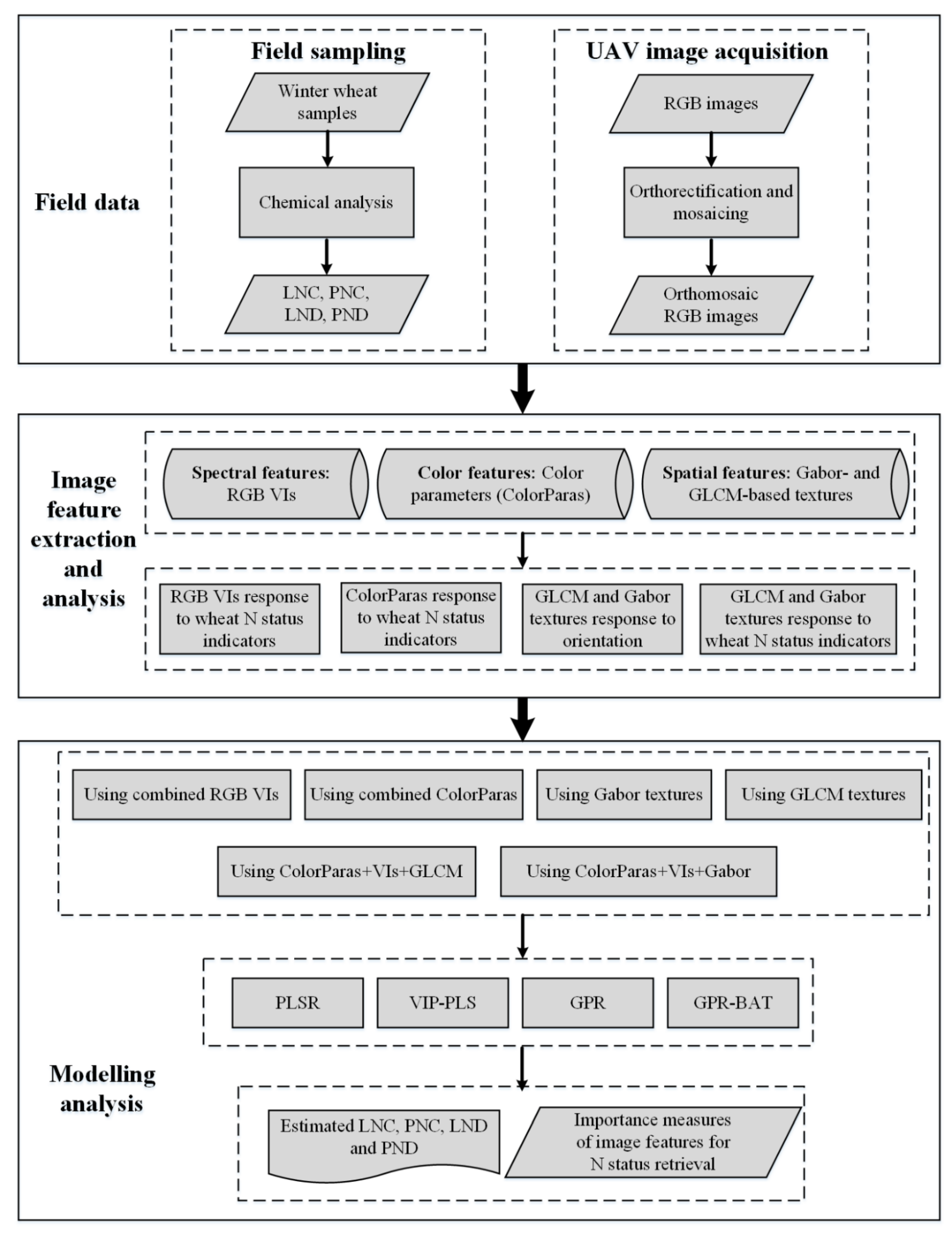
2. Materials and Methods

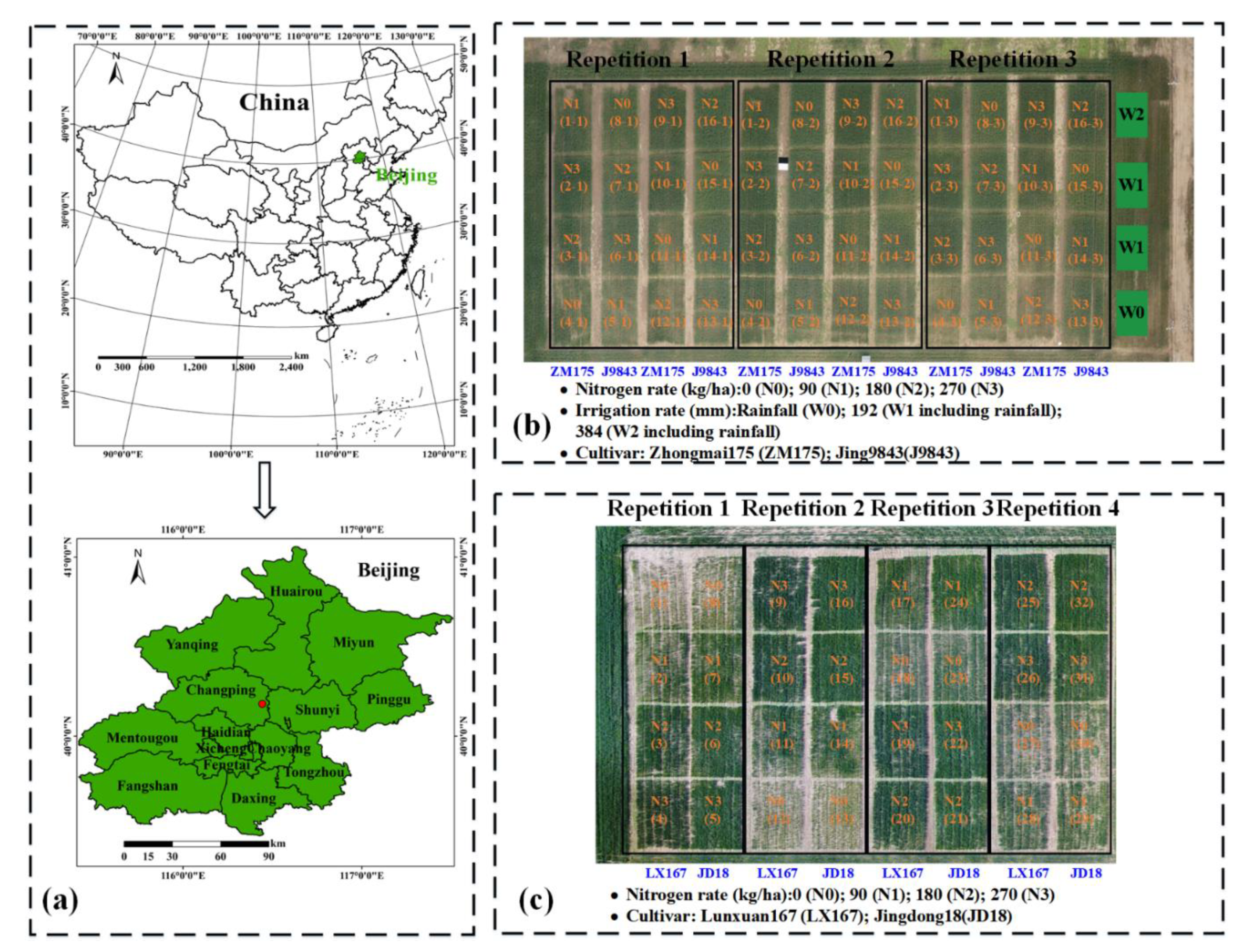
2.1. Experimental Design

The study site is located in the National Demonstration Research Base of Precision Agriculture (latitude 40°10′31′′ N to 40°11′18′′ N, and longitude 116°26′10′′ E to 116°27′05′′ E), Changping district, Beijing, China (Figure 1a). The climate of this experimental site is defined as a warm temperate, semi-humid continental monsoon climate. The temperature can reach up to 40 °C in summer, while the temperature in winter can reach as low as −10 °C. The average annual precipitation is approximately 450 mm. The experimental design in the 2014–2015 growing season was orthogonal, with three replications of two winter wheat varieties, four N fertilizer rates, and three irrigation levels (Figure 1b). There were 48 sample plots and each covered an area of 48 m2. The experiment in the 2018–2019 growing season was conducted with a completely randomized design, with four replications of two winter wheat cultivars and four N fertilizer application rates (Figure 1c). There were 64 sample plots and each covered an area of 135 m2. The irrigation management was the same for each sample plot in this experiment. For the two experiments, half of the nitrogen fertilizer was applied during plowing and the remaining fertilizer was applied at the jointing stage of winter wheat, along with irrigation. The other field management procedures, including pesticide and herbicide control and phosphate and potassium fertilizer, followed the standard practices for winter wheat production in this region.

2.2. Data Collection

2.2.1. UAV RGB Imagery Acquisition and Pre-Processing

For the experiments in the 2014–2015 growing season, an eight-rotor UAV (DJI S1000, SZ DJI Technology Co., Ltd., Shenzhen, China) was employed as the low-altitude remote sensing platform in this study. Equipped with a GPS sensor and two 18,000 mAh batteries, the UAV platform could fly automatically for about 20 min on the planned flight route, with a maximum take-off weight of 6 kg. A high-definition digital camera (Sony DSC-QX100, Sony, Tokyo, Japan) was attached to the UAV on a gimbal for RGB imagery acquisition. The RGB camera employs a 20.2-megapixel CMOS sensor with a 64-degree field-of-view lens. For the experiments in the 2018–2019 growing season, a four-rotor UAV called DJI Phantom 3 with a built-in RGB camera (12 megapixel) was used to capture wheat imagery. Ground and UAV field campaigns were conducted at winter wheat critical growth stages, including stem elongation (14 April 2015 and 16 April 2019, Zadoks growth stage (Z.S.) 31), booting (26 April 2015 and 30 April 2019, Z.S. 47), and anthesis (12th May 2015, Z.S. 65). The flight paths were designed by the DJI ground station, with a flight altitude of about 50 m and an intended forward overlap of 80% and side overlap of 75%. To guarantee the quality of acquired imagery, all flight missions proceeded between 10:00 and 14:00 (Beijing local time) and under stable light conditions. The camera settings, including the focal length, exposure time, aperture, and ISO, were adjusted to the lighting conditions for each flight.
The raw images were imported to Agisoft PhotoScan Pro (Version 1.4.2, Agisoft LLC., Russia) to generate ortho-rectified and geo-referred mosaic images based on the structure from motion algorithm and a mosaic blending model [27,28]. The main steps consisted of raw image sequence importing, image alignment, dense point cloud generation, mesh building, texture construction, and orthomosaic image generation. The ground sampling distance (GSD) of the orthomosaic images ranged from 0.90 to 1.11 cm. Relative radiometric correction described in [29] was conducted to maintain radiometric consistency in the case of multi-temporal remote sensing images. Then, the images were resampled to 1 cm using the nearest-neighbor method. To further reduce the impact of illumination changes, the normalization method described in [30] was carried out by dividing each pixel value of each band by the corresponding total intensity value of three bands. An area of interest (AOI) was delineated for each sample plot within the orthomosaic image to exclude the border effect. A total of 208 winter wheat AOIs (144 AOIs in 2015 and 64 AOIs in 2019) were clipped for the subsequent analysis.

2.2.2. Field Data Acquisition

After flight missions, ground destructive sampling was undertaken by randomly clipping a 0.25 m2 area of winter wheat in each plot at ground level. Twenty representative wheat tillers were randomly selected from the cut plants and then separated into leaves, stems, and ears. All plant samples were oven-dried at 105 °C for 30 min and then at 80 °C until a constant weight, in order to measure the biomass (dry matter, g/m2) of individual components. The dried plant components were milled and passed through a 1-mm sieve for Kjeldahl-N determination of each wheat component. The leaf N density (LND, g/m2), plant N density (PND, g/m2), plant N concentration (PNC, %), and aboveground biomass (AGB, g/m2) were calculated by the following Equations (1)–(4):
LND   =   LNC × LDM ,
PND   =   LNC × LDM + SNC × SDM + ENC × EDM ,
AGB   =   LDM + SDM + EDM ,
PNC   =   LNC × LDM + SNC × SDM + ENC × EDM AGB ,
where LNC, SNC, and ENC are the leaf N concentration (%), stem N concentration (%), and ear N concentration (%), respectively, and LDM, SDM, and EDM represent the leaf dry matter (g/m2), stem dry matter (g/m2), and ear dry matter (g/m2), respectively. At the growth stages of stem elongation and booting, the calculation of PNC, AGB, and PND did not involve wheat ear parameters since wheat ears were not formed during that time.

2.3. RGB Image Feature Extraction and Analysis

2.3.1. Spectral Features: RGB-Based VIs

A number of RGB-based VIs related to the crop growth status were selected from the literature (Table 1). For each winter wheat AOI, the average pixel values of each image channel were calculated, and RGB-based VIs were then computed for the subsequent analysis. Before assessing the predictability of RGB-based VIs, Pearson correlation analyses of these VIs and winter wheat N status indicators were conducted for multiple growth stages using a calibration dataset.

2.3.2. Color Features: Color Parameters from Different Color Space Models

The winter wheat AOIs were converted from an RGB color space model to other color space models, including HSV, L*a*b*, L*c*h*, and L*u*v* [30,41,42]. Table 2 summarizes the definition and conversion function of each color parameter in the five color space models. The mean pixel value of each color parameter was used for the subsequent analysis. Before assessing the predictability of color parameters, Pearson correlation analyses of these color parameters and winter wheat N status indicators were conducted for multiple growth stages using a calibration dataset.

2.3.3. Spatial Features: Gabor- and GLCM-Based Textures

Two types of image textural features were extracted, including Gabor-based textures and GLCM-based textures, for winter wheat N status estimation. In this study, eight GLCM-based textures were used, including the mean (Mean), variance (Var), homogeneity (Hom), contrast (Con), dissimilarity (Dis), entropy (Ent), second moment (Sec), and correlation (Cor) [43]. The GLCM-based textures were extracted from each band at four orientations with one pixel offset ([0, 1], [1, 1], [0, 1], [1, −1]). The size of the moving window during the calculation was set to 5 × 5, since it had a small influence on the texture metrics extracted from UAV-based RGB images with an ultrahigh spatial resolution (Yue et al., 2019). Finally, a total of 96 GLCM-based textures were extracted for each AOI. The suffixes “-R”, “-G”, and “-B” following the names of textures represented the GLCM-based textures from different bands (e.g., “Con-R” represents the contrast from the R band).
Two-dimension (2D) Gabor filters, which resemble a human visual system, have been prevalently used in image texture extraction [44]. They can capture image local directional features at multiple scales and thus, the extracted textural features are less sensitive to illumination variations [45]. A 2D Gabor filter is a product of a Gaussian function and a complex plane wave and can be defined as follows [46]:
Ψ μ , v ( z )   =   k μ , v 2 σ 2 e ( k μ , v 2 z 2 / 2 σ 2 ) [ e izk μ , v e σ 2 / 2 ] ,
where z = (x,y) denotes the pixel; µ and ν represent the orientation and scale of the Gabor filter, respectively;   σ is the ratio of the Gaussian window width and wavelength; k μ , v is the wave vector and equal to   k v e i μ , in which k ν   =   k m a x / f v and Φ µ   =   π µ / 8 ; k m a x is the maximum frequency; f is the spacing factor between filters in the frequency domain; and‖.‖denotes the norm operator [47].
In practice, a Gabor filter bank is generated by scaling and rotating the wave vector k μ , v . We considered four orientations of 0, π/4, π/2, and 3π/4; five scales (i.e., ν∈[0, 1, 2, 3, 4]); and a Gabor filter size of 5 × 5. The σ , k m a x , and f were set to π, π/2, and 2 , respectively. A total of 20 Gabor filters were constructed. After convoluting each channel of the RGB images with the Gabor filter bank, sixty Gabor textural images known as Gabor magnitude images were obtained. To reduce the dimension of the Gabor textural features, four descriptors, including the mean (GTmean, Mea), standard deviation (GTstd, Std), energy (GTenergy, Ene), and entropy (GTentropy, Ent), were calculated for each Gabor texture image, according to Equations (6)–(9) [48]:
G T m e a n   =   1 m n i   =   1 m j   =   1 n | g t i j | ,
G T s t d   =   1 m n i   =   1 m j   =   1 n ( g t i j G T m e a n ) 2 ,
G T e n e r g y   =   1 m n i   =   1 m j   =   1 n | g t i j | 2 ,
G T e n t r o p y   =   1 m n i   =   1 m j   =   1 n g t i j ( l o g ( g t i j 2 ) ) ,
where the size of a Gabor texture image is m × n and g t i j is the pixel value of a Gabor texture image at location (i,j). Finally, a total of 240 Gabor textural features were extracted from each winter wheat AOI for the subsequent analysis. To facilitate illustration hereafter, the letter indicating the feature scale and the letter “-R”, “-G” or “-B” (for R, B, and B bands, respectively) were used to differentiate the textures from different scales and bands. For example, “Mea-S1-R” represents the mean from the R band and scale 1, “Ene-S5-B” represents the energy from the B band and scale 5, and “Ent-S3-G” represents the entropy from the G band and scale 5, etc. Before analyzing the relationship between image textures and wheat N status indicators, the Gabor- and GLCM-based textures from each orientation were examined to determine whether there was heterogeneity in the textures of different orientations.

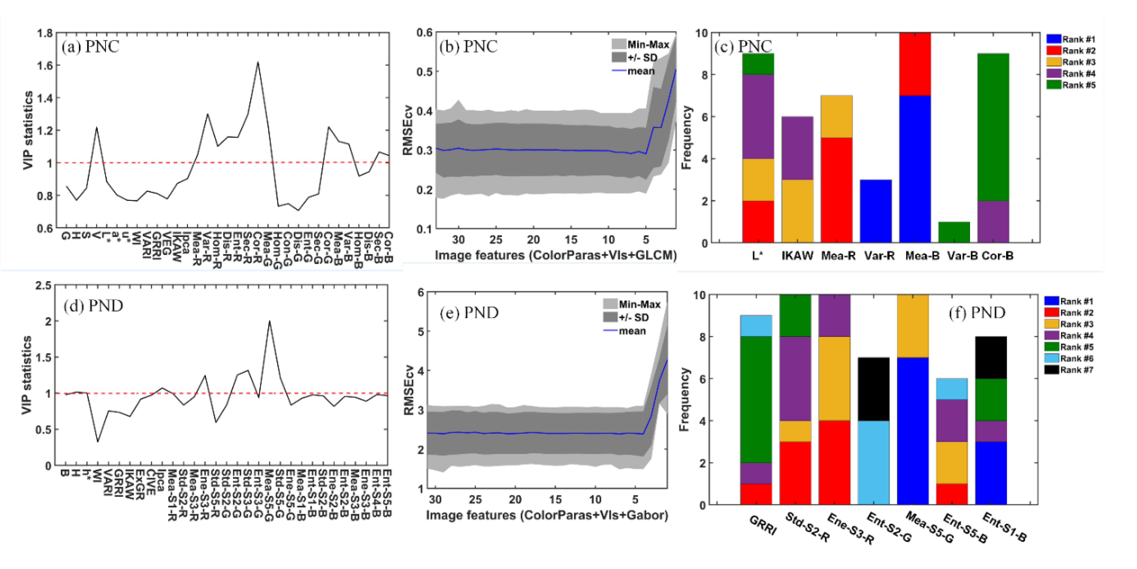
2.4. Identification of Influential Image Features and Modeling for Winter Wheat N Status Estimation

To understand which image features would be effective for winter wheat N status estimation, the band analysis tool (BAT) based on GPR (GPR-BAT) was used to identify influential image features during the development of models for each N status indicator of interest. Partial least square regression (PLSR) is one of the most frequently used linear nonparametric regression methods, due to its capability in dealing with multi-collinearity of input features, model interpretability, and computational performance [49]. The variable importance in projection (VIP) scores derived from PLSR can also reveal the features that contribute most to the response of interest. Therefore, PLSR and VIP-PLSR analyses were employed as benchmarks for comparisons with other methods used in this study.

2.4.1. PLSR Modeling and VIP-PLS

PLSR is one of the most popular multivariate statistical techniques applied to analyze data with a large number of collinear and noisy variables. It aims to decompose independent predictors into a set of orthogonal latent factors that maximize the covariance between predictors and responses [50]. The leave-one-out cross-validation method was used to determine the optimal number of factors in the PLSR model. To avoid under-fitting or over-fitting problems, the addition of an additional factor to the model required that it decreased the root mean square error of cross-validation by >2% [51,52]. A theoretical description of the PLSR technique was presented by Geladi and Kowalski and Wold et al. [49,50]. For a given PLSR model, the VIP scores for each image feature are computed as the weighted sum of squares of the PLS coefficients that take into account the amount of explained response variance in each latent factor [53]. The VIP scores offer a useful measure for identifying the image features which contribute the most to the winter wheat N status. Since the average of the squared VIP scores equals 1, the image features with VIP scores greater than 1 are considered significant for winter wheat N status estimation [54]. The VIP score of the jth image feature ( V I P j ) is calculated by Equation (10):
V I P j   =   p k   =   1 h ( S S Y k W k 2 ) / k   =   1 h S S Y c u m ,
where p is the number of predictors (image features); h is the number of components (latent factors); the term S S Y k is the variance of the sum of squares of Y explained by the component k; the term S S Y c u m is the total explained sum of squares; and W k 2 is the importance of the predictor in the component k.

2.4.2. GPR Modeling and GPR-BAT

GPR is a nonparametric machine learning regression approach, which learns the relationship between independent variables (e.g., image features) and dependent variables (e.g., N status indicators) by fitting a flexible probabilistic Bayesian model [25]. The use of a flexible kernel function (covariance function) generally suffices for tackling most regression problems and is beneficial if prior knowledge is weak [26]. Compared to other machine learning regression approaches, the parameter optimization of GPR is simpler and can be automatically completed by maximizing the marginal likelihood in the training set [55]. The convenient inference of GPR model parameters allows the relative contribution of each image feature to be evaluated by including a parameter per image feature, as in the anisotropic squared exponential kernel function (Equation (11)) [55]:
K ( X i , X j )   =   γ exp ( b   =   1 B ( x i b x j b ) 2 / 2 σ b 2 ) ,
where x i b represents the bth feature of the input feature vector X i ; γ is a scaling factor; and σ b is the dedicated parameter for controlling the spread of the relations for each image feature b (b = 1, …, B). The inverse of σ b represents the importance of the bth image feature to the GPR model. A smaller value of σ b indicates a higher level of informative content of this certain image feature. Verrelst et al. [55] integrated this property and sequential backward band removal (SBBR) as a new feature selection algorithm, in which the least significant feature with the highest σ b was removed at each iteration and a new GPR model was retrained with the remaining features only. To enable the automated identification of the best performing features for any regression problem, they integrated and automated this feature selection algorithm into a user-friendly tool named GPR-BAT [55].

2.5. Modeling Strategy and Statistical Analyses

The data from repetition 2 and repetition 3 collected in 2015 and the data from repetition 1, repetition 2, and repetition 3 collected in 2019 were used to calibrate the predictive models, and the remaining data were employed to validate the predictive models. Figure 2 illustrates the flowchart of this study, including data acquisition and processing, multiple image feature extraction and analysis, and model establishment and comparison. For each winter wheat N status indicator, PLSR and GPR analyses based on the combination of RGB-based VIs or the combination of color parameters were conducted to ascertain whether the combination could improve the estimation accuracy. To validate the effectiveness of Gabor-based textures in winter wheat N status estimation, PLSR and GPR analyses based on the Gabor-based textures and GLCM-based textures were conducted and compared. In the study, the combination of multiple image features indicated that one type of the two textural features, RGB-based VIs, and color parameters were concatenated, leading to an independent variable vector. For example, after Gabor-based textures of a certain orientation, all RGB-based VIs and color parameters are combined, and the resulting independent variable vector has 89 elements, consisting of 60 elements derived from Gabor-based textures, 16 elements derived from RGB-based Vis, and 13 elements derived from color parameters. The function “findCorrelation” in the “Caret” package was used to remove redundant image features before modeling. The cutoff value of this function was set to 0.99 in the study. To avoid the influence of inconsistent magnitudes of features, the feature combinations were standardized before PLSR and GPR analyses. The predictive performance of each model was evaluated with the coefficient of determination (R2val), root mean squared error (RMSEval, Equation (12)), and ratio of prediction to deviation (RPDval, Equation (13)).
R M S E v a l   =   i = 1 n ( Y e s t Y o b s ) 2 / n ,
RPD v a l   =   SD / RMSE ,
where Yest and Yobs are the estimated and observed winter wheat N status indicators, respectively; n is the number of samples; and SD is the standard deviation of the observed winter wheat N status indicator. We followed the RPD classification of Chang et al. [56]: Those with RPD > 2.0 were considered to be good quantitative models; values between 1.4 and 2.0 indicated a satisfactory performance of the model, which could be improved by using different calibration techniques; and <1.4 indicated an unreliable model.

3. Results

3.1. Descriptive Statistics

The N status indicators (i.e., LNC, PNC, LND, and PND) under different applied N rates and irrigation treatments were compared through the least significant difference test (LSD) at the 95% level of significance. The analysis results indicated that there were significant differences in the N status indicators under different N treatments for the two experiments (p < 0.05). For the experiments in 2015, different irrigation treatments led to a statistically significant difference in the LND and PND (p < 0.05). There was a significant difference in the LND under different N and irrigation treatments, considering the interaction effect of them (p < 0.05). The descriptive statistics of winter wheat N status indicators exhibited a moderate degree of variation, with the coefficient of variation (CV (%)) being between 12.25% and 47.63% (Table 3). The variability of N status indicators in the calibration dataset is larger than that in the validation dataset. With an acceptable approximation, all of the N status indicators, except for the LNC for validation, were normally distributed, with kurtosis between −3 and 3. For each N status indicator, the minimal and maximal values observed in the dataset are also shown in Table 3, in order to facilitate the understanding of RMSE for validation.

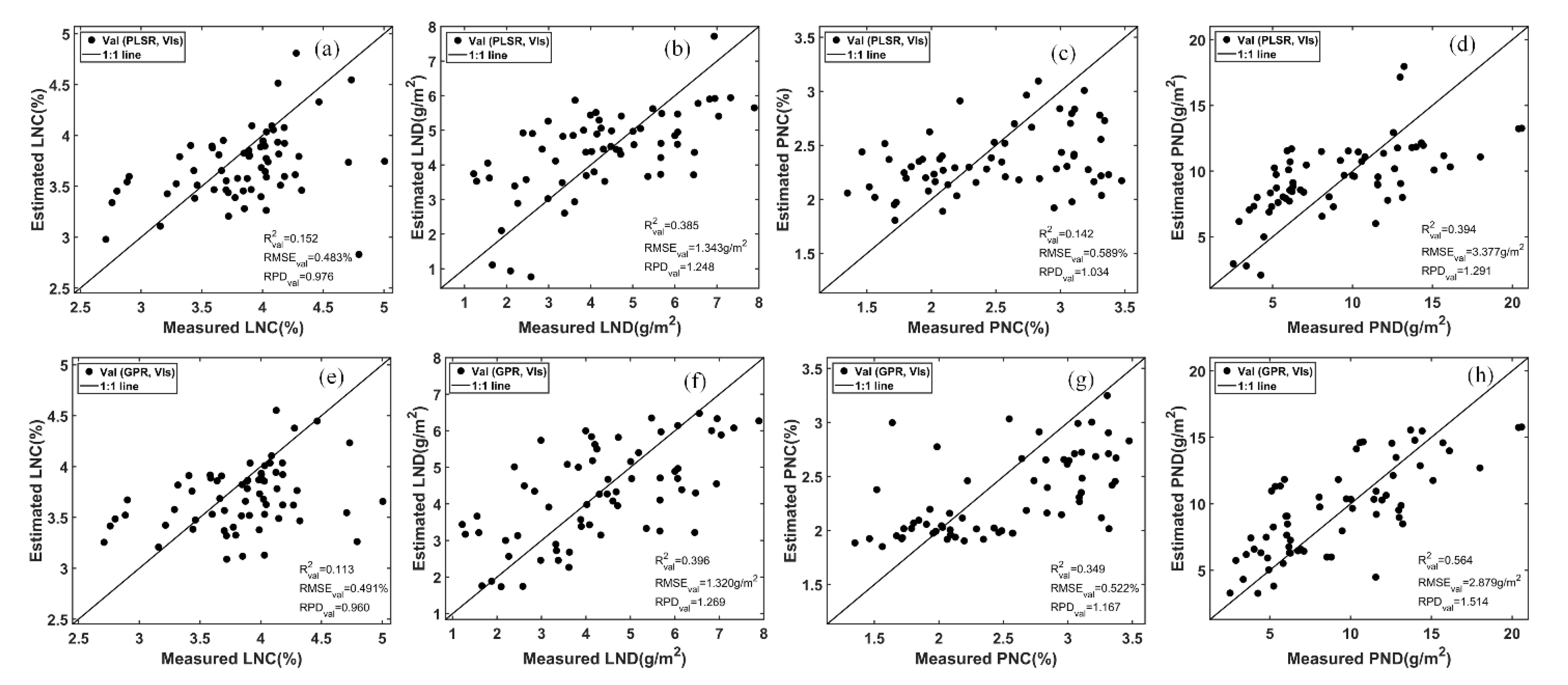
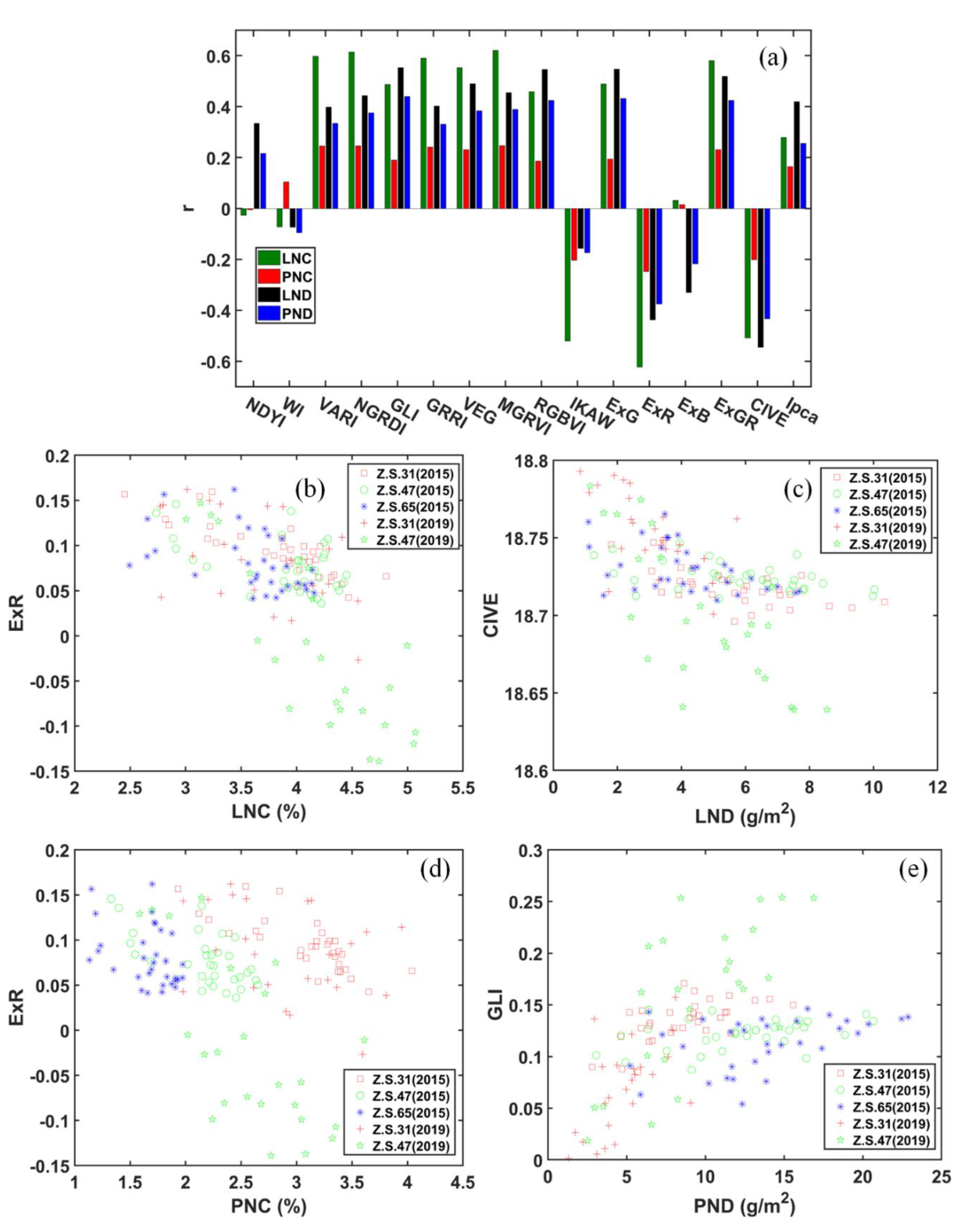
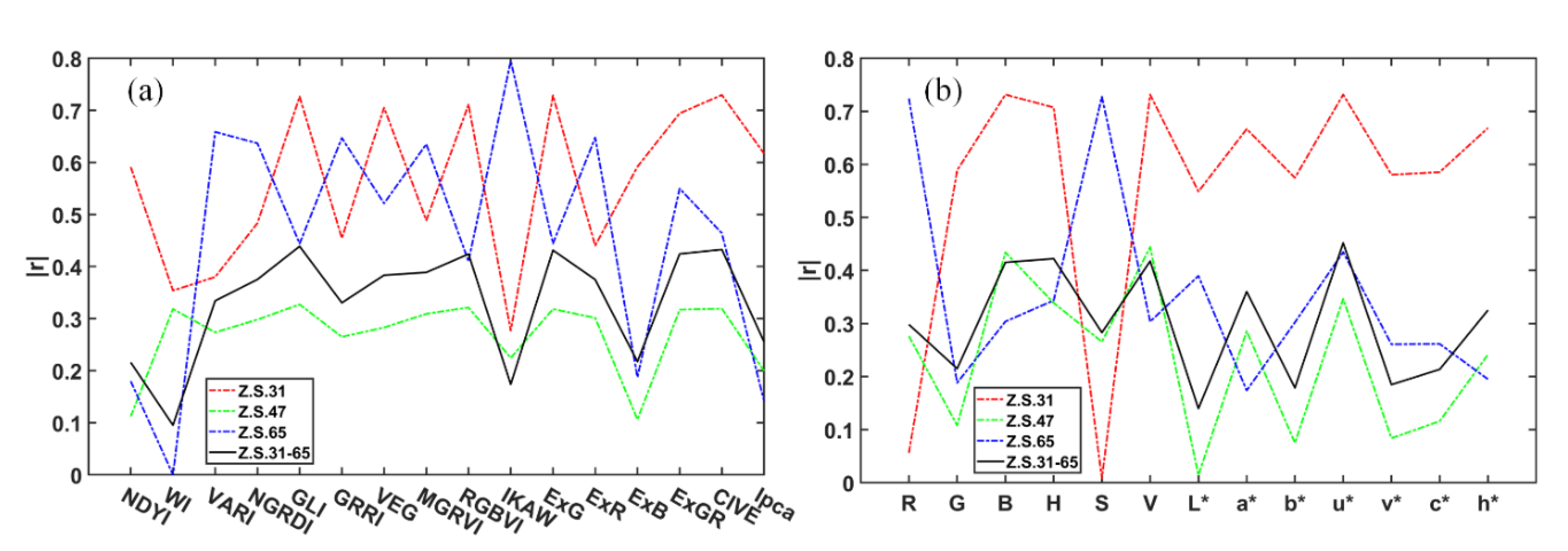
3.2. Using RGB-Based VIs to Estimate the Winter Wheat N Status

The Pearson correlation coefficients (r) between the RGB-based VIs and winter wheat N status indicators during multiple growth stages are shown in Figure 3a. It could be observed that the RGB-based VIs had a stronger correlation with LNC, LND, and PND than that with PNC. The highest correlation with PNC was produced by the ExG (r = −0.248, p < 0.01). Compared to the other RGB-based VIs, the Excess Green Vegetation Index (ExG), Colour Index of Vegetation Extraction (CIVE), and green leaf index (GLI) had a stronger correlation with LNC (r = −0.622, p < 0.01), LND (r = −0.545, p < 0.01), and PND (r = 0.439, p < 0.01), respectively. As can be observed from the scatter plots shown in Figure 3b–e, there were linear relationships between these best-performing VIs and N status indicators for each growth stage. However, the sensitivity of these VIs to the variation in N status indicators decreased when considering multiple growth stages. The analysis results indicated that relying on a single RGB-based VI could not produce reliable estimates of the winter wheat N status for multiple growth stages.
After removing highly correlated VIs, there were eight VIs left for the following modeling, including the normalized difference yellowness index (NDYI), Woebbecke index (WI), visible atmospherically-resistant index (VARI), green-red ratio index (GRRI), vegetative index (VEG), red green blue vegetation index (RGBVI), IKAW, and principal component analysis index (IPCA). As can be observed in Figure 4, both the PLSR and GPR models based on the combination of RGB-based VIs yielded higher estimation accuracies for the area-based N indicators (LND and PND) than those for the mass-based N indicators (LNC and PNC) (Figure 4). Among the models based on the combination of VIs, the GPR model for the PND estimation performed the best. Compared to the PLSR model, this model increased the R2val value by 0.17 and decreased the RMSEval value by 0.498 for the PND estimation. Apart from this GPR model, the RPD values for the other models were all lower than 1.4, indicating that these models could not produce reliable estimates of winter wheat N status indicators. In the comparison of Figure 4d,h, the saturation problem in the PND estimation was obviously alleviated after combining GPR and VIs. This indicated that the GPR method had advantages over PLSR in characterizing the nonlinear relationship between VIs and PND. However, for the other N status indicators, including LNC, LND, and PNC, the GPR models did not significantly improve the estimation accuracy more than the PLSR models did.

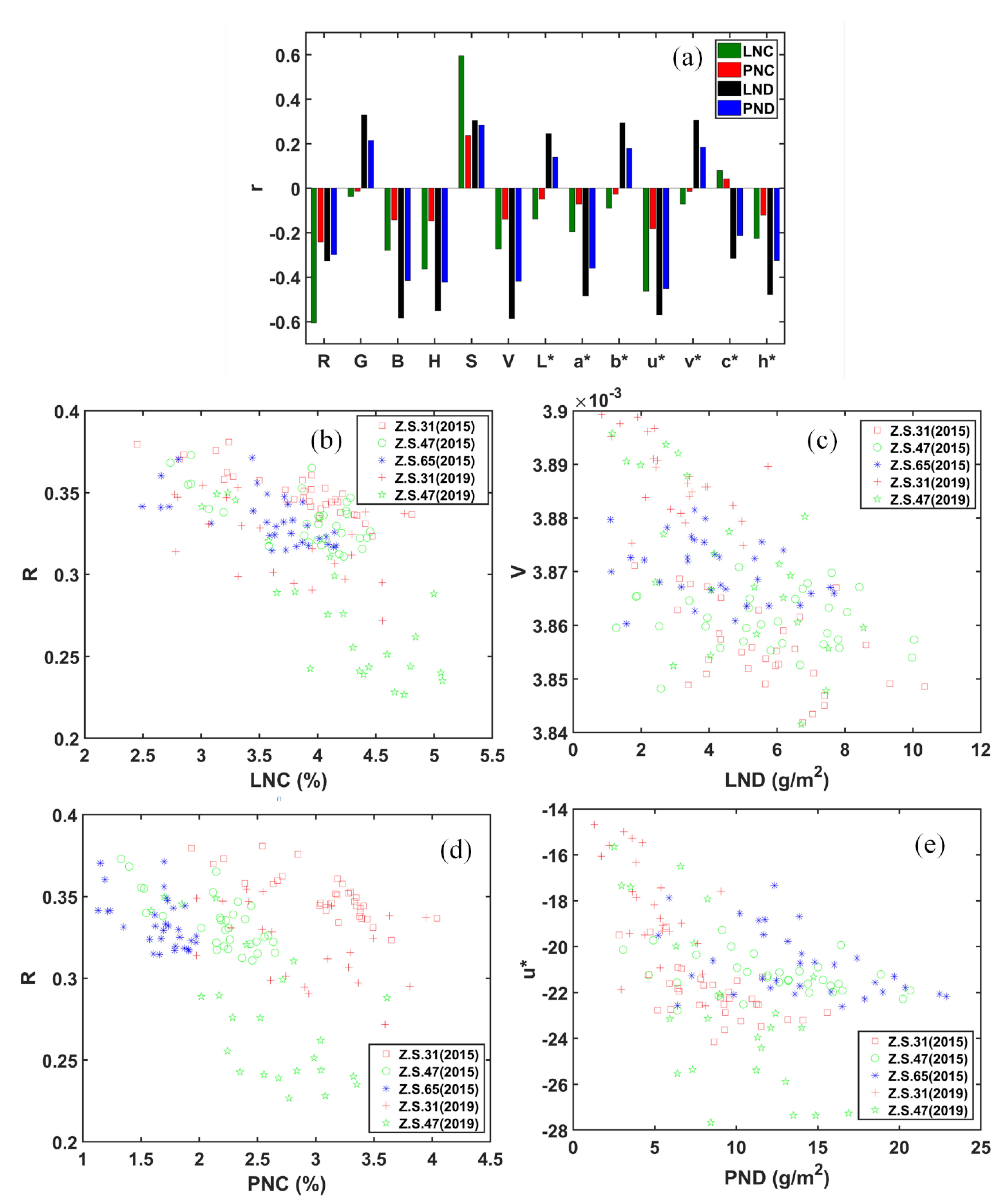
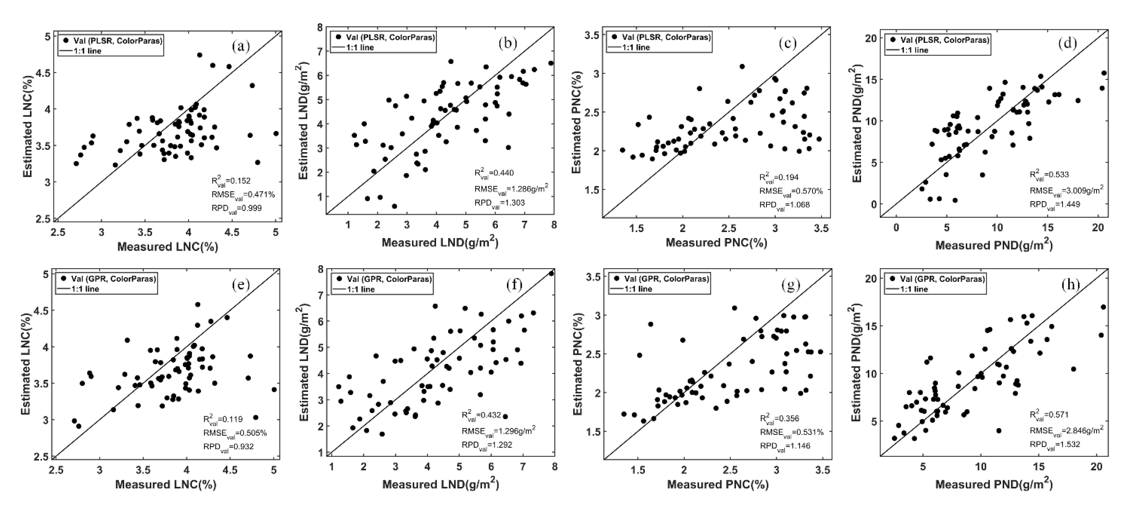
3.3. Using Color Parameters to Estimate the Winter Wheat N Status

The Pearson correlation coefficients for the color parameters and winter wheat N status indicators during multiple growth stages are shown in Figure 5a. Similar to the RGB-based VIs, the color parameters had a stronger correlation with LNC, LND, and PND than that with PNC. Among these color parameters, the color parameter R produced the highest correlation with LNC (r = −0.606, p < 0.01) and PNC (r = −0.242, p < 0.01), while the color parameters V and u* produced the highest correlation with LND (r = −0.586, p < 0.01) and PND (r = −0.452, p < 0.01), respectively. As can be observed from the scatter plots shown in Figure 5b–e, there was a linear relationship between these best-performing color parameters and N status indicators for each growth stage. However, the sensitivity of these color parameters to the N status indicators decreased when considering multiple growth stages. The analysis results demonstrated that accurate winter wheat N status estimates could not be obtained based on a single color parameter.
After removing highly correlated color parameters, there were six color parameters left for the following modeling, including H, S, V, L*, u*, and h*. Similar to the models based on the combination of VIs, both the PLSR and GPR models based on the combination of color parameters yielded higher estimation accuracies for the area-based N indicators (LND and PND) than those for the mass-based N indicators (LNC and PNC) (Figure 6). According to the RPD values of these models, only the PND could be reliably estimated. For the PND estimation, the predictive performance of the GPR model based on the combination of color parameters was similar to that of the GPR model based on the combination of VIs (Figure 4h and Figure 6h). Based on the combination of color parameters, the predictive performance of the GPR model for the PND estimation was better than that of the PLSR model (Figure 6d,h). However, the improvement was not as significant as that based on the combination of VIs after involving GPR.

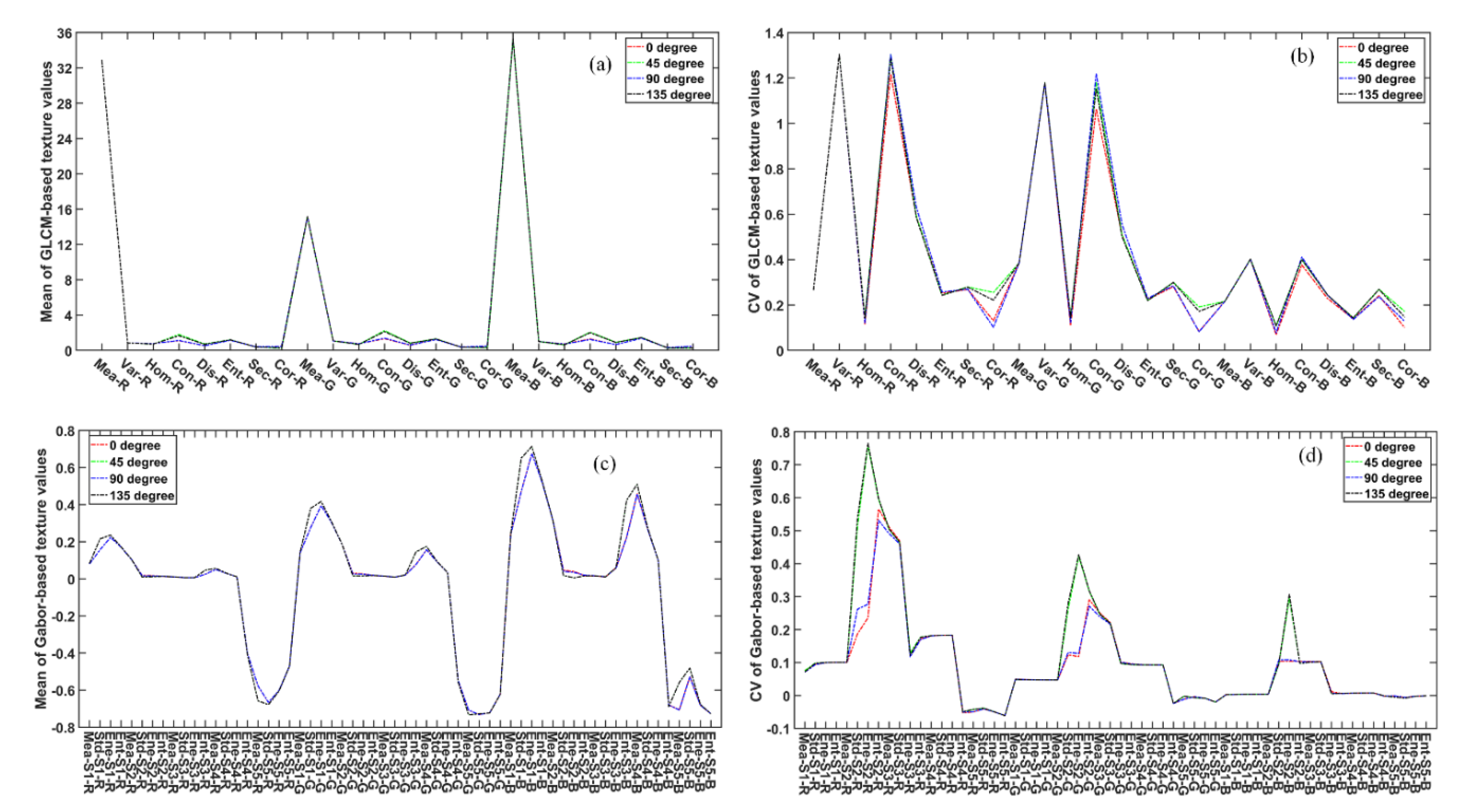
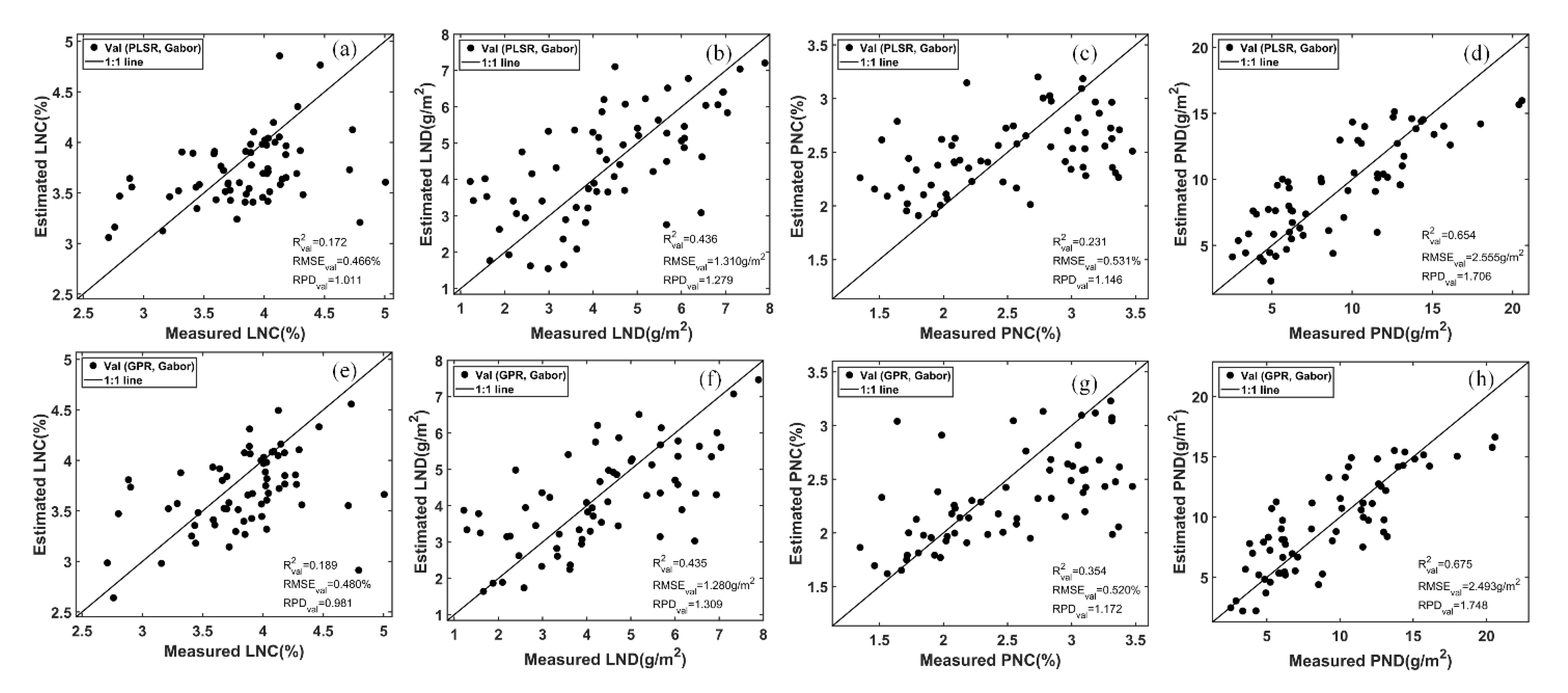
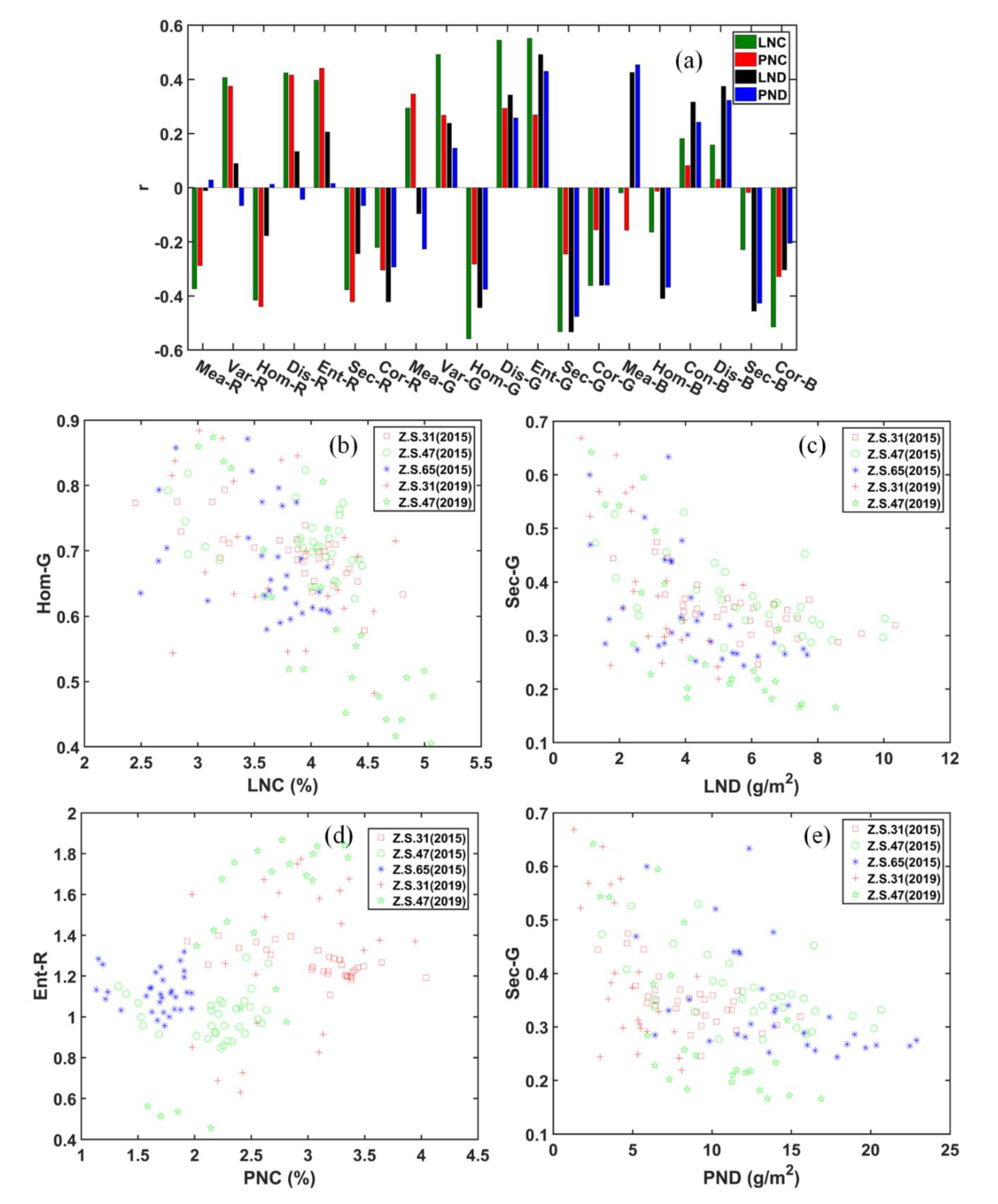
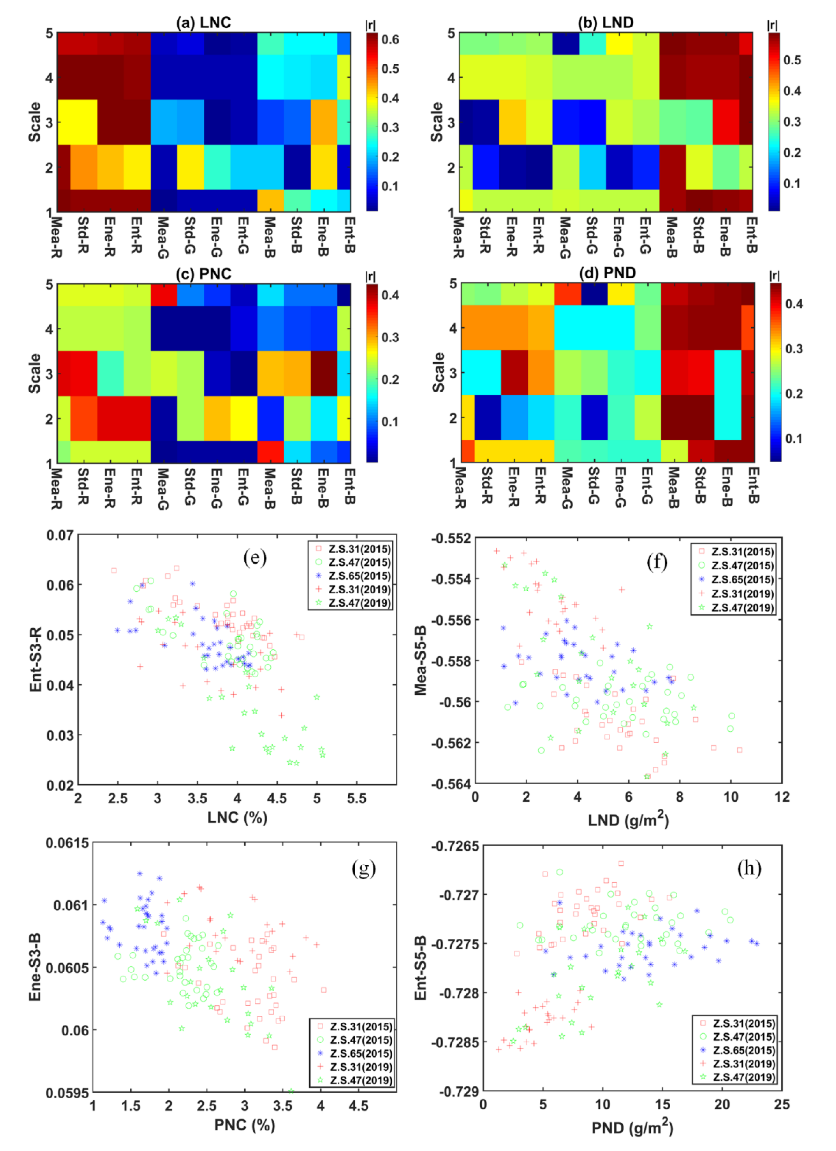
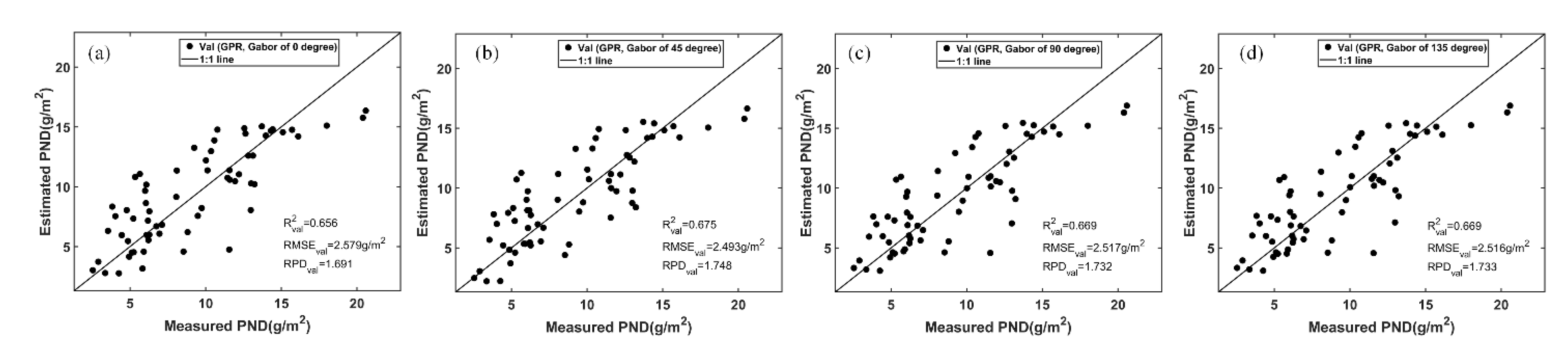
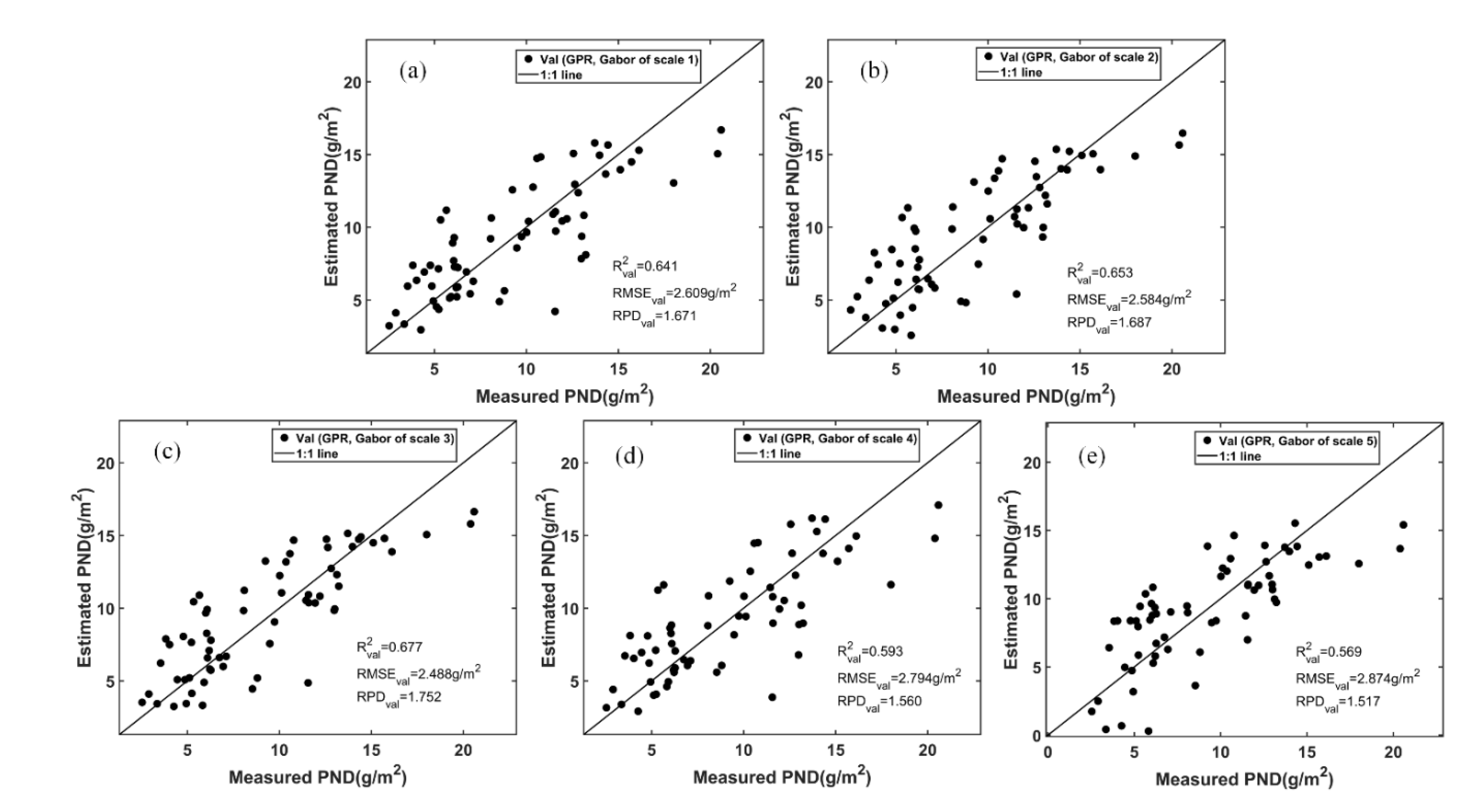
3.4. Using Gabor Textural Features to Estimate the Winter Wheat N Status

In this study, we extracted Gabor- and GLCM-based textural features with four orientations (i.e., 0°, 45°, 90°, and 135°). Based on the calibration dataset, the mean and coefficient of variation (CV) of these textures were calculated for each orientation to examine whether there was heterogeneity in the textures of different orientations. The approximately overlapped curves of the mean and CV indicated that both Gabor- and GLCM-based textures did not exhibit significant differences at different orientations for the winter wheat AOIs (Figure 7). However, the textures in the diagonal orientations (45°and 135°) showed a slightly higher degree of variation than the textures in the horizontal (0°) and vertical orientations (90°) (Figure 7b,d), especially for some Gabor-based textures. Therefore, the Gabor- and GLCM-based textures of 45° were used for the following analyses.
The Pearson correlation coefficients for the GLCM-based textures and winter wheat N status indicators during multiple growth stages are shown in Figure 8a. Compared to the RGB-based VIs and color parameters, the GLCM-based textures showed a higher correlation with PNC and PND, and the Ent-R and Sec-G produced the highest correlation with PNC (r = 0.441, p < 0.01) and PND (r = −0.476, p < 0.01), respectively. As can be observed from Figure 8b–e, the textures Ent-R and Sec-G stayed sensitive to the variation in PNC and PND during multiple growth stages, respectively. However, for the LNC and LND, the GLCM-based textures did not exhibit any advantages over VIs and color parameters. Therefore, the models based on the GLCM-based textures might be more promising than those on the combination of VIs or color parameters for the PNC and PND estimation. A similar tendency was observed in the correlation analyses of the Gabor-based textures and N status indicators (Figure 9). Among the Gabor-based textures, the Ene-S3-B and Ent-S5-B produced the highest correlation with PNC (r = −0.424, p < 0.01) and PND (r = 0.444, p < 0.01), respectively. The Gabor-based textures correlated well with N status indicators distributed at each scale (Figure 9a–d), so it was necessary to conduct multiscale analysis when using Gabor-based textures to estimate the winter wheat N status.
After removing redundant textures, there were 20 GLCM-based textures and 19 Gabor-based textures left for the subsequent analyses (Table 4). Similar to the models based on the combination of VIs or color parameters, the models based on the image textures (i.e., GLCM- and Gabor-based textures) did not yield reliable estimates of LNC and LND (Figure 10 and Figure 11). Among these models, the PLSR model based on the GLCM-based textures produced the highest estimation accuracy of PNC, with R2val = 0.612, RMSEval = 0.380%, and RPDval = 1.601 (Figure 10c). The GPR model based on the Gabor-based textures produced the highest estimation accuracy of PND, with R2val = 0.675, RMSEval = 2.493 g/m2, and RPDval = 1.748 (Figure 11h). The use of image textures significantly improved the estimation accuracies of PNC and PND. However, for the estimation of LNC and LND, these textural feature-based models only yielded slightly better or comparable results compared with the models using VIs or color parameters.

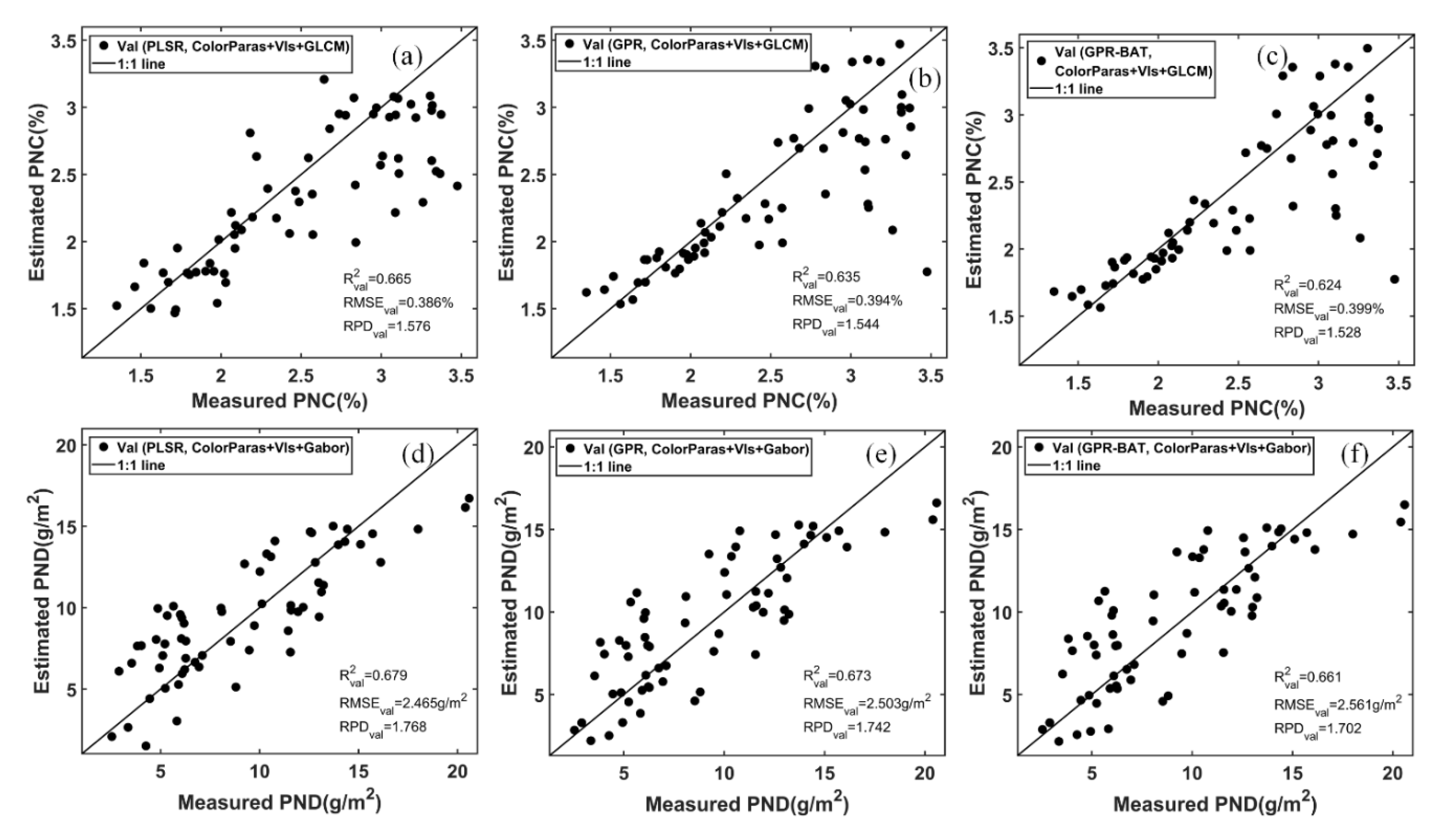
3.5. The Combined Use of RGB-Based VIs, Color Parameters, and Textures for Winter Wheat N Status Estimation

After removing highly correlated image features, there were 33 and 31 features left for the PNC and PND estimation, respectively (see the label of the horizontal axis of Figure 13a,d). With the combinations of textures, RGB-based Vis, and color parameters, the PLSR, GPR, and GPR-BAT analyses produced generally similar results to those with the textures alone. Among these models, the PLSR model based on the combination of GLCM-based textures, Vis, and color parameters yielded the highest estimation accuracy of PNC, with R2val = 0.665, RMSEval = 0.386%, and RPDval = 1.576 (Figure 12a). The PLSR model based on the combination of Gabor-based textures, Vis, and color parameters produced the highest estimation accuracy of PND, with R2val = 0.679, RMSEval = 2.465g/m2, and RPDval = 1.768 (Figure 12d). Figure 13a,d presents the VIP values of the image features used in the PLSR analyses for the PNC and PND estimation. It can be seen that the image textures notably had the highest VIP values. Ten-fold cross-validation was used in the GPR-BAT procedure. The averaged RMSEcv results, along with the standard deviation and min-max extremes, of the GPR models for the PNC and PND estimation are provided in Figure 13b,e. According to the two figures, the optimal number of image features involving the GPR-BAT models could be determined. For the PNC estimation, the optimal feature number was 7 and the selected features were L*, IKAW, Mea-R, Var-R, Mea-R, Var-B, and Cor-B. For the PND estimation, the optimal feature number was 7 and the selected features were GRRI, Std-S2-R, Ene-S3-R, Ent-S2-G, Mea-S5-B, Ent-S5-B, and Ent-S1-B. As shown in Figure 12c,f, the GPR-BAT models using the seven selected features yielded comparable estimation results to the GPR models using all image features. Figure 13c,f show the frequency of the selected image features for the PNC and PND estimation during the GPR-BAT procedure. It could be observed that textures were repeatedly selected as important predictors for the establishment of PNC and PND estimation models. For example, the textures Mea-B and Mea-S5-G appeared in the top three ranked features with a rather high frequency. Both the VIP-PLSR and GPR-BAT analyses indicated that image textures played an important role in the PNC and PND estimation of winter wheat.

4. Discussion

In this study, various water and N-fertilization treatments in winter wheat were conducted to represent the reality, which resulted in different winter wheat N nutrition statuses (Table 3). The consumer-grade digital camera deployed on the UAV platform was used to acquire winter wheat RGB imagery with an ultrahigh spatial resolution during critical growth stages of winter wheat. It allowed a thorough assessment of the utility of UAV-based RGB imagery in estimating mass- and area-based N status indicators of winter wheat. A comparison of the predictive performances of the image features from different feature spaces (namely, RGB-based VIs, color parameters, and textures) was also possible.

4.1. Limitations of RGB-Based VIs and Color Parameters in Wheat Winter N Status Estimation

In the correlation analyses of RGB-based VIs and winter wheat N status indicators, the RGB-based VIs, including ExR, CIVE, GLI, MGRVI, and ExGR, showed a relatively high correlation with the PND of winter wheat. The results are in agreement with the study of Yang et al. [16]. The Ipca did not show superiority to the other VIs in the correlation analyses with LNC (r = 0.279, p < 0.01). This result is not consistent with that observed in the study of Saberioon et al. [11]. Their findings indicated that Ipca could provide an indirect assessment of the rice leaf N status for all growth stages at both a leaf and canopy scale. This is mainly due to the fact that the construction of Ipca relies heavily on the site-specific dataset, thereby leading to poor generalization. In the correlation analyses of color parameters and winter wheat N status indicators, the color parameters V and u* negatively correlated with LND and PND, respectively. According to the definition, the color parameter V represents lightness, while the positive (or negative) u* represent redness (or greenness) (Table 2). The primary reason for the results is that winter wheat crops with different N contents exhibit different lightness and greenness. Winter wheat crops with higher N contents generally appear with a darker green color, while N-deficient winter wheat crops exhibit a light green color. The color parameter R exhibited a stronger negative correlation with LNC and PNC compared to the other color parameters. The results are in agreement with the findings reported by Mercado-Luna et al. [57], who confirmed that the color parameter R was a good predictor of the plant N status.
For a single growth stage, there were obvious linear relationships between VIs and N status indicators. However, the sensitivity of these VIs to the variation in N status indicators decreased when multiple growth stages were considered (see Figure 14a, taking PND as an example). Apart from the influence of the growth stage, the RGB-based VIs also suffered from a saturation problem when estimating N status indicators. The RGB-based VIs were determined by the intensity values at two or three RGB image channels and sensitive to the amplitude of the reflectance intensity. However, the responses of the reflectance intensity in visible bands to the variation in wheat N content are very limited [58,59,60]. This results in RGB-based VIs asymptotically approaching a saturation level after the wheat N content exceeds a certain value (Figure 3). Therefore, using a single RGB-based VI does not produce competent data when estimating winter wheat N status indicators for multiple growth stages. The predictive performance of color parameters was also impeded by the growth stage and saturation problem (Figure 5 and Figure 14b).
The combined use of RGB-based VIs produced higher estimation accuracies for the area-based N status indicators (LND and PND) than those for the mass-based N status indicators (LNC and PNC), whatever the linear (PLSR) or nonlinear (GPR) nonparametric regression method applied. Similar results were observed when using the combination of color parameters from different color space models. This might be partly attributed to the calculation principles for RGB-based VIs and color parameters. They were all derived from winter wheat canopy images, which consist of soils, shaded leaves, illuminated leaves, stems, and ears. From the jointing to heading and flowering stage, the canopy structure of winter wheat changes, thereby changing the proportions of these components. This means that both RGB-based VIs and color parameters not only contain information related to the reflectance intensity and color, but also contain partial information related to the canopy cover and aboveground biomass. According to the definition of area-based N status indicators, they are closely correlated with plant biomass. In this study, the aboveground biomass of winter wheat exhibited good correlations with LND and PND, with correlation coefficients of 0.415 and 0.873, respectively. This explains why the combined use of RGB-based VIs and color parameters could estimate area-based N status indicators well in comparison to the mass-based N status indicators. In addition, both RGB-based VIs and color parameters reflect more information about the winter wheat canopy as a whole, rather than just the leaves. Therefore, the use of RGB-based VIs and color parameters produced higher estimation accuracies for the PND than those for the LND (Figure 4 and Figure 6). For the PND estimation, the PLSR model based on the combination of color parameters achieved a comparable accuracy to the GPR model based on the combination of RGB-based VIs. This indicated that the color parameters were better linearly correlated with PND compared to the RGB-based VIs, which is mainly due to the fact that the color parameters from different color space models can provide various levels of information associated with the winter wheat canopy color, which might partly alleviate the saturation problem of RGB-based VIs. Nonetheless, the combined use of color parameters did not produce a better performance than the Gabor- and GLCM-based textures for the PND estimation. The soil background is an important influential factor in the crop canopy color in the transition from a leaf to canopy scale. Further study will explore how the soil background influences the relationship between color parameters and the wheat N status and whether removing the soil background can improve the performance of color parameters in wheat N status estimation.

4.2. Ability of Image Textures to Estimation the Winter Wheat N Status

Image textures have the ability to reflect dynamic changes of vegetation canopy cover and structure, and thus have been widely used in estimating vegetation biomass and the leaf area index (LAI) [22,23,61]. The amount of N uptake is an important inner driver of crop growth. Normally, crops with an adequate supply of N have a dark green color, and a large leaf area and crop population [62]. In contrast, N-deficient crops are often characterized by yellow and small leaves, and small crop populations [63]. Therefore, image textures have great potential in quantifying the crop N status. In the exploration of the applicability of the textures derived from UAV-based RGB images for the winter wheat N status estimation, the GLCM- and Gabor-based textures respectively produced higher accuracies for the estimation of PNC and PND compared to the RGB-based VIs and color parameters. However, these textures did not improve the estimations of LNC and LND, and only achieved comparable results to the combination of color parameters. It is important to note that the PLSR model based on the GLCM-based textures produced the highest accuracy for the estimation of PNC (Figure 10c). This might be attributed to the N dilution theory in which PNC decreases monotonically with an increasing plant dry biomass [64]. Yue et al. and Zheng et al. [22,65] have confirmed that the GLCM-based textures performed well for crop biomass estimation. Liu et al. [15] indicated that the GLCM-based textures improved the remote estimation of the nitrogen nutrition index (the ratio of critical PNC to biomass) in winter oilseed rape. However, the Gabor-based textures did not yield acceptable estimates of winter wheat PNC. The primary reason for the result is that the Gabor-based textures used in the study contain some color information, which is not conducive to PNC estimation (Figure 6c,g). The low-frequency parts of the Gabor-based textures are an approximation of the original RGB images at different scales. In contrast, the GLCM-based textures are derived from the graytone spatial-dependance matrix and represent the heterogeneity in the tonal values of pixels within an area of interest [43,66]. This means that the GLCM-based textures of winter wheat canopy images mainly capture the high-frequency information, representing flourishing crops [22].
For both Gabor- and GLCM-based textures, there was no significant heterogeneity in the textures of different orientations. This means that there is a little difference in the predictive performance of the textures of different orientations. This conclusion was confirmed by the similar estimation accuracy of PND produced by the Gabor-based textures of each orientation (Figure 15). In practical applications, the use of textures of 45° is recommended, since they exhibited a slightly higher degree of variation and produced a slightly better estimation accuracy (Figure 15). The Gabor-based textures of five scales were extracted in the study for the analyses. The scale values determine the frequency of Gabor filters. Since the spatial structure of the winter wheat canopy varies with growth stages, the frequency of the Gabor filter should vary in a range to cover the whole 2D image domain, obtaining sufficient discriminative features for subsequent analysis. Considering the estimation of PND as an example, Figure 16 displays the predictive performance of the GPR models based on the Gabor-based textures of each scale. It could be observed that the Gabor-based textures of scale 3 performed better than those of the other scales. However, the optimal scale for using Gabor-based textures to quantify the winter wheat N status depends on the crop canopy size and planting density. Before making the relationships between the optimal scale of the Gabor filter and canopy size and planting density clear, the use of multiscale Gabor-based textures is a wise choice for the estimation of the crop N status.
The combined use of RGB-based VIs, color parameters, and textures only produced comparable accuracies when using textures alone for the estimation of PNC and PND. There are two reasons for the results. First, the textures play an important role in the estimation of PNC and PND. This is confirmed by the analysis results of VIP-PLSR and GPR-BAT, which indicated that the textures were the features contributing the most for the estimation of PNC and PND. Second, the low-frequency parts of Gabor-based textures already contain partial information related to color and RGB-based VIs for the PND estimation. It is worth noting that the GPR-BAT models with just seven features exhibited comparable accuracies to those with all features for the estimation of PNC and PND. The feature selection function embedded in the GPR-BAT models helps identify the subset of important features which are correlated with winter wheat PNC and PND. It not only decreases the model complexity, but also enhances the model interpretability.

5. Conclusions

Nitrogen plays a significant role in many aspects of crop growth and development. Accurate estimates of the winter wheat N status are valuable for practicing precise farming. The UAV equipped with a low-cost RGB camera overcomes many problems associated with satellite and airborne remote sensing systems, and provides a cost-effective means for winter wheat N status monitoring. This study explored the feasibility of RGB-based VIs, color parameters, and textures derived from UAV-based RGB images for winter wheat N status estimation. Both mass- (i.e., LNC and PNC) and area-based (i.e., LND and PND) N status indicators were considered. The combined use of RGB-based VIs and color parameters could only produce reliable estimates of PND. The GPR model based on the Gabor-based textures yielded the highest estimation accuracy of PND, while the PLSR model based on the GLCM-based textures yielded the highest estimation accuracy of PNC. Both the analyses of VIP-PLSR and GRP-BAT indicated that textures were the features that contributed the most in the estimation of PNC and PND. GPR regression with the built-in feature selection function is a promising candidate for the implementation of winter wheat N status estimation. This study demonstrated the potential application of textural features derived from UAV-based RGB images for the estimation of PNC and PND in winter wheat. Our findings will serve as an informative guide on how to use the features derived from UAV-based RGB images for winter wheat N status estimation. However, further studies are recommended for predicting the crop N status under various ecological regions to dispatch this as a widespread technique in agricultural management.

Author Contributions

Conceptualization, Y.F.; methodology, Y.F.; software, Y.F.; validation, Y.F.; formal analysis, Y.F.; investigation, Y.F.; resources, Z.L. (Zhenhai Li); data curation, Z.L. (Zhenhai Li), X.X., and X.S.; writing—original draft preparation, Y.F.; writing—review and editing, Y.F. and G.Y.; visualization, Y.F.; supervision, G.Y., Z.L. (Zhenhong Li), and C.Z.; project administration, G.Y. and C.Z.; funding acquisition, Y.F, G.Y., P.W., and C.Z. All authors have read and agreed to the published version of the manuscript.

Funding

This study was supported by the National Key Research and Development Program of China (2016YFD0700303), the Natural Science Foundation of China (41801225), the Beijing Natural Science Foundation (6182011), the China Postdoctoral Science Foundation (2017M620675), the Beijing Postdoctoral Research Foundation, and the Postdoctoral Research Foundation sponsored by the Beijing Academy of Agriculture and Forestry Sciences.

Acknowledgments

The authors extend gratitude to Haikuan Feng, Bo Xu, Weiguo Li, and Hong Chang for their assistance in field data collection.

Conflicts of Interest

The authors declare no conflict of interest.

References

  1. Diacono, M.; Rubino, P.; Montemurro, F. Precision nitrogen management of wheat. A review. Agron. Sustain. Dev. 2013, 33, 219–241. [Google Scholar] [CrossRef]
  2. Ali, M.M.; Al-Ani, A.; Eamus, D.; Tan, D.K.Y. Leaf nitrogen determination using non-destructive techniques—A review. J. Plant Nutr. 2017, 40, 928–953. [Google Scholar] [CrossRef]
  3. Fu, Y.; Yang, G.; Li, Z.; Li, H.; Li, Z.; Xu, X.; Song, X.; Zhang, Y.; Duan, D.; Zhao, C.; et al. Progress of hyperspectral data processing and modelling for cereal crop nitrogen monitoring. Comput. Electron. Agric. 2020, 172, 105321. [Google Scholar] [CrossRef]
  4. Delloye, C.; Weiss, M.; Defourny, P. Retrieval of the canopy chlorophyll content from Sentinel-2 spectral bands to estimate nitrogen uptake in intensive winter wheat cropping systems. Remote. Sens. Environ. 2018, 216, 245–261. [Google Scholar] [CrossRef]
  5. Croft, H.; Arabian, J.; Chen, J.M.; Shang, J.; Liu, J. Mapping within-field leaf chlorophyll content in agricultural crops for nitrogen management using Landsat-8 imagery. Precis. Agric. 2019, 21, 856–880. [Google Scholar] [CrossRef] [Green Version]
  6. Moharana, S.; Dutta, S. Spatial variability of chlorophyll and nitrogen content of rice from hyperspectral imagery. ISPRS J. Photogramm. Remote. Sens. 2016, 122, 17–29. [Google Scholar] [CrossRef]
  7. Nigon, T.J.; Mulla, D.J.; Rosen, C.J.; Cohen, Y.; Alchanatis, V.; Knight, J.; Rud, R. Hyperspectral aerial imagery for detecting nitrogen stress in two potato cultivars. Comput. Electron. Agric. 2015, 112, 36–46. [Google Scholar] [CrossRef]
  8. Jin, X.; Zarco-Tejada, P.; Schmidhalter, U.; Reynolds, M.P.; Hawkesford, M.J.; Varshney, R.K.; Yang, T.; Nie, C.; Li, Z.; Ming, B.; et al. High-throughput estimation of crop traits: A review of ground and aerial phenotyping platforms. IEEE Geosci. Remote. Sens. Mag. 2020. [Google Scholar] [CrossRef]
  9. Yang, G.; Liu, J.; Zhao, C.; Li, Z.; Huang, Y.; Yu, H.; Xu, B.; Yang, X.; Zhu, D.; Zhang, X.; et al. Unmanned Aerial Vehicle Remote Sensing for Field-Based Crop Phenotyping: Current Status and Perspectives. Front. Plant Sci. 2017, 8, 1111. [Google Scholar] [CrossRef]
  10. Pagola, M.; Ortiz, R.; Irigoyen, I.; Bustince, H.; Barrenechea, E.; Aparicio-Tejo, P.; Lamsfus, C.; Lasa, B. New method to assess barley nitrogen nutrition status based on image colour analysis. Comput. Electron. Agric. 2009, 65, 213–218. [Google Scholar] [CrossRef]
  11. Saberioon, M.M.; Amin, M.S.M.; Anuar, A.R.; Gholizadeh, A.; Wayayok, A.; Khairunniza-Bejo, S. Assessment of rice leaf chlorophyll content using visible bands at different growth stages at both the leaf and canopy scale. Int. J. Appl. Earth Obs. Geoinf. 2014, 32, 35–45. [Google Scholar] [CrossRef]
  12. Zhang, M.; Zhou, J.; Sudduth, K.A.; Kitchen, N.R. Estimation of maize yield and effects of variable-rate nitrogen application using UAV-based RGB imagery. Biosyst. Eng. 2020, 189, 24–35. [Google Scholar] [CrossRef]
  13. Graeff, S.; Pfenning, J.; Claupein, W.; Liebig, H.-P. Evaluation of Image Analysis to Determine the N-Fertilizer Demand of Broccoli Plants (Brassica oleracea convar. botrytis var. italica). Adv. Opt. Technol. 2008, 2008, 359760. [Google Scholar] [CrossRef] [Green Version]
  14. Li, J.; Zhang, F.; Qian, X.; Zhu, Y.; Shen, G. Quantification of rice canopy nitrogen balance index with digital imagery from unmanned aerial vehicle. Remote. Sens. Lett. 2015, 6, 183–189. [Google Scholar] [CrossRef]
  15. Liu, S.; Li, L.; Gao, W.; Zhang, Y.; Liu, Y.; Wang, S.; Lu, J. Diagnosis of nitrogen status in winter oilseed rape (Brassica napus L.) using in-situ hyperspectral data and unmanned aerial vehicle (UAV) multispectral images. Comput. Electron. Agric. 2018, 151, 185–195. [Google Scholar] [CrossRef]
  16. Yang, B.; Wang, M.; Sha, Z.; Wang, B.; Chen, J.; Yao, X.; Cheng, T.; Cao, W.; Zhu, Y. Evaluation of Aboveground Nitrogen Content of Winter Wheat Using Digital Imagery of Unmanned Aerial Vehicles. Sensors 2019, 19, 4416. [Google Scholar] [CrossRef] [Green Version]
  17. Zhou, X.; Huang, W.; Kong, W.; Ye, H.; Luo, J.; Chen, P. Remote estimation of canopy nitrogen content in winter wheat using airborne hyperspectral reflectance measurements. Adv. Space Res. 2016, 58, 1627–1637. [Google Scholar] [CrossRef]
  18. Clevers, J.G.P.W.; Kooistra, L. Using Hyperspectral Remote Sensing Data for Retrieving Canopy Chlorophyll and Nitrogen Content. IEEE J. Sel. Top. Appl. Earth Obs. Remote. Sens. 2012, 5, 574–583. [Google Scholar] [CrossRef]
  19. Hunt, E.R.; Cavigelli, M.; Daughtry, C.S.; McMurtrey, J.E.; Walthall, C.L. Evaluation of Digital Photography from Model Aircraft for Remote Sensing of Crop Biomass and Nitrogen Status. Precis. Agric. 2005, 6, 359–378. [Google Scholar] [CrossRef]
  20. Kawashima, S. An Algorithm for Estimating Chlorophyll Content in Leaves Using a Video Camera. Ann. Bot. 1998, 81, 49–54. [Google Scholar] [CrossRef] [Green Version]
  21. Fu, Y.; Taneja, P.; Lin, S.; Ji, W.; Adamchuk, V.; Daggupati, P.; Biswas, A. Predicting soil organic matter from cellular phone images under varying soil moisture. Geoderma 2020, 361, 114020. [Google Scholar] [CrossRef]
  22. Yue, J.; Yang, G.; Tian, Q.; Feng, H.; Xu, K.; Zhou, C. Estimate of winter-wheat above-ground biomass based on UAV ultrahigh-ground-resolution image textures and vegetation indices. ISPRS J. Photogramm. Remote Sens. 2019, 150, 226–244. [Google Scholar] [CrossRef]
  23. Li, S.; Yuan, F.; Ata-Ul-Karim, S.T.; Zheng, H.; Cheng, T.; Liu, X.; Tian, Y.; Zhu, Y.; Cao, W.; Cao, Q. Combining Color Indices and Textures of UAV-Based Digital Imagery for Rice LAI Estimation. Remote Sens. 2019, 11, 1763. [Google Scholar] [CrossRef] [Green Version]
  24. Shen, L.; Bai, L. A review on Gabor wavelets for face recognition. Pattern Anal. Appl. 2006, 9, 273–292. [Google Scholar] [CrossRef]
  25. Camps-Valls, G.; Verrelst, J.; Muñoz-Marí, J.; Laparra, V.; Mateo-Jimenez, F.; Gomez-Dans, J. A Survey on Gaussian Processes for Earth-Observation Data Analysis: A Comprehensive Investigation. IEEE Geosci. Remote Sens. Mag. 2016, 4, 58–78. [Google Scholar] [CrossRef] [Green Version]
  26. Verrelst, J.; Alonso, L.; Camps-Valls, G.; Delegido, J.; Moreno, J. Retrieval of Vegetation Biophysical Parameters Using Gaussian Process Techniques. IEEE Trans. Geosci. Remote. Sens. 2012, 50, 1832–1843. [Google Scholar] [CrossRef]
  27. Verhoeven, G. Taking computer vision aloft-archaeological three-dimensional reconstructions from aerial photographs with photoscan. Archaeol. Prospect. 2011, 18, 67–73. [Google Scholar] [CrossRef]
  28. Brown, M.; Lowe, D.G. Recognising panoramas. In Proceedings of the Ninth IEEE International Conference on Computer Vision, Nice, France, 13–16 October 2003; Volume 2, pp. 1218–1225. [Google Scholar] [CrossRef]
  29. Yue, J.; Feng, H.; Jin, X.; Yuan, H.; Li, Z.; Zhou, C.; Yang, G.; Tian, Q. A Comparison of Crop Parameters Estimation Using Images from UAV-Mounted Snapshot Hyperspectral Sensor and High-Definition Digital Camera. Remote Sens. 2018, 10, 1138. [Google Scholar] [CrossRef] [Green Version]
  30. Cheng, H.; Jiang, X.; Sun, Y.; Wang, J. Color image segmentation: Advances and prospects. Pattern Recognit. 2001, 34, 2259–2281. [Google Scholar] [CrossRef]
  31. Woebbecke, D.M.; Meyer, G.E.; Von Bargen, K.; Mortensen, D.A. Color Indices for Weed Identification Under Various Soil, Residue, and Lighting Conditions. Trans. ASAE 1995, 38, 259–269. [Google Scholar] [CrossRef]
  32. Gamon, J.A.; Surfus, J.S. Assessing leaf pigment content and activity with a reflectometer. New Phytol. 1999, 143, 105–117. [Google Scholar] [CrossRef]
  33. Gitelson, A.A.; Kaufman, Y.J.; Stark, R.; Rundquist, D. Novel algorithms for remote estimation of vegetation fraction. Remote. Sens. Environ. 2002, 80, 76–87. [Google Scholar] [CrossRef] [Green Version]
  34. Mao, W.; Wang, Y.; Wang, Y. Real-time Detection of Between-row Weeds Using Machine Vision. In Proceedings of the 2003 ASAE Annual Meeting 2003, Las Vegas, NV, USA, 27–30 July 2003; p. 1. [Google Scholar] [CrossRef]
  35. Kataoka, T.; Kaneko, T.; Okamoto, H.; Hata, S. Crop growth estimation system using machine vision. In Proceedings of the 2003 IEEE/ASME International Conference on Advanced Intelligent Mechatronics (AIM 2003), Kobe, Japan, 20–24 July 2003; Volume 2, pp. b1079–b1083. [Google Scholar] [CrossRef]
  36. Hague, T.; Tillett, N.D.; Wheeler, H. Automated Crop and Weed Monitoring in Widely Spaced Cereals. Precis. Agric. 2006, 7, 21–32. [Google Scholar] [CrossRef]
  37. Meyer, G.E.; Neto, J.C. Verification of color vegetation indices for automated crop imaging applications. Comput. Electron. Agric. 2008, 63, 282–293. [Google Scholar] [CrossRef]
  38. Louhaichi, M.; Borman, M.M.; Johnson, D.E. Spatially Located Platform and Aerial Photography for Documentation of Grazing Impacts on Wheat. Geocarto Int. 2001, 16, 65–70. [Google Scholar] [CrossRef]
  39. Bendig, J.; Yu, K.; Aasen, H.; Bolten, A.; Bennertz, S.; Broscheit, J.; Gnyp, M.L.; Bareth, G. Combining UAV-based plant height from crop surface models, visible, and near infrared vegetation indices for biomass monitoring in barley. Int. J. Appl. Earth Obs. Geoinf. 2015, 39, 79–87. [Google Scholar] [CrossRef]
  40. Sulik, J.J.; Long, D.S. Spectral considerations for modeling yield of canola. Remote. Sens. Environ. 2016, 184, 161–174. [Google Scholar] [CrossRef] [Green Version]
  41. García-Mateos, G.; Hernández-Hernández, J.L.; Escarabajal-Henarejos, D.; Jaén-Terrones, S.; Molina-Martínez, J. Study and comparison of color models for automatic image analysis in irrigation management applications. Agric. Water Manag. 2015, 151, 158–166. [Google Scholar] [CrossRef]
  42. Rossel, R.A.V.; Minasny, B.; Roudier, P.; McBratney, A. Colour space models for soil science. Geoderma 2006, 133, 320–337. [Google Scholar] [CrossRef]
  43. Haralick, R.M.; Shanmugam, K.; Dinstein, I. Textural Features for Image Classification. IEEE Trans. Syst. Man, Cybern. 1973, 610–621. [Google Scholar] [CrossRef] [Green Version]
  44. Jones, J.P.; Palmer, L.A. An evaluation of the two-dimensional Gabor filter model of simple receptive fields in cat striate cortex. J. Neurophysiol. 1987, 58, 1233–1258. [Google Scholar] [CrossRef] [PubMed] [Green Version]
  45. Grigorescu, S.E.; Petkov, N.; Kruizinga, P. Comparison of texture features based on Gabor filters. IEEE Trans. Image Process. 2002, 11, 1160–1167. [Google Scholar] [CrossRef] [PubMed] [Green Version]
  46. Liu, C.; Wechsler, H. Gabor feature based classification using the enhanced fisher linear discriminant model for face recognition. IEEE Trans. Image Process. 2002, 11, 467–476. [Google Scholar] [CrossRef] [PubMed] [Green Version]
  47. Yang, M.; Zhang, L. Gabor Feature Based Sparse Representation for Face Recognition with Gabor Occlusion Dictionary. In Proceedings of the European Conference on Computer Vision, Heraklion, Greece, 5–11 September 2010; Springer: Berlin, Germany, 2010; pp. 448–461. [Google Scholar] [CrossRef] [Green Version]
  48. Gai, S. Efficient Color Texture Classification Using Color Monogenic Wavelet Transform. Neural Process. Lett. 2017, 32, 443–626. [Google Scholar] [CrossRef]
  49. Wold, S.; Sjöström, M.; Eriksson, L. PLS-regression: A basic tool of chemometrics. Chemom. Intell. Lab. Syst. 2001, 58, 109–130. [Google Scholar] [CrossRef]
  50. Geladi, P.; Kowalski, B.R. Partial least-squares regression: A tutorial. Anal. Chim. Acta 1986, 185, 1–17. [Google Scholar] [CrossRef]
  51. Cho, M.A.; Skidmore, A.; Corsi, F.; Van Wieren, S.E.; Sobhan, I. Estimation of green grass/herb biomass from airborne hyperspectral imagery using spectral indices and partial least squares regression. Int. J. Appl. Earth Obs. Geoinf. 2007, 9, 414–424. [Google Scholar] [CrossRef]
  52. Kooistra, L.; Salas, E.; Clevers, J.; Wehrens, R.; Leuven, R.; Nienhuis, P.; Buydens, L. Exploring field vegetation reflectance as an indicator of soil contamination in river floodplains. Environ. Pollut. 2004, 127, 281–290. [Google Scholar] [CrossRef]
  53. Farrés, M.; Platikanov, S.Y.; Tsakovski, S.L.; Tauler, R. Comparison of the variable importance in projection (VIP) and of the selectivity ratio (SR) methods for variable selection and interpretation. J. Chemom. 2015, 29, 528–536. [Google Scholar] [CrossRef]
  54. Chong, I.-G.; Jun, C.-H. Performance of some variable selection methods when multicollinearity is present. Chemom. Intell. Lab. Syst. 2005, 78, 103–112. [Google Scholar] [CrossRef]
  55. Verrelst, J.; Rivera, J.P.; Gitelson, A.; Delegido, J.; Moreno, J.; Camps-Valls, G. Spectral band selection for vegetation properties retrieval using Gaussian processes regression. Int. J. Appl. Earth Obs. Geoinf. 2016, 52, 554–567. [Google Scholar] [CrossRef]
  56. Chang, C.-W.; Laird, D.A.; Mausbach, M.J.; Hurburgh, C.R. Near-Infrared Reflectance Spectroscopy-Principal Components Regression Analyses of Soil Properties. Soil Sci. Soc. Am. J. 2001, 65, 480–490. [Google Scholar] [CrossRef] [Green Version]
  57. Mercado-Luna, A.; Rico-Garcia, E.; Lara-Herrera, A.; Soto-Zarazua, G.; Ocampo-Velazquez, R.; Guevara-Gonzalez, R.; Herrera-Ruiz, G.; Torres-Pacheco, I. Nitrogen determination on tomato (Lycopersicon esculentum Mill.) seedlings by color image analysis (RGB). Afr. J. Biotechnol. 2010, 9, 5326–5332. [Google Scholar]
  58. Oppelt, N.; Mauser, W. Hyperspectral monitoring of physiological parameters of wheat during a vegetation period using AVIS data. Int. J. Remote. Sens. 2004, 25, 145–159. [Google Scholar] [CrossRef]
  59. He, L.; Zhang, H.-Y.; Zhang, Y.-S.; Song, X.; Feng, W.; Kang, G.-Z.; Wang, C.-Y.; Guo, T.-C. Estimating canopy leaf nitrogen concentration in winter wheat based on multi-angular hyperspectral remote sensing. Eur. J. Agron. 2016, 73, 170–185. [Google Scholar] [CrossRef]
  60. Wang, W.; Yao, X.; Yao, X.; Tian, Y.; Liu, X.; Ni, J.; Cao, W.; Zhu, Y. Estimating leaf nitrogen concentration with three-band vegetation indices in rice and wheat. Field Crop. Res. 2012, 129, 90–98. [Google Scholar] [CrossRef]
  61. Nichol, J.E.; Sarker, L.R. Improved Biomass Estimation Using the Texture Parameters of Two High-Resolution Optical Sensors. IEEE Trans. Geosci. Remote. Sens. 2010, 49, 930–948. [Google Scholar] [CrossRef] [Green Version]
  62. Baret, F.; Houles, V.; Guerif, M. Quantification of plant stress using remote sensing observations and crop models: The case of nitrogen management. J. Exp. Bot. 2006, 58, 869–880. [Google Scholar] [CrossRef] [Green Version]
  63. Zhao, D.; Reddy, K.R.; Kakani, V.G.; Reddy, V. Nitrogen deficiency effects on plant growth, leaf photosynthesis, and hyperspectral reflectance properties of sorghum. Eur. J. Agron. 2005, 22, 391–403. [Google Scholar] [CrossRef]
  64. Lemaire, G.; Jeuffroy, M.-H.; Gastal, F. Diagnosis tool for plant and crop N status in vegetative stage. Eur. J. Agron. 2008, 28, 614–624. [Google Scholar] [CrossRef]
  65. Zheng, H.; Cheng, T.; Zhou, M.; Li, D.; Yao, X.; Tian, Y.; Cao, W.; Zhu, Y. Improved estimation of rice aboveground biomass combining textural and spectral analysis of UAV imagery. Precis. Agric. 2018, 20, 611–629. [Google Scholar] [CrossRef]
  66. Wood, E.M.; Pidgeon, A.M.; Radeloff, V.C.; Keuler, N.S. Image texture as a remotely sensed measure of vegetation structure. Remote Sens. Environ. 2012, 121, 516–526. [Google Scholar] [CrossRef]
Figure 1. (a) Location of the study site; (b) experimental design of the 2014–2015 growing season; (c) experimental design of the 2018–2019 growing season.
Remotesensing 12 03778 g001
Figure 2. The general workflow of the study.
Remotesensing 12 03778 g002
Figure 3. The responses of different RGB-based VIs to the four wheat N status indicators (i.e., LNC, PNC, LND, and PND) in the calibration dataset. (a) Pearson correlation analyses of RGB-based VIs and N status indicators, and (be) scatter plots of the best performing VIs and N status indicators for each growth stage.
Remotesensing 12 03778 g003
Figure 4. The predictive performance of (ad) the partial least square regression (PLSR) and (eh) Gaussian processes regression (GPR) models based on the combination of RGB-based VIs for winter wheat N status estimation.
Remotesensing 12 03778 g004
Figure 5. The responses of different color parameters to the four wheat N status indicators (i.e., LNC, PNC, LND, and PND) in the calibration dataset. (a) Pearson correlation analyses of color parameters and N status indicators, and (be) scatter plots of the best performing color parameters and N status indicators for each growth stage.
Remotesensing 12 03778 g005
Figure 6. The predictive performance of (ad) the PLSR and (eh) GPR models based on the combination of color parameters for winter wheat N status estimation.
Remotesensing 12 03778 g006
Figure 7. The curves of the mean and coefficient of variation (CV) for (c,d) Gabor- and (a,b) gray level co-occurrence matrix (GLCM)-based textures of four orientations.
Remotesensing 12 03778 g007
Figure 8. The responses of different GLCM-based textures to the four wheat N status indicators (i.e., LNC, PNC, LND, and PND) in the calibration dataset. (a) Pearson correlation analyses of GLCM-based textures and N status indicators, and (be) scatter plots of the best performing GLCM-based textures and N status indicators for each growth stage.
Remotesensing 12 03778 g008
Figure 9. The responses of different Gabor-based textures to the four wheat N status indicators (i.e., LNC, PNC, LND, and PND) in the calibration dataset. (a) Pearson correlation analyses of Gabor-based textures and N status indicators, and (bh) scatter plots of the best performing Gabor-based textures and N status indicators for each growth stage.
Remotesensing 12 03778 g009
Figure 10. The predictive performance of (ad) the PLSR and (eh) GPR models based on the GLCM-based textures for winter wheat N status estimation.
Remotesensing 12 03778 g010
Figure 11. The predictive performance of (ad) the PLSR and (eh) GPR models based on the Gabor-based textures for winter wheat N status estimation.
Remotesensing 12 03778 g011
Figure 12. The predictive performance of the PLSR and GPR models based on the combination of textures, RGB-based Vis, and color parameters for (ac) the PNC and (df) PND estimation of winter wheat.
Remotesensing 12 03778 g012
Figure 13. Determination of the influential image features in the winter wheat PNC and PND estimation based on the combination of textures, VIs, and color parameters: (a,d) The VIP values derived from the PLSR models; (b,e) the cross-validation RMSEcv statistics (mean, standard deviation, and min-max ranges) in the GPR-band analysis tool (BAT) procedure; (c,f) and the frequency plots of the selected image features in the cross-validation of GPR models.
Remotesensing 12 03778 g013
Figure 14. Correlation analyses of PND with (a) RGB-based VIs and (b) color parameters in terms of the growth stage based on the calibration dataset.
Remotesensing 12 03778 g014
Figure 15. The predictive performance of the GPR models based on the Gabor-based textures of each orientation for the estimation of PND in winter wheat (ad).
Remotesensing 12 03778 g015
Figure 16. The predictive performance of the GPR models based on the Gabor-based textures of each scale for the estimation of PND in winter wheat (ae).
Remotesensing 12 03778 g016
Table 1. Definitions of the RGB-based vegetation indices (VIs) used in this study.
RGB-Based VIFormulaReference
Woebbecke index (WI)(g − b)/(r − g)[31]
Excess Green Vegetation Index (ExG)2g − r − b[31]
Kawashima index (IKAW)(r − b)/(r + b)[20]
Green-red ratio index (GRRI)r/g[32]
Visible atmospherically-resistant index (VARI)(g − r)/(g + r − b)[33]
Excess Blue Vegetation Index (ExB)1.4b − g[34]
Colour Index of Vegetation Extraction (CIVE)0.441r − 0.811g + 0.385b + 18.78745[35]
Normalized green-red difference index (NGRDI)(g − r)/(g + r)[19]
Vegetative index (VEG)g/(ra b(1-a)) a = 0.667[36]
Excess Red Vegetation Index (ExR)1.4r − g[37]
Excess green minus Excess Red Vegetation Index (ExGR)3g − 2.4r − b[37]
Green leaf index (GLI)(2g – r − b)/(2g + r + b)[38]
Principal component analysis index (IPCA)IPCA = 0.994|r − b|+0.961|g − b| + 0.914|g − r|[11]
Modified green blue vegetation index (MGRVI)(g2 − r2)/(g2 + r2)[39]
Red green blue vegetation index (RGBVI)(g2 – b × r)/(g2 + b × r)[39]
Normalized difference yellowness index (NDYI)(g − b)/(g + b)[40]
Table 2. Definition and conversion functions of each color parameter in the five color space models.
Color SpaceColor ParameterDefinition and Conversion Functions
RGBRcombination of lightness and chromaticity (hue and chroma), range from 0 (darkness) to 255 (whiteness), here normalized to [0, 1] and expressed as r
Gcombination of lightness and chromaticity (hue and chroma), range from 0 (darkness) to 255 (whiteness), here normalized to [0, 1] and expressed as g
Bcombination of lightness and chromaticity (hue and chroma), range from 0 (darkness) to 255 (whiteness), here normalized to [0, 1] and expressed as b
HSVHhue, H = p(g − b) if Cmax = r; p(b − r)+ 120 if Cmax = g; p(r − g)+ 240 if Cmax = b; (Δ = Cmax − Cmin, Cmax = max(r, g, b), Cmin = min(r, g, b), p = 60/Δ)
Schroma, S = Δ/Cmax
Vlightness, V = Cmax
L*a*b*L*lightness, range from 0 (black) to 100 (white), L* = 116(Y/Y0)1/3 −16 if Y/Y0 > 0.008856; 903.3(Y/Y0) otherwise (Y = 0.213r + 0.751g + 0.072b, Y0 = 100)
A*chroma, redness (positive a*) or greenness (negative a*), a* = 500×[(X/X0)1/3− (Y/Y0)1/3] (X = 0.412r + 0.358g + 0.180b, X0 = 95.047)
B*chroma, yellowness (positive b*) or blueness (negative b*), b* = 200[(Y/Y0)1/3− (Z/Z0)1/3] (Z = 0.019r + 0.119g + 0.950b, Z0 = 108.883)
L*c*h*L*has the same definition with L* in L *a*b*
C*chroma, c* = sqrt(a*^2+b*^2)
H*hue, h* = arctan(b*/a*)
L*u*v*L*has the same definition with L* in L*a*b*
U*chroma, redness (positive u*) or greenness (negative u*), u* = 13L*[4X/(X+15Y+3Z) − 4 × 0/(X0 + 15Y0 + 3Z0)]
V*chroma, yellowness (positive v*) or blueness (negative v*), v* = 13L*[9Y/(X+15Y+3Z) − 9×Y0/(X0 + 15Y0 + 3Z0)]
Table 3. Descriptive statistics for the winter wheat leaf N concentration (LNC) (%),plant N concentration (PNC) (%), leaf N density (LND) (g/m2), and plant N density (PND) (g/m2) of calibration and validation datasets.
N Status IndicatorMin.MeanMax.Std.CV (%)Kurtosis
LNCCalibration2.453.835.070.5714.852.70
Validation2.713.855.010.4712.253.52
PNCCalibration1.132.454.040.6927.902.12
Validation1.352.503.480.6124.401.69
LNDCalibration0.844.7310.342.1345.082.46
Validation1.224.337.891.6838.742.18
PNDCalibration1.3010.1022.884.8147.632.52
Validation2.549.2020.584.3647.412.66
Table 4. The GLCM- and Gabor-based textures left after removing highly correlated features.
Selected Textures
GLCM-based texturesMea-R, Var-R, Hom-R, Dis-R, Ent-R, Sec-R, Cor-R, Mea-G, Var-G, Hom-G, Dis-G, Ent-G, Sec-G, Cor-G, Mea-B, Hom-B, Con-B, Dis-B, Sec-B, Cor-B
Gabor-based texturesMea-S1-R, Std-S2-R, Std-S3-R, Ene-S3-R, Std-S5-R, Std-S2-G, Mea-S3-G, Ene-S3-G, Mea-S5-G, Std-S5-G, Mea-S1-B, Std-S1-B, Mea-S2-B, Std-S2-B, Ene-S2-B, Ent-S2-B, Mea-S3-B, Ene-S3-B, Ent-S4-B
Publisher’s Note: MDPI stays neutral with regard to jurisdictional claims in published maps and institutional affiliations.

