Spatial Analysis of Land Subsidence in the San Luis Potosi Valley Induced by Aquifer Overexploitation Using the Coherent Pixels Technique (CPT) and Sentinel-1 InSAR Observation

Abstract

The San Luis Potosi metropolitan area has suffered considerable damage from land subsidence over the past decades, which has become visible since 1990. This paper seeks to evaluate the effects of groundwater withdrawal on land subsidence in the San Luis Potosi Valley and the development of surface faults due to the differential compaction of sediments. For this purpose, we applied the Coherent Pixels Technique (CPT), a Persistent Scatterer Interferometry (PSI) technique, using 112 Sentinel-1 acquisitions from October 2014 to November 2019 to estimate the deformation rate. The results revealed that the deformation areas in the municipality of Soledad de Graciano Sánchez mostly exhibit subsidence values between −1.5 and −3.5 cm/year; whereas in San Luis Potosi these values are between −1.8 and −4.2 cm/year. The PSI results were validated by five Global Navigation Satellite System (GNSS) benchmarks available, providing a data correlation between the results obtained with both techniques of 0.986. This validation suggests that interferometric derived deformations agree well with results obtained from GNSS data. The strong relationship between trace fault, land subsidence,e and groundwater extraction suggests that groundwater withdrawal is resulting in subsidence induced faulting, which follows the pattern of structural faults buried by sediments.

1. Introduction

Land subsidence is a global phenomenon involving the gradual settling or sudden sinking of ground surface owing to the movement of earth materials [1]. This geological hazard can be induced by natural factors like tectonics, consolidation of the soil, and chemical and physical processes. Other anthropogenic factors are related to the extraction of fluids (i.e., gas, oil, and water), mining activity, increase of loads, and compaction [2]. Despite all these causes, groundwater withdrawal is the main trigger of land subsidence [3]. Several cases around the world have revealed that subsidence induced by the extraction of groundwater occurs mostly in areas where there are relatively recent alluvial, marine, or lacustrine deposits constituted by alternation of coarse-grained water-bearing strata with fine-grained compressible layers [2]. Areas like the San Joaquin Valley [4,5], Mexico city [6,7,8], some Chinese cities [9,10,11,12,13,14,15,16,17], Murcia [18,19], Tehran [20,21], and Bologna [22], among others, are examples in which the composition of the soil combined with groundwater withdrawal have generated land subsidence.

In Mexico, two types of subsidence have been defined [3]. The first type is characterized by a circular pattern caused by the consolidation of clayey layers that constitute the aquifer-aquitard system, as in Mexico City. The second type of subsidence is structurally controlled and affects several cities in central Mexico with a similar tectonic configuration. The latter areas are built on wide valleys that correspond to grabens filled by alluvial-lacustrine sediments (e.g., Querétaro, Aguascalientes, Toluca, Morelia, and San Luis Potosi) that are prone to developing land subsidence along tectonic faults strongly controlled by the heterogeneity of the basin basement [3,23,24,25,26,27,28,29].

San Luis Potosi is located in the north-central region of the country, around other cities that suffer from the same phenomenon of subsidence in their human settlements, which is caused by similar factors of soft soils mixing, from which the population is mostly supplied with underground water. In addition, the city of San Luis Potosi metropolitan area has suffered considerable damage from land subsidence over the past decade, that became visible since 1990 in form of broken pavements and drainage pipes, cracked walls, floors and ceilings in buildings, etc. The associated structural damages are estimated to cost 33.5 million USD by 2038 [30], and spread over a built area of more than 39,000 m², including public buildings located in the historical downtown of the city, declared by the UNESCO as part of the Camino Real de Tierra Adentro, added to the World Heritage List in 2010. Land subsidence and the induced earth fissures also affect an unconstructed land of 50,000 m². However, nowadays, the knowledge about the distribution of earth fissures and the magnitude and distribution of land subsidence in the valley is limited [3]. In most cases, land subsidence occurs gradually, but there are also some extreme cases. Consequently, in some areas the local government does not allow the construction of new buildings because of the intensity of the ground deformation [30]. Many authors indicate that the concurrence of several factors explains the origin of this phenomenon [30]: the increase of the effective stress of soil mass due to the lowering of groundwater levels due to overexploitation of the aquifer system, the presence of irregular bedrock, and the alluvial fill of the graben basin. Therefore, the spatio-temporal monitoring of land subsidence and the identification of the main conditioning and triggering factors that control this process and the associated effects are of paramount importance to improve the knowledge of the aquifer system. Furthermore, the obtained results could be used by decision-makers for environmental planning and management in order to control and reduce the impacts of land subsidence phenomena [30].

Currently, there are several methods to measure ground deformations, from the most classical ones that involve the calculation of the variations of pore pressures and topographic variations on surfaces, to the most modern techniques including Global Navigation Satellite System (GNSS) and remote sensing methods [31]. Differential Interferometric Synthetic Aperture Radar (DInSAR) is a remote sensing technology that can provide high resolution, day and night, weather independent, wide-coverage, and high accuracy measurements of the earth's surface changes [32]. Thus, this technique can detect and monitor regional-scale surface subsidence at low cost with centimeter to millimeter accuracy [9,32,33,34,35]. DInSAR has been used to study settlements as a consequence of groundwater withdrawal around the world, especially in places where the population mostly depends on groundwater reserves, and as a consequence the exploitation of the available aquifers has taken place.

Several studies have used DInSAR techniques to evaluate the ground deformation in the world, particularly in Mexico. For example, Persistent Scatterer Interferometry (PSI) has been extensively used during the last decade to monitor different areas worldwide. For instance, Bangkok (Thailand) was monitored processing Radarsat-1 images by means of the software Doris using Stamps method, obtaining subsidence rates of up to 15 mm/yr [36]. The Coherent Pixels Technique (CPT) was used in 2008 in a study of three cities: Murcia, Spain, Gardanne, located in the south of France, and the St. Lazare Railway Station in Paris, France, to monitor land subsidence caused by water extraction, using TerraSAR-X and ALOS-PALSAR [37]. The Guadalentin Valley (Spain) was also studied using ENVISAT/ASAR images which were processed by the means of Diapason software and the SBAS method, measuring maximum subsidence rates of 7.3 cm/yr [38]. The land subsidence of the Delta municipality region (Greece) was also studied by using ERS 1/2 images, measuring a maximum subsidence rate of 4.5 cm/yr [39]. Amighpey et al. [40] mapped the land subsidence of Yazd province (Iran) using ENVISAT images identifying areas exhibiting maximum rates of 120 mm/yr. Subsiding deformation rates of 120 mm/yr were identified on highly compressible deposits from Yangon (Myanmar) using Sentinel-1 images [41]. Tehran was also monitored using ENVISAT-ASAR, Sentinel 1, and GPS observations, showing accumulated settlements of 39.6 cm during the 2014–2017 period [20]. More specifically, most of land subsidence InSAR monitoring studies developed in Mexico are focused on Mexico City [7,8,42] in which different satellite images (i.e., ENVISAT, Radarsat-2, ALOS-PALSAR, and Sentinel-1) and InSAR approaches were used. Other subsiding areas from Mexico such as Valle de Toluca [43], Morelia [27], and Mexicali [44] have been also studied. In particular, some authors have measured subsidence rates of 3.9 cm/yr in San Luis Potosi using SBAS InSAR technique [3,42].

This paper aims to evaluate the effects of groundwater withdrawal in the San Luis Potosi Valley (hereinafter referred to as SLPV) on land subsidence and the development of faults. To this aim, 112 Sentinel-1 images covering the period of 2014–2019 were processed using CPT technique [45]. The relationships between the measured displacements and different driving and conditioning factors (i.e., piezometric levels, soft soil thickness), as well as the location of surficial faults were analyzed. The results of this analysis contribute to improve the knowledge about the mechanisms causing land subsidence in this area and the response of the aquifer system against piezometric level variations caused by groundwater withdrawal in SLPV.

The paper is organized as follows. Section 2 describes the geographical and geological settings of the study area. Section 3 describes SAR images and DInSAR processing used in this research. Section 4 shows the CPT results and validation of the results. Section 5 discusses the effect of different factors that play a role in the land subsidence, such as relationships between land subsidence and faults, soft soil thickness, and piezometric level evolution. Finally, the main conclusions of this research are summarized in Section 6.

2. Description of Study Area

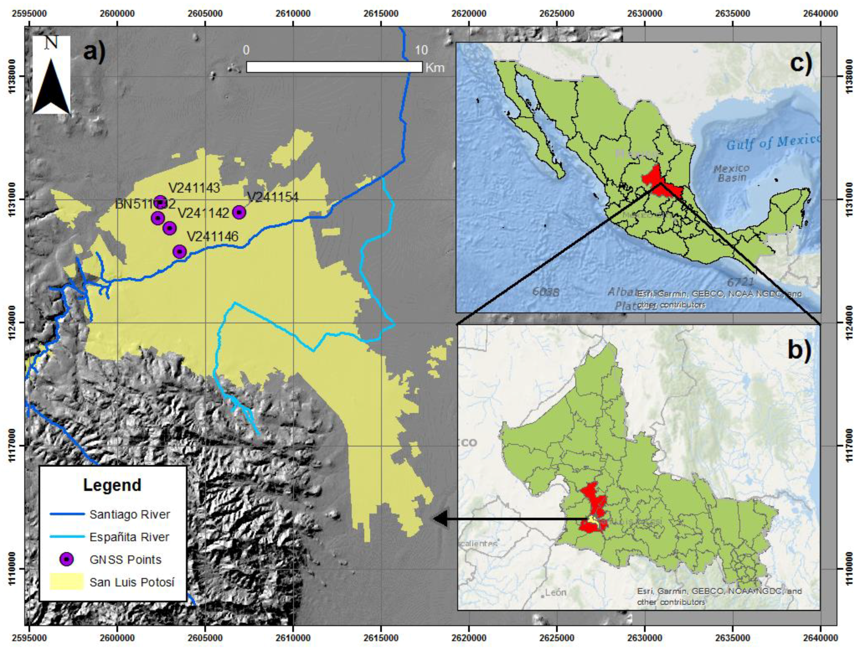
2.1. Description of San Luis Potosi Valley

The metropolitan area of the SLPV is located on a tectonic graben, delimited to the west by the Sierra de San Miguelito and to the east by the Sierra de Álvarez, occupying an area of 1980 km² at an altitude of 1850 m a.s.l. [46] (Figure 1a). Geographically, the valley is placed southwest of the state of San Luis Potosi (Figure 1b), in north-central Mexico, approximately 400 km from Mexico City (Figure 1c) [30,47,48]. The climate is semi-arid with an average annual rainfall, temperature, and potential evaporation of 365 mm, 17.6 °C, and 2000 mm, respectively [48].

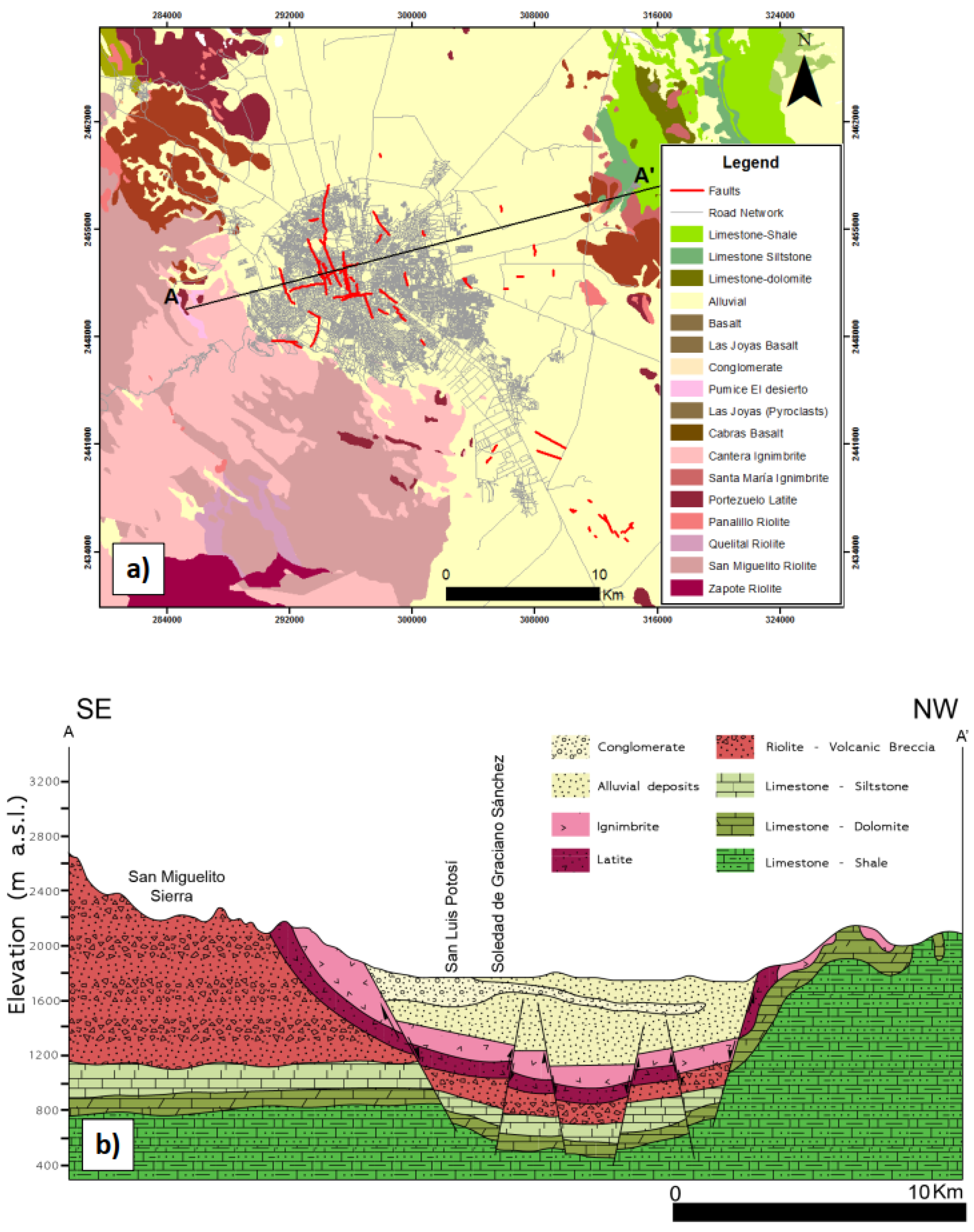
2.2. Geological Settings

The study area has a tectonic origin and was formed from a tectonic basin limited by a staggered N-S faults system forming a graben. This graben was filled over the years by pyroclastic material and alluvial and lacustrine sediments. The oldest rocks belong to the Cretaceous with ages of up to 125 million years. They are sedimentary rocks with a marine origin that outcrop towards the east in the Sierra de Álvarez and are mainly formed by limestone interbedded with shales and dolomites [49,50,51]. Cretaceous rocks are overlaid by Cenozoic volcanic rocks from the Sierra Madre Occidental province; the rocks that make up this volcanic belt include rhyolites, ignimbrites, and extensive pyroclastic flows. This extensional volcanic sequence has the Cenozoic tectonic signature, forming a series of horst and graben delimited by normal faults with a dominant and regional inclination between 15–20° NE. Quaternary conglomerates, volcanic ash, and alluvial deposits, (gravels, sands, silts, and clays, filling the graben) (Figure 2a) complete the stratigraphic sequence [52].

The profile A-A (Figure 2b) with SW-NE direction, shows information about the subsoil. The alluvial Quaternary deposits reach up to 600 m in the center of the valley where the graben reaches its maximum depth. Normal faults, typical of a horst and graben complex, are also identified. The volcanic sequence overlays the basement of the basin, composed of the Cretaceous sedimentary rocks.

2.3. Groundwater Pumping and Piezometric Evolution

The San Luis aquifer system is composed of two aquifers separated by a layer of thin, poorly, and permeable clay. The upper aquifer is composed of granular material from Quaternary deposits, with a maximum thickness of 250 m [53]. The deep aquifer is composed of Quaternary sediments, as well as strongly fractured volcanic rocks. These waters are approximately 6,300 years old, which indicates that the recharge dynamics are very slow [50,51]. Cretaceous sedimentary rocks are impermeable, so they represent the lower limit of the aquifer.

By 1960, 59% of the water for domestic use came from surface water and the rest was extracted from the aquifer, but today 84% of the water demand in the valley is covered by groundwater. The extraction of groundwater from the deep aquifer began in the 1940s. However, the historical data show that since 1972 the average drawdown rate is greater than 1 m/year and that between 1971 and 2005, the decrease in static levels was 95 m. Currently, the groundwater level is located at 170 m depth, and there are almost 200 authorized wells, which withdraw an approximate annual volume of 153.42 million m³, while the annual recharge volume corresponds to 78 million m³. Therefore, the aquifer system can be considered as overexploited, presenting an important deficit in the recovery of the San Luis Potosi groundwater levels [46,47,54,55].

3. Methods and Data Processing

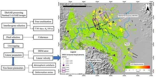
3.1. The Coherent Pixel Technique

The Coherent Pixels Technique (CPT) algorithm was developed at the Universitat Politècnica de Catalunya as an advanced DInSAR technique to extract the linear and non-linear movement from a set of differential interferograms and coherence images, as well as the DEM error and atmospheric artifacts [37,56]. A differential interferogram is a regular interferogram whose topographic component has been removed. This component is calculated using the orbital information and the external DEM. The actual interferogram phase of a single pixel contains not only the deformation between the times of acquisition of the two SAR images, but other terms that can hide the desired information. The aim of this processing is to isolate the deformation term from the rest in the set of interferograms. The following expression shows all the interferometric phase terms [45]:

$$\varphi \left(T,B_n\right)=\frac{4\pi }{\mathsf{\lambda }}.\left(v.T+\beta \right)+\frac{4\pi }{\mathsf{\lambda }}\frac{B_n}{r_{0}sin\theta }.\epsilon +n_{atm}+n$$

(1)

where $\varphi$ is the interferometric phase in a pixel, $\mathsf{\lambda }$ is the wavelength, $T y B_n\left(T\right)$ are the temporal and perpendicular baselines, $v$ is the deformation lineal velocity, $\beta$ is the non-linear deformation, $r_0$ is the sensor target distance, $\theta$ is the local incidence angle, $\epsilon$ is the DEM error, $n_{atm}$ corresponds to the atmospheric phase artifacts, and $n$ is the noise associated with the different decorrelation sources [45].

The CPT approach can be divided into four main blocks. The first one consists in the optimization of the selection of the interferograms considering their temporal and spatial baselines to maximize the detection of pixels, optimize the extraction of the deformation and DEM error, and reduce the amount of data to process. The second step is the pixel selection, during which only those pixels that have an enough phase quality are selected. The conventional selection approaches are based on evaluating the mean coherence along the set of interferograms, which work with multi-looked interferograms at a lower resolution, or the pixels’ amplitude stability of the SLC images, which allows work at full resolution. Due to the characteristics of the scene, the former approach has been used in this study. The third step is the estimation of the deformation linear term. To this aim, the algorithm considers the linear velocity of deformation and the DEM error through an adjustment of a linear model to the data. The last step is the estimation of the non-linear term of deformation. Once the linear term of the deformation and DEM error have been calculated and their contribution removed from the interferograms, CPT takes advantage of the different behavior of the atmospheric artifacts and non-linear term of deformation to separate their contributions to the phase. In this step, combinations of temporal and spatial filters are applied to extract the atmospheric phase screens for each image and the non-linear term of deformation [45,56].

3.2. Data Processing

In this paper, 112 Sentinel-1 images were processed, which were acquired from 25 October 2014 to 28 November 2019, with descending orbits in Interferometric Wide Swath (IWS) mode. The Single Look Complex (SLC) images correspond to dual-polarization (VV+VH) data with a swath extent of 250 km and a spatial resolution of 22 m in azimuth and 2.7 to 3.5 m in slant-range. Only the VV channel was used in the processing.

The first stage of CPT processing is the generation of the differential interferograms. The set of SLC images is selected, as well as the DEM that will be used to extract the topography and the region of interest (ROI) that is defined with a polygon. Once the images have been co-registered to a single master, chosen to minimize the maximum spatial and temporal baselines of the set, the interferograms are selected, among all possible, if they have spatial baselines smaller than 100 m and temporal baselines smaller than 365 days. With this criterion, 2118 interferograms were generated and a multilooking of 3 in azimuth by 15 in range was applied. The three arc-second Shuttle Radar Topography Mission (SRTM) DEM of the area, provided by the National Aeronautics and Space Administration (NASA), was used to remove the topographic phase component and, at the end of the process, geocode the results. With the differential interferograms, their associated coherence maps are generated as well. The coherence is a good estimator of the phase quality based on multi-looked interferograms and will be used on the pixel selection step. Coherence ranges from 0, fully decorrelated or pure noise phase, to 1, coherent or noiseless phase.

In the second stage, the differential interferograms are processed to obtain the deformation time-series, which included the linear and non-linear terms, and the DEM error, which are used to improve the geocoding of the results. Not all pixels of the scene are suitable for its processing due to different decorrelation phenomena, like the temporal decorrelation. Among the different pixel selection criteria, the coherence-based one was used. Therefore, all pixels with a mean coherence value below 0.6 and a phase standard deviation of 10° were discarded. Figure 3 shows the coherence map generated by CPT for the San Luis Potosi Valley, in which the brightest areas are the most coherent and correspond to the urbanized elements, such as buildings and houses, because these objects show very little change over time; on the other hand, the darkest areas correspond to agricultural areas, they have the lowest coherence values because the vegetation does not remain constant over time and induces temporal decorrelation on the interferometric phase. Consequently, it is expected that most of the pixels selected are within the urban area.

During the linear processing, CPT calculates the relative linear velocity change and DEM error among neighboring pixels. The absolute values for each pixel are obtained after an integration of these increments. As in any integration process, the solution presents an unknown offset that must be adjusted. This is done with a set of “seeds” that are pixels whose deformation rate and DEM error are known. They are usually selected in stable areas of the scene to minimize errors.

In this research, five seeds were chosen (Figure 4), one within the metropolitan area and four in the mountainous area, being careful that there is no evidence of active geomorphological processes in these points.

Once the linear velocity and DEM error terms have been calculated, the last stage is the non-linear processing. Once the non-linear term of deformation has been estimated, the final results are geocoded to the preferred datum.

3.3. GNSS Data Processing

In 2014, Instituto Nacional de Estadística y Geografía (INEGI), in collaboration with the Engineering Faculty of the Autonomus University of San Luis Potosi, led a campaign to measure GPS benchmarks with GNSS receivers in land subsidence areas, where structural damage had been detected in the SLPV. From INEGI information, positioning data for some vertices were re-measured in April 2020 using the static model with Trimble R8s GNSS receivers (Figure 1a). Static positioning is where a receiver is set up on top of a tripod at point of interest, taking information from a minimum of four satellites and for up to one hour, with an adequate Position Dilution of Precision (PDOP); from this, it would potentially lead to a better solution for the unknown ambiguity N, and better solutions of position X, Y, and Z [57]. In the 2020 field campaign, stationary receivers took observations from a minimum of 12 satellites, every 10 s for up to two hours, and PDOP values from 1.1 to 2.4, to achieve a more precise position.

The GNSS observation files were processed with the Trimble Business Center (TBC) 5.10 software, satellite orbit and clock parameters were provided by International GNSS service (IGS). Being a rigorous process, it was necessary to correct the tectonic plate velocity. This extrapolation was made from the ITRF08PR software developed by INEGI and applied to the GM10 (Mexico 2010) geoidal model.

4. CPT Results and Analysis

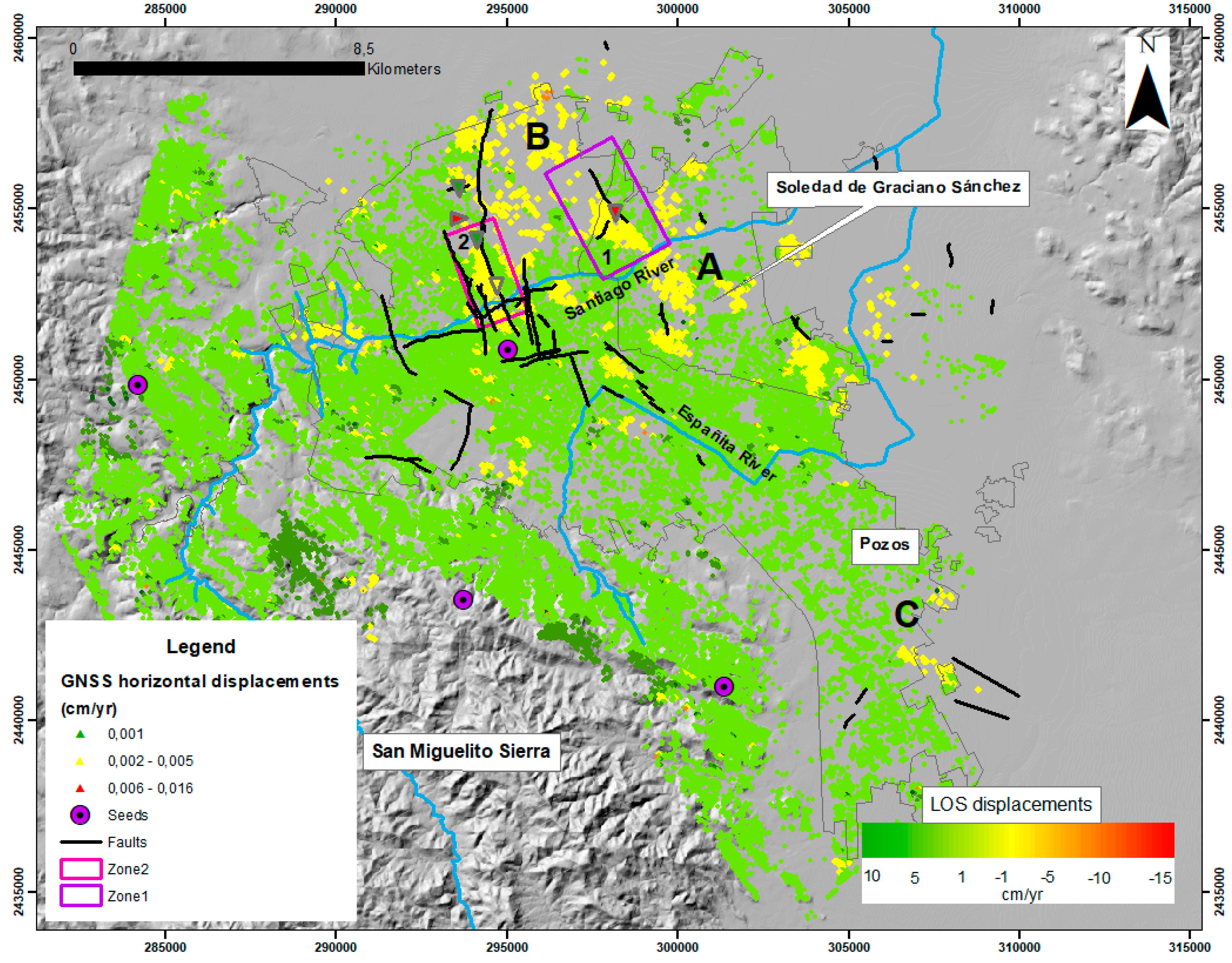
4.1. Deformation Rate Map

Figure 4 shows the result of the deformation rate along the line of sight (LOS) for the InSAR processing of Sentinel-1 dataset from 25 October 2015 to 28 November 2019.

The total number of pixels calculated from the Sentinel-1 dataset by the CPT technique reached 33,486. The SLPV shows a high deformation rate with an average velocity of up to -15 cm/year in the LOS direction from 2014 to 2019 located in the north center of the metropolitan zone. The stability range was defined by the standard deviation of the whole coherent pixel dataset. As a result, all the values between -1 and 1 cm/year are considered stable, these pixels in green color are located mainly at the south and the west of the study area. The positive values of the rate map indicate that the surface is uplifting. Most of these values are located in the San Miguelito Sierra mountains; the movement may be related to the tectonic and isostasy of the orogenic process. On the contrary, negative values indicate subsidence that is mainly located in the flood plain area. The deformation areas to the center-east in the municipality of Soledad de Graciano Sánchez (A in Figure 4) mostly have a value between −1.5 to −3.5 cm/year; whereas, in San Luis Potosi this value is between −1.8 and −4.2 cm/year in the north center of the valley (B in Figure 4). But there is also an isolated deformation area situated in “Pozos” (C in Figure 4) to the southeast of the SLPV in the industrial park. This site exhibits average displacement rates between −1.3 and −2.0 cm/year.

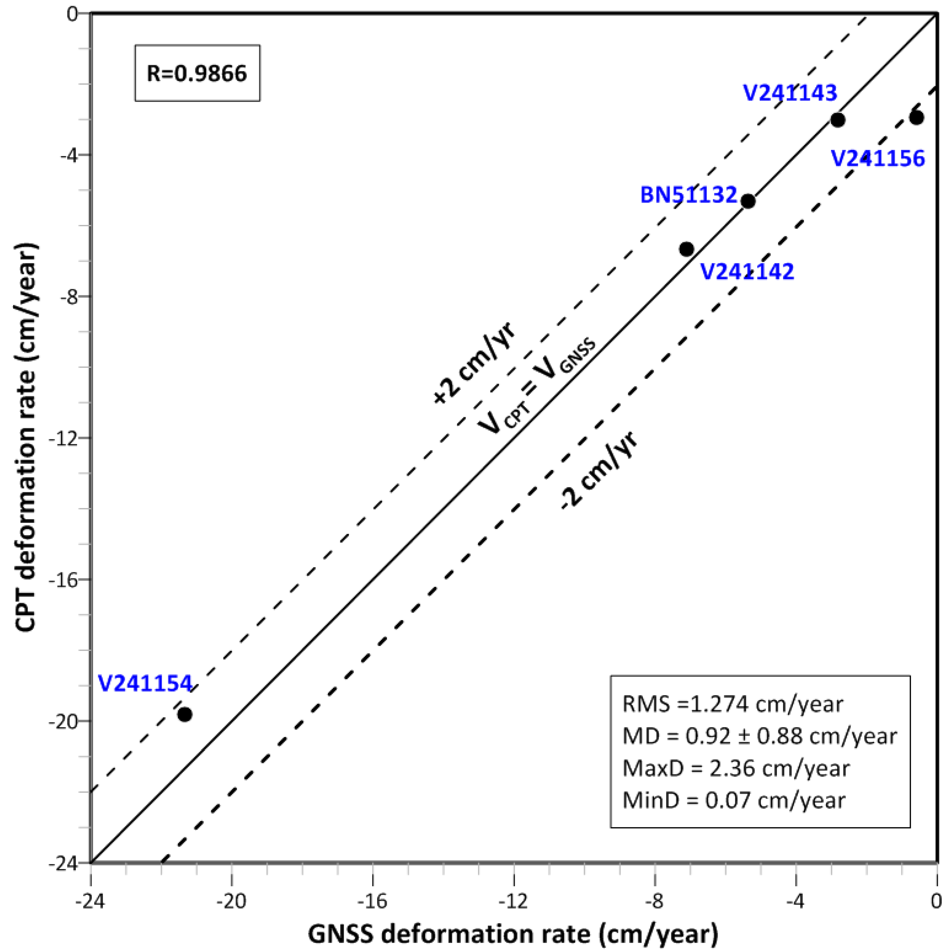
4.2. Validation of Results

To validate the PSI results, a comparison with in situ instrumental data acquired by a static post-process GNSS positioning method was conducted for five available points, providing horizontal and vertical displacements; the location of these points is shown in Figure 1, and they are equipped with Trimble R8s GNSS receivers and dual-frequency observations.

GNSS measurements provide vertical and horizontal displacement values. GNSS vertical values vary between −3.06 and −0.12 cm/year in the five stations for the period of 2013–2020. On the contrary, horizontal displacements for the period 2013–2020 are almost negligible, exhibiting total displacement rates ranging from 0.001 to 0.016 cm/yr.

To compare GNSS and Sentinel-1 displacements, GNSS vertical displacement values were multiplied by the cosine of the satellite look angle, in this case, Ɵ = 34.24º. Thus, it was necessary to project the GNSS settlements along the LOS for a direct comparison. To calculate the differential deformation along the LOS for each GNSS station, a 150 m diameter circular buffer area was defined around the five GNSS points. The differences between both techniques are calculated comparing the average deformation rate values for the period of 2014 to 2019 from all pixels contained within the buffer area with the subsidence rate of the considered GNSS.

Figure 5 shows the scatter plot of GNSS and CPT solutions for the five available GNSS vertices. This figure shows that the maximum discrepancy (MaxD) is 2.6 cm/year, and the minimum discrepancy (MinD) is 0.07 cm/year. The mean absolute discrepancies (MD) are 0.92 cm/year, and the root means square (RMS) is 1.27 cm/year. The data correlation between GNSS and PS-InSAR measurement is 0.986. This validation results suggest that InSAR derived results agree well with the results obtained by GNSS data.

5. Discussion

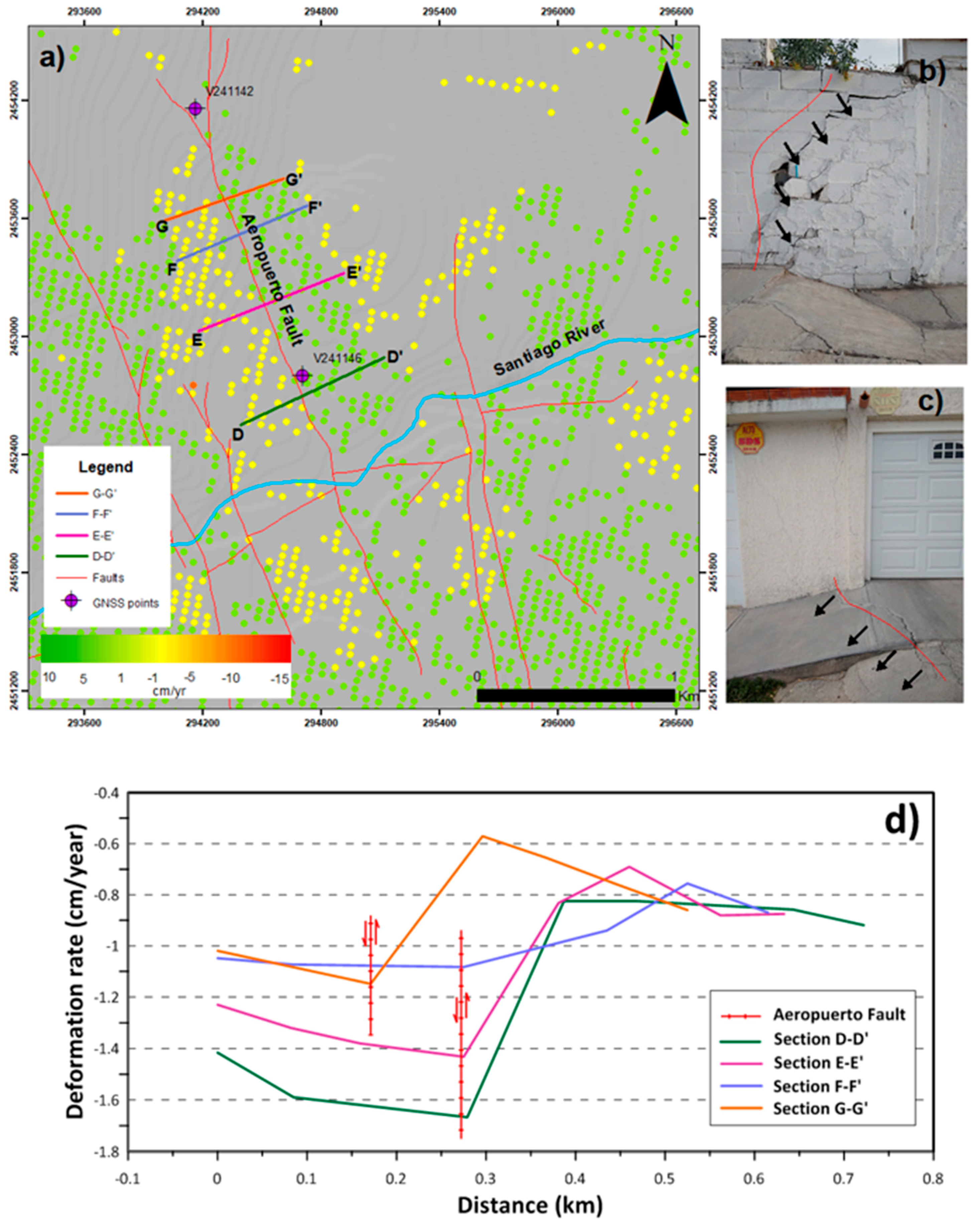
5.1. Relationship between Faults and Land Subsidence

Most of the active faults of the SLPV are normal with a north-south strike and are mainly distributed throughout the center-north areas of the city, affecting several buildings in the historic center. The main roads located on the Santiago river, the main affluent of the SLPV watershed, are also damaged by the faults’ activity. The principal faults on the SLPV present stress and subsidence structures by extension. In SLPV, it could be suggested that surficial fault movement is caused by water level decay and the associated land subsidence. The movements often develop on ground surface following the trace of preexisting blind faults affecting the bedrock. The sediment thickness accumulated over the hanging wall of the fault is much higher than the one accumulated on the footwall, creating a differential subsidence that causes tensional stresses [58], and that usually concentrates where the thickness of the soft soil changes drastically due to the bedrock heterogeneity. Frequently, this differential compaction of sediments produces tensile failures in subsurface materials that pull apart the ground [58,59] creating earth fissures; this type of failure is associated with groundwater withdrawal, and is clearly identified after extreme rains that produce flooding in some areas north to the SLPV. During these large rain events, hairline cracks caused by land subsidence intercept surface runoff, causing soil erosion and opening the earth fissure up to create a fissure gullies [59]. Municipal Civil Protection has reported earth fissures of 1 km in length and 6 m in width (Figure 6) in peripheral flat zones, potentially floodable, where the surface runoff or flow of water that descends from the mountains accumulates during the rainy season.

PSI deformation map shows spatial correlation with major faults, suggesting that these faults are still active and indicating the existence of a spatial control of land subsidence. The SLPV tectonic controlled by horst-graben structure has generated a basin with variable thickness and composition of sediments. Groundwater withdrawal has resulted in subsidence induced by faulting, which follows the pattern of structural faults buried by sediments. The obtained PS-InSAR results clearly delineate some fault traces. For example, the results show a change in the deformation velocity of the PSs along the San José del Terremoto fault. Green pixels display the stable velocity zone while yellow pixels display the area of greatest deformation. The time series constructed with the data derived from the PS-InSAR analysis shows accumulated deformations of 18 cm (Figure 7b). The settlements associated with the fault activity are evidenced in the structural damage produced on the road in the Villas de San Lorenzo neighborhood (Figure 7c). The GNSS point V241154 was located in the zone of greatest deformation of the fault, and GNSS measurements also indicated deformations of almost −20 cm. Sections B-B’ and C-C’ show the PS-InSAR deformation rates across the above mentioned fault with maximum velocities of −4 cm/year, in agreement with the structural dynamics of the area.

The trace of the Aeropuerto fault was also detected by PS-InSAR measurements (Figure 8a). This fault triggered tension cracks that are parallel and staggered in several areas of the SLPV metropolitan area. The change in the deformation velocities is very clear at both sides of the fault. The trace extends to the Santiago River, where damage evidence can be also seen, causing staggering on the road. Figure 8b,c show structural damage to the walls, the pavement, and the sidewalks. Land subsidence in this area has even led to the demolition of the affected buildings. Sections D-D’, E-E’, F-F’, and G-G’ across the fault show subsidence with deformation rates of up to −1.5 cm/year.

For both analyses, the fault trace is close to the subsidence boundary, suggesting a relationship between land subsidence and faults. In these cases, ground discontinuities and spatial sinking pattern are aligned along the fault direction; this is related to bedrock with buried tectonic faults, in this configuration, developed by a conceptual model know as Subsidence-Creep-Fault Processes [3,26], where land subsidence occurs due to the contrast in sediments thickness of both sides of the fault trace. So, InSAR is an efficient method to map these trace faults, and then could be useful for complete the geological map as well as to monitor these areas at risk, to avoid structure damages and improve the urban planning.

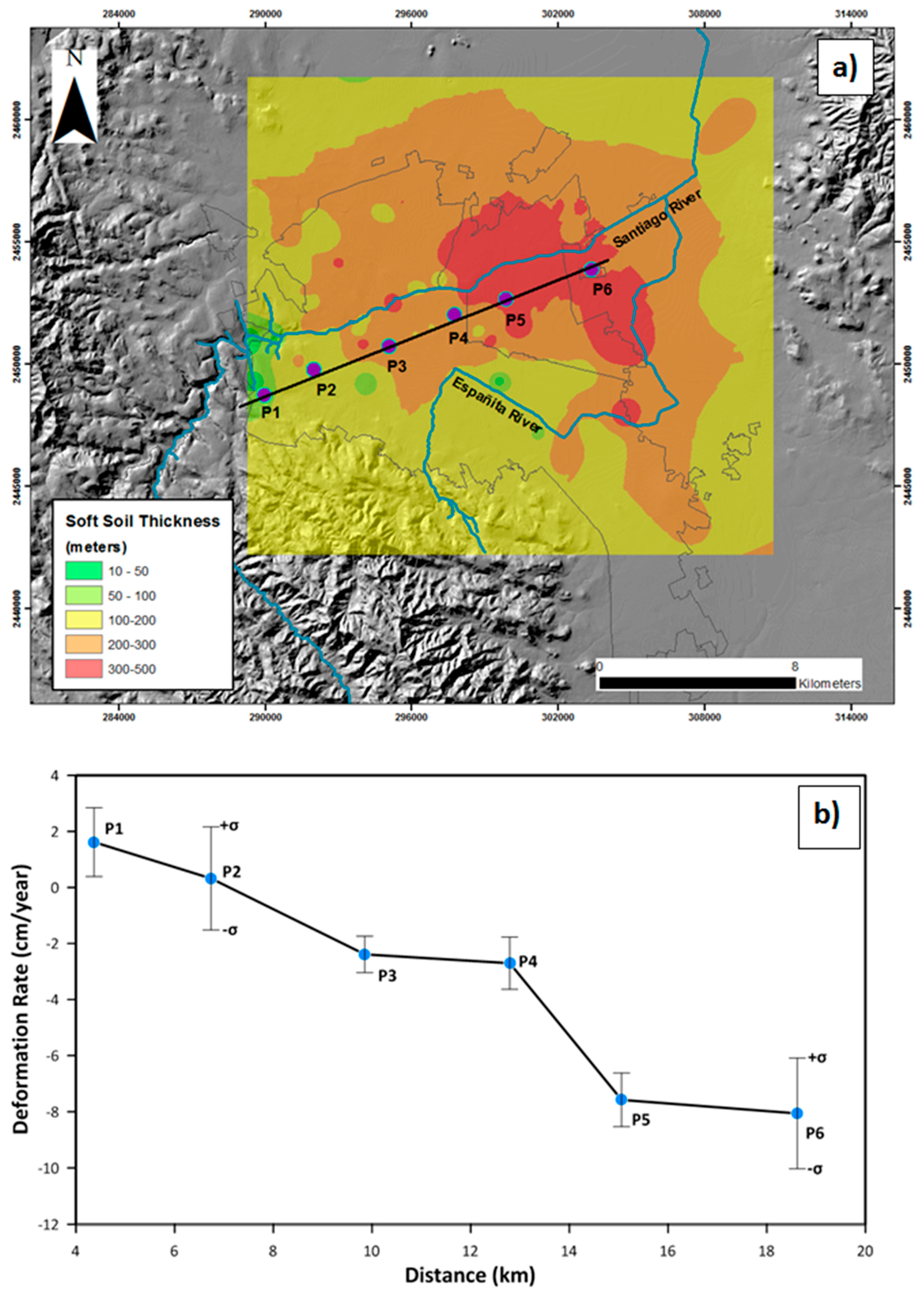
5.2. Relationship between Soft Soil Thickness and Land Subsidence

The mechanical response of the aquifer system to the increase in the effective stress and the distribution and thickness of unconsolidated soils play a key role in the magnitude of the developed settlements. As previously described, the SLPV aquifer system develops over a thick layer of alluvial sediments of different granulometry with accumulated thickness of up to 600 m. Therefore, in this section, the distribution of soft soil thickness derived from boreholes located throughout the study area is compared to the land subsidence measured by PS-InSAR (Figure 9a).

To explain the dependence of settlements on the sediment thickness and the mechanical response of the soil (i.e., its deformability), the following equation is utilized [60]:

$$\Delta \mathrm{D}=\Delta \mathrm{h}\times \mathrm{D}\times {\mathrm{S}}_{\mathrm{sk}}=\Delta \mathrm{h}\times {\mathrm{S}}_{\mathrm{k}}$$

(2)

where ∆D is the settlement of a deformable layer D meters thick, ∆h is the decrease in the static groundwater level (i.e., the groundwater level under non-pumping conditions) in meters, ${\mathrm{S}}_{\mathrm{s}\mathrm{k}}$ is the specific skeletal storage coefficient (m⁻¹) that represents the deformability of the aquifer system (dimensionless), and ${\mathrm{S}}_{\mathrm{k}}$ is the skeletal storage coefficient [18].

According to Equation (2), if there is a decrease in the groundwater static level there will be an increase in stress (i.e., Δh will increase) causing permanent settlements in normally consolidated soils. These settlements will be higher in those areas with higher accumulated soft soil thickness (i.e., with higher D values). Complementarily, the magnitude of the deformation depends on how deformable a lithological layer is (i.e., depends on the storage coefficient, S_k).

Figure 9a shows the soft soil thickness distribution map. As can be seen, the soft soil thickness is greater in the center of the valley, where the graben is deeper, and the accumulated sediments reach their maximum thickness. The east and west boundaries of the basin are limited by mountains, which are composed of volcanic and sedimentary rocks. These rocks are more competent and less deformable than the poorly consolidated sediments that filled the basin during the Quaternary period. When comparing the most deformable soils with the subsidence zones, it was found that they coincide. For this purpose, a section was constructed through the point P1 to P6 (Figure 9b). The deformation rate values were generated from the InSAR analysis and calculated through six buffer analyses with 300 m radius.

The deformations obtained with the PS-InSAR data analysis coincide with the fact that with a greater soft soil thickness the value of subsidence increases. For example, in Figure 9b, the point P1 located in the yellow zone that is closer to the Sierra de San Miguelito (stable zone), has less soft soil thickness, and then its deformation values are very close to zero. Meanwhile points P5 and P6, that are closer to the central zone of the SLPV where the basin is deeper, have higher sediment thicknesses. These points have subsidence values that reach up to −8 cm of accumulated deformation (2014–2019). Consequently, the correlation between soft soil thickness and land subsidence in the San Luis Potosi Valley is confirmed.

5.3. Relationship between Piezometric Level Evolution and Land Subsidence

A total of 24 wells distributed in the San Luis Potosi Valley were used in this analysis. Figure 10 shows the prediction map of the piezometric level changes (i.e., Δh in Equation (2)) of the SLPV, obtained using ordinary kriging and a Gaussian semivariogram model for the period of 2007–2017.

The used dataset shows a concentration of wells with piezometric records for the 2007–2017 period in the central-eastern area. As a consequence, the prediction error propagates towards the west southwest and east, where less information is available. From these results, it can be confirmed that the higher piezometric drawdown is located in the central-eastern zone (mainly the urban spot) and the recovery of the static level in these years occurs mainly towards the northeast and southeast of the study area. Additionally, it is worth noting that the zones with the greatest drawdowns in the piezometric levels match those areas in which the greatest thickness of deformable materials (i.e., Quaternary deposits of sand, silt, and clay, poorly or normally consolidated) and a greater population density exist. Consequently, the extraction of groundwater is the most important driving factor of land subsidence in this area because the variations in soil stress causing settlements are related to the piezometric levels variations according to Equation(2). Therefore, this analysis confirms the tight relationship of piezometric changes with the land subsidence as well as with the soft soil thickness.

Figure 11 shows a comparison between the time series and static level evolution. As can be seen, during the decade from 2007 to 2017, piezometric levels of the aquifer system have continuously declined up to 43 m in some wells. Wells CN-11-39 and CN-11-42 show drops of the piezometric level of 28 m and irrecoverable deformations of −5 cm; while wells CN-11-327 and CN-11-861 show drawdowns of 9 m and 15 m respectively, and associated irrecoverable subsidence values lower than −3 cm.

Water in confined aquifer-systems comes from the decrease of void space, which results in the compaction of the system, and the expansion of the water contained in the voids due to pore pressure decrease. Therefore, the aquifer-system coefficient of storage (S) is calculated from two terms related to the compressibility of the matrix (S_k) of the aquifer-system and the water compressibility (S_w) [61] according to the following equation:

$$S={\mathrm{S}}_{\mathrm{k}}+{\mathrm{S}}_{\mathrm{w}}$$

(3)

${\mathrm{S}}_{\mathrm{k}}$ can take two different values depending on the response of the soil to the stress induced by the groundwater head variations [61,62]: inelastic, ${\mathrm{S}}_{\mathrm{kv}}$, and elastic, S_ke. More specifically, when the effective stress is less than the previous maximum stressing level (i.e., the preconsolidation pressure defined as the maximum level of past stressing of the soil) the compaction or expansion of both aquitards and aquifers is mostly elastic, and ${\mathrm{S}}_{\mathrm{k}}={\mathrm{S}}_{\mathrm{ke}}$ is considered in Equation (3). However, if the effective stress exceeds the preconsolidation pressure, the aquitard can suffer permanent skeleton rearrangements resulting in high and not fully recoverable compaction that is calculated considering ${\mathrm{S}}_{\mathrm{k}}={\mathrm{S}}_{\mathrm{kv}}$. In this aquifer system, the current piezometric level decreases are the maximum ever registered in this area, and, therefore, we assume that we exceed the preconsolidation pressure and thus ${\mathrm{S}}_{\mathrm{k}}={\mathrm{S}}_{\mathrm{kv}}$. Furthermore, in compacting aquifers ${\mathrm{S}}_{\mathrm{k}}$ is much greater than ${\mathrm{S}}_{\mathrm{w}}$ [63] and then we can rewrite Equation (3) as:

$$S\approx {\mathrm{S}}_{\mathrm{kv}}$$

(4)

The storage coefficient of an aquifer-system for one-dimensional consolidation in inelastic conditions $\left({\mathrm{S}}_{\mathrm{kv}}\right)$, attributable to deformation of skeleton, can be expressed as [64,65] according to Equation (2):

$${\mathrm{S}}_{\mathrm{kv}}=\frac{\mathsf{\Delta }\mathrm{D}}{\mathsf{\Delta }\mathrm{h}}$$

(5)

where ∆D is the vertical compaction (in m), measured by means of PS-InSAR data, for a ∆h piezometric level change (in m) equivalent to a change in effective stress.

In this work, Equation (4) has been used to calculate the storativity of the San Luis Potosi deep aquifer from the static water level drawdowns and InSAR deformation measurements displayed in Figure 11. The ratios of the change in displacement to the change in water level for the continuous and permanent drawdown represent the inelastic storage coefficient (S_kv) [63,64,65,66,67], providing values varying from 1.3 × 10⁻³ to 4.8 × 10⁻³, and an average value of 3.4 × 10⁻³. As can be seen, these values are similar, indicating that even if the magnitude of land subsidence is different for each location, subsidence displacements associated with the drawdown were proportional to the water-level changes. For example, at CNA-11-52, the water level changed 8 m with a corresponding settlement of −33 mm, and at CNA-11-861 for a groundwater level drawdown of 3 m the accumulated settlement was 4 mm, and then the ratios of the change in displacement to the change in water level (i.e., S_kv) for the drawdowns are similar (i.e., 4.1 × 10⁻³ and 1.3 × 10⁻³ for CNA-11-52 and CNA-11-861 respectively). It is worth noting that the observed differences in the values of S_kv calculated for the different locations can be due to different soil layering and soil compressibility of the aquifer system.

These storage coefficient values have been compared with those published in other studies that were obtained from pumping tests under confined conditions providing values varying from 4 × 10⁻⁴ to 1 × 10⁻³ [53]. In spite of the apparent coincidence between in situ and InSAR-derived values, we have to take into account that in situ values of storage coefficient obtained from pumping tests are often representative only of the most permeable fraction of the aquifer system (i.e., the aquifer units), since hydraulic head lowering in adjacent aquifers only propagates into aquitards in long-term groundwater usage, while the hydraulic head drawdown equilibrates in aquifer units in the short-term pumping test [66,68]. Moreover, the tested thickness in previous pumping storage coefficients is usually lower than that estimated for the whole sediment thickness, and thus the values can also slightly differ.

Although the time series may show also an elastic behavior of the aquifer associated with the seasonal groundwater level variations, it is not possible to evaluate this behavior because, unfortunately, the water table time series was plotted only using the annual values of 2007 and 2017.

6. Conclusions

In this work, land subsidence in the SLPV was analyzed with CPT using 112 Sentinel-1 images, from 2014 to 2019. The results obtained from this technique revealed deformation areas to the center-east in the municipality of Soledad de Graciano Sánchez mostly have a value between −1.5 to −3.5 cm/year; in San Luis Potosi this value is between −1.8 and −4.2 cm/year in the north center of the valley, however, a maximum LOS deformation was estimated at up to −15 cm/year in the metropolitan area. CPT results were validated by five GNSS measurements with a correlation coefficient of 0.986, indicating that this advanced InSAR technique is effective to monitor and detect settlements.

In this paper, it is concluded that the groundwater extraction in the San Luis Potosi valley is related to the drawdown of the piezometric level of the aquifer system. The continuous decline increases the effective stress acting on unconsolidated Quaternary sediments, and therefore, the areas with higher accumulated thickness consolidate. The consolidation of the soil produces settlements on ground surface affecting urban infrastructures. The performed analysis confirms that the higher the thickness of accumulated Quaternary soils is, the higher the magnitude of these settlements is.

In the San Luis Potosi Valley, we have recognized high settlements related to the faults of the substratum generated by the tectonic configuration of the graben. This is a more localized phenomenon that develops sharply, causing severe damage to buildings and other constructions. Besides, general subsidence is associated with water extraction that generates slower subsidence, especially in the north and northeast of the SLPV. These areas correspond to greatest thickness of soft soils and the greatest piezometric decays. It is also suggested that SLPV has a structurally controlled subsidence, and this mechanism is governed by buried tectonic faults affecting the bedrock. The faults from horst-graben structure have generated a basin with a variable thickness and compositions of sediments. Finally, the groundwater withdrawal has resulted in subsidence induced by faulting, which follows the pattern of structural faults buried by sediments.

In summary, the results of this work evidence the inelastic and continuous land subsidence that is affecting the Quaternary aquifer system of SLPV due to overexploitation. The key role played by the soft soil thickness and the ground water depletion on the magnitude of land subsidence has been confirmed. Furthermore, a strong structural control of land subsidence patterns by faults affecting the bedrock has been also observed in SLPV. In the future, the integration of the knowledge derived from this work with numerical models will enable local and water management authorities to predict land subsidence for different future scenarios and to design the corresponding mitigation measurements.

References

1. Galloway, D.L.; Bawden, G.W.; Leake, S.A.; Honegger, D.G. Land Subsidence Hazards. In Landslide L. Subsid. Hazards to Pipelines; U.S. Geological Survey: Reston, VA, USA, 2018. [Google Scholar]
2. Modoni, G.; Darini, G.; Spacagna, R.; Saroli, M.; Russo, G.; Croce, P. Spatial analysis of land subsidence induced by groundwater withdrawal. Eng. Geol. 2013, 167, 59–71. [Google Scholar] [CrossRef]
3. Figueroa-Miranda, S.; Tuxpan-Vargas, J.; Ramos-Leal, J.A.; Hernández-Madrigal, V.M.; Villaseñor-Reyes, C.I. Land subsidence by groundwater over-exploitation from aquifers in tectonic valleys of Central Mexico: A review. Eng. Geol. 2018, 246, 91–106. [Google Scholar] [CrossRef]
4. Bolger, B.L.; Park, Y.-J.; Unger, A.J.; Sudicky, E.A. Simulating the pre-development hydrologic conditions in the San Joaquin Valley, California. J. Hydrol. 2011, 411, 322–330. [Google Scholar] [CrossRef]
5. Declercq, P.-Y.; Gerard, P.; Pirard, E.; Perissin, D.; Walstra, J.; Devleeschouwer, X. Subsidence related to groundwater pumping for breweries in Merchtem area (Belgium), highlighted by Persistent Scaterrer Interferometry. Int. J. Appl. Earth Obs. Geoinf. 2017, 63, 178–185. [Google Scholar] [CrossRef]
6. Castellazzi, P.; Arroyo-Domínguez, N.; Martel, R.; Calderhead, A.I.; Normand, J.C.L.; Gárfias, J.; Rivera, A. Land subsidence in major cities of Central Mexico: Interpreting InSAR-derived land subsidence mapping with hydrogeological data. Int. J. Appl. Earth Obs. Geoinf. 2016, 47, 102–111. [Google Scholar] [CrossRef]
7. Sowter, A.; Bin, M.; Amat, C.; Cigna, F.; Marsh, S.; Athab, A. Mexico City land subsidence in 2014–2015 with Sentinel-1 IW TOPS : Results using the Intermittent SBAS ( ISBAS ) technique. Int. J. Appl. Earth Obs. Geoinf. 2016, 52, 230–242. [Google Scholar] [CrossRef]
8. Osmano, B.; Dixon, T.H.; Wdowinski, S.; Cabral-cano, E.; Jiang, Y. Mexico City subsidence observed with persistent scatterer InSAR. Int. J. Appl. Earth Obs. Geoinf. 2011, 13, 1–12. [Google Scholar] [CrossRef]
9. Hu, L.; Dai, K.; Xing, C.; Li, Z.; Tomás, R.; Clark, B.; Shi, X.; Chen, M.; Zhang, R.; Qiu, Q.; et al. Land subsidence in Beijing and its relationship with geological faults revealed by Sentinel-1 InSAR observations. Int. J. Appl. Earth Obs. Geoinf. 2019, 82, 101886. [Google Scholar] [CrossRef]
10. Bian, H.-F.; Zhang, S.; Zhang, Q.; Zheng, N.-S. Monitoring large-area mining subsidence by GNSS based on IGS stations. Trans. Nonferrous Met. Soc. China 2014, 24, 514–519. [Google Scholar] [CrossRef]
11. Zhu, L.; Gong, H.; Li, X.; Wang, R.; Chen, B.; Dai, Z.; Teatini, P. Land subsidence due to groundwater withdrawal in the northern Beijing plain, China. Eng. Geol. 2015, 193, 243–255. [Google Scholar] [CrossRef]
12. Chen, B.; Gong, H.; Lei, K.; Li, J.; Zhou, C.; Gao, M.; Guan, H.; Lv, W. Land subsidence lagging quantification in the main exploration aquifer layers in Beijing plain. China. Int. J. Appl. Earth Obs. Geoinf. 2019, 75, 54–67. [Google Scholar] [CrossRef]
13. Shi, X.; Wu, J.; Ye, S.; Zhang, Y.; Xue, Y.; Li, Q.; Yu, J. Regional land subsidence simulation in Su-Xi-Chang area and Shanghai City, China. Eng. Geol. 2008, 100, 27–42. [Google Scholar] [CrossRef]
14. Zhang, Y.; Zhang, J.; Wu, H.; Lu, Z.; Guangtong, S. Monitoring of urban subsidence with SAR interferometric point target analysis: A case study in Suzhou, China. Int. J. Appl. Earth Obs. Geoinf. 2011, 13, 812–818. [Google Scholar] [CrossRef]
15. Hu, R.L.; Yue, Z.Q.; Wang, L.C.; Wang, S.J. Review on current status and challenging issues of land subsidence in China. Eng. Geol. 2004, 76, 65–77. [Google Scholar] [CrossRef]
16. Chen, C.; Pei, S.; Jimmy, J. Land subsidence caused by groundwater exploitation in Suzhou City, China. Hydrogeol. J. 2003, 11, 275–287. [Google Scholar] [CrossRef]
17. Sun, H.; Zhang, Q.; Zhao, C.; Yang, C.; Sun, Q.; Chen, W. Remote Sensing of Environment Monitoring land subsidence in the southern part of the lower Liaohe plain, China with a multi-track PS-InSAR technique. Remote Sens. Environ. 2017, 188, 73–84. [Google Scholar] [CrossRef] [Green Version]
18. Tomás, R.; Herrera, G.; Cooksley, G.; Mulas, J. Persistent Scatterer Interferometry subsidence data exploitation using spatial tools: The Vega Media of the Segura River Basin case study. J. Hydrol. 2011, 400, 411–428. [Google Scholar] [CrossRef]
19. Herrera, G.; Fernández, J.A.; Tomás, R.; Cooksley, G.; Mulas, J. Advanced interpretation of subsidence in Murcia (SE Spain) using A-DInSAR data–modelling and validation. Nat. Hazards Earth Syst. Sci. 2009, 9, 647–661. [Google Scholar] [CrossRef] [Green Version]
20. Foroughnia, F.; Nemati, S.; Maghsoudi, Y.; Perissin, D. An iterative PS-InSAR method for the analysis of large spatio-temporal baseline data stacks for land subsidence estimation. Int. J. Appl. Earth Obs. Geoinf. 2019, 74, 248–258. [Google Scholar] [CrossRef]
21. Mahmoudpour, M.; Khamehchiyan, M.; Nikudel, M.R.; Ghassemi, M.R. Characterization of regional land subsidence induced by groundwater withdrawals in Tehran, Iran. Geopersia 2013, 3, 49–62. [Google Scholar]
22. Poluzzi, L.; Barbarella, M.; Tavasci, L.; Gandolfi, S.; Cenni, N. Monitoring of the Garisenda Tower through GNSS using advanced approaches toward the frame of reference stations. J. Cult. Herit. 2019, 38, 231–241. [Google Scholar] [CrossRef]
23. Castellazzi, P.; Garfias, J.; Martel, R.; Brouard, C.; Rivera, A. InSAR to support sustainable urbanization over compacting aquifers: The case of Toluca Valley, Mexico. Int. J. Appl. Earth Obs. Geoinf. 2017, 63, 33–44. [Google Scholar] [CrossRef]
24. Ochoa-González, G.; Carreón-Freyre, D.; Franceschini, A.; Cerca, M.; Teatini, P. Overexploitation of groundwater resources in the faulted basin of Querétaro, Mexico: A 3D deformation and stress analysis. Eng. Geol. 2018, 245, 192–206. [Google Scholar] [CrossRef]
25. Pacheco-Martínez, J.; Hernandez-Marín, M.; Burbey, T.J.; González-Cervantes, N.; Ortíz-Lozano, J. Ángel; Zermeño-De-Leon, M.E.; Solís-Pinto, A. Land subsidence and ground failure associated to groundwater exploitation in the Aguascalientes Valley, México. Eng. Geol. 2013, 164, 172–186. [Google Scholar] [CrossRef]
26. Avila-Olivera, J.A.; Garduño-Monroy, V.H. A GPR study of subsidence-creep-fault processes in Morelia, Michoacán, Mexico. Eng. Geol. 2008, 100, 69–81. [Google Scholar] [CrossRef]
27. Cigna, F.; Osmanoglu, B.; Cabral-Cano, E.; Dixon, T.; Ávila-Olivera, J.; Garduño-Monroy, V.; DeMets, C.; Mdowinski, S. Remote Sensing of Environment Monitoring land subsidence and its induced geological hazard with Synthetic Aperture Radar Interferometry: A case study in Morelia, Mexico. Remote Sens. Environ. 2012, 117, 146–161. [Google Scholar] [CrossRef]
28. Hernández-Marín, M.; Pachecomartinez, J.; Ramirez-Cortes, A.; Burbey, T.J.; Ortiz-Lozano, J.A.; Zermeño-De-Leon, M.E.; Guinzberg-Velmont, J.; Pinto-Aceves, G. Evaluation and analysis of surface deformation in west Chapala basin, central Mexico. Environ. Earth Sci. 2014, 72, 1491–1501. [Google Scholar] [CrossRef]
29. Teatini, P.; Carreón-Freyre, D.; Ochoa-González, G.; Ye, S.; Galloway, D.; Hernández-Marin, M. Ground ruptures attributed to groundwater overexploitation damaging Jocotepec city in Jalisco, Mexico: 2016 field excursion of IGCP-641. Episodes 2018, 41, 69–73. [Google Scholar] [CrossRef]
30. Julio-Miranda, P.; Órtiz-Rodríguez, A.; Palacio-Aponte, A.; López-Doncel, R.; Baroboza-Gudiño, R. Damage assessment associated with land subsidence metropolitan area, Mexico, elements for risk. Natural Hazards 2012, 64, 751–765. [Google Scholar] [CrossRef]
31. Tomás, R.; Romero, R.; Mulas, J.; Marturià, J.J.; Mallorqui, J.J.; Lopez-Sanchez, J.M.; Herrera, G.; Gutiérrez, F.; González, P.J.; Fernandez, J.M.G.; et al. Radar interferometry techniques for the study of ground subsidence phenomena: A review of practical issues through cases in Spain. Environ. Earth Sci. 2013, 71, 163–181. [Google Scholar] [CrossRef] [Green Version]
32. Khorrami, M.; Alizadeh, B.; Tousi, E.G.; Shakerian, M.; Maghsoudi, Y.; Rahgozar, P. How Groundwater Level Fluctuations and Geotechnical Properties Lead to Asymmetric Subsidence: A PSInSAR Analysis of Land Deformation over a Transit Corridor in the Los Angeles Metropolitan Area. Remote Sens. 2019, 11, 377. [Google Scholar] [CrossRef] [Green Version]
33. Zhou, L.; Guo, J.; Hu, J.; Li, J.; Xu, Y.; Pan, Y.; Shi, M. Wuhan Surface Subsidence Analysis in 2015–2016 Based on Sentinel-1A Data by SBAS-InSAR. Remote Sens. 2017, 9, 982. [Google Scholar] [CrossRef] [Green Version]
34. Dai, K.; Shi, X.; Gou, J.; Hu, L.; Chen, M.; Zhao, L.; Dong, X.; Li, Z. Diagnosing Subsidence Geohazard at Beijing Capital International Airport, from High-Resolution SAR Interferometry. Sustainability 2020, 12, 2269. [Google Scholar] [CrossRef] [Green Version]
35. Chen, M.; Tomás, R.; Li, Z.; Motagh, M.; Li, T.; Hu, L.; Gong, H.; Li, X.; Yu, J.; Gong, X. Imaging Land Subsidence Induced by Groundwater Extraction in Beijing (China) Using Satellite Radar Interferometry. Remote Sens. 2016, 8, 468. [Google Scholar] [CrossRef] [Green Version]
36. Aobpaet, A.; Cuenca, M.C.; Hooper, A.; Trisirisatayawong, I. Land subsidence evaluation usin InSAR time series analysis in Bankok metropolitan area. In Proceedings of the Fringe 2009 Workshop, Frascati, Italy, 30 November–4 December 2009. (ESA SP-677, March 2010). [Google Scholar]
37. Duque, S.; Mallorqui, J.J.; Blanco-Sánchez, P.; Monells, D. Application of the Coherent Pixels Technique (CPT) to urban monitoring. In Proceedings of the 2007 Urban Remote Sensing Joint Event, Paris, France, 11–13 April 2007; pp. 1–7. [Google Scholar] [CrossRef]
38. Rigo, A.; Béjar-Pizarro, M.; Martínez-Díaz, J.J. Monitoring of Guadalentín valley (southern Spain) through a fast SAR Interferometry method. J. Appl. Geophys. 2013, 91, 39–48. [Google Scholar] [CrossRef]
39. Raspini, F.; Loupasakis, C.; Rozos, D.; Adam, N.; Moretti, S. Ground subsidence phenomena in the Delta municipality region (Northern Greece): Geotechnical modeling and validation with Persistent Scatterer Interferometry. Int. J. Appl. Earth Obs. Geoinf. 2014, 28, 78–89. [Google Scholar] [CrossRef] [Green Version]
40. Amighpey, M.; Arabi, S. Remote Sensing Applications : Society and Environment Studying land subsidence in Yazd province, Iran, by integration of InSAR and levelling measurements. Remote Sens. Appl. Soc. Environ. 2016, 4, 1–8. [Google Scholar]
41. Van Der Horst, T.; Rutten, M.M.; Van De Giesen, N.; Hanssen, R.F. Monitoring land subsidence in Yangon, Myanmar using Sentinel-1 persistent scatterer interferometry and assessment of driving mechanisms. Remote Sens. Environ. 2018, 217, 101–110. [Google Scholar] [CrossRef] [Green Version]
42. Chaussard, E.; Wdowinski, S.; Cabral-Cano, E.; Amelung, F. Land subsidence in central Mexico detected by ALOS InSAR time-series. Remote Sens. Environ. 2014, 140, 94–106. [Google Scholar] [CrossRef]
43. Calderhead, A.I.; Therrien, R.; Rivera, A.; Martel, R.; Garfias, J. Advances in Water Resources Simulating pumping-induced regional land subsidence with the use of InSAR and field data in the Toluca Valley, Mexico. Adv. Water Resour. 2011, 34, 83–97. [Google Scholar] [CrossRef]
44. Sarychikhina, O.; Glowacka, E.; Suarez-Vidal, F.; Mellors, R.; Hernández, J.R. Aplicación de DInSAR a los estudios de subsidencia en el Valle de Mexicali. Boletín Soc. Geológica Mex. 2011, 63, 1–13. [Google Scholar] [CrossRef]
45. Blanco-Sánchez, P.; Mallorquí, J.; Duque, S.; Monells, D. The Coherent Pixels Technique (CPT): An Advanced DInSAR Technique for Nonlinear Deformation Monitoring. Pure Appl. Geophys. 2008, 165, 1167–1193. [Google Scholar] [CrossRef]
46. Flores-márquez, E.L.; Ledesma, I.K.; Arango-galván, C. Sustainable geohydrological model of San Luis Potosí aquifer, Mexico. Geofísica Int. 2011, 50, 425–438. [Google Scholar]
47. Martínez, S.; Escolero, O.; Kralisch, S. Water Management in San Luis Potosí Metropolitan Area, Mexico. Int. J. Water Resour. Dev. 2010, 26, 459–475. [Google Scholar] [CrossRef]
48. Lopez-alvarez, B.; Ramos-leal, J.A.; Leon, G.S.; Morán-ramirez, J.; Carranco-lozada, S.E.; Noyola-medrano, C. Subsidence Associated with Land Use Changes in Urban Aquifers with Intensive Extraction. Nat. Sci. 2013, 5, 291–295. [Google Scholar] [CrossRef] [Green Version]
49. Martínez-Hernández, J. Identificación de la Recarga Natural e Inducida en la Cuenca de San Luis Potosí. Ph.D. Thesis, Universidad Autónoma de San Luis Potosí, San Luis Potosí, Mexico, 2008. [Google Scholar]
50. Tristán-gonzález, M.; Aguillón-Robles, A.; Barboza-Gudiño, J.; Torres-Hernández, J.; Bellon, H.; López-Doncel, R.; Rodríguez-Ríos, R.; Labarthe-Hernández, G. Geocronología y distribución espacial del vulcanismo en el Campo Volcánico de San Luis Potosí. Boletín Soc. Geológica Mex. 2009, 61, 287–303. [Google Scholar] [CrossRef]
51. Martínez-Banda, L. Identificación de la Contaminación Difusa en el Acuífero Somero de la Ciudad de San Luis Potosí. Ph.D. Thesis, Univerisidad Autónoma de San Luis Potosí, San Luis Potosí, Mexico, 2005. [Google Scholar]
52. Aguillón-Robles, A. Cartografía Geológica de las Hojas Espíritu Santo, Pinos, El Obraje, Ojuelos, Edos. de San Luis Potosí, Jalisco, Guanajuato y Zacatecas. Ph.D. Thesis, Universidad Autónoma de San Luis Potosí, San Luis Potosí, Mexico, 1983. [Google Scholar]
53. Heiming, A. Numerical modeling with vertical flow component of the deep aquifer in the graben of San Luis Potosí, Mexico. Master’s Thesis, RWTH AAchen University, Aachen, Germany, 2016. [Google Scholar]
54. Noyola-Medrano, M.C.; Ramos-Leal, J.A.; Domínguez-Mariani, E.; Pineda-Martínez, L.F.; López-Loera, H.; Carbajal, N. Factores que dan origen al minado de acuíferos en ambientes áridos: Caso Valle de San Luis Potosí. Rev. Mex. Cienc. Geol. 2009, 26, 395–410. [Google Scholar]
55. CONAGUA. Actualización de la Disponibilidad Media Anual de Agua en el Acuífero San Luis Potosí (2411) Estado de San Luis Potosí; Diario oficial de la federación: San Luis Potosí, Mexico, 2015. [Google Scholar]
56. Domínguez, J.; Romero, R.; Carrasco, D.; Martínez, A.; Mallorquí, J.J. Advanced DInSAR based on Coherent Pixels: Development and results using CPT technique. In Proceedings of the Fringe 2005 Workshop, Frascati, Italy, 28 November–2 December 2005; Volume 610, pp. 1–6. [Google Scholar]
57. Awange, J.L. GNSS Enviromental Sensing: Revolutionizing Enviromental Monitoring; No. 9783540882558; Springer: Perth, Australia, 2018. [Google Scholar]
58. Galloway, D.; Jones, D.R.; Ingebritsen, S.E. Land Subsidence in the United States; U.S.Geolog.: Reston, VI, USA, 1999.
59. Conway, B.D. Land subsidence and earth fissures in south-central and southern Arizona, USA. Hydrogeol. J. 2015, 24, 649–655. [Google Scholar] [CrossRef]
60. Tomas, R.; Herrera, G.; Lopez-Sanchez, J.M.; Vicente, F.; Cuenca, A.; Mallorquí, J.J. Study of the land subsidence in Orihuela City (SE Spain) using PSI data: Distribution, evolution and correlation with conditioning and triggering factors. Eng. Geol. 2010, 115, 105–121. [Google Scholar] [CrossRef]
61. Béjar-Pizarro, M.; Ezquerro, P.; Herrera, G.; Tomás, R.; Guardiola-Albert, C.; Ruiz, J.; Fernández, J.; Marchamalo, M.; Martínez, R. Mapping groundwater level and aquifer storage variations from InSAR measurements in the Madrid aquifer, Central Spain. J. Hydrol. 2017, 547, 678–689. [Google Scholar] [CrossRef] [Green Version]
62. Galloway, D.L.; Burbey, T.J. Review: Regional land subsidence accompanying groundwater extraction. Hydrogeol. J. 2011, 19, 1459–1486. [Google Scholar] [CrossRef]
63. Galloway, D.L.; Hudnut, K.W.; Ingebritsen, S.E.; Phillips, S.P.; Peltzer, G.; Rogez, F.; Rosen, P.A. Detection of aquifer system compaction and land subsidence using interferometric synthetic aperture radar, Antelope Valley, Mojave Desert, California. Water Resour. Res. 1998, 34, 2573–2585. [Google Scholar] [CrossRef]
64. Riley, F.S. Analysis of borehole extensometer data from central California, in Land Subsidence, vol. 2, edited by L. K. Tison. Int. Assoc. Sci. Hydrol. 1969, 89, 423–431. [Google Scholar]
65. Tomás, R.; Lopez-Sanchez, J.M.; Delgado, J.; Mallorquí, J.J. Hydrological parameters of the vega media of the segura river aquifer (SE Spain) obtained by means of advanced DInSAR. In Proceedings of the 2006 IEEE International Symposium on Geoscience and Remote Sensing, Denver, CO, USA, 31 July–4 August 2006. [Google Scholar]
66. Galloway, D.L.; Hoffmann, J. The application of satellite differential SAR interferometry-derived ground displacements in hydrogeology. Hydrogeol. J. 2007, 15, 133–154. [Google Scholar] [CrossRef] [Green Version]
67. Tomás, R.; Herrera, G.; Delgado, J.; Lopez-Sanchez, J.M.; Mallorquí, J.J.; Mulas, J. A ground subsidence study based on DInSAR data: Calibration of soil parameters and subsidence prediction in Murcia City (Spain). Eng. Geol. 2010, 111, 19–30. [Google Scholar] [CrossRef]
68. Hoffmann, J.; Zebker, H.A.; Galloway, D.L.; Amelung, F. Seasonal subsidence and rebound in Las Vegas Valley, Nevada, observed by synthetic aperture radar interferometry. Water Resour. Res. 2001, 37, 1551–1566. [Google Scholar] [CrossRef]
Figure 1. (a) Delimitation of the metropolitan area of San Luis Potosi; (b) location in the state of San Luis Potosi and (c) within Mexico. Projected coordinate system: UTM, datum WGS84.
Remotesensing 12 03822 g001
Figure 2. Geological settings of San Luis Potosi Valley: (a) geological map of the study area. Projected coordinate system: UTM, datum WGS84; and (b) geological section A-A’ (adapted from INEGI, 2017).
Remotesensing 12 03822 g002
Figure 3. Average coherence map of the study area for Sentinel-1 (October 2014 to November 2019) in the radar coordinate system.
Remotesensing 12 03822 g003
Figure 4. Line of sight (LOS) deformation rates derived from Sentinel-1 for the metropolitan area of SLPV from 25 October 2014 to 28 November 2019. Black rectangles 1 denote the location of San Jose del terremoto fault, and rectangle 2 denotes a portion of the Aeropuerto fault area. Arrows represent GNSS-derived horizontal movements. Projected coordinate system: UTM, datum WGS84.
Remotesensing 12 03822 g004
Figure 5. Comparison between GNSS displacements projected along the LOS and PS-InSAR results. The location of the GNSS points is shown in Figure 2.
Remotesensing 12 03822 g005
Figure 6. (a,b) Earth fissures located north of the metropolitan area in the Antorcha neighborhood in 2018. Pictures Backgrounds Credits: Municipal Civil Protection.
Remotesensing 12 03822 g006
Figure 7. Deformation rate map derived by PS-InSAR covering (a) the San José del terremoto fault zone, colored lines represent sections across the trace fault. Projected coordinate system: UTM, datum WGS84. (b) Structural damage caused by surface subsidence in Villas de San Lorenzo neighborhood, (c) time series derived InSAR process for V241154 GNSS station, and (d) Land subsidence sections B-B’ and C-C’ along the fault.
Remotesensing 12 03822 g007
Figure 8. Deformation rate map derived by PS-InSAR covering (a) the Aeropuerto fault zone, colored lines represent sections across the trace fault. Projected coordinate system: UTM, datum WGS84. (b,c) Structural damage caused by surface subsidence in Industrial Aviación neighborhood, and (d) Land subsidence sections D-D’, E-E’, F-F’, and G-G’ along the Aeropuerto fault.
Remotesensing 12 03822 g008
Figure 9. Relationship between soft soil thickness and subsidence. (a) Soft soil thickness map of the SLPV. Projected coordinate system: UTM, datum WGS84. (b) Deformation rate values along the section P1–P6.
Remotesensing 12 03822 g009
Figure 10. Static level evolution of the San Luis Potosi Valley for the 2007–2017 period. Projected coordinate system: UTM, datum WGS84.
Remotesensing 12 03822 g010
Figure 11. Piezometric level evolution and deformation time series measured by the Coherent Pixels Technique (CPT) for different wells in SLPV. The location of the wells is shown in Figure 10. Blue points and dashed blue line represent the measured values and the general trend of static water level, respectively.
Remotesensing 12 03822 g011
Publisher’s Note: MDPI stays neutral with regard to jurisdictional claims in published maps and institutional affiliations.