Mapping Burned Areas of Mato Grosso State Brazilian Amazon Using Multisensor Datasets

Abstract

Quantifying forest fires remain a challenging task for the implementation of public policies aimed to mitigate climate change. In this paper, we propose a new method to provide an annual burned area map of Mato Grosso State located in the Brazilian Amazon region, taking advantage of the high spatial and temporal resolution sensors. The method consists of generating the vegetation, soil, and shade fraction images by applying the Linear Spectral Mixing Model (LSMM) to the Landsat-8 OLI (Operational Land Imager), PROBA-V (Project for On-Board Autonomy–Vegetation), and Suomi NPP-VIIRS (National Polar-Orbiting Partnership-Visible Infrared Imaging Radiometer Suite) datasets. The shade fraction images highlight the burned areas, in which values are represented by low reflectance of ground targets, and the mapping was performed using an unsupervised classifier. Burned areas were evaluated in terms of land use and land cover classes over the Amazon, Cerrado and Pantanal biomes in the Mato Grosso State. Our results showed that most of the burned areas occurred in non-forested areas (66.57%) and old deforestation (21.54%). However, burned areas over forestlands (11.03%), causing forest degradation, reached more than double compared with burned areas identified in consolidated croplands (5.32%). The results obtained were validated using the Sentinel-2 data and compared with active fire data and existing global burned areas products, such as the MODIS (Moderate Resolution Imaging Spectroradiometer product) MCD64A1 and MCD45A1, and Fire CCI (ESA Climate Change Initiative) products. Although there is a good visual agreement among the analyzed products, the areas estimated were quite different. Our results presented correlation of 51% with Sentinel-2 and agreement of r² = 0.31, r² = 0.29, and r² = 0.43 with MCD64A1, MCD45A1, and Fire CCI products, respectively. However, considering the active fire data, it was achieved the better performance between active fire presence and burn mapping (92%). The proposed method provided a general perspective about the patterns of fire in various biomes of Mato Grosso State, Brazil, that are important for the environmental studies, specially related to fire severity, regeneration, and greenhouse gas emissions.

1. Introduction

In Brazil, burning of vegetation biomass is a management practice used to create and to maintain cattle pasture and to expand agricultural frontier [1]. The burning practice is widely used in the production process in the Brazilian Amazon (rainforest) and Cerrado (savanna) biomes and is a factor that drives the agricultural expansion in these regions. Farmers burn their land to convert forests to cropland or pasture, to control the spread of weeds, pests, or diseases, and to stimulate pasture regrowth, as well [2,3,4,5,6].

Burns occur every year, and especially during the dry season, with most of the fires occurring towards the end of the dry season. During this time, risk of fire is highest due to factors, such as dry weather, the predominance of grass and other flammable materials, and increased exposure to ignition sources, such as flames, heated surfaces, sparks, lightning, and human action [7], facilitate the occurrence of the burning process [2,8,9,10]. Occasionally, non-anthropogenic factors, such as lightning, are also responsible for burning.

In the Legal Amazon, for example, it is estimated that at least 9% (1.99 million hectares) of the degraded primary forest areas were caused by fire during 2000–2013 time period [11]. In addition, prospects of forest degradation resulting from fires escaping from nearby agricultural areas into forests may be a growing risk in many regions in Brazil [12]. In this context, the intensity, duration, extent, and period of the year when fires occur will determine how a particular ecosystem will be resistant to this event and how it will recover to the previous state (resilient). In some cases, this phenomenon can be beneficial for vegetation, as is the case with pastures of the Brazilian savanna (Cerrado biome), where the low-intensity burning event accelerates the availability of nutrients for plants by mineralization [7]. However, successive burnings alter the rates of infiltration and evapotranspiration of water in the soil, increasing the soil’s susceptibility to wind and water erosion. Moreover, unlike the Brazilian Cerrado, the Amazon rainforest is not adapted to fire; therefore, vegetation in most cases is almost entirely consumed by burning, leading to a gradual increase of tree mortality [7,13].

Forest burning brings numerous environmental impacts, such as soil depletion and loss of biodiversity of flora and fauna [7], as well as causing significant damage to private properties and society as a whole [14]. In addition, trace gases and aerosols released by burning biomass cause changes in the energy balance of the atmosphere, leading to local, regional, and global climate changes [9,15]. Biomass burning in tropical regions contributes to ~32% of global CO emissions to the atmosphere. In this context, Cerrado is one of the most critical sources of trace gases due to the frequency and extent of burning [16,17], where the interaction of human activities mold temporal and spatial patterns of fires emissions [18].

Analysis of the timing and distribution of forest fires is a crucial tool for efficient fire management across regions experiencing various fire events. It provides information for fire prevention planning and is also critical for assessing economic losses and ecological effects, monitoring changes in land use and land cover, and developing atmospheric and climate impact models due to vegetation biomass burning [19].

Remote sensing represents a particularly useful tool for mapping and quantifying burned areas in large and difficult to reach areas. These data allow for active fire detection, which registers the instantaneous temperature of objects in combustion using spectral bands between 4 and 11 μm [20,21]; burned area estimation, which uses the spectral bands in the visible, near-infrared, and mid-infrared regions of the electromagnetic spectrum to detect changes in the spectral characteristics of land cover before and after the occurrence of fires [22,23]; fire patterns and severity [24,25]; and studies of vegetation regeneration and risk analysis [26,27]. Moreover, data derived from remote sensing are the most efficient source of information to understand the fire dynamics as they allow the observation of large areas of the surface at high temporal resolutions [28,29].

Several studies using burned areas (BA) detection algorithms have been conducted. Reference [30] used an algorithm based on Normalized Burned Ratio differencing (dNBR) to map the BA from MODIS (Moderate Resolution Imaging Spectroradiometer) data in three different ecosystems, such as boreal forest of Central Siberia, Mediterranean-type ecosystem of California, and sagebrush steppe of the Great Basin. The results showed that in each ecosystem, the BA estimates were within 15% compared to the high-resolution base, presenting a strong potential for regional and ecosystem-specific burned area mapping applications. Reference [31] developed a multitemporal two-phase burned area (BA) algorithm using Sentinel-2 MSI (MultiSpectral Instrument) reflectance images and active fires from MODIS sensors in the whole Sub-Saharan Africa. The algorithm used the spectral indices NBR2 (Normalized Burn Ratio 2), MIRBI (Mid Infrared Burn Index), and the NIR (near infrared) spectral region. The validation was based on a two-stage stratified random sampling of Landsat images and also compared to MCD64A1. The results showed an omission error of 26.5% and commission error of 19.3%, and, when compared to MCD64A1, the product presented an 80% larger area than NASA (National Aeronautics and Space Administration) BA product. The limitations found relies on the lower temporal resolution, impacting in the mapping due to cloud/cloud shadows.

In this context, some limitations increase errors in burned area products. Significant source of errors include the presence of clouds, which significantly reduces the ability to detect a fire hotspot due to the attenuation of the spectral radiance emitted by the flaming and smoldering phases in the biomass burning process [32], the lack of data on the moment of fire occurrence and, especially, the incompatibility of the temporal and spatial resolutions of some sensors, making these sensors unsuitable for the identification of burns. One way to reduce the uncertainty in the detection of burned surfaces is by using sensors data that have geometric, radiometric, and temporal resolutions appropriate to map the location and the discrimination of burned areas.

There are several global burned areas maps available, such as MODIS MCD45A1, MODIS MCD64A1, and Fire CCI (ESA Climate Change Initiative). However, in general, they present different results due to data characteristics, image dates, and applied methods for mapping [33,34]. These differences in the estimates occur because burning events are dynamics and affect different sizes on the ground, requiring sensors data with different spatial and temporal resolutions. For example, Landsat sensors [35,36] with a medium spatial resolution (30 m) are adequate to estimate the burned areas, but their limited temporal resolution (16 days) reduce their utility in the savanna and pastureland areas which regenerate rapidly following fires. In addition, product derived from Sentinel-2 imagery would greatly contribute to better understanding the impacts of small fires in global fire events. In contrast, the MODIS sensor with daily acquisition and moderate spatial resolution (250 m) provides useful information for the global mapping of burned areas but underestimates small fire scars [37,38]. Other sensors with similar high temporal resolution as MODIS for burned areas assessment include NPP-VIIRS (National Polar-Orbiting Partnership-Visible Infrared Imaging Radiometer Suite) and PROBA-V (Project for On-Board Autonomy–Vegetation) (at each 2 days) [39,40,41].

Combining information from different sensors can fill the gap between high temporal resolution and medium spatial resolution in an operational and accurate burned area product. However, this high volume of data requires approaches that highlight specific information to facilitate further classification tasks. An alternative approach to reduce the dimensionality of image data and enhance specific information for digital interpretation is the use of fraction images [42,43]. These images constitute synthetic bands with information on endmember proportions and they are generated by Linear Spectral Mixing Model (LSMM). For example, vegetation fraction images highlight the vegetation cover, especially cropland areas; soil fraction images highlight the contrast between forest and non-forested areas, and shade fraction images highlight water bodies and burned areas. In this manner, many efforts have been reported using LSMM to map burned areas, especially in the Brazilian Amazon [44,45,46].

The main objective of this work was to propose a new method to map burned areas using multisensor fraction images by taking advantage of the high temporal resolution of Suomi NPP-VIIRS and PROBA-V, and the medium spatial resolution of Landsat-8 OLI (Operational Land Imager) images for the year 2015. In order to evaluate the method, we use as reference the burned area map obtained using Sentinel-2 data, and compare our results with active fire data and the available monthly burned area products of MODIS MCD64A1, MODIS MCD45A1, and Fire CCI.

2. Materials and Methods

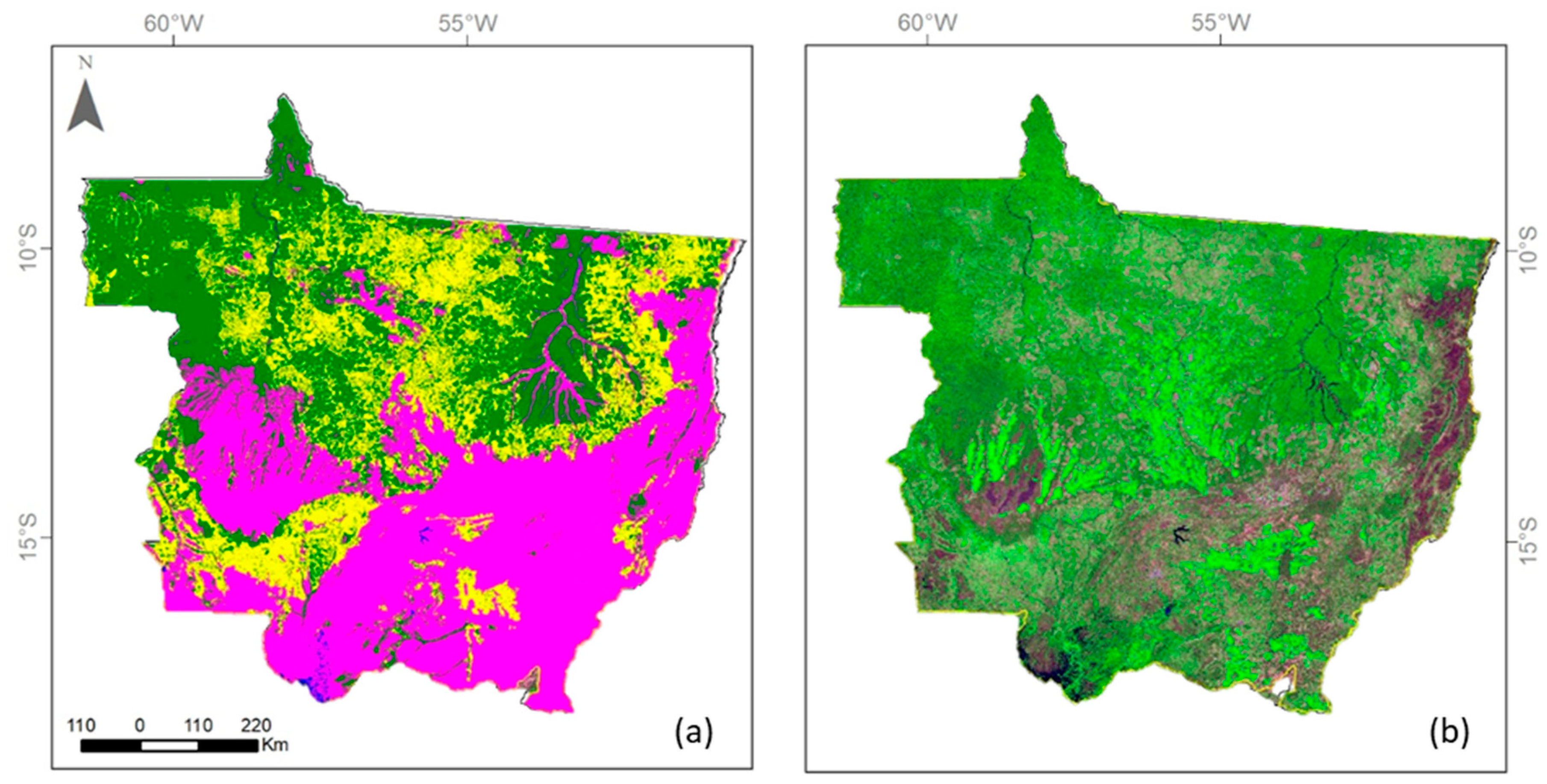
2.1. Study Area

The study area is Mato Grosso State (Figure 1), the third largest state in Brazil located in the central-west region and covering an area approximately 904,984 km². Mato Grosso State consists of three biomes: Amazon (54%), Cerrado (40%), and Pantanal (6%), according to the official Brazilian national classification system [47]. Mato Grosso State presents complex biodiversity, which, due to variable climate and terrain relief, resulted in different vegetation types. The Amazon biome consists of closed vegetation, high canopy, and a continuous layer of crowns; the Cerrado biome, a savanna formation, is characterized by tree species with tortuous trunks and typical openness canopy; and the Pantanal biome, a seasonal wetland, is composed by savannas and marshes [48].

Mato Grosso Sate stands out as a center of Brazilian agribusiness tied to illegal deforestation. The state falls partly within the ‘arc of deforestation’ in the southern part of the Brazilian Legal Amazon, an area with one of the highest annual deforestation rates. According to the Monitoring Deforestation of the Brazilian Amazon Forest by Satellite (PRODES) data [49,50], the Mato Grosso State has an accumulated deforestation (1988–2019) corresponding to 146,140 km² area, which represents approximately 16% of its territory. In terms of total degraded area, the state is the second in the ranking among the states of the Legal Amazon. Deforestation activities cause, among others, habitat fragmentation, which leaves the remaining forest more vulnerable to edge effects and fire [51,52].

Mato Grosso State is among the states that lead in the number of active fires detected [53]. For example, in the 1988–2020 period, 40,000 fires were detected in the state, accounting for approximately 27% of the total active fires observed in the Legal Amazon [53]. Most of the active fires occurred between June and November, a period with the least precipitation received. In the dry season, it is expected the increasing risk of the fire spreading and escaping, affecting nearby forest areas and causing forest degradation, that is an important source for the REDD+ program (Reduction of Emissions from Deforestation and Forest Degradation) since these areas remain as forest areas but with high ecosystem loss.

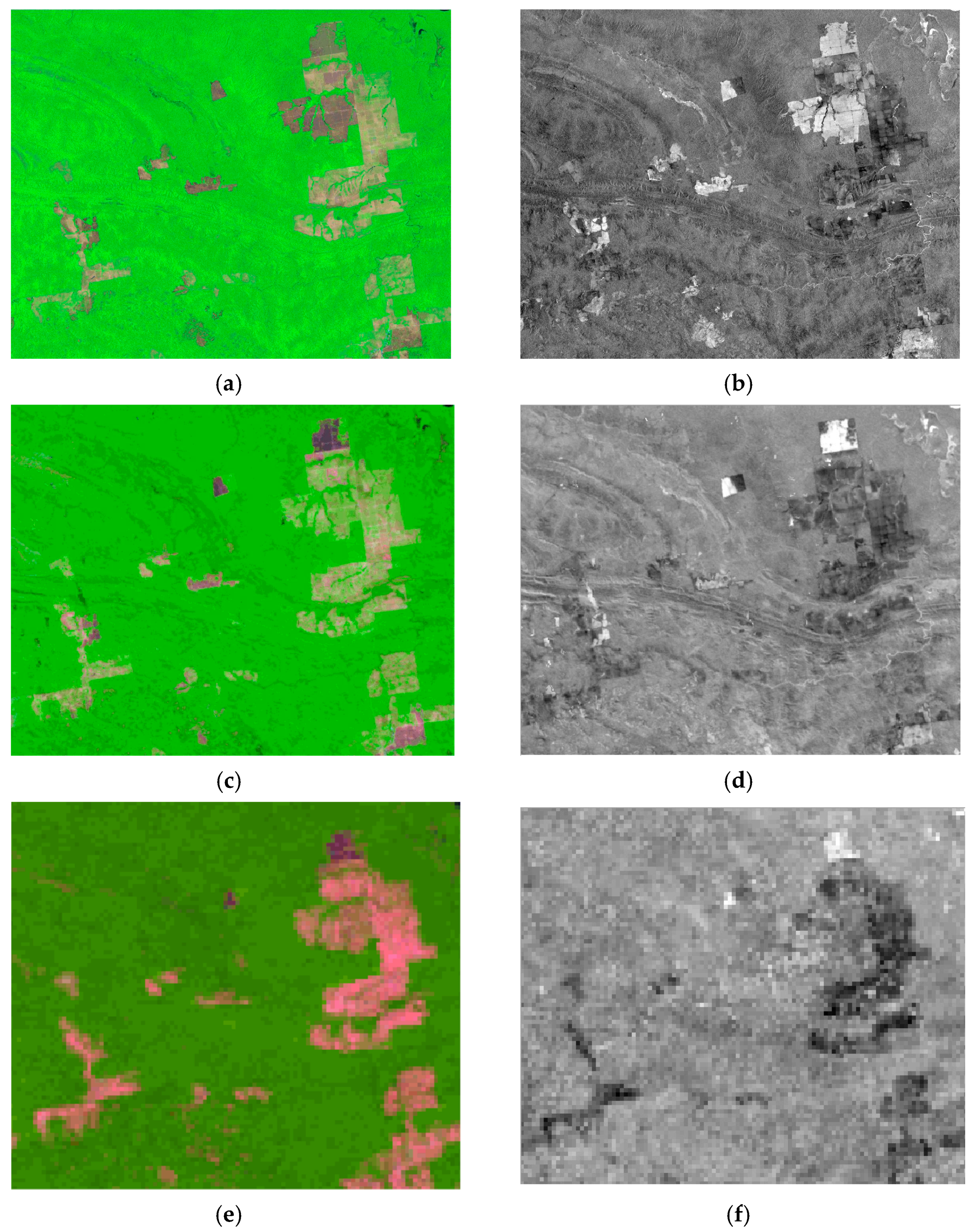
2.2. Remote Sensing Datasets

2.2.1. PROBA-V

We acquired data from PROBA-V, a mini-satellite designed as a continuity to the 15 years of the SPOT-VEGETATION (Satellite Pour l’Observation de la Terre–Vegetation) mission, and for the Sentinel-3 mission of the European Space Agency (ESA). To meet the user’s community, the spectral channels of the PROBA-V are similar to the SPOT VEGETATION instrument with four bands: blue (438–486 nm), red (615–696 nm), near-infrared (NIR) (772–914 nm), and medium infrared (MIR) (1564–1634 nm). The PROBA-V has a spatial resolution of 100 m at nadir and 300 m at the edge of scan.

In this study, we used 5-day Top-Of-Canopy PROBA-V image composite acquired at a spatial resolution of 100 m for the period between May and October 2015. The images were downloaded from the Vito Earth Observation portal (http://www.vito-eodata.be/PDF/portal/Application.html#Home), and all images had their clouds and respective shadows removed using the information from the Status Map layer in a program developed in the Interactive Data Language (IDL).

2.2.2. Suomi NPP-VIIRS

We downloaded 153 VIIRS daily reflectance (VNP09GA) images acquired between May and October 2015 from the U.S. Geological survey (USGS) at https://e4ftl01.cr.usgs.gov/VIIRS/VNP09GA.001/. The downloaded images consisted of three spectral bands, I1 (red, 600–680 nm), I2 (NIR, 846–885 nm), and I3 (MIR, 1580–1640 nm), and had a spatial resolution of 500 m. The 153 daily reflectance images were later composited into a cloud-free monthly VIIRS surface reflectance images using a script in Google Earth Engine and image quality flags 1 (QF1) layer.

2.2.3. Landsat-8 OLI

The Operational Land Imager (OLI) on Landsat-8 satellite has 11 spectral bands (panchromatic, 500–680 nm; multispectral, 430–450 nm; visible, 450–690 nm; NIR, 850–880 nm; MIR, 1570–2290 nm; cirrus, 1360–1380 nm; and thermal infrared, 10600–12510 nm). The sensor has a temporal resolution of 16 days and spatial resolution of 30 m except for the panchromatic band (15 m). The Landsat-8 OLI images were acquired during the dry season, from August to November, most acquired in October (41 images) and September (7 images), with August and November having only one image, due to the persistency of clouds (Appendix A). The images were downloaded from USGS archive: https://earthexplorer.usgs.gov/.

2.2.4. Sentinel-2 MSI

The Multispectral Instrument (MSI) on Sentinel-2A Level-1C dataset was used in this study as a reference to evaluate the burned areas classification by the proposed method. The Sentinel-2A MSI has 13 spectral bands from visible to SWIR (Short-wave Infrared) (B1, 432.2–453.2; B2, 459.4–525.4; B3, 541.8–577.8; B4, 649.1–680.1; B5, 696.6–711.6; B6, 733–748; B7772.8–792.8; B8, 779.8–885.8; B8A, 854.2–875.2; B9, 935.1–955.1; B10, 1358–1389; B11, 1568.2–1659.2; B12, 2114.9–2289.9). Each single satellite (2A and 2B) has a temporal resolution of 10 days and the combined constellation revisit is 5 days, with spatial resolution varying from 10 to 60 m. In this case, only bands with 10 m were used in this study. Due to the Sentinel-2A launch date (June 2015), only a segment of Mato Grosso State was available in 2015 in the period from August to November to compare the same period between the datasets used in this work. The images were downloaded from Joint Research Center website (https://jeodpp.jrc.ec.europa.eu/forobs/sentinel.py).

2.3. Global Burned Area Products

Burned area is considered as a non-permanent land cover change, and, in this manner, a variety of algorithms have been applied to detect and to map burned areas, leading to different results spatially and temporally [34]. In this work, the identified burned areas based on the proposed approach were spatially compared with three available global burned area products for an agreement analysis (

Table 1. Overview of burned area products selected for agreement analysis.

Producer	Product	Collection	Sensor	Spatial Resolution	Period
European Space Agency	Fire CCI	5.1	MODIS	250 m	Monthly
NASA MODIS Land Science Team	MCD45A1	5.1	MODIS	500 m	Monthly
NASA MODIS Land Science Team	MCD64A1	6.0	MODIS	500 m	Monthly

).

The Fire CCI v5.1 products (https://geogra.uhttps://geogra.uah.es/fire_cci/ah.es/fire_cci/), managed by the European Space Agency, were obtained combining spectral information in the red and NIR bands from MODIS at 250 m resolution and thermal information from the MODIS active fire products. The daily-identified areas are aggregated in monthly compositions [54].

The National Aeronautics and Space Administration (NASA) produces two products of burned areas from the MODIS sensor onboard the Terra and Aqua Satellites, the MCD45A1 and the MCD64A1. The MCD45A1 product, monthly and global, uses a bidirectional reflectance distribution function (BRDF) model and analyzes the daily surface reflectance dynamics to locate rapid changes to identify burned areas [55]. The product MCD64A1 (https://e4ftl01.cr.usgs.gov/MOTA/MCD64A1.006/) is also monthly and global and uses images of surface reflectance, coupled with 1 km MODIS active fire data [56].

The monthly results provided by each product of MODIS MCD45A1, MODIS MCD64A1, and ESA Fire CCI are summed, individually, to have an annual product for 2015 to be compared with the results obtained by the proposed approach.

2.4. Fire Hotspots Products

Completing the agreement analysis, we performed a comparison with our results, global products and active fires detected by the MODIS Aqua and Terra Satellites from January to December 2015. Comparison with active fire observations indicates which products most reasonably capture the burning event by relating fire scars to thermal emissions [34,55,57]. The dataset was downloaded from the Queimadas Program managed by the Brazilian National Institute for Space Research (INPE) provided at the analyzed year for South America.

2.5. Land Cover Maps

2.5.1. Forest and Non-Forest Map

A thematic annual forest cover map available by the PRODES to 2015 year [50] was used as auxiliary data to estimate forest degradation by fire and burned areas in non-forested areas (Figure 2a). The PRODES forest definition cover areas under vegetation dominated or with the predominance of forest physiognomy, classified as Dense Ombrophilous Forest, Open Ombrophilous Forest, Seasonal Deciduous Forest, Pioneer Formation of Fluvial Influence Areas (Alluvial Vegetation), Wetland Woody Vegetation with Sandy accumulations (Campinarana), and ecotones (Forest and savanna contact).

2.5.2. Mato Grosso Cropland Map

We used the thematic 2015 annual croplands extension map from Arai et al. [58] as an auxiliary data to quantify the extension of burned areas in lands destined to agriculture (Figure 2b). The data were based on PROBA-V time series available at a 100 m spatial resolution. The annual cropland area estimation for the Mato Grosso State was 5.3 million hectares.

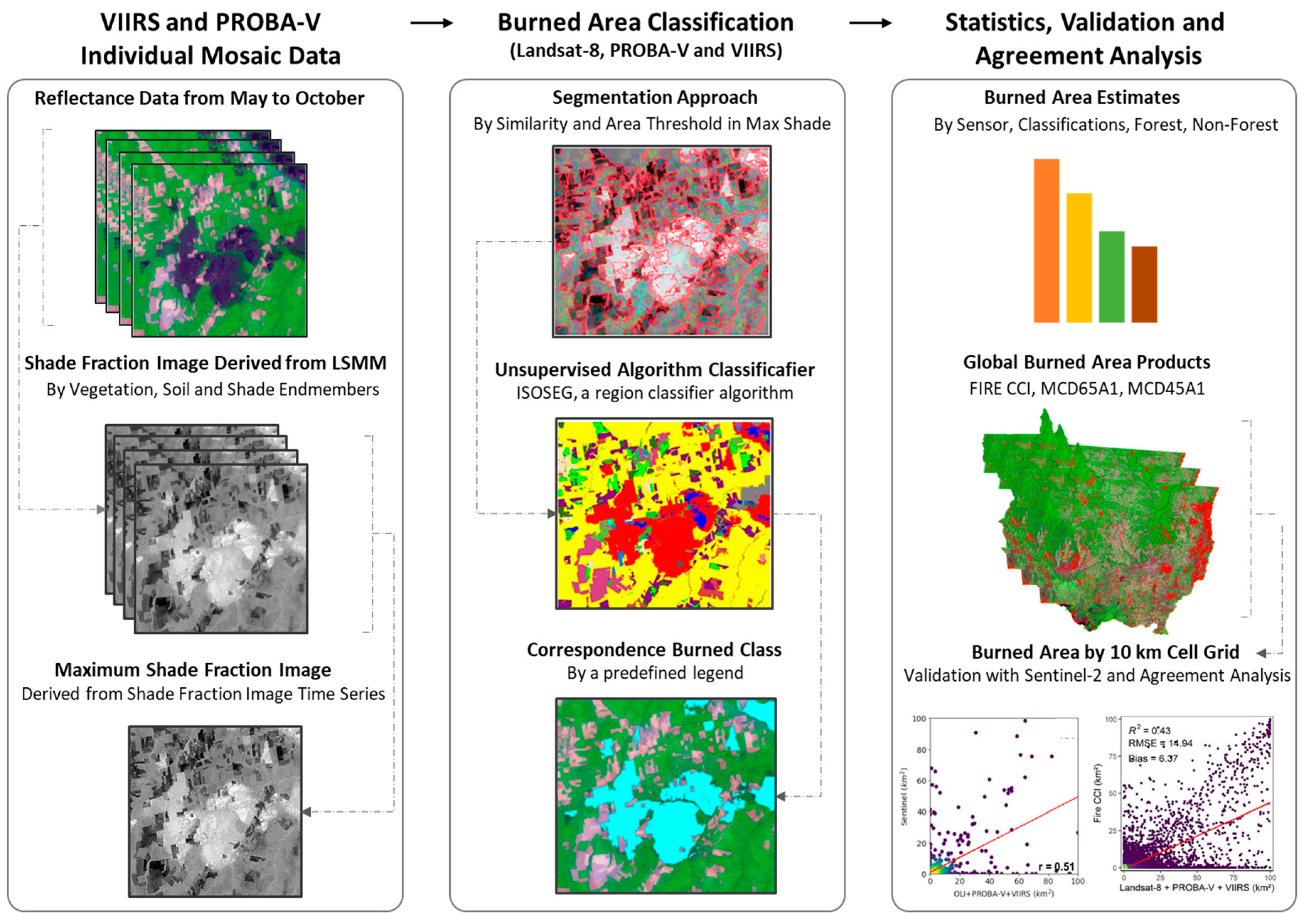
2.6. Methodological Overview

The Linear Spectral Mixing Model (LSMM) was applied to those remote sensors datasets to generate the vegetation, soil, and shade fraction images based on the three pure pixels adopted by Arai et al. [58]. The LSMM assumes that pixel values are linear combinations of reflectance from different components, called endmembers (Equation (1)). The resulting images are the proportion or fraction of each endmember in each pixel [59] (Figure 3).

$$r_i={\sum }_{j=1}^m{x}_j{a}_{i,j}+e_i,$$

(1)

where: r_i = the spectral reflectance in the ith spectral band; a_i,j = the spectral reflectance of the jth component (endmember) in the ith spectral band; x_j = the proportion of the jth component within the pixel; i = 1, …, n (number of spectral bands used); j = 1, …, m = 3 (number of considered components); and e_i = the residue for the ith spectral band.

The generation of these synthetic images is an alternative approach to reduce the dimensionality of image data and to enhance specific information (in this case, burned areas) for digital interpretation. Using the fraction images derived from the LSMM, a single image is composed containing the maximum proportion values of the shade fraction time series, comprising the burned areas information for PROBA-V and VIIRS datasets. This step was not applied to OLI images due to single images mosaic analyzed for the period.

Burned areas were obtained through digital classification of the shade fraction images using SPRING software [60] following a procedure based on image segmentation, unsupervised classification and assigning the corresponding classes to burned areas [61] for all sensor data (OLI, PROBA-V, and VIIRS) (Figure 4).

Image segmentation is a technique for grouping spatial information, whereby the algorithm assembles regions with and similar spectral characteristics. We used a region growing algorithm to perform the image segmentation. In such technique, two threshold parameters have to be set by the analyst to define segments (regions) at the subsequent classification procedure: (1) similarity threshold (the Euclidean distance between two regions with a different mean digital number of spectral clusters); and (2) an area threshold (the minimum area to be considered as a region, set by the number of pixels) [62]. In this work, the similarity and area thresholds were defined according to the sensors’ characteristics, as (8, 100), (8, 10), and (8, 4) for Landsat-8 OLI, PROBA-V, and VIIRS, respectively. Segmented images were classified using ISOSEG [62], a region classifier algorithm based on clustering techniques. This unsupervised algorithm uses the covariance matrix and the mean of the spectral values to estimate the centers of the classes in each region. The analyst defines an acceptance threshold, and the maximum allowed Mahalanobis distance that a mean digital number may be from the center of a class, considered as belonging to that class. The algorithm classifies the segments and separates them by classes based on the mentioned parameters. After the classification process and based on visual inspection, the labeling process is carried out only once, where all obtained classes from unsupervised classification were visually defined into classes with a real legend. This method was applied to the single shade fraction mosaic to obtain a final burned area classification for each sensor (PROBA-V, VIIRS, and OLI).

The final result is the mosaic of the burned area obtained from the three individual sensors. To show the visual consistency, a composite image was made highlighting the burned areas in the images of the three sensors; that is, the mapped burning pixels correspond to the original images of the sensors in which these areas were mapped. The burned areas were then calculated for the four results, including OLI, PROBA-V, NPP-VIIRS, and the final composite between the three products (OLI+PROBA-V+VIIRS). In addition, the burned area map obtained by the proposed method was superimposed on a PRODES and cropland datasets in order to analyze the spatial distribution and estimates of burned areas in the land use and land cover classes of the study area.

2.7. Evaluation and Agreement Analysis

In order to delineate burned areas in this study, 381 randomly distributed points in Sentinel-2 granules that included images from the period analyzed were used to estimate ground truth burned area, according to Equation (2):

$$Sample Size= \frac{N{z}^{2}p\left(1-p\right)}{\left(N-1\right)e^2+z^{2}p\left(1-p\right)},$$

(2)

where: N is the population size, z is the confidence level (95%) from Z-score, e is the margin of error (5%), and p is the sample proportion (50%). Afterward, we used the Goodness of Variance Fit (GVF) to cluster the Sentinel-2 MSI granules statistics (Equation (3)) [63]:

$$GVF= \frac{\left({\sum }_{i=1}^O{\left(x_i-\mu \right)}^2\right)-\left({\sum }_{c=1}^S{\sum }_{i=1}^O{\left(x_i-{\phi }_c\right)}^2\right)}{{\sum }_{i=1}^O{\left(x_i-\mu \right)}^2},$$

(3)

where: O is the Sentinel-2 MSI granules, $x_i$ is the sum of points inside the Sentinel-2 MSI granules, $\mu$ is the observations average, ${\phi }_c$ is the average of points over all granules, and S is the delimited classes in the optimization process. The clustering process separated the Sentinel-2 MSI granules in 2 groups, according to the density of random points (high and low), thus, burned areas were manually estimated in high density sampled granules (21LTC, 21LTE, 21LTG, 21LUC, 21LUD, and 21LUG).

Therefore, the burned areas derived from S2 MSI (considered the reference), Landsat-8 OLI, PROBA-V, Suomi NPP-VIIRS, and OLI+PROBA-V+VIIRS and the MCD45A1, MCD64A1, and Fire CCI global products were separated in several hexagonal grid cells with 10 km. This approach avoids the misregistration on the calculation of proportional errors for burned areas block sizes, and the bias in burned area estimation present in coarse and medium resolution burned area maps [34,64]. Then, a convolution mask was performed to estimate the agreement between products (Equation (4)).

$$B{A}_{\left(x,y.BAS,BAPi\right)}= {\sum }_{a=-\alpha }^{\propto }{\sum }_{b=-\beta }^{\beta }C\left(a,b\right).BAS\left(x+a,y+b\right) \cap C\left(a,b\right).BAPi\left(x+a,y+b\right),$$

(4)

where C(a,b) represents the convolution mask of M × N size (rows × columns); BAS is the burned areas estimated from Sentinel-2 data; BAPi is the burned areas estimated from burned areas products; and BA is the resulting grid defined for all points which the mask of M x N size completely overlaps the grid (x ϵ (α, M −α), y ϵ (β, N −β)).

The agreement analysis considered the same hexagonal grid cell of the evaluation analysis. We computed the proportion of burned areas of the auxiliary global burned area data products (MCD45A1, MCD64A1, and Fire CCI) and counted active fire observations by the presence or absence in each cell compared with the four results (OLI, PROBA-V, NPP-VIIRS, and OLI+PROBA-V+VIIRS). Based on these data, it was calculated the determination coefficient (r²), root-mean-square error (RMSE), and bias.

3. Results

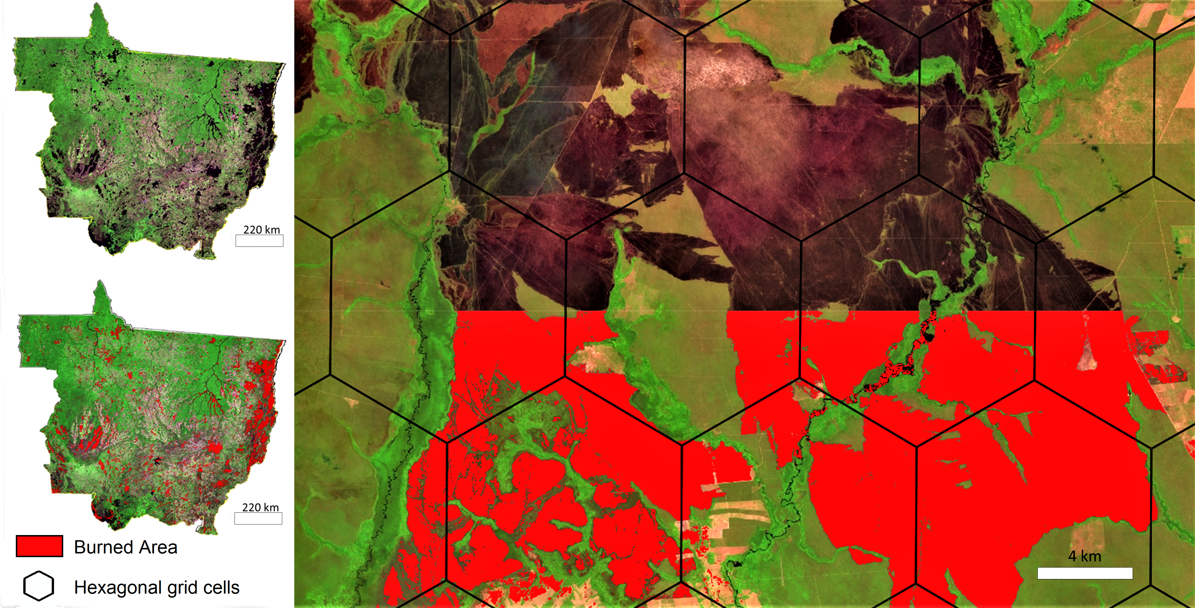
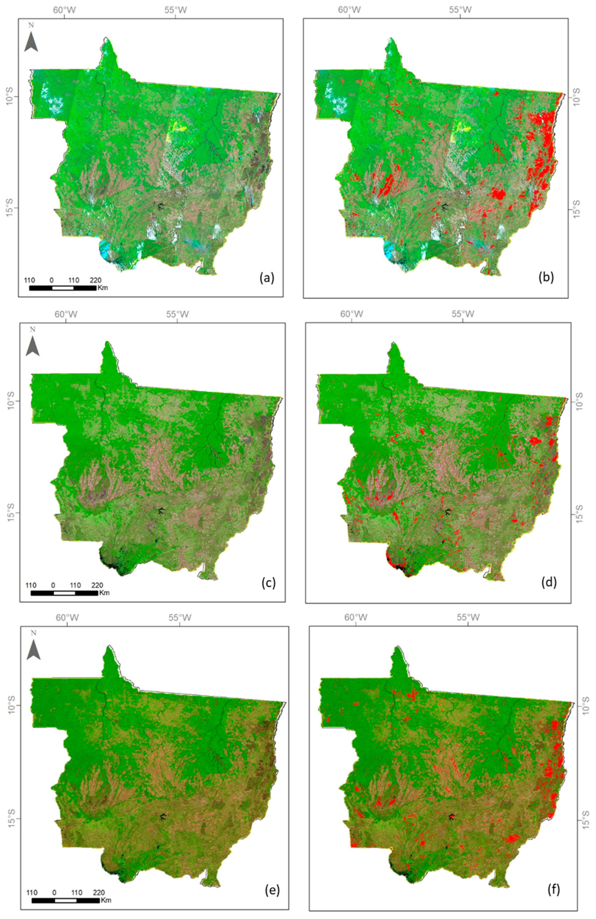
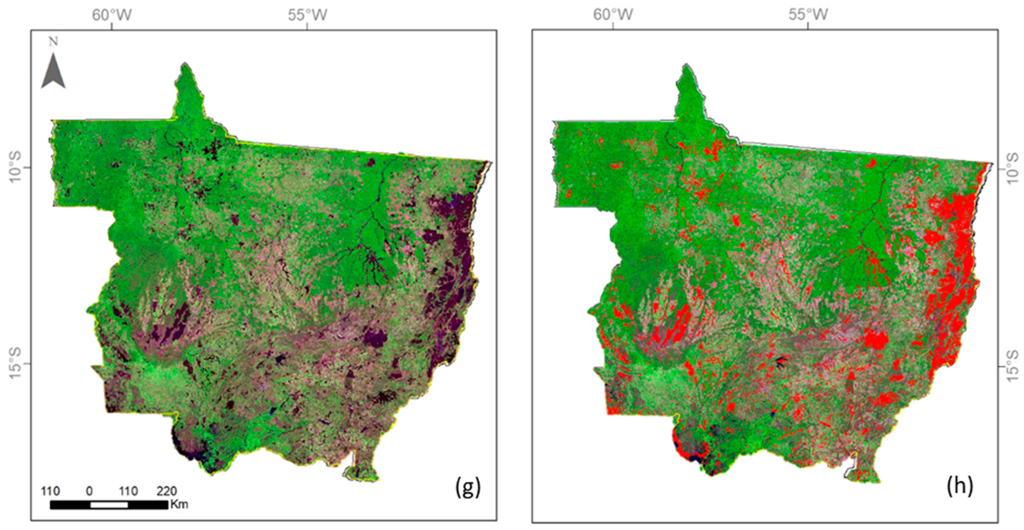
3.1. Burned Area Spatial Distribution and Estimates by Land Cover

The total burned area mapped from each sensor and by the final composite is showed in Figure 5b,d,f. It is important to highlight that burned areas results were obtained during the dry season and appear in dark color from the RGB mosaic in Figure 5a,c,e. A total of 55,694.32 km² of the burned area mapped by OLI sensor represents 6.15% of the study area, followed by VIIRS sensor with 29,768.72 km² of the burned area (3.28% of the study area); the PROBA-V sensor with 28,443.52 km² (3.14%); and then 93,027.92 km² (10.27%) mapped by the final composite (Figure 5h).

The estimates of burned areas superimposed on the PRODES and cropland datasets are shown in

Table 2. Estimated burned areas in deforested areas, forest, non-forest, and cropland areas using the final composite mapping.

Classes of Land Cover	Burned Area (km2)	Total Burned Area (%)
2015 Deforestation	786.15	0.86%
Old Deforestation	19,745.43	21.54%
Non-Forest	61,009.31	66.57%
Forest	10,111.04	11.03%
Cropland	4873.32	5.32%

. The results pointed out that the most burned area estimate is located in non-Forest, reaching 66.57% (~61 thousand km²) of the total area mapped by the final composite. Deforested areas, characterized by old (before 2015) and recent clear-cuts (2015 year), presented 21.54% (~19 thousand km²) and 0.86% (~786 km²), respectively. The results also showed less burn in croplands (5.32%, representing ~4 thousand km²) than in forested areas (11.03%, ~10 thousand km²).

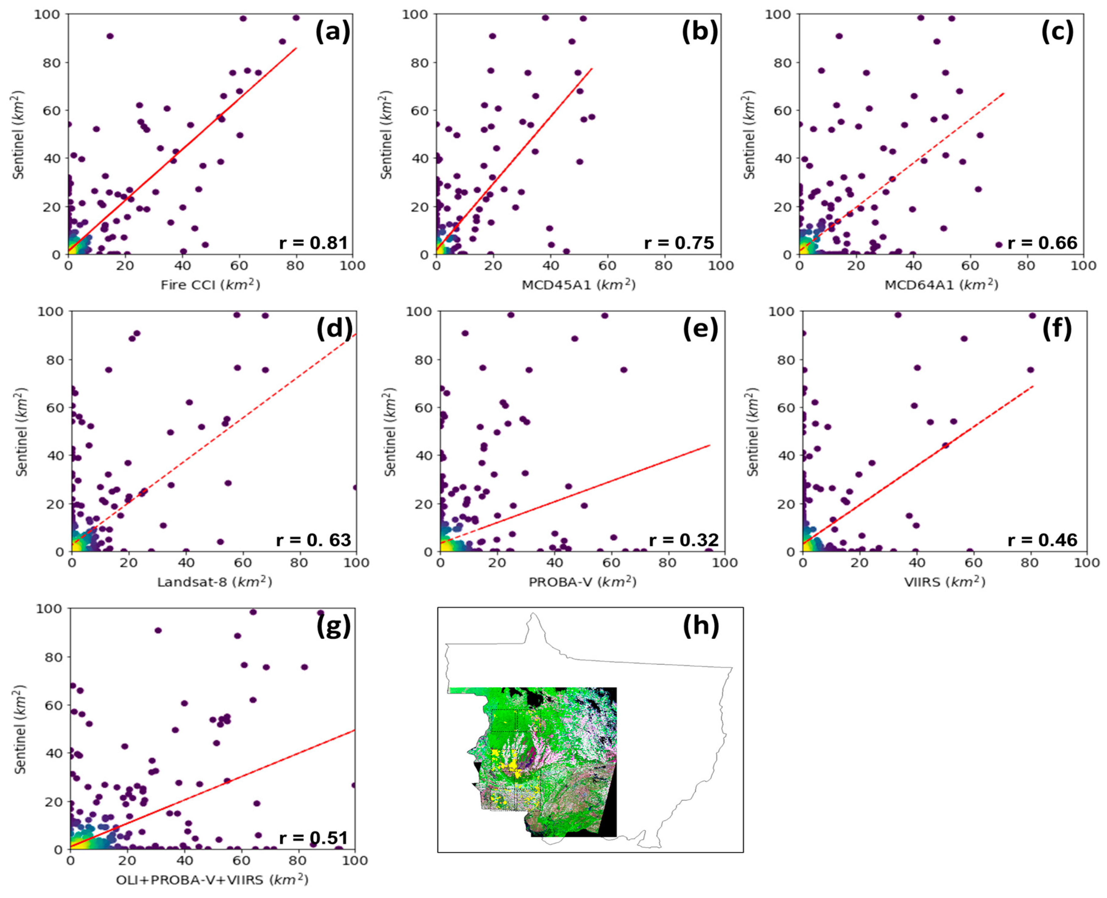
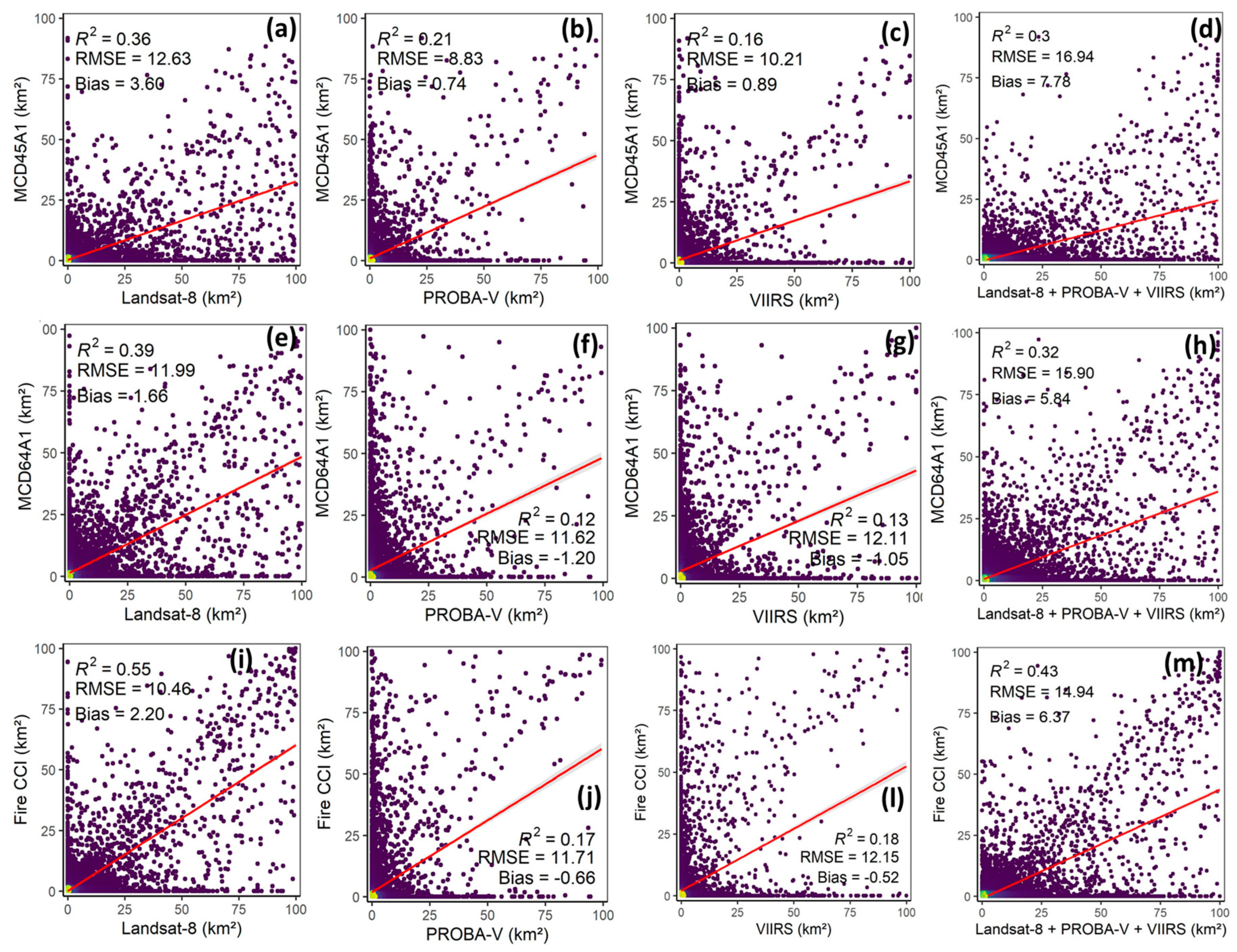
3.2. Evaluation and Agreement Analysis

Figure 6 shows the evaluation graphics of burned areas maps for 6 granules (21LTC, 21LTE, 21LTG, 21LUC, 21LUD, and 21LUG) of S2 MSI reference data. It is noticed that the correlations vary according to the products and with burned areas size and location. The lower values ranged between 0.32 and 0.63 and the highest values ranged between 0.66 and 0.81 (all linear regressions were significant at p < 0.05, Student t-test). In the Sentinel-2 MSI burned areas, approximately 84% of grid cells had values lower than 5 km², with 41 hexagonal grid cells greater than 30 km². This indicates that burned area patterns correspond to small scars (as shown in density scatter plot of Figure 6a–g).

In analyzed products, we found several commission areas related mainly to dark red latosol, relief shading and water bodies that were not mapped in reference data. In these areas, where no burned scars occur, Fire CCI, MCD45A1, MCD64A1, Landsat-8 OLI, PROBA-V, NPP-VIIRS, and OLI+PROBA-V+VIIRS presented an inclusion of 150 km², 108 km², 488 km², 282 km², 930 km², 484 km², and 1712 km², respectively. Otherwise, we can find several hexagonal grid cells where burned areas were presented and fire products were unable to estimate (464 km², 550 km², 386 km², 547 km², 437 km², 1240 km², and 126 km² to Fire CCI, MCD45A1, MCD64A1, Landsat-8 OLI, PROBA-V, NPP-VIIRS, and OLI+PROBA-V+VIIRS, respectively).

Figure 7 compares only grid cells containing burned area between the results obtained by the proposed method (OLI+PROBA-V+VIIRS, OLI, PROBA-V, and NPP-VIIRS) with the available global datasets (MCD64A1, MCD45A1, and Fire CCI). There is a good visual agreement among the results from the four datasets, highlighted in a majority on the eastern Mato Grosso State, encompassing the Cerrado biome, and west, encompassing the Amazon biome. In the middle of the state, most cells in the grid contain only one or two global products with an agreement with the results of our method. The analysis based on active fire observation showed that most cells with the total agreement of burned detected by our method and global products present the highest number of active fire observations (from 51 to 133), being decreased when less agreement occurs.

The analysis with active fire observations showed an agreement of 92.08% compared with the final composite burned area classification obtained using the proposed method in terms of the presence of active fire and burned area detection (

Table 3. Percentages of grid cells compared by burned area detection and active fire observations.

Product	Active Fire and Mapped (%)	Non-Active Fire and Mapped (%)	Non-Active Fire and Non-Mapped (%)	Active Fire and Non-Mapped (%)
OLI+PROBA-V+VIIRS	92.08	72.73	27.27	7.92
OLI	71.97	44.44	55.56	28.03
PROBA-V	68.08	51.27	48.73	31.92
NPP-VIIRS	34.17	24.89	75.11	65.83
MCD64A1	64.57	16.43	83.57	35.43
MCD45A1	41.47	14.92	85.08	58.53
Fire CCI	51.89	8.79	91.21	48.11

). Compared with OLI, PROBA-V, and VIIRS, the agreement percentage decreases when lower the spatial resolution, with OLI sensor presenting the best result (71.97%) and VIIRS the lowest comparison (34.17%). Related to commission errors, where there is a burned area detected but no active fire observed, PROBA-V produced the highest commission error (51.27%), while the Fire CCI data had the lowest (8.79%).The omission errors (active fire detected and no burned area mapped) resulted in the best results for OLI sensor (28.03%) and the highest omission for VIIRS sensor (65.83%). Overall, the final composite classification (OLI+PROBA-V+VIIRS) results showed lower omission error (7.92%) but a higher commission error (72.73%) than all analyzed datasets.

There were substantial differences in mapped areal extent of burned areas across the various datasets (

Table 4. Burned area estimated by the proposed method and by the global burned area products.

Product	Area (km2)
OLI+PROBA-V+VIIRS	96,461.24
OLI	55,694.32
PROBA-V	28,443.52
NPP-VIIRS	29,768.72
MODIS MCD64A1	40,364.75
MODIS MCD45A1	31,555.25
Fire CCI	34,991.13

). Our results are overestimated compared with MCD64A1, MCD45A1, and Fire CCI datasets, respectively. However, these overestimates decrease when compared with individual sensor datasets.

Figure 8 shows the regression analysis of burned areas maps for each sensor and final composite compared with the global burned areas products by cell grid. Compared with the final composite, it was obtained that r² = 0.30 for MCD45A1, r² = 0.32 for MCD64A1, and r² = 0.43 for Fire CCI (Figure 8d,e,m, respectively). The RMSE varies from 16.94 to 14.94, and the bias between 7.78% to 5.84%. RMSE measures indicate a generally better spatial agreement between the products when the results are lower, being used as an indicator of the dispersion or tendency of classifiers to identify the same amount of burned areas across cells. However, the lack of bias in the regression model not necessarily has the same indicative [34]. In this case, the bias showed to be positive, and, as mentioned before, the final composite has a trend to overestimate the results compared with the global burned area products.

The regression results between the global burned area products and the burned areas mapped by each sensor showed Landsat-8 OLI with the best results (from r² = 0.55 to r² = 0.36), followed by PROBA-V (from r² = 0.21 to r² = 0.12) and NPP-VIIRS (from r² = 0.18 to r² = 0.13). The RMSE values were around 12.63, as observed with MCD45A1 and Landsat-8 OLI (Figure 8a), and 8.83 in MCD45A1 and PROBA-V (Figure 8b). The bias also showed to be positive for the most analysis, around 3.60% in MCD45A1 and Landsat-8 OLI (Figure 8a) and 0.74% in MCD45A1 and PROBA-V (Figure 8b), representing an overestimation. On the other hand, as observed previously, the mapped burned areas of PROBA-V and NPP-VIIRS sensors were underestimated when compared with MCD64A1 and Fire CCI products, representing a negative bias around to 1.20% in MCD64A1 and PROBA-V (Figure 8f) to 0.52% in Fire CCI and NPP-VIIRS (Figure 8l).

4. Discussion

4.1. Burned Area by Land Cover

Historically, fire has been the main tool in the land use and land cover changes, and the impacts of fires on the environment, especially on the climate, require the analysis and monitoring of large territorial extensions in the long term. In a total of approximately of 96,461.24 km² of the burned areas identified in the Mato Grosso State, our results indicate that 66% of the total burned area occurs in non-forested areas, including savanna formations and grasslands, mainly founded in the Cerrado and Pantanal biomes. Twenty-one percent and 0.86% of burned areas were identified in older deforestation (before the 2015 year) and in deforested areas identified in the same year by the PRODES dataset, respectively. Critically, forested areas experienced 11% of the total burned area, and the occurrence of fires in forest formations can have negative social, economic, and environmental consequences, also favoring the conversion to deforestation. Additionally, the most effective policy instruments in reducing deforestation are not the most effective in reducing forest fires and vice-versa, suggesting that both objectives cannot be achieved with a single measure of political intervention [65]. In this manner, Brazilian government policies still need to be rethought to contemplate the reduction of forest fires and the mitigation of their negative effects.

4.2. Overall Accuracy and Agreement Analysis

Although using the same MODIS sensor datasets, the existing global burned areas (Fire CCI, MCD45A1, and MCD64A1) products present different results. These differences are due to the methodologies and image dates used to generate such products. Our proposed method used image datasets from OLI, PROBA-V, and VIIRS sensors with different temporal and spatial resolutions. Then, we generated different results using these sensors datasets individually. We also generated a composite result by adding those individual results taking the advantages of higher temporal resolution of PROBA-V and VIIRS sensors and the medium spatial resolution of Landsat-8 OLI sensor. The results showed a good visual agreement among all burned areas maps produced by different sensors datasets and methodologies. However, the areal extents of burned areas were very different.

The proposed method used to generate the burned areas maps in this study showed different results according to the sensor analyzed. When evaluated with the reference data (Sentinel-2 MSI), the OLI sensor presented the best correlation (r = 0.63), followed by VIIRS (r = 0.46) and PROBA-V (0.32). In this context, the spatial resolution of OLI sensor (30 m) could explain the highest correlation. This analysis is corroborated by Reference [64], where the authors cite that a key determinant on the accuracy of burned area detection is the spatial mapping scale of dataset, with evidence that burned area maps produced from higher resolution observations presented reduced omission errors.

Although PROBA-V has better spatial resolution than VIIRS (100 m and 500 m, respectively), both presented similar results. The clouds and shadows were removed in the two products before the mapping, and the temporal analysis was the same (from May to October months). Therefore, the number of images utilized may explain the difference in results since VIIRS sensor is a daily product, compared to the composite of 5-days for PROBA-V, totalizing 153 and 36 images, respectively. Thus, some fires could be missed in PROBA-V, impacting in the evaluation process.

In relation to the evaluation using Sentinel-2 MSI data to delimited the burned area by visual interpretation, it is important to notice that the period analyzed (August to November) not coincide with PROBA-V and VIIRS dataset used in this study (May to November). Moreover, only a segment of Mato Grosso State was observed. Both limitations are related to the number of available images in 2015, due to the launch date (June 2015) of Sentinel-2A, which may cause uncertainties in the evaluation.

When comparing the reference data with the global burned area products, the Fire CCI, MCD45A1, and MCD64A1 presented a better correlation than OLI sensor, with a better agreement to Fire CCI (0.81), followed by MCD45A1 (0.75) and MCD64A1 (0.66). The number of scenes used to map the burned areas in OLI sensor may explain these results. Due to the persistency of clouds, some scenes could not be used and, in general, only one date was mapped for each of the 47 path/rows that comprise the state of Mato Grosso, most of them in October, missing some burned areas. In addition, the slightly better correlation of MCD45A1 compared to the MODIS improved product MCD64A1 may be related to the lower commission error presented by MCD45A1 (108 km²) compared to MCD64A1 (488 km²). Still, the final product OLI+PROBA-V+VIIRS not presented a good correlation (0.51), even when compared to OLI.

4.3. Specific Product of Burned Area by Each Dataset

The OLI sensor presented the highest values of the total burned area, with 55,694 km², followed by VIIRS and PROBA-V (29,768 km² and 28,443 km², respectively). As mentioned before, the better spatial resolution of OLI sensor could be a factor in detecting more burned areas, as well as the largest number of scenes used of VIIRS sensor. The OLI sensor resulted in the most total burned areas mapped comparing these results with global burned areas products, followed by Fire CCI product (34,991 km²) and MCD64A1 (31,555 km²). The better spatial resolution of Fire CCI (250 m) could be related to more burned areas detected and, according to Reference [34], Fire CCI and MCD64A1 are efficient in identifying burned area in cloudy regions due to their reliance on active fire detections as training data samples. PROBA-V presented the lowest burned area mapped, which may be linked to the number of scenes used when compared to the OLI+PROBA-V+VIIRS final product.

The spatial resolution of OLI could also explain the best results of this sensor related to commission errors (282 km²), followed by VIIRS and PROBA-V (484 km² and 930 km², respectively). In Mato Grosso State, some elements may be confused with burned areas, like the presence of dark red latosol, especially in agricultural areas where they are most exposed. Cloud shadows, topographic shadowing, and water bodies have similar spectral characteristics as burned areas. According to Reference [66], other features that can be confused with the burned areas include clear cuts, land conversion, and non-fire forests mortality. Compared with the global burned area products, PROBA-V presented the highest commission error value, followed by MCD64A1 (488), VIIRS (484), OLI (282), Fire CCI (150), and MCD45A1 (108). The lowest commission error of burned areas by MCD45A1 could be explained by high omission error from this product, as will be mentioned later.

Related to omission errors, OLI and PROBA-V presented similar results, with 547 km² and 437 km², respectively. The number of scenes used to map the burned areas may explain the slight increase in the omission error of OLI sensor. The VIIRS sensor presented the highest omission error of burned area (1240 km²), and, when compared to OLI and PROBA-V, the 500 m spatial resolution of the product may explain the differences, since approximately 84% of the burned areas found in reference data is composed by scars with less than 5 km². According to Reference [64], sensors with moderate and coarse spatial resolution presents a low degree of fidelity in the detection of small or highly fragmented fires. Besides, omissions can also occur when fires leave little residual heat and spread rapidly between satellite overpasses and when the differences in the spectral characteristics between pre- and post-fire are minimal [67]; and, to Reference [68], fires obscured by clouds, with short-lived thermal signatures and small fires also may not be identified.

Compared with the global burned area products, the VIIRS sensor resulted in higher omission error of burned area, followed by OLI (547 km²), MCD45A1 (550 km²), Fire CCI (464 km²), PROBA-V (437 km²), MCD64A1 (386 km²), and OLI+PROBA-V+VIIRS final product (126 km²). The OLI product showed a high rate of fires omission (ranking second). Thus, the temporal resolution is also crucial in the analysis and identification of burned areas, avoiding non-identification throughout the season. Related to global burned area products, the MCD64A1 presented the best performance, mostly due to the improvement in the algorithm, that integrates reflectance changes with active fire observations. Several validation studies for global products have identified the good performance of MCD64A1 in the identification of burned areas with low errors of omission [34,69,70]. Finally, the combined results of the proposed method presented the lowest omission of burned areas, indicating that the combination of higher temporal and medium spatial resolution could be a better approach to identifying burned areas.

4.4. Comparison with Active Fires

When comparing the final classification of burned areas with the active fire observations, it is noticed that related to omissions (active fires detected but not-mapped), the final composite product (OLI+PROBA-V+VIIRS) presented the best performance (7.92%), followed by OLI (28.03%), PROBA-V (31.92%), MCD64A1 (35.43%), Fire CCI (48.11%), MCD45A1 (58.53%), and VIIRS (65.83%). Therefore, sensors that present better spatial resolution and products with algorithms that use active fires present the best results. In this context, MCD45A1, that uses only reflectance images, and VIIRS, both with 500 m of spatial resolution, did not detect more than half of the burned areas even with active fires occurring.

Related to commission (burned area mapped with no active fire detected), Fire CCI presented the best performance (8.79%), indicating that the 250 m spatial resolution with the use of active fire product is efficient in not including burns that do not exist, or that may exist but are characterized by small scars where active fires are absent. The next following products presented the best results: MCD45A1 (14.92%), MCD64A1 (16.43%), VIIRS (24.89%), OLI (44.44%), PROBA-V (51.27%), and OLI + PROBA-V + VIIRS (72.73%). In this context, MCD45A1 and VIIRS that presented high values of omission errors related to active fires also presented low values of commission errors, the same pattern demonstrated by OLI + PROBA-V + VIIRS, that presented the best performance related to omission error and lowest performance related to commission errors.

The last analysis is related to the burned areas mapped that presented active fires. The OLI+PROBA-V+VIIRS product presented the best performance (92.08%), followed by OLI (71.97%), PROBA-V (68.08%), and MCD64A1 (64.57%). Besides, Fire CCI presents better spatial distribution compared to MCD64A1, and this product presented 51.89% of burned areas mapped in areas with active fires, followed by MCD45A1 (45.47%) that do not use active fires in the algorithm to map the burned areas. The sensor with the worst performance was VIIRS, with 34.17% of burned areas mapped, indicating that the 500 m spatial resolution does not perform well in areas with small burn scars, even with active fires.

In this context, the algorithm accuracies can be influenced by fire patch characteristics, since small and irregular burned area patches may lead to high omission errors because the spatial resolution of the pixels is too coarse to detect the smaller fires [71]. On the other hand, small and irregular unburned areas within large burned patches may lead to an increase in commission errors, particularly for high sensitivity algorithms [57].

In the Amazon biome, the burning activity is performed to clean newly deforested areas for agriculture expansion, and sometimes the fires escape to forest areas causing forest degradation. Nevertheless, these remaining areas contain less biomass and are not considered in the carbon balance yet. In non-forested areas, burnings are caused by the use of fire to improve the productivity of grassland and pastureland covers. In this context, previous validation studies have indicated that global satellite-derived burned area products typically perform best in regions where fire activity is more prevalent [69], and, for South America, Reference [70] found that the smallest relative uncertainties occur in the frequently burning savannas and grasslands.

5. Conclusions

The use of remote sensing burned areas products requires confident estimates uncertainties. Therefore, in this paper, a method combining products with higher spatial and temporal resolutions to estimate the burned areas, by using OLI, PROBA-V, and NPP-VIIRS datasets, was proposed. The shade fraction images showed the advantages to reduce the data volume to be analyzed and highlighting the burned areas facilitating the image classification process, even with a high volume of data. In the study area, 11% (10,111 km²) of burnings occurred in forested areas, reaching the double of burned area extension compared with areas destined for agriculture (5%, 4873 km²). This indicates that fire occurrences are less in areas intended for agriculture using mechanized practices, although it is still a common practice due to its low cost and cultural habits. On the other hand, Brazilian government policies still need to be rethought to contemplate the reduction of forest fires and the mitigation of their negative effects.

Regarding to the total burned area, the 30 m high spatial resolution of OLI sensor resulted in the best results and the less commission errors; however, when evaluated with reference data (Sentinel-2 MSI), the Fire CCI global burned area product presented the best correlation, and this fact can be explained by the persistency of clouds in Mato Grosso State of 2015 year, resulting in less available images of OLI sensor, indicating the crucial importance of temporal resolution in burned areas analysis.

The final product OLI+PROBA-V+VIIRS used by the proposed method overestimated the burned areas and presented a moderate correlation compared to the reference data; however, it presented the lowest omission of burned areas and the best performance related to the mapping of burnings in areas with active fire observations. Therefore, these results indicate that the combination of higher temporal and medium spatial resolutions sensor data could be a better approach to identifying burned areas, since the best spatial resolution is indicated to small scars identification and high temporal resolution is used to avoid omission errors. In this context, the temporal resolution is also extremely important, being necessary the use of all scenes available, and a cloud mask could assist in the use of images that have a longer revisit period, improving the results obtained. For future studies, the recommendation is to use a machine learning algorithm and cloud processing for monitoring burned areas using different datasets and a high volume of data for larger areas. In addition, using ancillary information, e.g., water bodies map, may avoid the confusion of burned areas and water bodies and, consequently, improve the classification process.

The proposed method provided a general perspective about the patterns of fire in the Amazon, Cerrado, and Pantanal biomes of Mato Grosso State, Brazil, discriminating by forestland, cropland, and deforested and non-forested areas. Such information is important for environmental studies, especially related to fire severity, regeneration, and greenhouse gas emissions.

References

1. Belcher, C.M. Fire Phenomena and the Earth System: An Interdisciplinary Guide to Fire Science; College of Life and Environmental Sciences, University of Exeter: Exeter, UK, 2013. [Google Scholar]
2. Coutinho, L.M. Fire in the ecology of the Brazilian cerrado. In Fire in the Tropical Biota; Goldammer, J.G., Ed.; Springer-Velarg: New York, NY, USA, 1990; pp. 82–105. [Google Scholar]
3. Alencar, A.; Nepstad, D.; Silva, E.; Brown, F.; Lefebvre, P.; Mendosa, E.; Almeida, D.; Carvalho, O., Jr. Uso do Fogo na Amazônia: Estudos de Caso ao Longo do Arco de Desmatamento; World Bank Report; World Bank: Brasilia, Brazil, 1997. [Google Scholar]
4. Sampaio, G.; Nobre, C.; Costa, M.H.; Satyamurty, P.; Soares Filho, B.S.; Cardoso, M.F. Regional climate change over eastern Amazonia caused by pasture and soybean cropland expansion. Geophys. Res. Lett. 2007, 34, 1–7. [Google Scholar] [CrossRef] [Green Version]
5. Marengo, J.A.; Nobre, C.; Salazar, L.F. Regional climate change cenarios in South America in the Late XXI Century: Projections and expected impacts. Nova Acta Leopoldina 2010, 112, 251–265. [Google Scholar]
6. Bustamante, M.M.C.; Roitman, I.; Aide, T.M.; Alencar, A.; Anderson, L.; Aragão, L.; Asner, G.P.; Barlow, J.; Berenguer, E.; Chambers, J.; et al. Towards an integrated monitoring framework to assess the effects of tropical forest degradation and recovery on carbon stocks and biodiversity. Global Change Biology 2016, 1, 92–109. [Google Scholar] [CrossRef] [PubMed]
7. Cochrane, M.A.; Ryan, K.C. Fire and fire ecology: Concepts and principles. In Tropical Fire Ecology, Climate Change, Land Use and Ecosystem Dynamics; Cochrane, M.A., Ed.; Springer: Chichester, UK, 2009; pp. 60–97. [Google Scholar] [CrossRef]
8. Freitas, S.R.; Longo, K.M.; Dias, M.A.F.S.; Dias, P.L.S.; Chatfield, R.; Prins, E.; Artaxo, P.; Grell, G.A.; Recuero, F.S. Monitoring the transport of biomass burning emissions in South America. Environ. Fluid Mechanics 2005, 5, 135–167. [Google Scholar] [CrossRef]
9. Fearnside, P.M.; Righi, C.A.; Graça, P.M.L.A.; Keizer, E.W.H.; Cerri, C.C.; Nogueira, E.M.; Barbosa, R.I. Biomass and greenhouse gas emissions from land-use change in Brazil’s Amazonian ‘‘arc of deforestation’’: The states of Mato Grosso and Rondônia. Forest Ecology Manag. 2009, 258, 1968–1978. [Google Scholar] [CrossRef]
10. Leblon, B.; Bourgeau-Chavez, L.; San-Miguel-Ayanz, J. Use of Remote Sensing in wildfire management. In Sustainable Development–Authoritative and Leading Edge Content for Environmental Management; Curkovic, S., Ed.; InTech Press: Rijeka, Croatia, 2012; pp. 55–82. [Google Scholar]
11. Tyukavina, A.; Hansen, M.C.; Potapov, P.V.; Stehman, S.V.; Smith-Rodriguez, K.; Okpa, C.; Aguilar, R. Types and rates of forest disturbance in Brazilian Legal Amazon, 2000–2013. Science Advances 2017, 3, e1601047. [Google Scholar] [CrossRef] [Green Version]
12. Davidson, E.A.; De Araüjo, A.C.; Artaxo, P.; Balch, J.K.; Brown, I.F.; Mercedes, M.M.; Coe, M.T.; Defries, R.S.; Keller, M.; Longo, M.; et al. The amazon basin in transition. Nature 2012, 481, 321–328. [Google Scholar] [CrossRef]
13. Cardozo, F.S.; Pereira, G.; Shimabukuro, Y.E.; Moraes, E.C. Analysis and Assessment of the Spatial and Temporal Distribution of Burned Areas in the Amazon Forest. Remote Sensing 2014, 6, 8002–8025. [Google Scholar] [CrossRef] [Green Version]
14. Stephenson, C.; Handmer, J.; Betts, R. Estimating the economic, social and environmental impacts of wildfires in Australia. Environ. Hazards 2013, 12, 93–111. [Google Scholar] [CrossRef]
15. Van der Werf, G.R.; Randerson, J.T.; Giglio, L.; Collatz, G.J.; Kasibhatla, P.S.; Arellano, A.F., Jr. Interannual variability in global biomass burning emissions from 1997 to 2004. Atmos. Chem. Phys. 2006, 6, 3423–3441. [Google Scholar] [CrossRef] [Green Version]
16. Andreae, M.O. Biomass burning: Its history, use, and distribution and its impact on environmental quality and global climate. In Global Biomass Burning: Atmospheric, Climatic, and Biospheric Implications; Levine, J.S., Ed.; The MIT Press: Cambridge, MA, USA, 1991; pp. 2–21. [Google Scholar]
17. Durigan, G.; Ratter, J.A. The need for a consistent fire policy for Cerrado conservation. J. Appl. Ecol. 2016, 53, 11–15. [Google Scholar] [CrossRef]
18. Mataveli, G.A.V.; Silva, M.E.S.; Pereira, G.; Cardozo, F.S.; Kawakubo, F.S.; Bertani, G.; Costa, J.C.; Ramos, R.C.; Silva, V.V. Satellite observations for describing fire patterns and climate-related fire drivers in the Brazilian savannas. Nat. Hazards Earth Syst. Sci. 2018, 18, 125–144. [Google Scholar] [CrossRef] [Green Version]
19. Ichoku, C.; Kahn, R.; Chin, M. Satellite contributions to the quantitative characterization of biomass burning for climate modeling. Atmos. Res. 2012, 111, 1–28. [Google Scholar] [CrossRef] [Green Version]
20. Justice, C.O.; Giglio, L.; Korontzi, S.; Owens, J.; Morisette, J.; Roy, D.; Descloitres, J.; Alleaume, S.; Petitcolin, F.; Kaufman, Y. The MODIS fire product. Remote Sens. Environ. 2002, 83, 244–262. [Google Scholar] [CrossRef]
21. Pereira, G.; Siqueira, R.; Rosário, N.E.; Longo, K.L.; Freitas, S.R.; Cardozo, F.S.; Kaiser, J.W.; Martin, J.; Wooster, M.J. Assessment of fire emission inventories during the South American Biomass Burning Analysis (SAMBBA) experiment. Atmos. Chem. Phys. 2016, 16, 6961–6975. [Google Scholar] [CrossRef] [Green Version]
22. Roy, D.P.; Lewis, P.E.; Justice, C.O. Burned area mapping using multi-temporal moderate spatial resolution data—a bi-directional reflectance model-based expectation approach. Remote Sens. Environ. 2002, 83, 263–286. [Google Scholar] [CrossRef]
23. Chuvieco, E.; Mouillot, F.; van der Werf, G.R.; Miguel, J.S.; Tanase, M.; Koutsias, N.; García, M.; Yebra, M.; Padilla, M.; Gitas, I.; et al. Historical background and current developments for mapping burned area from satellite Earth observation. Remote Sens. Environ. 2019, 225, 45–64. [Google Scholar] [CrossRef]
24. Coppoletta, M.; Merriam, K.E.; Collins, B.M. Post-fire vegetation and fuel development influences fire severity patterns in reburns. Ecol. Appl. 2016, 26, 686–699. [Google Scholar] [CrossRef]
25. Andrés, R.G.; Davies, G.M.; Waldron, S.; Scott, E.M.; Gray, A. Increased fire severity alters initial vegetation regeneration across Calluna-dominated ecosystems. J. Environ. Manag. 2019, 231, 1004–1011. [Google Scholar] [CrossRef] [Green Version]
26. Casady, G.M.; Marsh, S.E. Broad-scale environmental conditions responsible for post-fire vegetation dynamics. Remote Sens. 2010, 2, 2643–2664. [Google Scholar] [CrossRef] [Green Version]
27. Chen, Z. A literature Survey: The Effects of Forest Fire on Ecology and Regeneration. Ph.D. Thesis, Faculty of Forestry and the Forest Environment, Lakehead University, Thunder Bay, ON, USA, 2019; 43p. [Google Scholar]
28. Hantson, S.; Padilla, M.; Corti, D.; Chuvieco, E. Strengths and weaknesses of MODIS hotspots to characterize global fire occurrence. Remote Sens. Environ. 2013, 131, 152–159. [Google Scholar] [CrossRef]
29. Andela, N.; van der Werf, G.R.; Kaiser, J.W.; van Leeuwen, T.T.; Wooster, M.J.; Lehmann, C.E.R. Biomass burning fuel consumption dynamics in the tropics and subtropics assessed from satellite. Biogeosciences 2016, 13, 3717–3734. [Google Scholar] [CrossRef] [Green Version]
30. Loboda, T.; O’Neal, K.J.; Csiszar, I. Regionally adaptable dNBR-based algorithm for burned area mapping from MODIS data. Remote Sens. Environ. 2007, 109, 429–442. [Google Scholar] [CrossRef]
31. Roteta, E.; Bastarrika, A.; Padilla, M.; Storm, T.; Chuvieco, E. Development of a Sentinel-2 burned area algorithm: Generation of a small fire database for sub-Saharan Africa. Remote Sens. Environ. 2019, 222, 1–17. [Google Scholar] [CrossRef]
32. Schroeder, W.; Morisette, J.T.; Csiszar, I.; Giglio, L.; Morton, D.; Justice, C.O. Characterizing vegetation fire dynamics in Brazil through multisatellite Data: Common trends and practical issues. Earth Interact. 2005, 9, 1–26. [Google Scholar] [CrossRef] [Green Version]
33. Giglio, G.; Boschetti, L.; Roy, D.P.; Humber, M.L.; Justice, C.O. The Collection 6 MODIS Burned Area Mapping Algorithm and Product. Remote Sens. Environ. 2018, 217, 72–85. [Google Scholar] [CrossRef]
34. Humber, M.L.; Boschetti, L.; Giglio, L.; Justice, C.O. Spatial and temporal intercomparison of four global burned area products. Int. J. Digital Earth 2019, 12, 460–484. [Google Scholar] [CrossRef]
35. Hawbaker, T.J.; Vanderhoof, M.K.; Beal, Y.J.; Takacs, J.D.; Schmidt, G.L.; Falgout, J.T.; Williams, B.; Fairaux, N.M.; Caldwell, M.K.; Picotte, J.J.; et al. Mapping burned areas using dense time-series of Landsat data. Remote Sens. Environ. 2017, 198, 504–522. [Google Scholar] [CrossRef]
36. Cabral, A.I.R.; Silva, S.; Silva, P.C.; Vanneschi, L.; Vasconcelos, M.J. Burned area estimations derived from Landsat ETM+ and OLI data: Comparing Genetic Programming with Maximum Likelihood and Classification and Regression Trees. ISPRS J. Photogramm. Remote Sens. 2018, 142, 94–105. [Google Scholar] [CrossRef]
37. Chen, D.; Pereira, J.M.C.; Masiero, A.; Pirotti, F. Mapping fire regimes in China using MODIS active fire and burned area data. Appl. Geogr. 2017, 85, 14–26. [Google Scholar] [CrossRef]
38. Melchiorre, A.; Boschetti, L. Global Analysis of Burned Area Persistence Time with MODIS Data. Remote Sens. 2018, 10, 750. [Google Scholar] [CrossRef] [Green Version]
39. Urbanski, S.; Nordgren, B.; Albury, C.; Schwert, B.; Peterson, D.; Quayle, B.; Hao, W.M. A VIIRS direct broadcast algorithm for rapid response mapping of wildfire burned area in the western United States. Remote Sens. Environ. 2018, 219, 271–283. [Google Scholar] [CrossRef]
40. Fernández-Manso, A.; Quintano, C. A Synergetic Approach to Burned Area Mapping Using Maximum Entropy Modeling Trained with Hyperspectral Data and VIIRS Hotspots. Remote Sens. 2020, 12, 858. [Google Scholar] [CrossRef] [Green Version]
41. Shimabukuro, Y.E.; Arai, E.; Duarte, V.; Dutra, A.C. Assessment of Land Use Land Cover in Brazil, South America, Using Fraction Images Derived from Proba-V Datasets. In Proceedings of the IGARSS 2019–2019 IEEE International Geoscience and Remote Sensing Symposium, Yokohama, Japan, 28 July–2 August 2019; pp. 6401–6404. [Google Scholar]
42. Aguiar, A.P.D.; Shimabukuro, Y.E.; Mascarenhas, N.D.A. Use of synthetic bands derived from mixing models in the multispectral classification of remote sensing images. Int. J. Remote Sens. 1999, 20, 647–657. [Google Scholar] [CrossRef]
43. Shimabukuro, Y.E.; Ponzoni, F.J. Spectral Mixture for Remote Sensing. Linear Model and Applications; Springer Nature: Basel, Switzerland, 2017; p. 77. [Google Scholar] [CrossRef]
44. Anderson, L.O.; Aragão, L.E.O.C.; Lima, A.; Shimabukuro, Y.E. Detecção de Cicatrizes de Áreas Queimadas Baseada No Modelo Linear de Mistura Espectral e Imagens Índice de Vegetação Utilizando Dados Multitemporais Do Sensor MODIS/TERRA No Estado Do Mato Grosso, Amazônia Brasileira. Acta Amaz. 2005, 35, 445–456. [Google Scholar] [CrossRef] [Green Version]
45. Quintano, C.; Fernández-Manso, A.; Fernández-Manso, O.; Shimabukuro, Y.E. Mapping Burned Areas in Mediterranean Countries Using Spectral Mixture Analysis from a Uni-Temporal Perspective. Int. J. Remote Sens. 2006, 27, 645–662. [Google Scholar] [CrossRef]
46. Shimabukuro, Y.E.; Arai, E.; Duarte, V.; Jorge, A.; Santos, E.G.D.; Gasparini, K.A.C.; Dutra, A.C. Monitoring deforestation and forest degradation using multi-temporal fraction images derived from Landsat sensor data in the Brazilian Amazon. Int. J. Remote Sens. 2019, 40, 5475–5496. [Google Scholar] [CrossRef]
47. IBGE, Estados. 2016. Available online: Ftp://geoftp.ibge.gov.br/cartas_e_mapas/mapas_estaduais_e_distrito_federal/informacoes_ambientais/ (accessed on 7 April 2020).
48. Rossi, F.S.; Santos, G.A.A. Fire dynamics in Mato Grosso State, Brazil: The relative roles of gross primary productivity. Big Earth Data 2020, 1–22. [Google Scholar] [CrossRef]
49. Assis, L.F.F.G.; Ferreira, K.R.; Vinhas, L.; Maurano, L.; Almeida, C.; Carvalho, A.; Rodrigues, J.; Maciel, A.; Camargo, C. TerraBrasilis: A Spatial Data Analytics Infrastructure for Large-Scale Thematic Mapping. ISPRS Int. J. Geo-Inf. 2019, 8, 513. [Google Scholar] [CrossRef] [Green Version]
50. INPE—Instituto Nacional de Pesquisas Espaciais. Coordenação Geral de Observação da Terra. Programa de Monitoramento da Amazônia e Demais Biomas. Desmatamento—Amazônia Legal. 2020. Available online: http://terrabrasilis.dpi.inpe.br/downloads/ (accessed on 15 April 2020).
51. Cochrane, M.A.; Laurance, W.F. Fire as a large-scale edge effect in Amazonian forests. J. Trop. Ecol. 2002, 18, 311–325. [Google Scholar] [CrossRef] [Green Version]
52. Silva Junior, C.H.L.; Aragão, L.E.O.C.; Fonseca, M.G.; Almeida, C.T.; Vedovato, L.B.; Anderson, L.O. Deforestation-Induced Fragmentation Increases Forest Fire Occurrence in Central Brazilian Amazonia. Forests 2018, 9, 305. [Google Scholar] [CrossRef] [Green Version]
53. INPE—Instituto Nacional de Pesquisas Espaciais. Portal do Monitoramento de Queimadas e Incêndios. 2020. Available online: http://www.inpe.br/queimadas (accessed on 15 April 2020).
54. Pettinari, M.L.; Lizundia-Loiola, J.; Chuvieco, E. ESA CCI ECV Fire Disturbance: D4.2 Product User Guide—MODIS, Version 1.0. 2020. Available online: https://www.esa-fire-cci.org/documents (accessed on 1 May 2020).
55. Roy, D.P.; Jin, Y.; Lewis, P.E.; Justice, C.O. Prototyping a global algorithm for systematic fire-affected area mapping using MODIS time series data. Remote Sens. Environ. 2005, 97, 137–162. [Google Scholar] [CrossRef]
56. Giglio, L.; Justice, C.; Boschetti, L.; Roy, D. MCD64A1 MODIS/Terra+Aqua Burned Area Monthly L3 Global 500 m SIN Grid V006. 2015. Available online: https://0-doi-org.brum.beds.ac.uk/10.5067/MODIS/MCD64A1.006 (accessed on 10 March 2020).
57. Boschetti, L.; Eva, H.D.; Brivio, P.A.; Grégoire, J.M. Lessons to be learned from the comparison of three satellite-derived biomass burning products. Geophys. Res. Lett. 2004, 31. [Google Scholar] [CrossRef] [Green Version]
58. Arai, E.; Eyji Sano, E.; Dutra, A.C.; Cassol, H.L.G.; Hoffmann, T.B.; Shimabukuro, Y.E. Vegetation Fraction Images Derived from PROBA-V Data for Rapid Assessment of Annual Croplands in Brazil. Remote Sens. 2020, 12, 1152. [Google Scholar] [CrossRef] [Green Version]
59. Shimabukuro, Y.E.; Smith, J.A. The least squares mixing models to generate fraction images derived from remote sensing multispectral data. IEEE Trans. Geosci. Remote Sens. 1991, 29, 16–20. [Google Scholar] [CrossRef]
60. Camara, G.; Souza, R.C.M.; Freitas, U.; Garrido, J. SPRING: Integrating remote sensing and GIS by object-oriented data model. Comput. Graph. 1996, 20, 395–403. [Google Scholar] [CrossRef]
61. Shimabukuro, Y.E.; Batista, G.T.; Mello, E.M.K.; Moreira, J.C.; Duarte, V. Using shade fraction image segmentation to evaluate deforestation in Landsat Thematic Mapper images of the Amazon region. Int. J. Remote Sens. 1998, 19, 535–541. [Google Scholar] [CrossRef] [Green Version]
62. Bins, L.S.; Fonseca, L.M.G.; Earthal, G.J. Satellite imagery segmentation: A region growing approach. In Proceedings of the VIII Simpósio Brasileiro de Sensoriamento Remoto, Salvador, BA, Brazil, 14–19 April 1996; pp. 677–680. [Google Scholar]
63. Wilks, D.S. Statistical Methods in the Atmospheric Sciences, 3rd ed.; Academic Press: Oxford, UK; Waltham, MA, USA, 2011. [Google Scholar]
64. Roy, D.P.; Boschetti, L. Southern Africa Validation of the MODIS, L3JRC, and GlobCarbon Burned-Area Products. IEEE Trans. Geosci. Remote Sens. 2009, 47, 1032–1044. [Google Scholar] [CrossRef]
65. Morello, T.F.; Parry, L.; Markusson, N.; Barlow, J. Policy instruments to control Amazon fires: A simulation approach. Ecol. Econ. 2017, 138, 199–222. [Google Scholar] [CrossRef] [Green Version]
66. Schroeder, T.A.; Schleeweis, K.G.; Moisen, G.G.; Toney, C.; Cohen, W.B.; Freeman, E.A.; Yang, Z.; Huang, C. Testing a Landsat-based approach for mapping disturbance causality in U.S. forests. Remote Sens. Environ. 2017, 195, 230–243. [Google Scholar] [CrossRef] [Green Version]
67. Hawbaker, T.J.; Radeloff, V.C.; Syphard, A.D.; Zhu, Z.; Stewart, S.I. Detection rates of the MODIS active fire product in the United States. Remote Sens. Environ. 2008, 112, 2656–2664. [Google Scholar] [CrossRef]
68. Schroeder, W.; Prins, E.; Giglio, L.; Csiszar, I.; Schmidt, C.; Morisette, J.; Morton, D. Validation of GOES and MODIS active fire detection products using ASTER and ETM+ data. Remote Sens. Environ. 2008, 112, 2711–2726. [Google Scholar] [CrossRef]
69. Padilla, M.; Stehman, S.V.; Ramo, R.; Corti, D.; Hantson, S.; Oliva, P.; Alonso-Canas, I.; Bradley, A.V.; Tansey, K.; Mota, B.; et al. Comparing the accuracies of remote sensing global burned area products using stratified random sampling and estimation. Remote Sens. Environ. 2015, 160, 114–121. [Google Scholar] [CrossRef] [Green Version]
70. Brennan, J.; Gómez-Dans, J.L.; Disney, M.; Lewis, P. Theoretical uncertainties for global satellite-derived burned area estimates. Biogeosciences 2019, 16, 3147–3164. [Google Scholar] [CrossRef] [Green Version]
71. Rodrigues, J.A.; Libonati, R.; Pereira, A.A.; Nogueira, J.M.; Santos, F.L.; Peres, L.F.; Santa Rosa, A.; Schroeder, W.; Pereira, J.M.; Giglio, L.; et al. How well do global burned area products represent fire patterns in the Brazilian Savannas biome? An accuracy assessment of the MCD64 collections. Int. J. Appl. Earth Obs. Geoinf. 2019, 78, 318–331. [Google Scholar] [CrossRef]
Figure 1. Location of the Mato Grosso State in the South American continent (inset figure). Mato Grosso State corresponds to the selected study area of this work, encompassing three biomes: Amazon, Cerrado, and Pantanal [47].
Remotesensing 12 03827 g001
Figure 2. (a) PRODES 2015 showing the forest (in green) and non-forest (in magenta), deforestation (in yellow), and water (in blue) classes [47]; and (b) agriculture areas in 2015 (in light green) obtained from PROBA-V images [58].
Remotesensing 12 03827 g002
Figure 3. Example of burned areas showed in the sensors images analyzed in this work in purple in the left panel and in bright spots in the right panel: (a) R(6) G(5) B(4) OLI image and the corresponding (b) shade fraction image; (c) R(SWIR) G(NIR) B(RED) PROBA-V image and the corresponding (d) shade fraction image; and (e) R(I3) G(I2) B(I1) VIIRS image and the corresponding (f) shade fraction image. These images show the characteristics of the spatial and temporal resolutions of those sensors.
Remotesensing 12 03827 g003
Figure 4. General methodological flowchart.
Remotesensing 12 03827 g004
Figure 5. (a) Landsat OLI mosaic (August and November 2015); (b) burned areas over the mosaic showed in (a), showing the correspondence with dark areas; (c) PROBA-V mosaic composed of the pixel with high shade fraction value; (d) burned areas over the image in (c), showing the correspondence with dark areas; (e) VIIRS mosaic composed of the pixel with high shade fraction value; (f) burned areas over the image in (e), showing the correspondence with dark areas; (g) RGB Landsat OLI mosaic composite with the burned areas observed in the OLI, PROBA-V, and VIIRS images analyzed; and (h) burned areas over the mosaic showed in (g), showing the correspondence with dark areas.
Remotesensing 12 03827 g005aRemotesensing 12 03827 g005b
Figure 6. Assessment of burned areas mapped in S2 MSI (on y-axis) with Fire CCI (a), MCD45A1 (b), MCD64A1 (c), Landsat-8 OLI (d), PROBA-V (e), NPP-VIIRS (f), and OLI+ PROBA-V+VIIRS (g). Selected S2 MSI granules with burned areas in yellow (h).
Remotesensing 12 03827 g006
Figure 7. Comparison of results by the proposed approach in the Mato Grosso State with the three global burned area products in terms of an agreement in presence of burned area and final mapped composite (a); Landsat-8 OLI (b); PROBA-V (c); and NPP-VIIRS (d). In detail, specific areas are showing active fire spots classified by the number of observations in the cell (e,f,g). Blank areas inside the study area represents non-burned area by the classification results.
Remotesensing 12 03827 g007
Figure 8. Scatter plots of regression by grid cells in comparison with MCD45A1 (ad); MCD64A1 (eh); and Fire CCI (im) with the results, considering grid cells with side dimensions of 10 km, to obtain the r², root-mean-square error (RMSE), and bias, based on the maximum number of cells.
Remotesensing 12 03827 g008