Slice-Based Instance and Semantic Segmentation for Low-Channel Roadside LiDAR Data


1
Department of Traffic Information and Control Engineering, Jilin University, Changchun 130022, China
2
Texas A&M Transportation Institute, Texas A&M University, College Station, TX 77843, USA
3
Jilin Engineering Research Center for ITS, Changchun 130022, China
*
Author to whom correspondence should be addressed.
Remote Sens. 2020, 12(22), 3830; https://0-doi-org.brum.beds.ac.uk/10.3390/rs12223830
Submission received: 28 September 2020
/
Revised: 7 November 2020
/
Accepted: 20 November 2020
/
Published: 21 November 2020
(This article belongs to the Section Urban Remote Sensing)
Abstract
:More and more scholars are committed to light detection and ranging (LiDAR) as a roadside sensor to obtain traffic flow data. Filtering and clustering are common methods to extract pedestrians and vehicles from point clouds. This kind of method ignores the impact of environmental information on traffic. The segmentation process is a crucial part of detailed scene understanding, which could be especially helpful for locating, recognizing, and classifying objects in certain scenarios. However, there are few studies on the segmentation of low-channel (16 channels in this paper) roadside 3D LiDAR. This paper presents a novel segmentation (slice-based) method for point clouds of roadside LiDAR. The proposed method can be divided into two parts: the instance segmentation part and semantic segmentation part. The part of the instance segmentation of point cloud is based on the regional growth method, and we proposed a seed point generation method for low-channel LiDAR data. Furthermore, we optimized the instance segmentation effect under occlusion. The part of semantic segmentation of a point cloud is realized by classifying and labeling the objects obtained by instance segmentation. For labeling static objects, we represented and classified a certain object through the related features derived from its slices. For labeling moving objects, we proposed a recurrent neural network (RNN)-based model, of which the accuracy could be up to 98.7%. The result implies that the slice-based method can obtain a good segmentation effect and the slice has good potential for point cloud segmentation.
1. Introduction
Within the Intelligent Transportation System (ITS), traffic perception which obtains the real-time traffic flow parameters by sensors, is the base of ITS application in the areas of traffic safety analysis and prevention, traffic surveillance, and traffic control and management. For instance, an Autonomous Vehicle (AV) is highly dependent on its sensors to perceive the surrounding information. However, it could be a fatal danger if the sensor in the AV makes errors or fails to perceive, which could even lead to a serious traffic accident. Tesla and Uber had experienced similar fatal accidents during their self-driving tests [1,2]. The Vehicle-to-Infrastructure (V2I) system is proposed to provide a wide angle view, Beyond Visual Range (BVR), mutual complementation, and microscale traffic data, which can collect the speed and trajectories of each road user in second and meter resolution. Through the speed and trajectory analysis and evaluation, it can greatly reduce traffic accidents caused by fade areas and sensor faults in AV onboard sensors. Therefore, it also requests that the roadside equipment should have the ability to accurately perceive and timely transmit traffic information to AV or other road users.
Cameras as roadside equipment are widely used for perception in ITS [3,4]. They perceive traffic flow and road surface information by processing video images, each pixel of which is composed of the brightness of red, green, and blue (RGB). However, the traffic data provided by the camera can be easily affected by the weather and sunlight. Especially at night, the accuracy and effectiveness is relatively low, even with supplementary illumination. On the contrary, light detection and ranging (LiDAR) can directly obtain credible depth information, which has the advantages of insensitivity to external light changes and strong adaptability to complex environments. In addition, a three-dimensional (3D) LiDAR sensor can be used to obtain High-Resolution Micro-scale Traffic Data (HRMTD) such as the location, speed and trajectories of each road user within the scanning range, where the spatial resolution can reach centimeter level and the temporal resolution can reach millisecond [5]. As to pursue the excellence of LiDAR sensors in traffic perception, more and more scholars have taken LiDAR as roadside equipment to obtain high-accuracy and information-rich traffic data [6,7,8,9].
Segmentation is an important method in visual information processing, including image recognition and 3D point cloud classification. Instance and semantic segmentation are two major parts of the segmentation process, each of which has its own advantages and disadvantages. In semantic segmentation, the label for each pixel or point is determined while similar objects are grouped together. In instance segmentation, similar objects are detected and distinguished. The combination of semantic and instance segmentation can help to obtain more abundant information, including the location and category information of pedestrians, vehicles, roads, and signs, which are of great significance to ITS.
Nowadays, the segmentation algorithms for visual images have achieved good results, especially the algorithms based on a Convolutional Neural Network (CNN) model [10,11,12]. However, compared with the image data, the LiDAR points are sparser and the point density is highly variable, so these algorithms cannot be directly applied to the LiDAR point cloud. Although, there are some research studies [13] focused on converting point cloud data to image data, and then, use these image-based segmentation algorithms to finish the point cloud segmentation. However, the transformation process is usually to project the 3D point cloud to a certain plane, which will reduce the dimension of the original point cloud data and miss lots of valuable information.
Scene segments using point cloud data in a direct way can be divided into two categories: handcrafted features-based segmentation methods and learning-based segmentation methods. The handcrafted features-based segmentation methods need to obtain and deal with the features of point cloud data according to the knowledge of experts, in order to realize the point cloud segmentation. The learning-based segmentation methods can extract and transform the features of point cloud data automatically by constructing a learning model. In this kind of algorithm, there is usually a scoring function to measure the segmentation effect of the model, and there is an optimizer to continuously make the scoring function obtain the optimal value as to achieve the best segmentation effect.
Existing handcrafted features-based methods mainly include edge-based methods, region-based methods, and graph-based methods. In edge-based methods, the principle is how to find the boundary of the object reasonably, and then, obtain the boundary line and object region to segment the object in the raw point cloud. Jiang [14] presented a fast segmentation method using the scan line grouping technique. Scan lines of the image are split into curves and clustered to represent the surfaces. Sappa [15] proposed a new edge detection strategy by extracting close contours from a binary edge map for fast segmentation. Although edge based methods allow fast segmentation, they have accuracy problems because all of them are very sensitive to noise and uneven density of point clouds, situations that commonly occur in point cloud data [16].
In region-based methods, the first task is to find the seed points of objects. Based on these points, all points belonging to a certain object could be found by adding neighbor points if they satisfy a certain criteria. Thus, the selection of seed points directly affects the final segmentation effect. Besl [17] identified the seed points based on the curvature of each point and grew them based on predefined criteria such as proximity of points and planarity of surfaces. However, this method is very sensitive to noise and time consuming. Several works [18,19,20] were proposed to overcome these defects and improve efficiency. Koster [18] presented an algorithm to generate an irregular graph pyramid to store relative information between regions. Rusu [19] used seeded-region methods based on smoothness constraints. Tovari [20] proposed a method for growing the seed points based on their normal vector and its distance to the growing plane. Fan [21] proposed a self-adaptive segmentation method for a point cloud, which can select seed points automatically. However, the selection of seed points in the above methods is based on high density point cloud data, which is not suitable for low-channel LiDAR data.
Graph-based methods consider point cloud data in terms of a graph. Golovinskiy [22] used K-Nearest Neighbors (KNN) to build a 3D graph on the point cloud. Rusu [23] proposed an approach for labeling points with different geometric surface primitives using Conditional Random Fields (CRF). Generally, these methods cannot run in real-time scenarios.
Comparing with handcrafted features-based methods, the learning-based methods have stronger adaptability and can remove the dependence on handcrafted features in an end-to-end manner. These methods can be broadly divided into two categories in terms of point cloud representation: point-based methods and voxel-based methods. The point-based methods directly extract discriminative features from point cloud for segmentation, such as PointNet [24] and its variant PointNet++ [25]. Due to the features being able to be extracted from the point cloud by the learning model, more abundant feature information can be obtained. Therefore, the accuracy of this type of method is higher but is lower in efficiency. The voxel-based methods generally transform the unstructured point cloud to regular 3D voxels [26,27,28,29,30], which could be efficiently processed by 3D Convolutional Neural Networks (CNN) to learn the point cloud for segmentation. However, the learning-based methods are usually implemented in a supervised manner, which is labor intensive, and time consuming.
Most of the methods mentioned above are designed for on-board LiDAR or airborne LiDAR data. However, it is worth noting that the roadside LiDAR and other LiDARs differ in data quality, density, and expected application targets. In particular, on-board LiDAR is designed to detect the environment around the vehicle, which needs to work with video cameras, high-resolution 3D maps, and high-precision global position system (GPS) to provide supportive data. In contrast, the roadside LiDAR works individually to detect wide range traffic flow information, such as a whole intersection [31]. Few segmentation methods can work well by using low-channel roadside LiDAR data. Therefore, this paper proposed a novel approach to instance and semantic segmentation of low-channel roadside LiDAR point cloud.
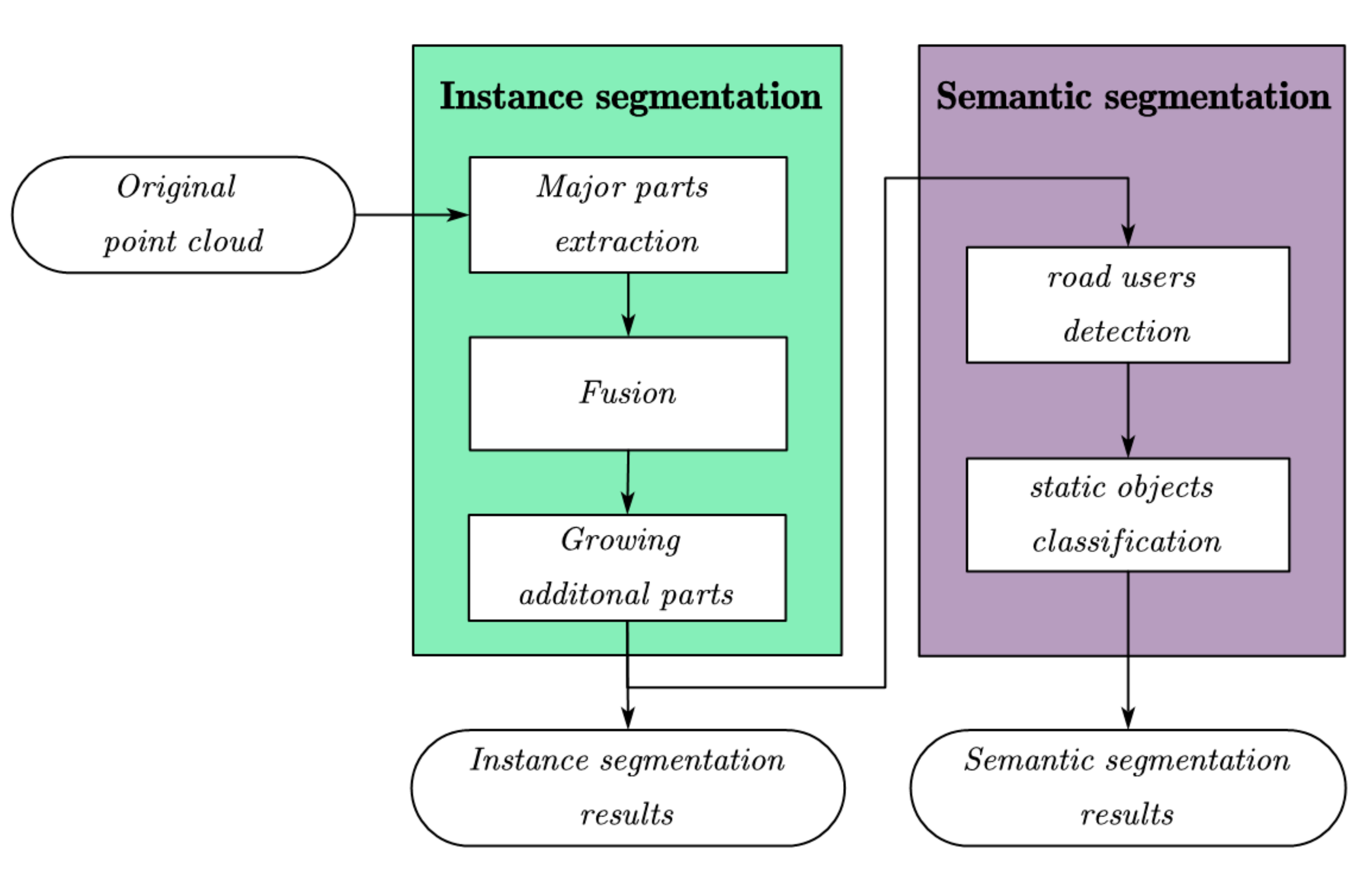
In this paper, the roadside LiDAR point cloud segmentation algorithm is mainly divided into two parts—the instance segmentation part and the semantic segmentation part. The flow chart is shown in Figure 1. Among them, semantic segmentation is based on instance segmentation. We divided all objects into road users (pedestrians and vehicles), poles, buildings, and plants to realize the semantic segmentation of a raw point cloud after instance segmentation.
The main work of this paper includes:
- A novel slice-based segmentation method is proposed. The slice is used as the basic unit to segment the point cloud, which can achieve instance and semantic segmentation of low-channel LiDAR point cloud data.
- For instance segmentation, we proposed a novel regional growth method. Furthermore, to improve the extraction effect in traffic scene instance segmentation, the extraction method of the major part of the object is optimized to solve the occlusion of the traffic objects within the scene.
- A model based on the Intersection-Over-Union (IoU) method using the intersection over minimum volume (IOMin) of the object to distinguish the moving and stationary objects, and a machine learning model-based recurrent neural network (RNN) was used to learn and classify the moving and static objects, which can extract road users from all objects after instance segmentation.
The rest of the paper is structured as follows: Section 2 describes the definition of slice of LiDAR point cloud. The proposed instance and semantic segmentation methods are introduced in detail in Section 3 and Section 4, respectively. The experiments and case studies are presented in Section 5. Section 6 concludes this article with a summary of contributions and limitations, as well as perspectives on future work.
2. Slice of LiDAR Point Cloud
Slice is the basis of the proposed segmentation method, and it is the concept developed by our prior work [6]. This section just briefly introduces the slice with an aim to give readers a systematic view of our study without making this paper abundant and duplicative.
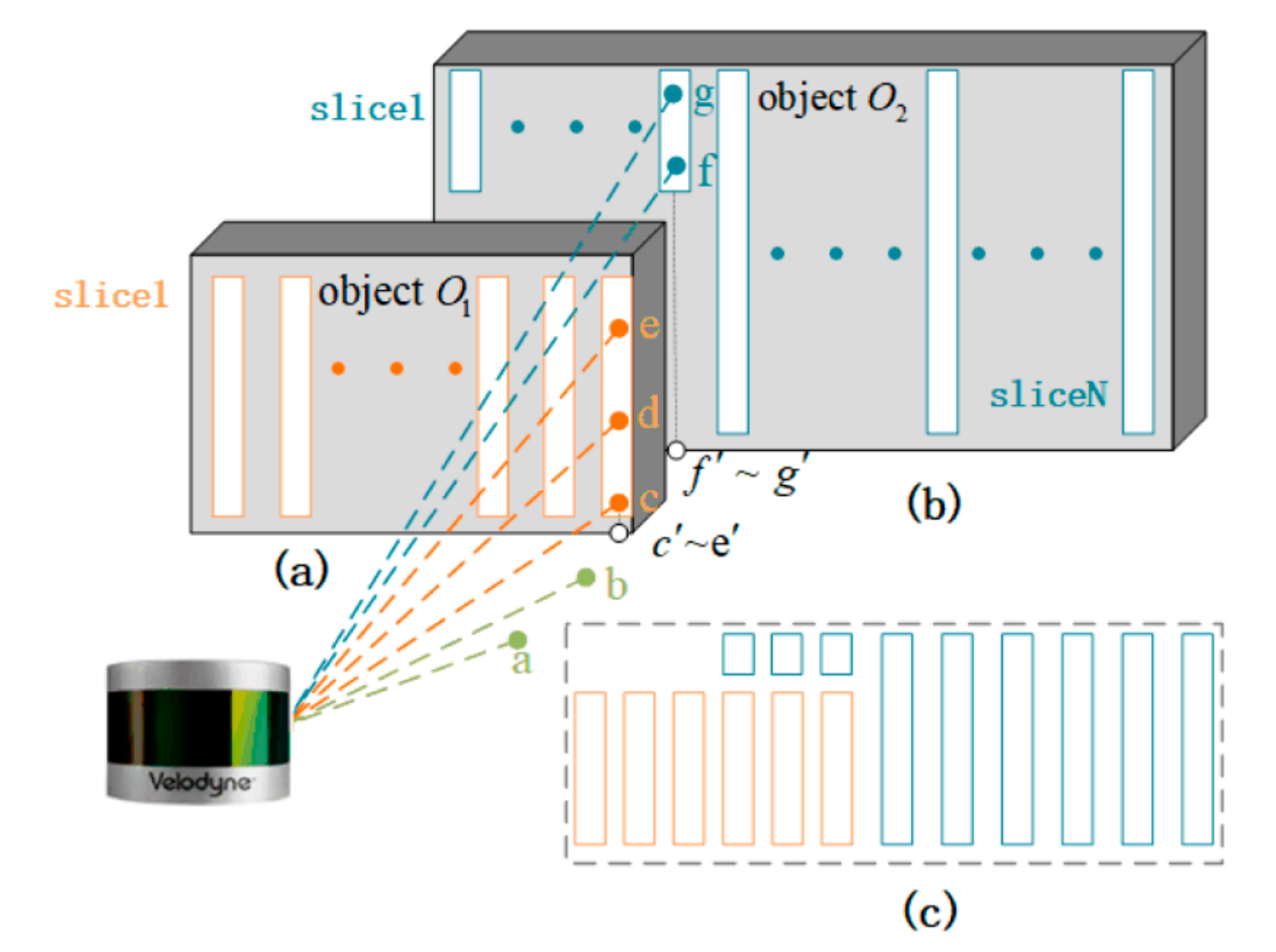
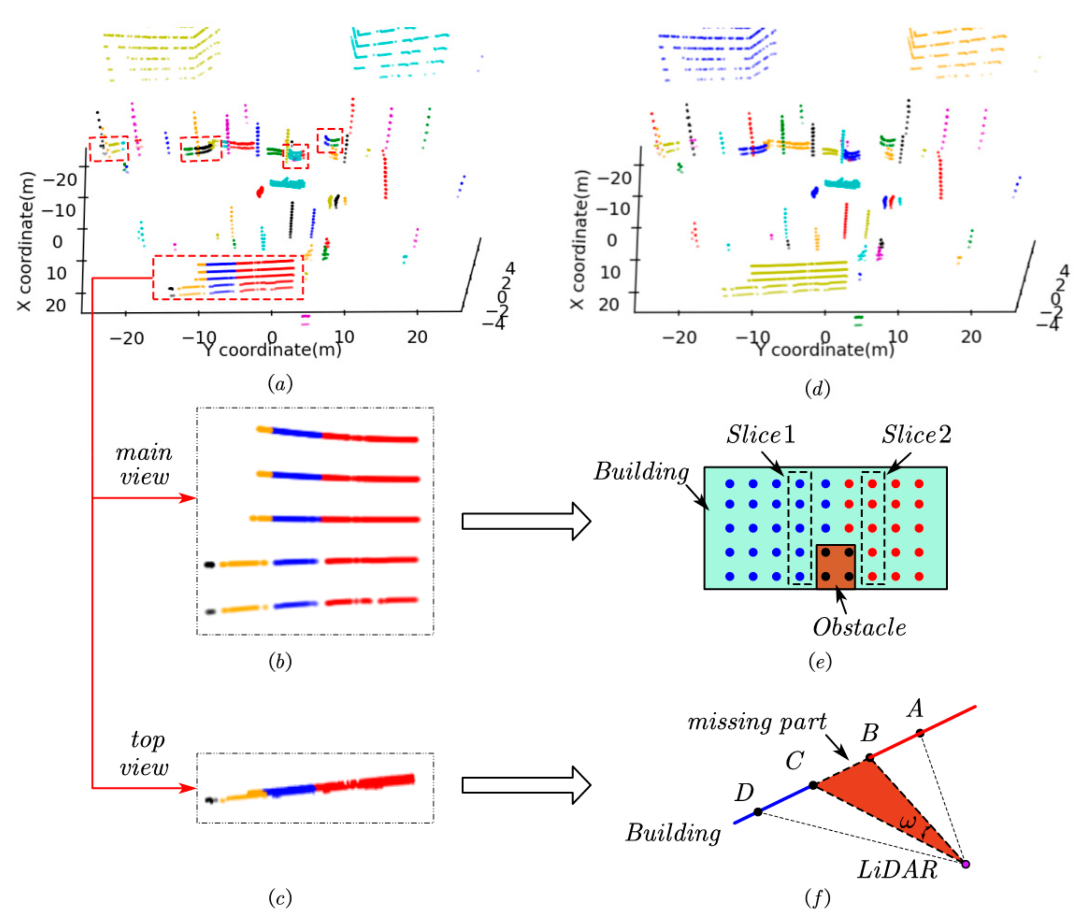
We defined that a slice is a point set containing the points firing on the same object and within the same vertical block. Figure 2 shows the schematic diagram of LiDAR slices, where points a and b are the points firing on the ground by LiDAR; points c, d, e are the points firing on O1, forming a slice of O1; points f, g are the points firing on O2, forming a slice of O2; points c′, d′, e′ and f′, g′ are the points after the projection of points c, d, e and f, g to the horizontal plane, respectively. In fact, a certain object can be represented by several slices in the same vertical plane, as shown in Figure 2a,b. The vertical plane contains all objects’ slices, which are in the same direction, as shown in Figure 2c.
Generally speaking, objects, such as people, vehicles, and buildings, are vertically aligned with the ground. This means that the distance between the points in the same slice after projection is much less than that between different slices. Therefore, we can easily find a distance threshold ∆Rth to abstract all slices in a raw point cloud. All points in a point cloud can be divided into points belonging to a certain slice and a set of single points. In the previous study, we also proposed a highly efficient slice extraction and labeling method. Furthermore, the shape of objects in the real world is not regular so that there may be deviation when we use slices to represent the shape of objects—particularly, at the edges of the object or points of the object is sparse.
Figure 3 shows an example, where Figure 3a shows a raw point cloud and Figure 3b shows all points belonging to the slices when ∆Rth = 0.3 m. Comparing Figure 3a,b we can find that the points belonging to the slices are usually located in the higher density or relatively central area of this object, such as the tree trunk and human trunk, which we call the major part of object. The points that belong to this object but belong to the set of single points are generally located on the boundary of an object or lower density region, such as leaves and human arms, which we call the additional parts. Clearly, the main part of an object has shape stability, while the additional part is variable. For example, when walking, the arm swings, but the human trunk can be seen to remain unchanged. In addition, in windy conditions, the shape of the tree trunk can be seen to remain static, but the leaves are swaying. We can combine the main part and the additional part to represent the object accurately.
3. Instance Segmentation
In this section, we will describe the specific content of an instance segmentation algorithm, named the Slice Growing (SG) algorithm, which is also a region-based method. In this algorithm, the major part of each instance object can be equivalent to seed points in other region-based methods. Therefore, the major parts will be found first, and then, the additional parts will be checked and assigned by the way of regional growth, to finish the instance segmentation of a raw point cloud.
3.1. Extracting Major Parts of Objects
3.1.1. Basic Principles of Extraction
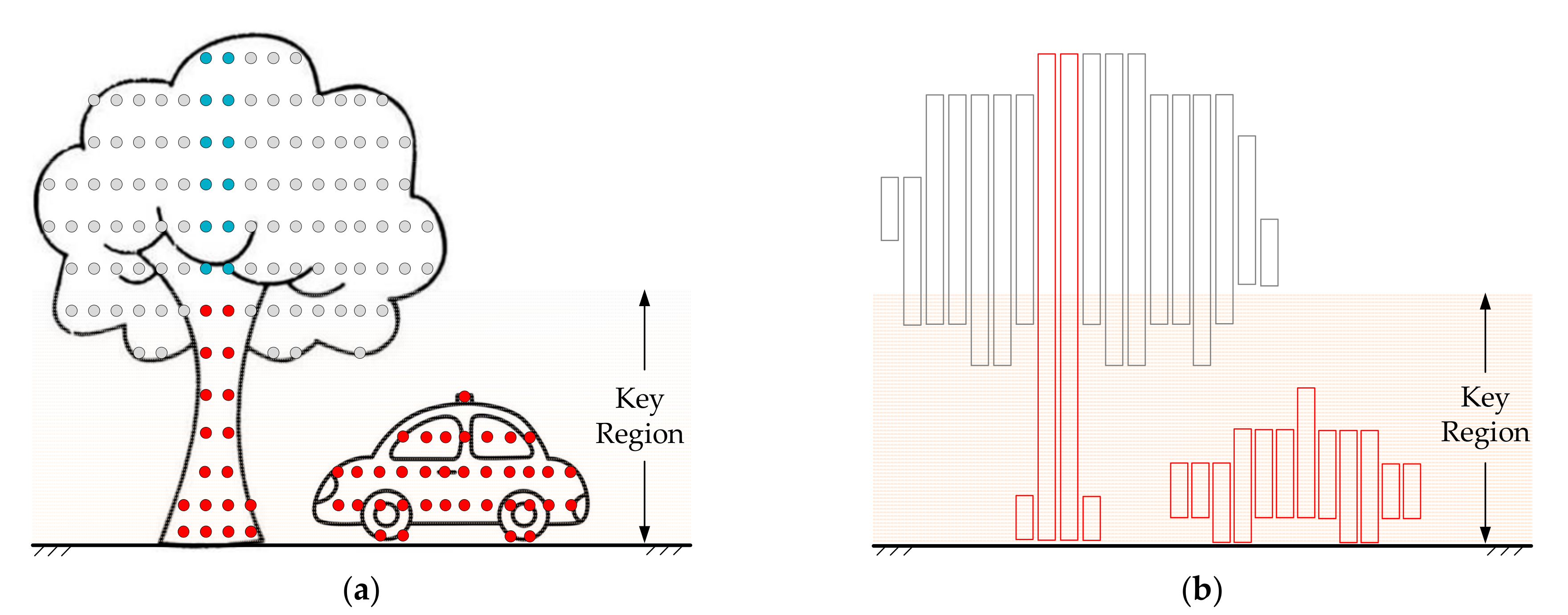
From Figure 3a, it can be seen that a raw point cloud contains a lot of objects, such as road users, roads, and plants. Trees are the most special because the distance between its major part (trunk) and the additional part (leaves) can be very far, and the area covered by the additional part is higher than that of the major part. However, no matter moving road users or the fixed tree trunks, their major parts are all close or connected to the ground, which is different from the leaves. Therefore, a height Hmp can be set to find the major part of the object and exclude the leaves as much as possible. We call the area between the ground and height Hmp as the key region.
For different objects in the traffic scene, the height Hmp is different, thus the height of the major parts is also different. Therefore, it is impossible to find a Hmp to ensure that all points of the major parts are within the range but all points of additional parts are out of the range. However, it just needs to find out the major part points of the object in the key region. Within the same slice, the major part points out of the key regions belong to the same object. Figure 4 is the schematic diagram of this process. Figure 4a shows the schematic point cloud of a tree and car scanned by a LiDAR sensor, where the red points belong to major parts within Hmp, blue points belong to major parts but above Hmp, and gray points belong to the additional parts. It is obvious that the blue points and the red points in the same vertical block belong to the same slice, as shown in Figure 4b. Based on Figure 4a,b, all points of the major part could be found.
3.1.2. Implementation and Limitations
In this paper, road users (vehicles, pedestrians) are the main target objects of HRMTD that the LiDAR sensor wants to collect. Therefore, we should set Hmp slightly lower than the general height of road users, to ensure that most of the major parts can be included, and most of the roadside leaves can be excluded. In China, the average height of male adults is about 1.71 m, and it is about 1.6m for female adults [32]. The height of small cars is generally between 1.6 and 1.8 m. Therefore, we set Hmp to 1.5 m in this paper. In this height range, there are a large number of points belonging to major parts and a small number of points belonging to additional parts. Moreover, the points within the major parts are denser than those within the additional parts. If projecting all points in this range to the ground, it will find out that the point density in the major part is denser, and sparser in the additional parts.
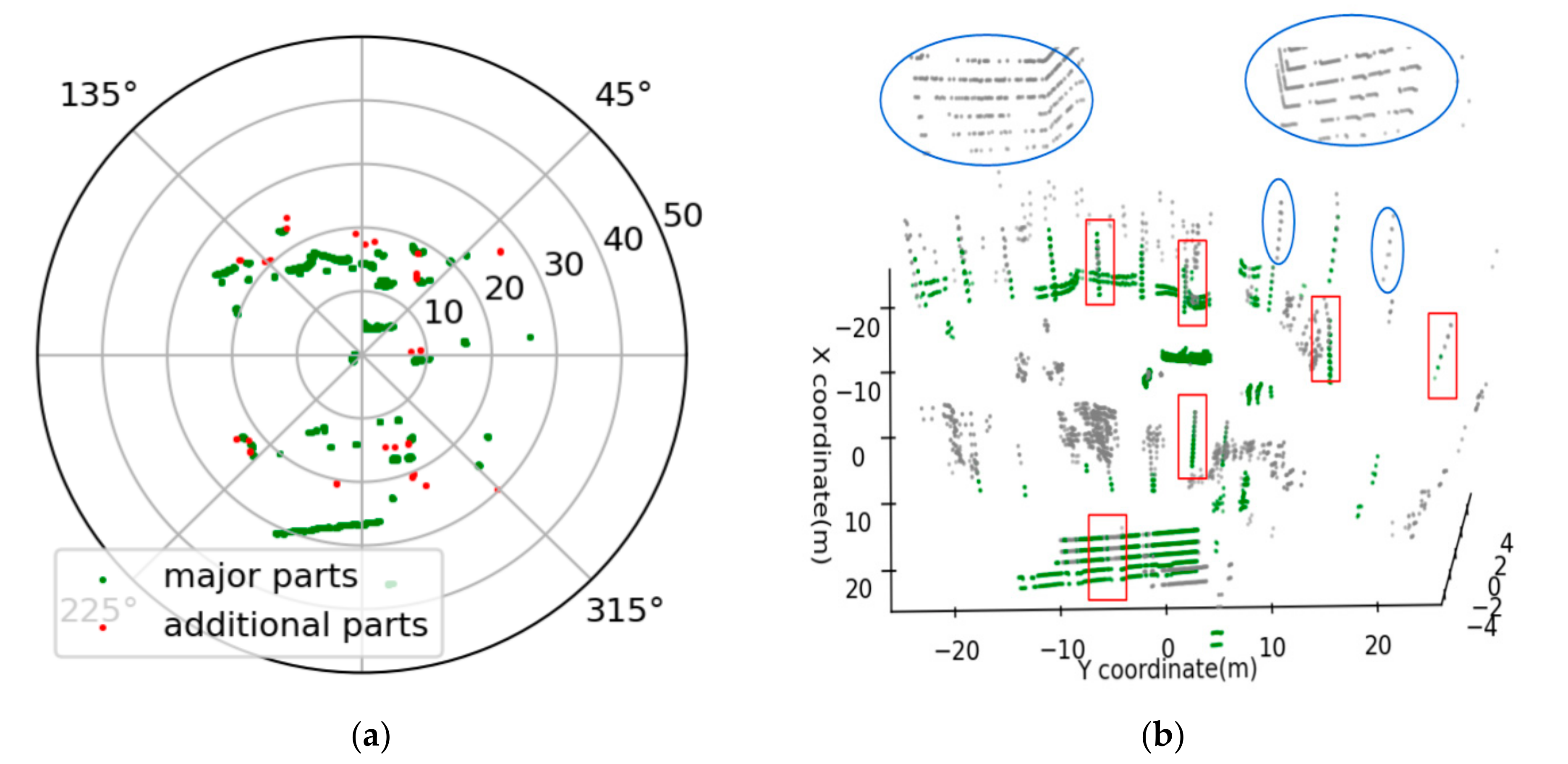
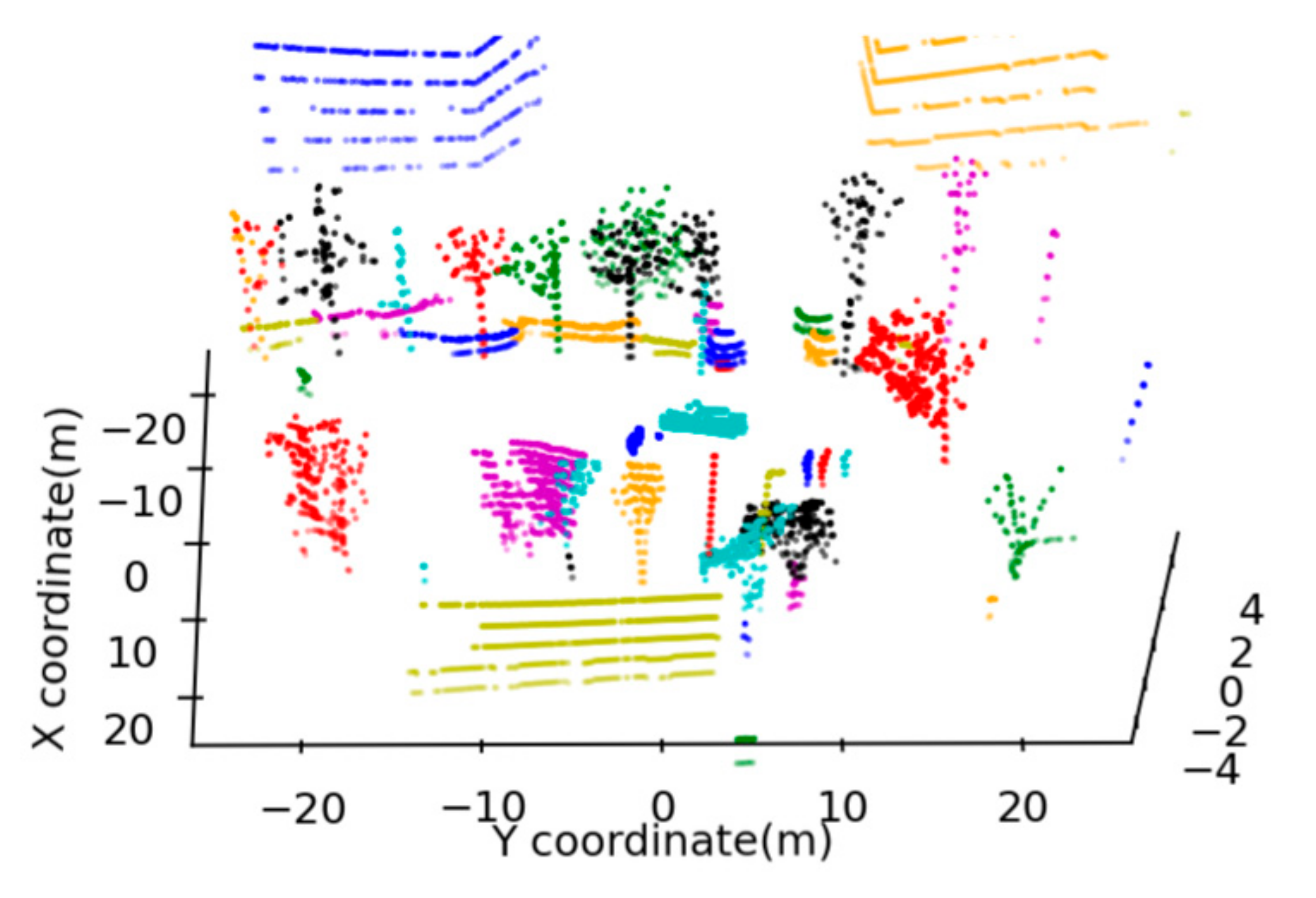
Based on this phenomenon, the Density-Based Spatial Clustering of Applications with Noise (DBSCAN) [33] algorithm can be used to extract the major part of objects. DBSCAN is a density clustering algorithm with two important parameters: minimum number of points (MinPts) and epsilon (ε). One object will be joined in the clustering area if its point density is higher than or equals to a pre-defined MinPts and its distance to the center is less than a pre-defined ε. In our experiment, we set MinPts = 3 and ε = 0.008 m to cluster the projected points in the key region of the point cloud shown in Figure 3a. Figure 5a shows the results of DBSCAN clustering, where the green scatters are denser points that belong to the major part and the red scatters are sparser points that belong to the additional parts. Figure 5b is the corresponding 3D display, where the green scatters are the major parts found by clustering, and the gray scatters are all slices of the input point cloud. Comparing Figure 3, we can find that some major parts were not found accurately. This can be summarized into the following two types of errors:
- The major part is incomplete (Error 1). The reason for this kind of error is that the major part of the objects in the real world is not always regular or vertical to the ground, which will lead to the major part points of the object in the non-key region and the major part points of the object in the key region not belonging to the same slice. This phenomenon will result in not being able to detect the incomplete major part in the non-key region. The red rectangles in Figure 5a are typical examples.
- The major part is missing (Error 2). The reason for this problem is the occlusion. Due to the characteristics of the LiDAR sensor scanning, the scanning objects far away from the LiDAR sensor are easily obscured by the near objects within the scanning range. The absence of the major parts occurs when the major part of the object in the key region is occluded by another object. The blue ellipses in Figure 5b are typical examples.
3.1.3. Improvement
Comparing the slices with the major part of different objects, the distance of slices within the same object is closer than the distance between the different objects. Therefore, we can set a threshold distance Dth to distinguish which slices belong to each object with the incomplete major parts, as to solve Error 1. That is,
where S is a slice; M is a major part;
is the distance between S and M. The slice and major part are both sets of points. Thus,
is equal to the minimum distance between the points in S and the points in M, which is
where
is the 3D distances between points Pi and Pj.
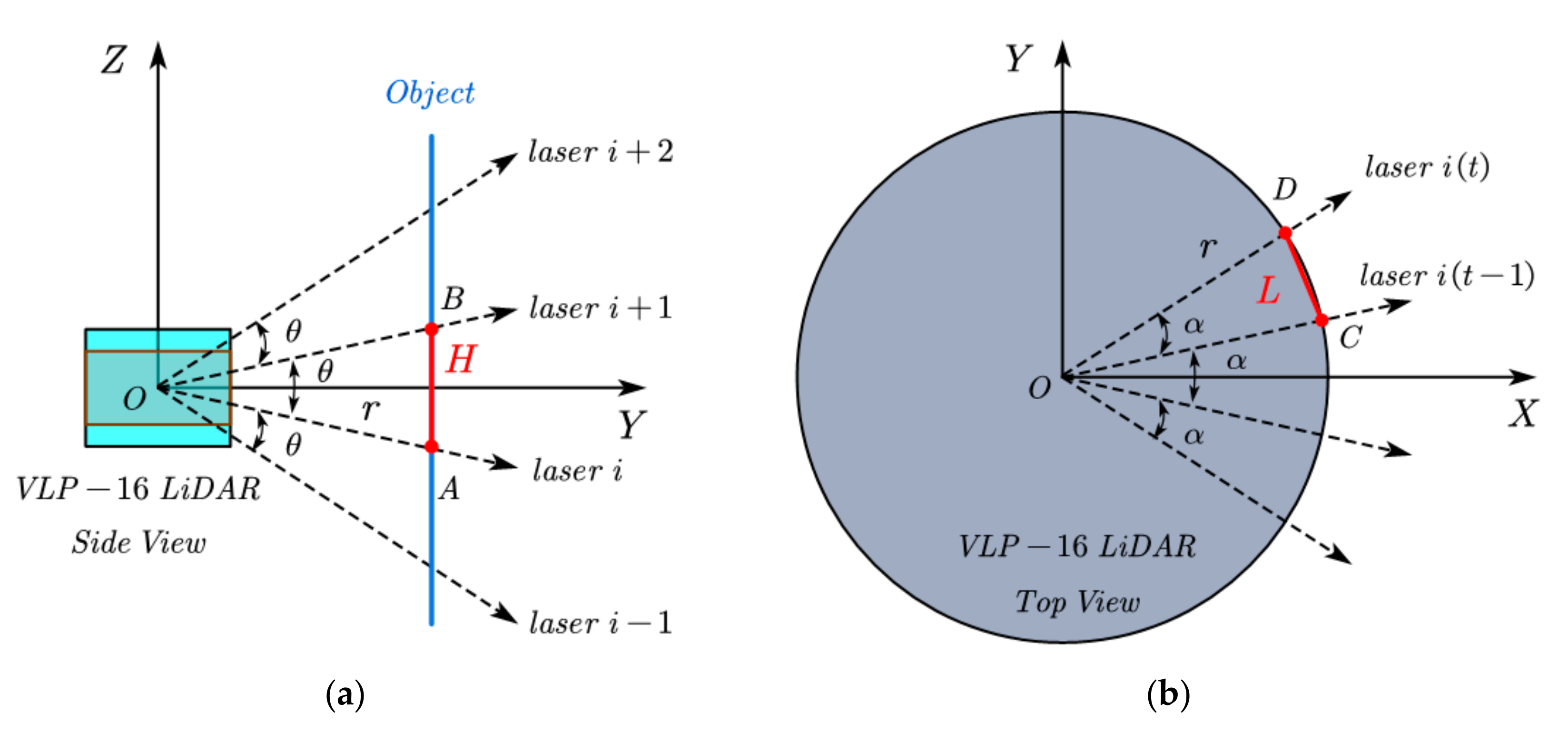
The working principle of LiDAR is to obtain the distance information of objects by firing and receiving laser beams, and it outputs polar coordinate data. Figure 6a,b are the schematic diagrams for calculating the distance between two adjacent points of the LiDAR in the vertical and horizontal directions, respectively. Then,
where H is the vertical height between two adjacent points at the same distance r; r is the 2D distance between the data point and the LiDAR sensor; L is the horizontal distance between two adjacent points collected by the same laser beam; θ is the vertical angular resolution of the LiDAR sensor (For VLP-16, θ = 2°); α is the horizontal angular resolution of the LiDAR sensor (α = 0.2° is set in this paper).
From Equations (3) and (4), it can be deduced that the value of H and L increases as the distance from the LiDAR sensor to the object increases.
If two slices are adjacent, the maximum distance Dmax between the two slices is
At this time, the difference between the vertical angle and the horizontal angle of the two nearest points in the two slices is θ and α, respectively. Therefore, we can set Dth equal to Dmax to judge which slices around the incomplete major part also belong to this major part, to reduce the impact of Error 1 on the results. In addition, H and L are both related to r. Thus, Dmax is related to r as well. For practical convenience and efficiency, we set r to be the average of all 2D distances between points in the slice and the LiDAR sensor.
To solve Error 2, we need to find the absence of major parts within the gray points in Figure 5b, where the disturbance of leaves is the biggest. Comparing the leaves with major parts, it can be found that there are obvious differences between the two characteristics:
Therefore, the following two steps were used to finish the extraction of major parts in the non-key region:
- Difference 1: the leaves belong to additional parts, and the points in leaves are sparser;
- Difference 2: the average number of points per slice of the leaf is lower than that of the major part. That is because the leaves are relatively sparse and that there are a large number of slices formed by two points.
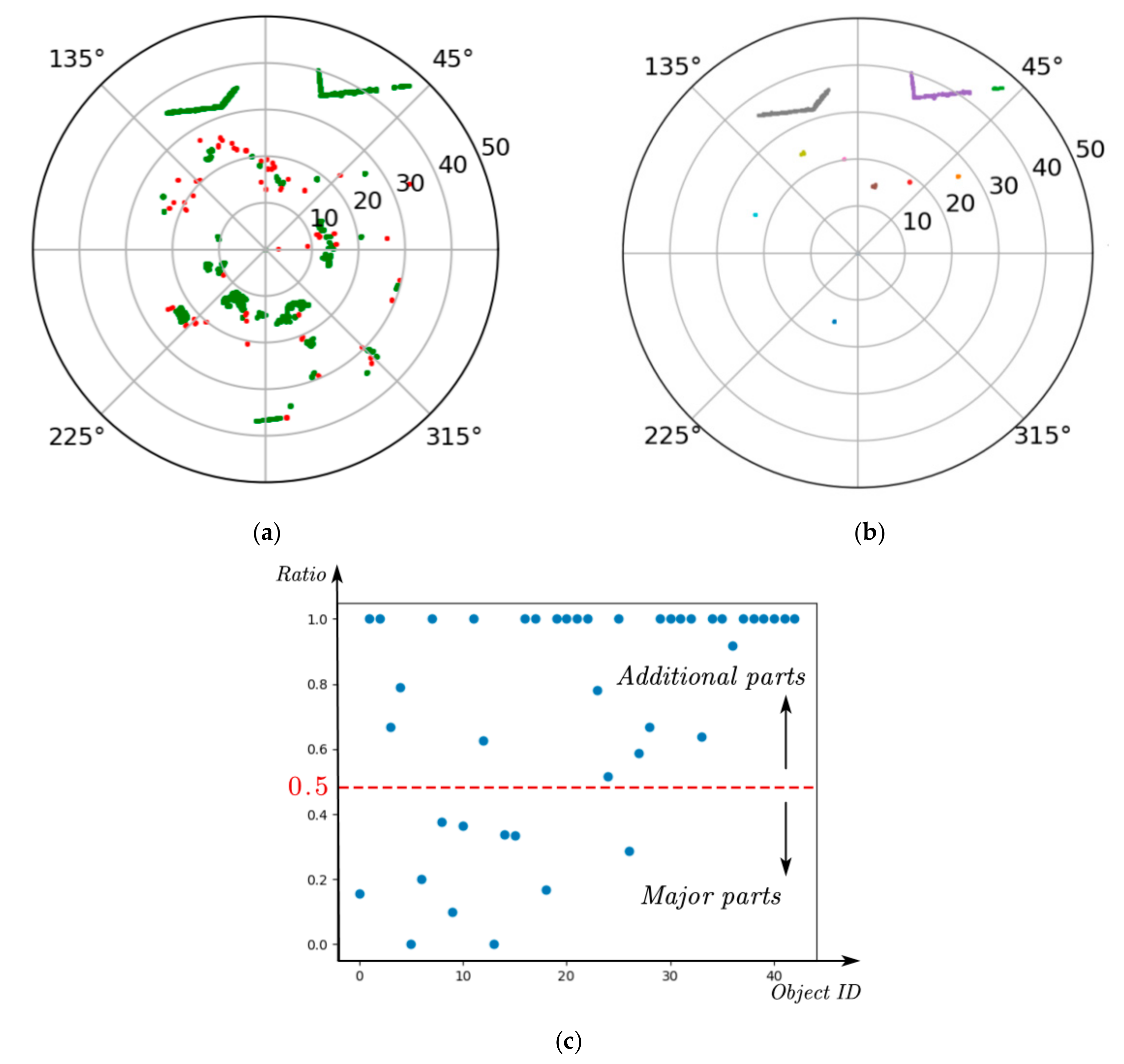
Step 1: Like extracting major parts in the key region, we used DBSCAN to cluster the projected points to obtain high-density points. However, the leaves are more abundant in the 2D plane, which are also considered as high-density points. Figure 7a shows the results, where green scatters are high-density points and red scatters are the exclusive points.
Step 2: Due to Difference 2, we calculated the ratio of slices formed by two points in objects clustered by Step 1, as shown in Figure 7c. It can be seen that a ratio of 50% can well divide these objects into two parts. The objects have a high ratio and 50% belong to the category of additional parts, and the others belong to the major parts. Clearly, if the ratio is high, then some high-density leaves would be identified as major parts.
The results of extracting the major parts in the non-key region are as shown in Figure 7b. The colors in Figure 7b are randomly generated, and different colors represent that the two objects do not belong to the same class.
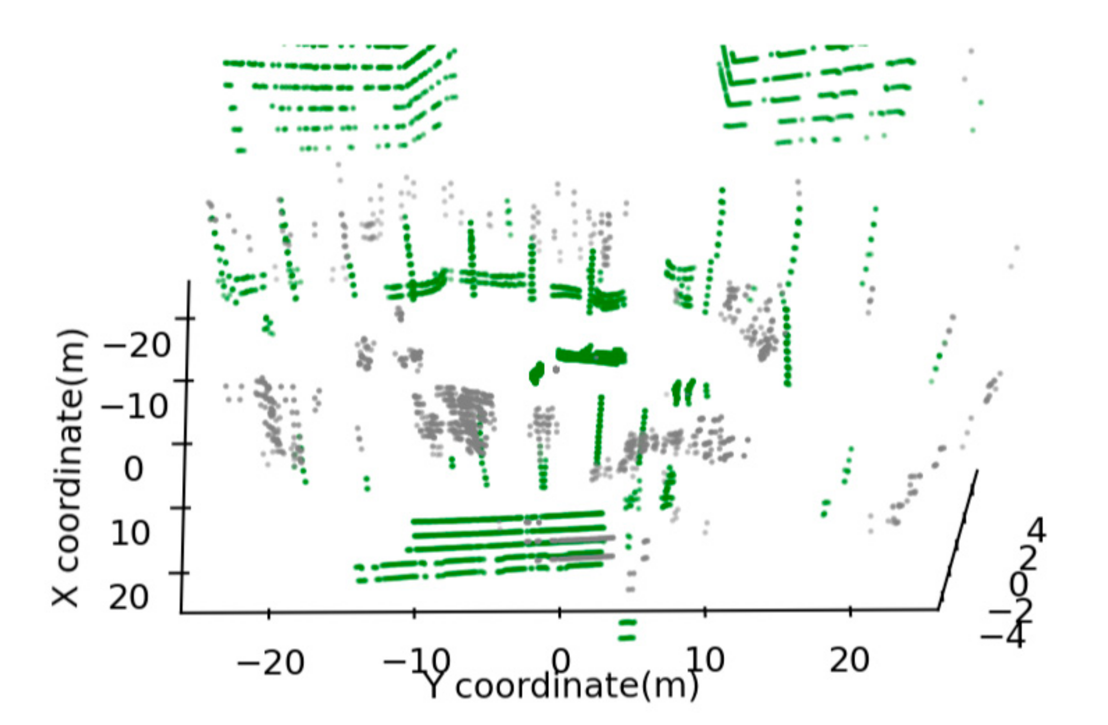
Combining the major parts extracted from the key region and the non-key region, the major parts of all objects can be obtained, as shown in the green scatter in Figure 8. Comparing with Figure 5b, we can find that the accuracy of obtaining the major part has improved by considering Error 1 and Error 2.
3.2. Fusing Major Parts
The DBSCAN was used in extracting major parts from the point cloud. Thus, the points belonging to major parts are not only extracted, but also clustered. Figure 9a shows the result of clustering, where colors are randomly generated, and different colors mean different classes (objects). However, we can see that the major parts of an object may be clustered into multiple parts. The major parts in the red dashed box in Figure 9a are examples. Thus, we should fuse those major parts.
Figure 9b,c show the top main view and the top view of the building in the bottom of Figure 9a, respectively. The main part of this building is divided into four parts due to the occlusion of the objects in front of it. In this paper, we only consider a small part of the occlusion. Otherwise, too much information will be lost for the occluded objects. Figure 9e is a schematic diagram of the main view of the obscured building, where the building is divided by the obstacle into two parts—the blue part and the red part. Moreover, those parts should belong to the same object. Therefore, the nearest two complete slices, such as slice 1 and slice 2 in Figure 9e, are similar to each other. We use the number of points in a slice to measure the similarity between the two adjacent slices, then,
where n1 and n2 is the number of points in slice 1 and slice 2, respectively; ∆n is the difference which can measure the similarity of two slices; N is a threshold of the similarity. In general, if the same kinds of objects have the same height and same distance from the LiDAR sensor, the point number in the slice of the objects would be equal. In this paper, we set N = 1. That is, if the adjacent slices have the same point number, and they have the same height and the same distance from the LiDAR sensor, then the adjacent slices belong to the same object.
It can be seen from Figure 9c that only the side of the object close to the LiDAR can be detected. All slices of an object are projected to the ground, which can be fitted by a curve line. If just a small part of the object is selected, the projection of the slice can be fitted with a straight line by using the least square method. When only a small part is covered, the change trend of the position of the slices adjacent to the missing part should be similar, as shown in Figure 9f. Then,
where kXY is the slope of the line from X to Y; ∆k is the maximum slope difference between the missing part and its adjacent parts after fitting; K is the threshold of the change trend.
It can be deduced from Equation (7) that the value of K is a negative correlation with the flat of the object.
This paper sets K = 0.15. In the experiments, if the value of K is set too large, adjacent objects may be recognized as one object. For instance, two pedestrians are walking together. If K is set too small, even if only a small part of an object is blocked, this object with an uneven surface may be recognized as two objects.
The missing part is the small part of an object. Therefore, the shortest distance between the two ends of the missing part (such as the length of segment BC in Figure 9f will not be too long and there will be a limit. According to Equation (4), with the same horizontal angle ω, the farther the object from the LiDAR, the larger the missing part will occur. Therefore, this limit should change with the distance of the object. Then,
where ∆d is the shortest distance between the two ends of the missing part; r is the average of all 2D distances between points in the slices of major part and LiDAR; D is a constant, and the smaller the value, the larger the range of occlusion allowed. This paper sets D = 20. In the experiments, if the value of D is set too small, the objects with the same classification which are far away from the LiDAR sensor would be recognized as one object, such as adjacent trunks with the same height. If D is set too large, the object will be divided into two different objects even if there is just a small occlusion.
If Equations (6) to (8) are satisfied, it can assume that the two major parts belong to one object. The results of the major part fusing operation are shown in Figure 9b. Although this theory is relatively simple, it can achieve better results in the experiments.
3.3. Growing
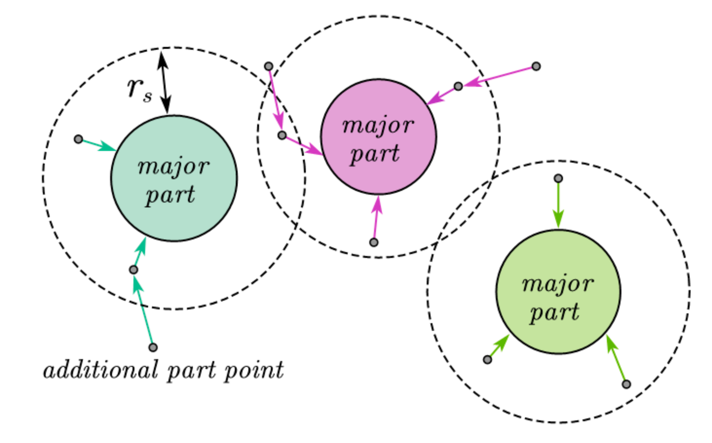
After extracting the major part of the object, the remaining points in the point cloud are single points mostly. These points belong to the additional parts of the object or the ground points. In our previous work [6], we proposed a slice-based ground point segmentation method. After removing the ground points, the points of the additional parts can determine which major part it belongs to according to the distance, as to finish the instance segmentation of a whole point cloud. Generally, for an object, the points of its additional part are scattered around its major part. Thus, we can take the major part as the center and the radius as rs to search for its additional part points from near to far. When a point is in the search range of multiple major parts, it belongs to the nearest major part. The schematic diagram of the growing points of additional parts is as shown in Figure 10.
For VLP-16, the horizontal angular resolution of LiDAR is higher than the vertical angular resolution. Therefore, at the same distance, the adjacent two points in the vertical direction are more than those in the horizontal direction. To ensure a normal growth process, rs should be greater than the shortest distance between two adjacent points in the vertical direction. As can be seen from Figure 7a, the 2D distance of most of objects in the point cloud is generally less than 30 m. In addition, at 30 m distance, the vertical height between two adjacent points is:
. Therefore, this paper sets rs = 1 m. After growing, the instance segmentation process is completed, and the results are shown in Figure 11.
4. Semantic Segmentation
In instance segmentation, all points belonging to an object have been found. Further classifying and labeling the objects in the point cloud will achieve the effect of semantic segmentation. This section will illustrate a method to classify and label the objects in the point cloud into four categories: road users, poles, buildings, and plants.
In the traffic scene, the road users are mobile and can appear anywhere in the detection range of the point cloud theoretically. At the same time, the other objects such as poles, buildings, and plants are relatively fixed. As the detecting object is always far from the LiDAR sensor, less information can be obtained [9]. Especially for low-channel LiDAR, using a frame of a point cloud cannot even distinguish pedestrians and stones of the same height in the distance. Therefore, in this paper, the objects in the point cloud are divided into two steps for semantic labeling. Firstly, the moving road users in the point cloud are labeled by using the timing information of the multi-frame point cloud, and then, the remaining static objects are labeled.
4.1. Labeling Moving Objects
Axis-aligned bounding box (AABB) is the most commonly used method to represent a 3D object. It is a rectangular box with six surfaces which normally parallel with the standard axis. As mentioned above, the major part of an object is relatively fixed, while the additional part is relatively variable. For example, when the wind blows, the leaves swing against the wind, while the trunk is relatively fixed. If we use an AABB formed by all points to represent this object, even if the object is static, the bounding box may change greatly. Therefore, to distinguish moving and fixed objects stably, this paper uses the AABB formed by the major part to represent a certain object, as shown in Figure 12.
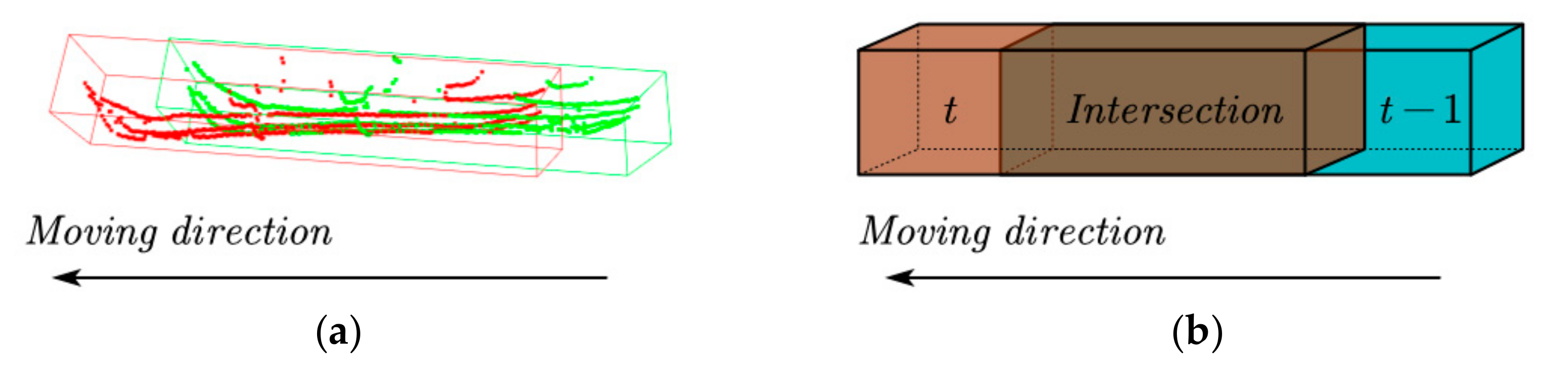
It takes a short time for the LiDAR to rotate around (0.1s for VLP-16). Therefore, no matter moving or static objects, there will be an intersection between the two frames of point clouds. As shown in Figure 13a, the red point is the car detected in the current frame of the point cloud, and the green point is the car in the point cloud of the previous frame. Figure 13b is a schematic diagram of this process using AABB.
For a static object, the intersection will be close to the volume of the object; for a moving object, the intersection will be much smaller than the volume of the object. Therefore, the intersection can be used to distinguish between moving and stationary objects. We used intersection over minimum volume (IOMin) to measure and show the intersection, as shown in Equation (9):
where Vt is the volume of an object in the point cloud at frame t; Vt−1 is the volume at the last frame; Vt∩Vt−1 is the volume of the intersection of Vt and Vt−1.
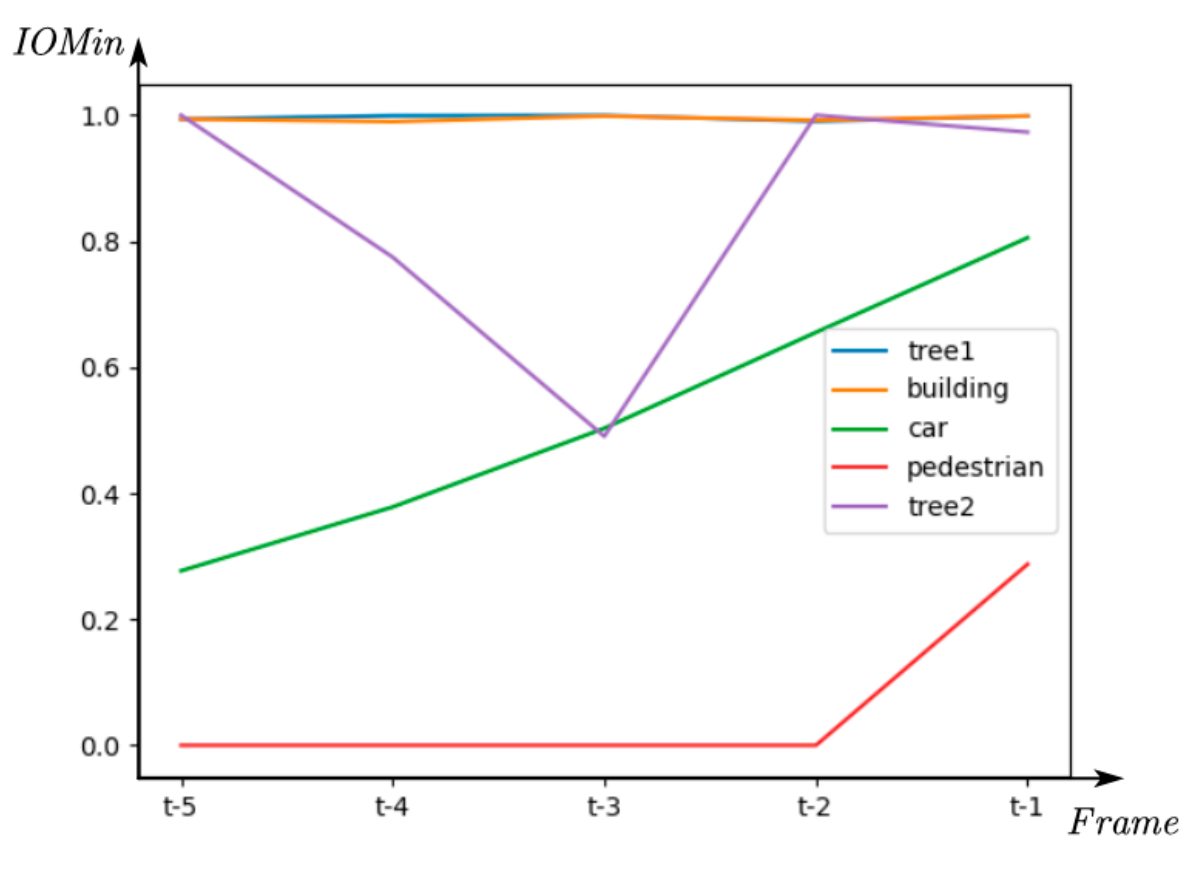
We calculate the IOMin of different objects in the current frame and the first five frames, respectively, as shown in Figure 14. It can be seen that different objects can obtain different types of curves. For static objects (trees and buildings), the IOMins are usually close to 1 no matter what frame it is, such as tree1 and building in Figure 14. For moving objects, the further away they are from the current frame, the smaller the IOMin. This is due to the movement of objects. The curves of cars and pedestrians in Figure 14 are also different, which is caused by their different shapes. Occlusion in the point cloud is inevitable, which will also affect IOMin. At the t − 4 and t − 3 frames of tree2 in Figure 14, IOMin decreases to a certain extent because the trunk of tree2 is partially covered by moving objects.
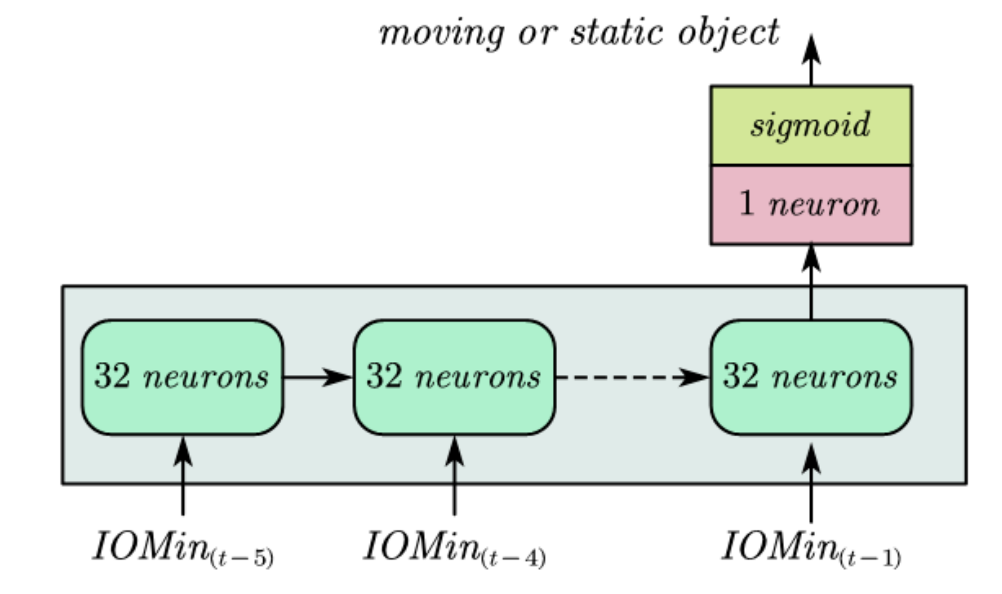
To find moving objects from the IOMin sequence, a machine learning model-based recurrent neural network (RNN) [34] was developed, as shown in Figure 15.
In Figure 5, the IOMin sequences are the input cells. Each cell contains 32 neurons whose activation function is ReLU. The proposed method only distinguishes moving and static objects. Therefore, only one neuron connected with the output in the last step, and the activation function is set as a sigmoid function. The timing information of moving objects can be transferred between the recurrent cells. In the model training period, the optimizer was Adam, and the batch size was set as 16. We called this RNN model “IOMin-RNN”.
In the experiments, we found that the ratio of positive (moving object) and negative (static object) samples is not balanced after making about 5500 frames of LiDAR data. The positive sample is 1/9 of the negative sample. Therefore, if the cross entropy is used as the loss function, then the loss function will bias to the side with more samples during the training, which will make the loss function very small, but the classification accuracy is not high for small samples. Thus, we give different weights to positive and negative samples to balance the loss of each class. The loss function is defined as follows:
where X is the input of samples; y is the category of the output; WN is the weight of negative samples; WP is the weight of positive samples;
is the loss of positive samples;
is the loss of negative samples; Ntotal is the total number of samples; NN is the number of negative samples; NP is the number of positive samples.
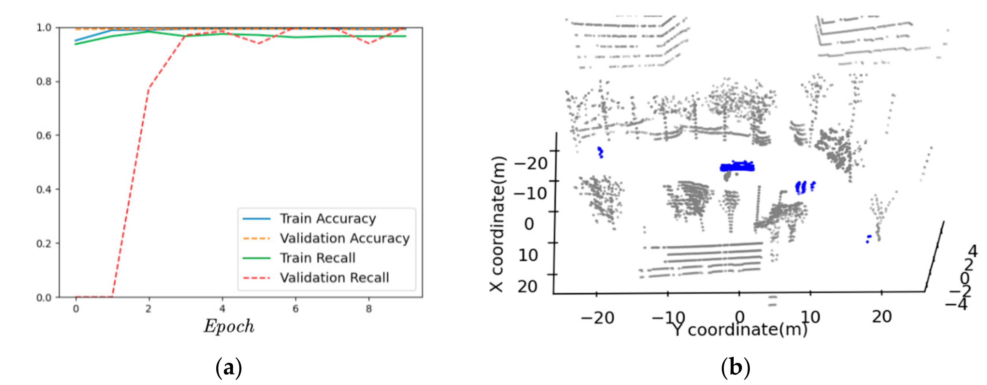
To overcome the overfitting issue, 80% of the datasets were used to train and 20% of the datasets were used to validate. After 10 epochs, the accuracy of road user identification can be up to 98.7% and the recall can be up to 99.9%, as shown in Figure 16a. Figure 16b shows the results of labeling road users.
4.2. Labeling Static Objects
After excluding the moving objects in the point cloud, attention can now be directed to the classification of different static objects, including buildings, poles, and plants. For this purpose, three features were extracted from the static objects:
- Feature 1: the ratio of major part points to all points. The calculation equation is shown as Equation (11):where M is the point number contained in the major part of an object; N is the point number contained in this object.
- Feature 2: volume of the major part. The calculation equation is shown as Equation (12):where H is the height of the AABB of an object; W is the width of the AABB of the object; L is the length of the object.
- Feature 3: the height of the major part divided by the width. The calculation equation is shown as Equation (13):where H is the height of the AABB of the major part of an object; W is the width of the AABB of the major part of the object.
The points of the major part of an object are relatively fixed, so the above three features are based on the major part features.
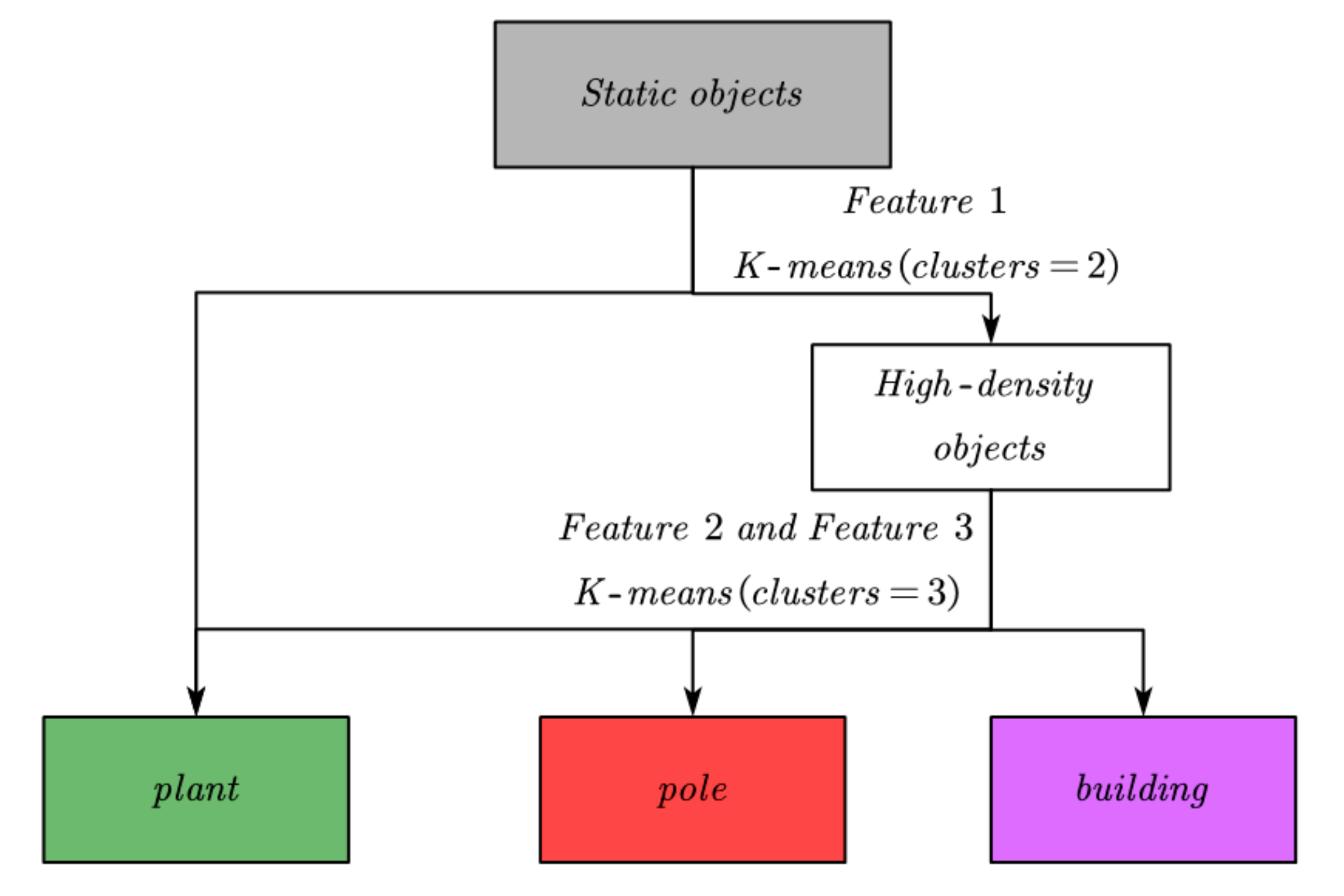
If a tree has a large number of leaves, the value of Feature 1 will be smaller, while other static objects will be larger. Therefore, we can use Feature 1 to divide the objects in the point cloud into sparse and high-density objects. The sparse objects belong to plants, and the high-density objects include buildings, poles, and a small number of short and leafy shrubs. Buildings are usually far away from LiDAR and are very large. The poles are thin and long. Therefore, combined with Feature 2 and Feature 3, high-density objects can be reasonably divided into three categories, in which the objects whose volume is very large belong to the building, the objects whose height divided by the width is very large belong to the pole, and the remaining objects belong to the plant. To sum up, the process of labeling static objects is shown in Figure 17.
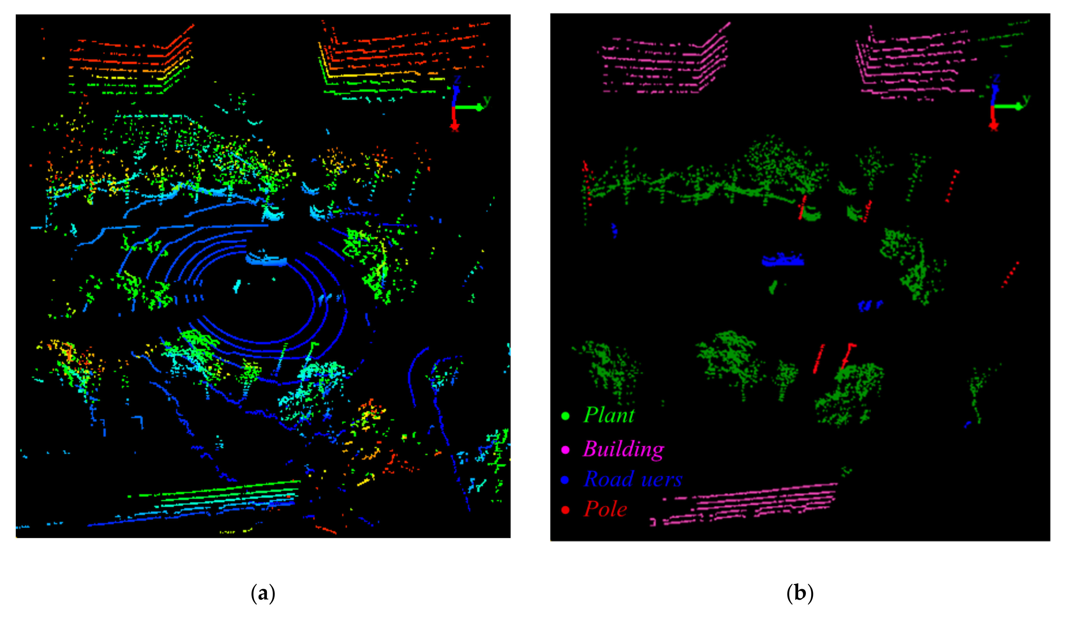
After labeling moving objects and static objects, we have completed the semantic segmentation of all objects in the point cloud, and the results are shown in Figure 18. This paper does not separate pedestrians and cars from road users. This is because it is difficult to obtain good results only by moving the characteristics of objects. In future work, we will separate them from other features, such as point number and shape of each road user.
5. Experiment
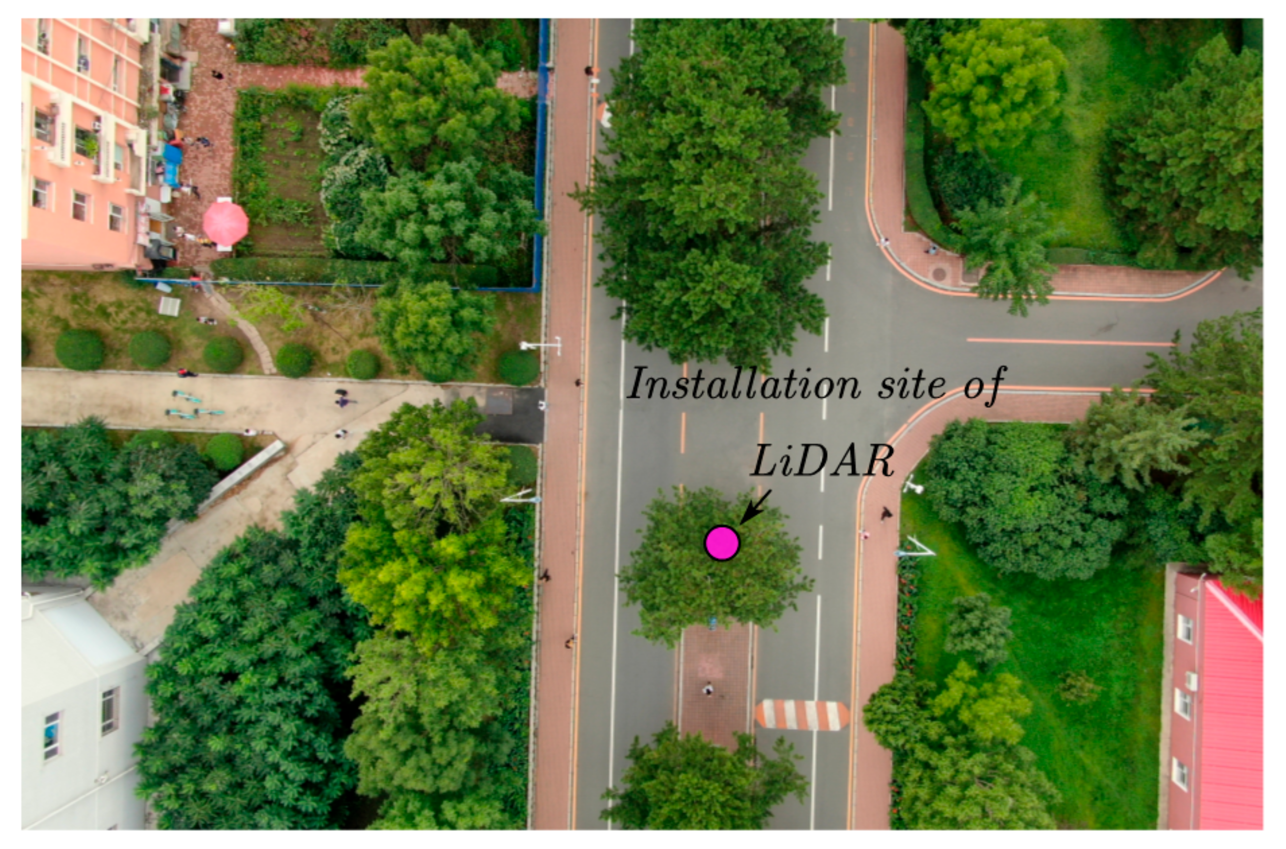
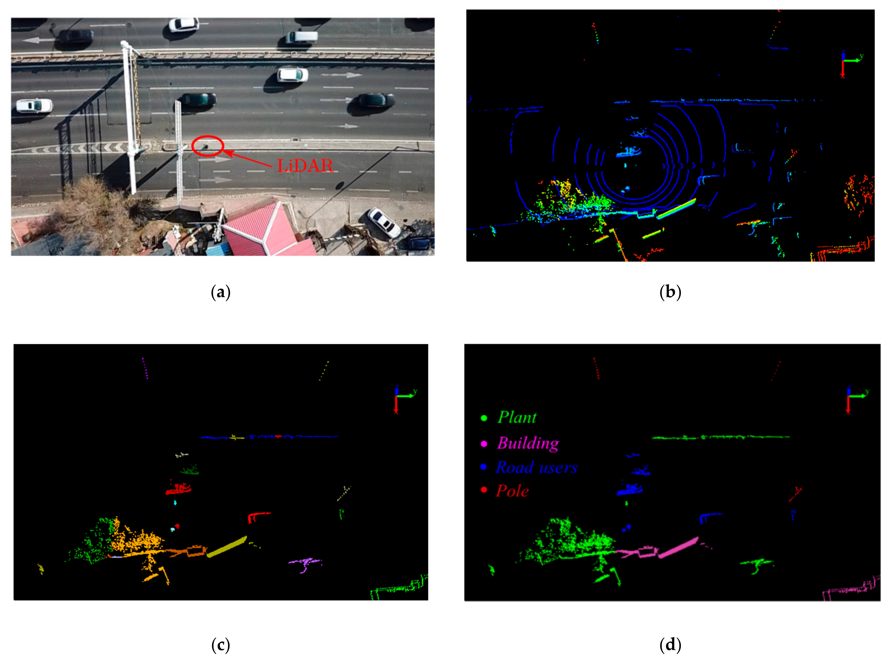
The data used in this work were obtained from a previous study on the background point filtering of low-channel infrastructure-based LiDAR data [6]: we collected approximately 1200 frames of point cloud data by the Velodyne VLP-16 LiDAR sensor at Central Avenue, Nanling campus, Jilin University. The location (Location 1) of the LiDAR sensor is latitude 43.85° N, longitude 125.33° W. An aerial photograph of the corresponding location is shown in Figure 19. In the experiments, the detection range of the LiDAR is 100 m, the vertical angular resolution of the LiDAR sensor is 2°, the horizontal angular resolution of the LiDAR sensor is 0.2°, and the rotational speed is 10 rotations per second.
5.1. Instance Segmentation Evaluation
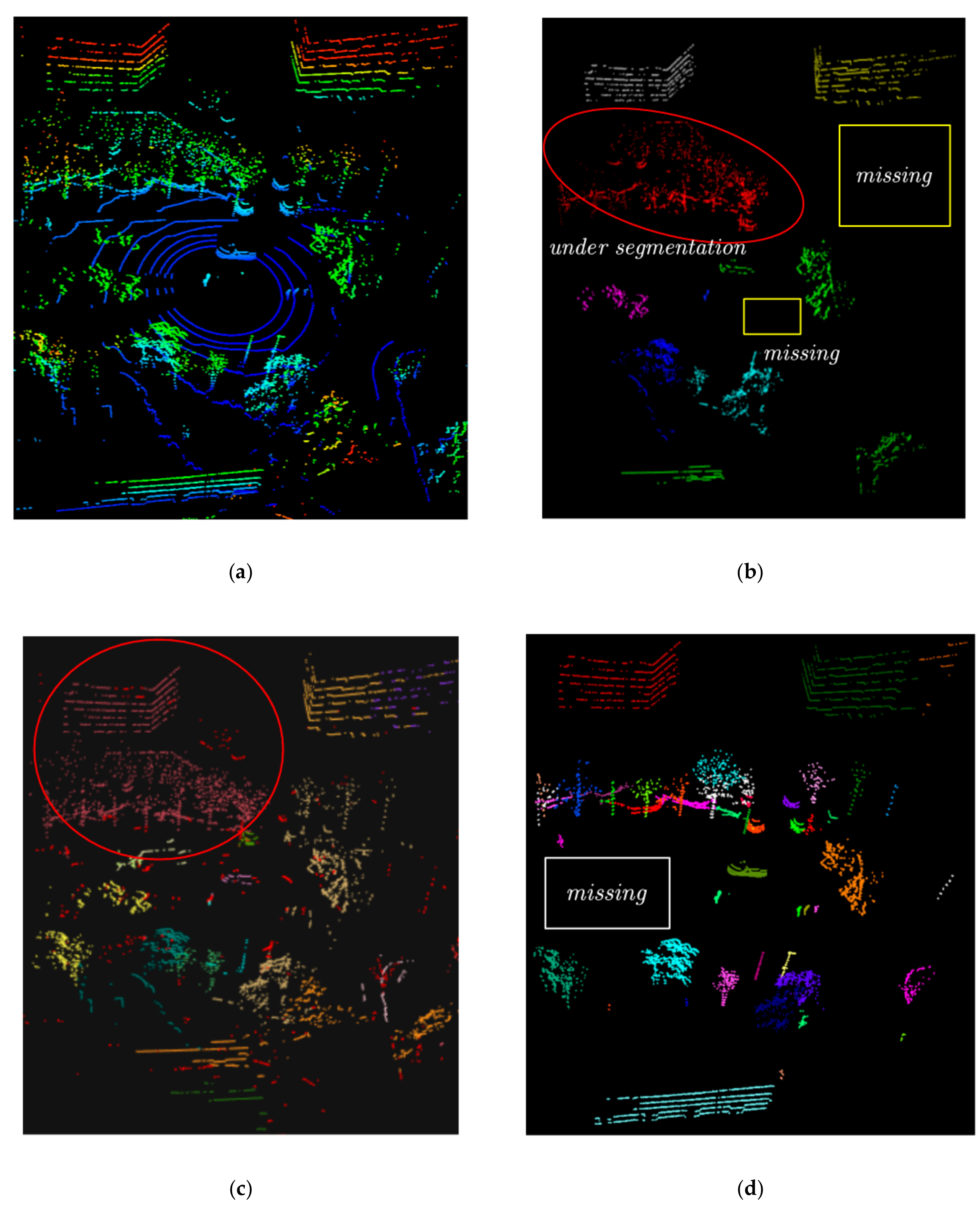
To evaluate the instance segmentation algorithm described in Section 3, we compared it to a Euclidean-based segmentation algorithm [35] and the regional growth algorithm in Point Cloud Library (PCL) [36]. For Euclidean-based segmentation, we set the search radius of the cluster to 1m, set the minimum number of points required for a cluster to 10, and set the search mode to KD-Tree. Figure 20b shows the results of the Euclidean-based segmentation algorithm. For the regional growth algorithm in PCL, the selection of seed points is based on normal and curvature, the growth process is compared by the curvature and normal of the seed and its surrounding adjacent points. We set the threshold of curvature to 1 m−1 and the threshold of normal to . Figure 20c shows the results of the regional growth segmentation algorithm in PCL.
Figure 20d shows the results of the proposed algorithm. By comparison, it can be found that the proposed algorithm can reasonably segment the point cloud. While the Euclidean-based segmentation algorithm and the regional growth algorithm segment multiple objects into one object (under segmentation), the objects within the red ellipse region are examples. The density of the low-channel LiDAR point cloud is lower. There, in the open environment, the Euclidean-based segmentation algorithm will cause a small volume object to go missing, as shown in the yellow box in Figure 20b.
We also count the actual number of objects in the original point cloud and the number of objects obtained by the three segmentation algorithms, as shown in Table 1. It can be found that the algorithm proposed in this paper is closest to the truth value. In contrast, the number of objects obtained using the other two algorithms is far less than the truth value, which is due to their serious segmentation. The number of objects after segmentation by the proposed method is less than the truth, which indicates that there are a small number of objects that are not successfully segmented. This is due to occlusion, which causes the major part of these objects to be completely occluded, leaving only the additional part—the leaves in the white box in Figure 20d are the example.
5.2. Semantic Segmentation Evaluation
In this paper, the result of semantic segmentation is obtained by classifying the objects and labeling the objects obtained by instance segmentation, as shown in Figure 21.
5.2.1. Moving Objects
In the process of semantic segmentation, we first extract road users by the IOMin-RNN model. This model is based on RNN, and the input feature of this model is the IOMin sequences. This paper tests the effect of different IOMin sequence length on road user detection by using accuracy [37], precision [38], recall [39], and Area Under Curve (AUC) [40], as shown in Table 2. It can be seen that the identification of road users is more accurate with the increase in sequence length. However, when the sequence length is 5 or 6, their recognition effects are similar. Furthermore, it is obvious that when the sequence length is 6, more computing resources are needed. Therefore, the most suitable sequence length is 5.
We also evaluated the results of different algorithms, including K-means [41], spectral clustering [42], support vector machine (SVM) [43], isolation forest [44], artificial neural network (ANN) [45], and the proposed IOMin-RNN model, as shown in Table 3. It can be seen that the IOMin-RNN proposed in this paper has the best effect.
5.2.2. Static Objects
In the collected point cloud data, static objects include buildings, poles, and plants. Because we have defined the categories of static objects in advance and the characteristics between them are very clear (the three features in Section 4.2), we chose unsupervised learning to classify the static objects, which can avoid manual annotation. In Table 4, we evaluate K-means and spectral clustering by the average precision (AP) of the three objects. It can be seen that the precision of K-means is higher.
5.3. Robustness
To further prove the robustness of the proposed method, we test the method in another study area in the express way, at Yatai Street, Changchun City, Jilin Province, China. The traffic flow in this area is larger. The location (Location 2) of the LiDAR sensor is latitude 43.856° N, longitude 125.34° W. We collected approximately 1500 frames of point cloud data.
Figure 22b,c show an example of the collected point cloud and the results of instance segmentation, respectively. We counted the actual number of objects in the original point cloud and the number of objects obtained by the instance segmentation algorithm within a 30m radius, as shown in Table 5. It can be seen that some environmental objects (plants, poles, and buildings) may be segmented incorrectly. This is because vehicles will block the points in the key regions of the environment object in the case of dense traffic, resulting in missing of these objects.
Figure 22d shows the results of classifying the objects obtained by instance segmentation, that is, the result of semantic segmentation. We calculated the average precision of classifying objects, as shown in Table 6. It can be seen that the average precision of road users is higher than that in Location 1. This is because there are more vehicles in Location 2 and the vehicles’ speeds are relatively fixed in this range. On the contrary, the average precision of plants, poles, and buildings are lower than that in Location 1. This is because there are less environmental objects in Location 2 and vehicles can block these objects. However, the environmental objects do not change infrequently. The environmental objects can be recorded when the traffic volume is small, and then used when the traffic volume is large. This can solve the problem of low precision caused by large traffic volume.
6. Conclusions
Reliable, accurate, and comprehensive high-resolution microscale traffic data (HRTMD) can be used to avoid collisions and improve traffic control and management effectively. The segmentation process is a crucial means to obtain such information, which could be especially helpful for locating, recognizing, and classifying objects in a traffic scene. This paper presents an instance and semantic segmentation method for low-channel roadside LiDAR. For instance segmentation, we proposed a regional growth method based on slice units. In this method, we used the attributes of slices to extract the major part of each object as the seed point. In addition, we proposed a method to fuse multi-major parts to an object, which can improve the accuracy of instance segmentation under occlusion. Semantic segmentation in this paper is based on instance segmentation. The semantic segmentation of the point cloud is realized by classifying the objects and labeling the objects obtained by instance segmentation. For labeling moving objects, we proposed the IOMin-RNN prediction model. Comparing with other algorithms, the IOMin-RNN can achieve the best performance in indicators including: accuracy (98.71%), precision (91.67%), recall (99.03%), and area under the curve (99.52%). For labeling static objects, we represented and classified a certain object through the related features derived from its slices. After that, the location and category information of pedestrians, vehicles, and the surrounding environment in the point cloud were accurately perceived.
However, the present study and its methodological approach are not free from limitations. (1) When the major part of an object is completely occluded, its remaining additional parts will be filtered out as noise. (2) The results of segmentation are affected by instance segmentation, since instance segmentation is the foundation. For example, in the case of large traffic volume, the recognition accuracy of environmental objects is relatively low.
Furthermore, there are some topics that remain to be studied. Further research work includes the following. (1) At present, point cloud segmentation based on machine learning can be broadly divided into two categories in terms of point cloud representation—point-based methods and voxel-based methods. Our study shows that the slice can be used as the basic unit of point cloud segmentation. Therefore, for further studies, we will address building of a slice-based machine learning method to realize the end-to-end instance and semantic segmentation of point clouds. (2) The location recognition and classification information of objects has been obtained by segmentation. It is also part of our future work to study the trajectory and tracking of pedestrians and vehicles. (3) Road users should be further divided, because different objects in the traffic field have different impacts on traffic. For pedestrians, this can be classified as adults and children. For vehicles, this can be classified as trucks, buses, automobiles, and bicycles. (4) Furthermore, in this paper, the thresholds in the semantic segmentation are obtained by constant experimental testing. We used the threshold value, which has good semantic segmentation results; however, it lacks rigorous theoretical reasoning and analysis. In future work, the influence and sensitivity of the threshold value and its setting in different traffic scenarios will need to be analyzed.
Author Contributions
Conceived and designed the experiments: H.L., C.L., D.W. Performed the experiments: B.G., H.L. Analyzed the data: H.L., C.L. Contributed reagents/materials/analysis tools: H.L., C.L., B.G. Wrote the paper: H.L., C.L., D.W. All authors have read and agreed to the published version of the manuscript.
Funding
The authors acknowledge the support of the National Natural Science Foundation of China (Grant No. 51408257 and 51308248), Youth Scientific Research Fund of Jilin (Grant No. 20180520075JH), and the Science and Technology Project of Jilin Provincial Education Department (Grant No. JJKH20170810KJ and JJKH20180150KJ) for this work.
Acknowledgments
We are very thankful to postgraduate students Yingzhi Guo, Yu Zhao, and Ruixin Wei in our research group for their time and efforts in collecting the field data. We are very thankful to the reviewers for their time and efforts. Their comments and suggestions greatly improved the quality of this paper.
Conflicts of Interest
The authors declare no conflict of interest.
References
- Griggs, T.; Wakabayashi, D. How a self-driving Uber killed a pedestrian in Arizona. In The New York Times; The New York Times Company: New York, NY, USA, 2018; Volume 3. [Google Scholar]
- Vlasic, B.; Boudette, N.E. ‘Self-Driving Tesla Was Involved in Fatal Crash,’US Says. In New York Times; The New York Times Company: New York, NY, USA, 2016; Volume 302016. [Google Scholar]
- Redmon, J.; Farhadi, A. YOLO9000: better, faster, stronger. In Proceedings of the IEEE Conference on Computer Vision and Pattern Recognition, Nashville, TN, USA, 21–24 June 2020; pp. 7263–7271. [Google Scholar]
- You, X.; Zheng, Y. An accurate and practical calibration method for roadside camera using two vanishing points. Neurocomputing 2016, 204, 222–230. [Google Scholar] [CrossRef]
- Zhang, Z.; Zheng, J.; Xu, H.; Wang, X.; Fan, X.; Chen, R. Automatic Background Construction and Object Detection Based on Roadside LiDAR. IEEE Trans. Intell. Transp. Syst. 2020, 21, 4086–4097. [Google Scholar] [CrossRef]
- Lin, C.; Liu, H.; Wu, D.; Gong, B. Background Point Filtering of Low-Channel Infrastructure-Based LiDAR Data Using a Slice-Based Projection Filtering Algorithm. Sensors 2020, 20, 3054. [Google Scholar] [CrossRef] [PubMed]
- Wu, J.; Xu, H.; Sun, Y.; Zheng, J.; Yue, R. Automatic background filtering method for roadside LiDAR data. Trans. Res. Record 2018, 2672, 106–114. [Google Scholar] [CrossRef]
- Zhao, J. Exploring the Fundamentals of Using Infrastructure-Based LiDAR Sensors to Develop Connected Intersections. Ph.D. Thesis, Texas Tech University, Lubbock, TX, USA, 2019. [Google Scholar]
- Zhao, J.; Xu, H.; Liu, H.; Wu, J.; Zheng, Y.; Wu, D. Detection and tracking of pedestrians and vehicles using roadside LiDAR sensors. Trans. Res. Part C Emerg. Technol. 2019, 100, 68–87. [Google Scholar] [CrossRef]
- He, K.; Gkioxari, G.; Dollár, P.; Girshick, R. Mask r-cnn. In Proceedings of the IEEE International Conference on Computer Vision, Venice, Italy, 22–29 October 2017; pp. 2961–2969. [Google Scholar]
- Kamnitsas, K.; Ledig, C.; Newcombe, V.F.; Simpson, J.P.; Kane, A.D.; Menon, D.K.; Rueckert, D.; Glocker, B. Efficient multi-scale 3D CNN with fully connected CRF for accurate brain lesion segmentation. Med. Image Anal. 2017, 36, 61–78. [Google Scholar] [CrossRef]
- Ren, S.; He, K.; Girshick, R.; Sun, J. Faster r-cnn: Towards real-time object detection with region proposal networks. In Proceedings of the Advances in Neural Information Processing Systems, Montreal, QC, Canada, 7–12 December 2015; pp. 91–99. [Google Scholar]
- Lee, J.-S.; Jo, J.-H.; Park, T.-H. Segmentation of Vehicles and Roads by a Low-Channel Lidar. IEEE Trans. Intell. Transp. Syst. 2019, 20, 4251–4256. [Google Scholar] [CrossRef]
- Jiang, X.Y.; Meier, U.; Bunke, H. Fast range image segmentation using high-level segmentation primitives. In Proceedings of the IEEE Workshop on Applications of Computer Vision, Wacv, Sarasota, FL, USA, 2–4 December 1996. [Google Scholar]
- Sappa, A.D.; Devy, M. Fast range image segmentation by an edge detection strategy. In Proceedings of the Third International Conference on 3-D Digital Imaging and Modeling, Quebec City, QC, Canada, 28 May–1 June 2001; pp. 292–299. [Google Scholar]
- Nguyen, A.; Le, B. 3D Point Cloud Segmentation: A Survey. In Proceedings of the 6th IEEE Conference on Robotics, Automation and Mechatronics (RAM), Manila, Philippines, 12–15 November 2013. [Google Scholar]
- Besl, P.J.; Jain, R.C. Segmentation through variable-order surface fitting. IEEE Trans. Pattern Anal. Mach. Intell. 1988, 10, 167–192. [Google Scholar] [CrossRef] [Green Version]
- Koster, K.; Spann, M. MIR: An approach to robust clustering-application to range image segmentation. IEEE Trans. Pattern Anal. Mach. Intell. 2000, 22, 430–444. [Google Scholar] [CrossRef]
- Rusu, R.B.; Marton, Z.C.; Blodow, N.; Dolha, M.; Beetz, M. Towards 3D point cloud based object maps for household environments. Robot. Autonom. Syst. 2008, 56, 927–941. [Google Scholar] [CrossRef]
- Tóvári, D.; Pfeifer, N. Segmentation based robust interpolation-a new approach to laser data filtering. Int. Archives Photogram. Remote Sens. Spat. Inform. Sci. 2005, 36, 79–84. [Google Scholar]
- Fan, Y.; Wang, M.; Geng, N.; He, D.; Chang, J.; Zhang, J.J. A self-adaptive segmentation method for a point cloud. Visual Comput. 2018, 34, 659–673. [Google Scholar] [CrossRef]
- Golovinskiy, A.; Funkhouser, T. Min-cut based segmentation of point clouds. In Proceedings of the 2009 IEEE 12th International Conference on Computer Vision Workshops, ICCV Workshops, Kyoto, Japan, 27 September–4 October 2009; pp. 39–46. [Google Scholar]
- Rusu, R.B.; Holzbach, A.; Blodow, N.; Beetz, M. Fast geometric point labeling using conditional random fields. In Proceedings of the 2009 IEEE/RSJ International Conference on Intelligent Robots and Systems, St. Louis, MO, USA, 11–15 October 2009; pp. 7–12. [Google Scholar]
- Qi, C.R.; Su, H.; Mo, K.; Guibas, L.J. Pointnet: Deep learning on point sets for 3d classification and segmentation. In Proceedings of the IEEE Conference on Computer Vision and Pattern Recognition, Honolulu, HI, USA, 21–26 July 2017; pp. 652–660. [Google Scholar]
- Qi, C.R.; Yi, L.; Su, H.; Guibas, L.J. Pointnet++: Deep hierarchical feature learning on point sets in a metric space. In Proceedings of the Advances in Neural Information Processing Systems, Long Beach, CA, USA, 4–9 December 2017; pp. 5099–5108. [Google Scholar]
- Chen, Y.; Liu, S.; Shen, X.; Jia, J. Fast point r-cnn. In Proceedings of the IEEE International Conference on Computer Vision, Seoul, Korea, 27 October–2 November 2019; pp. 9775–9784. [Google Scholar]
- Shi, S.; Wang, Z.; Shi, J.; Wang, X.; Li, H. From Points to Parts: 3D Object Detection from Point Cloud with Part-aware and Part-aggregation Network. arXiv 2019, arXiv:1907.03670. [Google Scholar] [CrossRef] [PubMed] [Green Version]
- Song, S.; Xiao, J. Deep sliding shapes for amodal 3d object detection in rgb-d images. In Proceedings of the IEEE Conference on Computer Vision and Pattern Recognition, Las Vegas, NV, USA, 27–30 June 2016; pp. 808–816. [Google Scholar]
- Yan, Y.; Mao, Y.; Li, B. Second: Sparsely embedded convolutional detection. Sensors 2018, 18, 3337. [Google Scholar] [CrossRef] [PubMed] [Green Version]
- Zhou, Y.; Tuzel, O. Voxelnet: End-to-end learning for point cloud based 3d object detection. In Proceedings of the IEEE Conference on Computer Vision and Pattern Recognition, Salt Lake City, UT, USA, 18–22 June 2018; pp. 4490–4499. [Google Scholar]
- Dewan, A.; Caselitz, T.; Tipaldi, G.D.; Burgard, W. Motion-based detection and tracking in 3d lidar scans. In Proceedings of the 2016 IEEE International Conference on Robotics and Automation (ICRA), Stockholm, Sweden, 16–20 May 2016; pp. 4508–4513. [Google Scholar]
- National Constitution Monitoring Bulletin. Available online: http://www.sport.gov.cn/index.html (accessed on 20 March 2020).
- Ester, M.; Kriegel, H.-P.; Sander, J.; Xu, X. A density-based algorithm for discovering clusters in large spatial databases with noise. In Proceedings of the Kdd, Portland, OR, USA, 2–4 August 1996; pp. 226–231. [Google Scholar]
- Schuster, M.; Paliwal, K.K. Bidirectional recurrent neural networks. IEEE Trans. Signal Proc. 1997, 45, 2673–2681. [Google Scholar] [CrossRef] [Green Version]
- Ramiya, A.M.; Nidamanuri, R.R.; Krishnan, R. Segmentation based building detection approach from LiDAR point cloud. Egypt. J. Remote Sens. Space Sci. 2017, 20, 71–77. [Google Scholar] [CrossRef] [Green Version]
- Rusu, R.B.; Cousins, S. 3d is here: Point cloud library (pcl). In Proceedings of the 2011 IEEE International Conference on Robotics and Automation, Shanghai, China, 9–13 May 2011; pp. 1–4. [Google Scholar]
- Fulkerson, B. Machine Learning, Neural and Statistical Classification. Technometrics 1994, 37, 459. [Google Scholar] [CrossRef]
- Buckland, M.; Gey, F. The relationship between recall and precision. J. Am. Soc. Inform. Sci. 1994, 45, 12–19. [Google Scholar] [CrossRef]
- Davis, J.; Goadrich, M. The relationship between Precision-Recall and ROC curves. In Proceedings of the 23rd International Conference on Machine Learning, Pittsburgh, PA, USA, 25–29 June 2006; pp. 233–240. [Google Scholar]
- Huang, J.; Ling, C.X. Using AUC and accuracy in evaluating learning algorithms. IEEE Trans. Knowl. Data Eng. 2005, 17, 299–310. [Google Scholar] [CrossRef] [Green Version]
- Krishna, K.; Murty, M.N. Genetic K-means algorithm. IEEE Trans. Syst. Man Cyber. Part B (Cybern.) 1999, 29, 433–439. [Google Scholar] [CrossRef] [Green Version]
- Ng, A.Y.; Jordan, M.I.; Weiss, Y. On spectral clustering: Analysis and an algorithm. In Proceedings of the Advances in Neural Information Processing Systems, Vancouver, BC, Canada, 9–14 December 2002; pp. 849–856. [Google Scholar]
- Suykens, J.A.; Vandewalle, J. Least squares support vector machine classifiers. Neural Proc. Lett. 1999, 9, 293–300. [Google Scholar] [CrossRef]
- Liu, F.T.; Ting, K.M.; Zhou, Z.-H. Isolation forest. In Proceedings of the 2008 Eighth IEEE International Conference on Data Mining, Pisa, Italy, 15–19 December 2008; pp. 413–422. [Google Scholar]
- Hassoun, M.H. Fundamentals of Artificial Neural Networks; MIT Press: Cambridge, MA, USA, 1995. [Google Scholar]
Figure 1.
The flowchart of the light detection and ranging (LiDAR) point cloud segmentation.

Figure 2.
The schematic diagram of a LiDAR slice. (a) Points and slices within object O1. (b) Points and slices within object O2. (c) Slices and objects within a vertical plane.
Figure 2.
The schematic diagram of a LiDAR slice. (a) Points and slices within object O1. (b) Points and slices within object O2. (c) Slices and objects within a vertical plane.

Figure 3.
All points and all slices in a raw point cloud. (a) The points in a point cloud; (b) The points that belong to slices.
Figure 3.
All points and all slices in a raw point cloud. (a) The points in a point cloud; (b) The points that belong to slices.

Figure 4.
The schematic diagram of obtaining the major part of the object in the point cloud. (a) The point cloud of a tree and car scanned by a LiDAR sensor, where the red points belong to major parts within Hmp, the blue points belong to major parts but above Hmp, and the gray points belong to additional part. (b) The schematic diagram of slices of the point cloud, where red slices belong to major parts and gray slices belong to additional parts.

Figure 5.
A snapshot of extracting major parts from the point cloud by clustering points in the key region. (a) The results of clustering projected points in the key region. (b) The results of extracting major parts in 3D display.
Figure 5.
A snapshot of extracting major parts from the point cloud by clustering points in the key region. (a) The results of clustering projected points in the key region. (b) The results of extracting major parts in 3D display.

Figure 6.
The schematic diagram for calculating the distance between two adjacent points of LiDAR. (a) The distance in vertical direction; (b) The distance in horizontal direction.
Figure 6.
The schematic diagram for calculating the distance between two adjacent points of LiDAR. (a) The distance in vertical direction; (b) The distance in horizontal direction.

Figure 7.
Extracting major parts in the non-key region. (a) Using density-based spatial clustering of applications with noise (DBSCAN) to exclude sparser points, where green scatters are denser points and red scatters are sparser points. (b) 2D display of major parts in the non-key region. (c) The ratio of slices formed by two points in denser objects clustered by DBSCAN.

Figure 8.
3D display of major parts of point cloud after modifying Error 1 and Error 2.

Figure 9.
Fusing major parts. (a) Before fusing major parts, where colors are randomly generated and different colors mean different classes; (b) Main view of the obscured building; (c) Top view of the obscured building; (d) After fusing major parts, where colors are also randomly generated; (e) Schematic diagram of main view of the obscured building; (f) Schematic diagram of top view of the obscured building.

Figure 10.
The schematic diagram points to the growing points of additional parts.

Figure 11.
The results of instance segmentation, where colors are randomly generated and different colors of adjacent objects mean different classes.
Figure 11.
The results of instance segmentation, where colors are randomly generated and different colors of adjacent objects mean different classes.

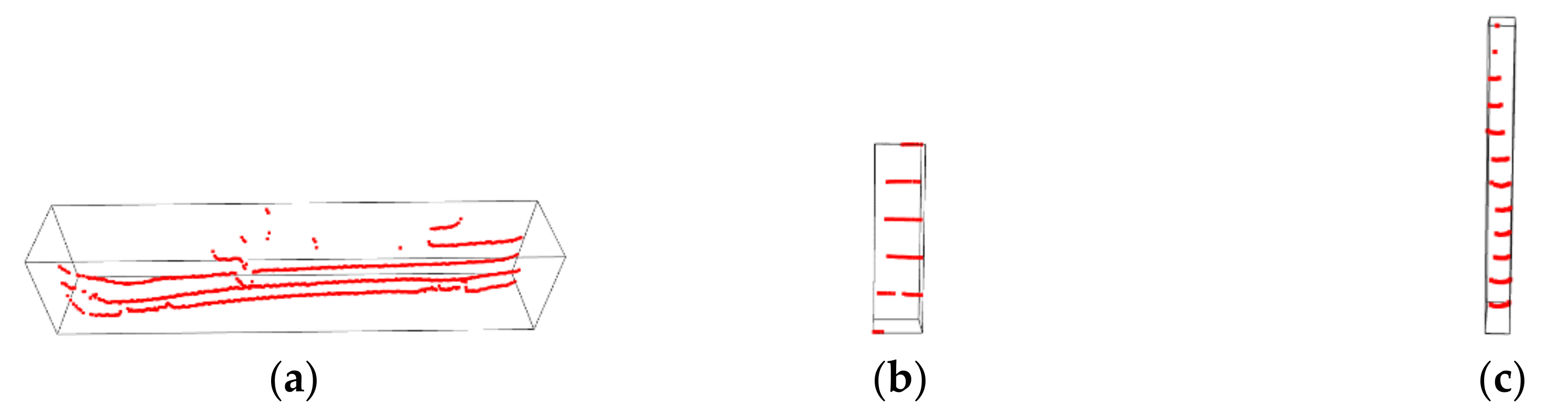
Figure 12.
Using the axis-aligned bounding box (AABB) formed by the major part to represent a certain object. (a) AABB of car; (b) AABB of pedestrians; (c) AABB of tree trunks.
Figure 12.
Using the axis-aligned bounding box (AABB) formed by the major part to represent a certain object. (a) AABB of car; (b) AABB of pedestrians; (c) AABB of tree trunks.

Figure 13.
Intersection of a moving object. (a) The intersection of the two sequence frames of point cloud data; (b) The intersection formed by the axis-aligned bounding box.
Figure 13.
Intersection of a moving object. (a) The intersection of the two sequence frames of point cloud data; (b) The intersection formed by the axis-aligned bounding box.

Figure 14.
The intersection over minimum volume (IOMin) of different objects in the current frame and the first five frames, respectively.
Figure 14.
The intersection over minimum volume (IOMin) of different objects in the current frame and the first five frames, respectively.

Figure 15.
The intersection over minimum volume (IOMin) of different objects in the current frame and the first five frames, respectively.
Figure 15.
The intersection over minimum volume (IOMin) of different objects in the current frame and the first five frames, respectively.

Figure 16.
The results of model training and prediction. (a) Overall accuracy and recall of labeling road users by the proposed model; (b) The results of labeling road users in the point cloud, where blue objects are road users and gray objects are static objects.
Figure 16.
The results of model training and prediction. (a) Overall accuracy and recall of labeling road users by the proposed model; (b) The results of labeling road users in the point cloud, where blue objects are road users and gray objects are static objects.

Figure 17.
The process of labeling static objects.

Figure 18.
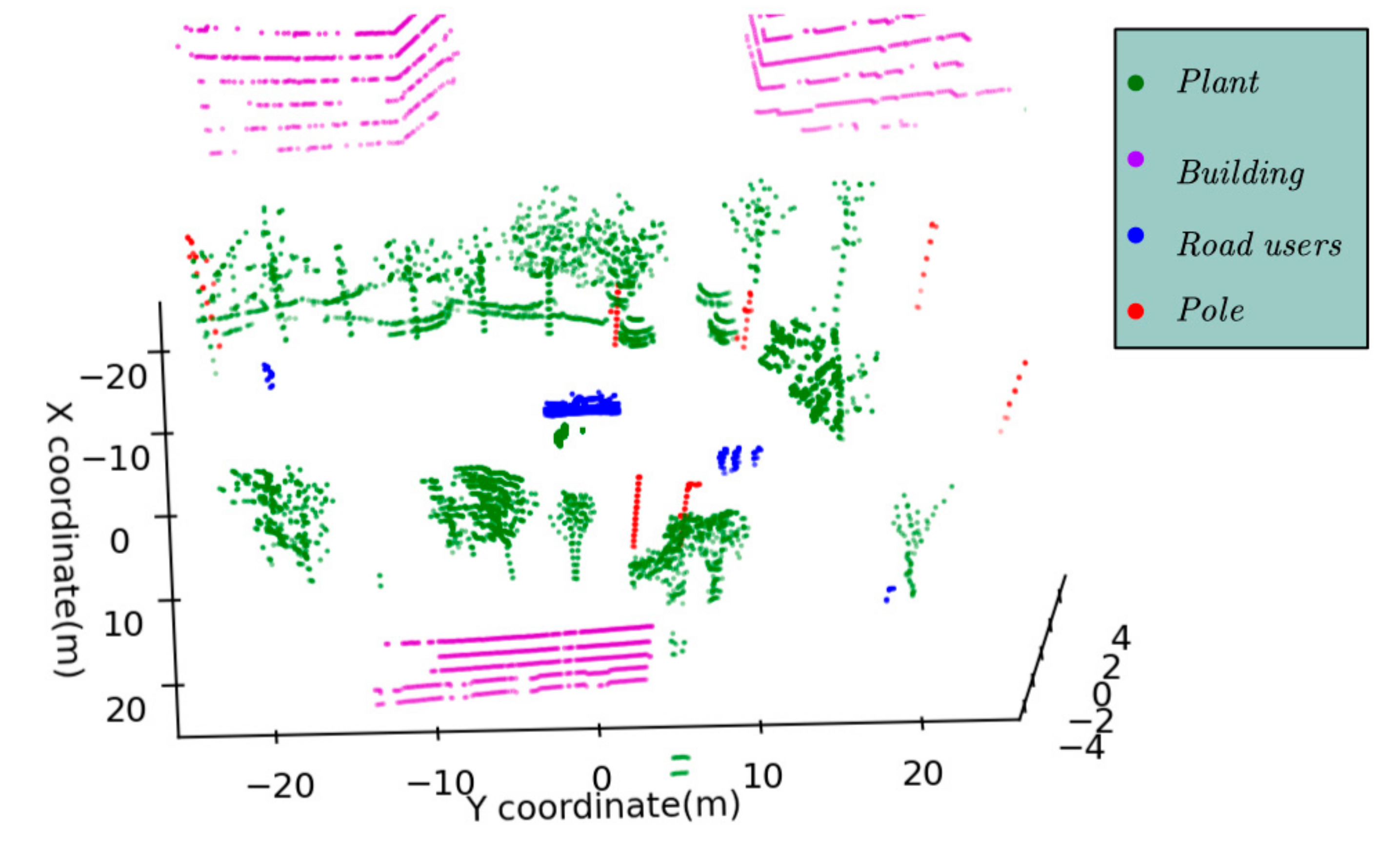
The results of semantic segmentation, where green objects belong to plants, violet objects belong to buildings, blue objects belong to the road users, and the red objects belong to poles.
Figure 18.
The results of semantic segmentation, where green objects belong to plants, violet objects belong to buildings, blue objects belong to the road users, and the red objects belong to poles.

Figure 19.
Aerial photography of the installation site.

Figure 20.
The results of different segmentation algorithms on an example point cloud are shown in LiDAR 360 software. Different colors in the original point cloud mean different heights. Different colors in the segmentation result mean different objects. (a) The raw point cloud before segmentation; (b) The results of instance segmentation by a Euclidean-based segmentation; (c) The results of instance segmentation by the regional growth algorithm in the Point Cloud Library (PCL); (d) The results of instance segmentation by the proposed algorithm.

Figure 21.
The results of semantic segmentation. (a) Original point cloud, where color means the height of points; (b) The results of semantic segmentation, where green objects belong to plants, violet objects belong to buildings, blue objects belong to the road users, and the red objects belong to poles.

Figure 22.
The results of the robustness experiment. (a) Aerial photography of the installation site at Location 2; (b) Original point cloud, where color means the height of points; (c) Results of instance segmentation, where colors are randomly generated and different colors of adjacent objects mean different classes; (d) Results of semantic segmentation, where green objects belong to plants, violet objects belong to buildings, blue objects belong to the road users, and the red objects belong to poles.


Table 1.
The number of objects before and after segmentation.
| Algorithms | Truth Number of Objects in the Original Point Cloud | Number of Objects after Segmentation |
|---|---|---|
| Euclidean-based | 59 | 12 |
| Regional growth in PCL | 29 | |
| Our work | 51 |
Table 2.
The effect of different IOMin sequence length on road user detection.
| IOMin Sequence Length | Accuracy | Precision | Recall | AUC |
|---|---|---|---|---|
| 1 | 0.7382 | 0.3391 | 0.8939 | 0.8445 |
| 2 | 0.8155 | 0.4306 | 0.9394 | 0.943 |
| 3 | 0.8991 | 0.5872 | 0.9697 | 0.9769 |
| 4 | 0.9464 | 0.7253 | 0.99 | 0.9889 |
| 5 (selected) | 0.9871 | 0.9167 | 0.9903 | 0.9952 |
| 6 | 0.9883 | 0.9228 | 0.9921 | 0.9934 |
Table 3.
The effect of different algorithms.
| Algorithm | Accuracy | Precision | Recall | AUC |
|---|---|---|---|---|
| K-means | 0.9112 | 0.6077 | 0.8874 | 0.901 |
| Spectral Clustering | 0.9373 | 0.7294 | 0.8212 | 0.8879 |
| Support Vector Machine (SVM) | 0.8283 | 0.2888 | 0.2219 | 0.5702 |
| Isolation Forest | 0.7974 | 0.3893 | 0.99 | 0.8794 |
| Artificial Neural Network (ANN) | 0.9678 | 0.8148 | 0.99 | 0.993 |
| Our work | 0.9871 | 0.9167 | 0.9903 | 0.9952 |
Table 4.
The Average Precision (AP) comparison of two unsupervised methods.
| Algorithm | Plant | Pole | Building |
|---|---|---|---|
| Spectral Clustering | 0.9573 | 0.8394 | 0.8012 |
| K-means (selected) | 0.9638 | 0.8646 | 0.826 |
Table 5.
The number of objects before and after instance segmentation.
| Object | Before | After |
|---|---|---|
| Road users | 7 | 7 |
| Plant | 3 | 2 |
| Pole | 5 | 3 |
| Building | 4 | 4 |
Table 6.
The average classification precision of each object.
| Object | Average Precision |
|---|---|
| Road users | 0.9902 |
| Plant | 0.821 |
| Pole | 0.8507 |
| Building | 0.7562 |
Publisher’s Note: MDPI stays neutral with regard to jurisdictional claims in published maps and institutional affiliations. |
© 2020 by the authors. Licensee MDPI, Basel, Switzerland. This article is an open access article distributed under the terms and conditions of the Creative Commons Attribution (CC BY) license (http://creativecommons.org/licenses/by/4.0/).
Share and Cite
MDPI and ACS Style
Liu, H.; Lin, C.; Wu, D.; Gong, B. Slice-Based Instance and Semantic Segmentation for Low-Channel Roadside LiDAR Data. Remote Sens. 2020, 12, 3830. https://0-doi-org.brum.beds.ac.uk/10.3390/rs12223830
AMA Style
Liu H, Lin C, Wu D, Gong B. Slice-Based Instance and Semantic Segmentation for Low-Channel Roadside LiDAR Data. Remote Sensing. 2020; 12(22):3830. https://0-doi-org.brum.beds.ac.uk/10.3390/rs12223830
Chicago/Turabian StyleLiu, Hui, Ciyun Lin, Dayong Wu, and Bowen Gong. 2020. "Slice-Based Instance and Semantic Segmentation for Low-Channel Roadside LiDAR Data" Remote Sensing 12, no. 22: 3830. https://0-doi-org.brum.beds.ac.uk/10.3390/rs12223830
Note that from the first issue of 2016, this journal uses article numbers instead of page numbers. See further details here.