Article

Quality Assessment of Photogrammetric Methods—A Workflow for Reproducible UAS Orthomosaics

1
Department of Geography, Philipps-University Marburg, Deutschhausstr. 10, 35037 Marburg, Germany
2
GAMES Group, Department of Horticulture, Fruit, Growing Botany and Gardening, University of Lleida, 25198 Lleida, Spain
3
Swiss Federal Institute for Forest, Snow and Landscape Research WSL, Zürcherstr. 111, 8903 Birmensdorf, Switzerland
4
Geoscience Barcelona (GEO3BCN—CSIC), 08028 Barcelona, Spain
5
Laboratory ECOFUN, Forest Science and Technology Centre of Catalonia (CTFC), 25280 Solsona, Catalonia, Spain
*
Author to whom correspondence should be addressed.
Remote Sens. 2020, 12(22), 3831; https://0-doi-org.brum.beds.ac.uk/10.3390/rs12223831
Submission received: 21 October 2020 / Revised: 15 November 2020 / Accepted: 19 November 2020 / Published: 22 November 2020
(This article belongs to the Special Issue UAV Photogrammetry and Remote Sensing)

Abstract

:
Unmanned aerial systems (UAS) are cost-effective, flexible and offer a wide range of applications. If equipped with optical sensors, orthophotos with very high spatial resolution can be retrieved using photogrammetric processing. The use of these images in multi-temporal analysis and the combination with spatial data imposes high demands on their spatial accuracy. This georeferencing accuracy of UAS orthomosaics is generally expressed as the checkpoint error. However, the checkpoint error alone gives no information about the reproducibility of the photogrammetrical compilation of orthomosaics. This study optimizes the geolocation of UAS orthomosaics time series and evaluates their reproducibility. A correlation analysis of repeatedly computed orthomosaics with identical parameters revealed a reproducibility of 99% in a grassland and 75% in a forest area. Between time steps, the corresponding positional errors of digitized objects lie between 0.07 m in the grassland and 0.3 m in the forest canopy. The novel methods were integrated into a processing workflow to enhance the traceability and increase the quality of UAS remote sensing.

Graphical Abstract

1. Introduction

Unmanned aerial systems (UAS) are widely used in environmental research. Applications encompass the retrieval of crop yield [1] or drought stress [2] in agricultural areas or the mapping of plant species [3,4,5], biomass [6,7] or forest structure [8,9,10] in nature conservation tasks. Today, UAS allow an extensive spatial coverage with high resolution that provides detailed observations on the individual plant level, e.g., for the detection of pest infections in trees [11] or rotten stumps [12]. The flexibility of UAS is also beneficial for multi-temporal observations since flights can be scheduled on short notice based on specific events like bud burst or local weather conditions. Therefore, UAS are regarded as a key component for bridging the scales between space-borne remote sensing systems and in-situ measurements in environmental monitoring systems [13].
Applications of UAS can be structured into two main components: the acquisition of individual images—including the flight planning—with an unmanned aerial vehicle (UAV) for a particular region of interest and the processing of these images with photogrammetric methods to obtain georeferenced orthophoto mosaics [8,14,15,16] or digital surface models [8,17,18]. Studies on the development of workflows for UAS are sparse, often exclude the flight planning and are mostly tied to a very specific application [4,19]. A generalized, flexible and commonly accepted workflow is still missing [13].
Standardized protocols and quality assessments are needed for a better understanding and appropriate use of UAS imagery. Since the final product quality depends on the initial image capturing, flight planning is one important aspect in a common workflow scheme. For example, the flight height in conjunction with the used sensor (RGB, multispectral or hyperspectral) affect the ground sampling distance (GSD, i.e., pixel size or spatial resolution) of the images and in conjunction with the flight path affect the overlap of the individual images which is a key factor for the successful image processing [20]. A fully reproducible study therefore must include the flight path and parameters as well as the camera configuration metadata. For ready-to-fly consumer UAV, flight planning is usually done in software which is tied to the specific hardware (e.g., the DJIFlightPlanner for DJI drones). These commercial solutions often do not provide the full control of autonomous flights and access to metadata which makes it difficult to integrate flight planning in a generalized workflow. In this respect, open hardware/software solutions like Pixhawk based systems and the MAVlink protocol (mavlink.io) are advantageous. To complete the metadata, environmental conditions during the flight like sun angle and cloudiness that also have impacts on the image quality [21] should be recorded.
Equally or even more important for valid results and their use in subsequent data analysis or synthesis is a quality assessment of the resulting image products in terms of their spatial accuracy and reproducibility. The basic image processing workflow starts with the alignment of the individual images, which results in a projected 3D point cloud. Usually, this point cloud is georeferenced through the individual image coordinates or via the use of measured ground control points (GCPs) [22,23]. The point cloud is the basis for the generation of a surface model and the orthorectification and mosaicing of the individual images based on this surface. Commercial software such as Metashape (Agisoft LLC, St. Petersburg, Russia; formerly known as Photoscan) makes these complex photogrammetric methods accessible to a broad range of users and has been utilized in numerous studies [3,13,24].
The quality of photogrammetrically compiled orthomosaics is commonly expressed as their georeference accuracy [25,26,27,28] or statistical error metrics derived from the image alignment (e.g., the amount of points in the point cloud or the reprojection error [8,29]). However, these measures alone provide no comprehensive information about the quality of the orthomosaic since the subsequent steps of orthorectification and mosaicing are not taken into account. Image artifacts and distortions can occur during these processing steps that are not reflected in the georeference accuracy [30]. Especially in forest ecosystems, the complex and diverse structures and similar image patterns in the canopy can lead to erroneous imagery [20]. In addition, wind exposure leads to changes in the structure of the tree canopy and consequently causes problems in the alignment of individual images [31]. The quality assessment becomes even more important when time series are analyzed since actual changes of the observed environmental variables have to be separated from deviations which stem from the image processing itself. In addition, here low georeferencing errors are even more important since the errors of the individual time steps can accumulate. Studies utilizing time series relied on georeferencing errors below 10 cm of the individual time steps [26,32].
To evaluate the reproducibility and validity of orthomosaic time series, it is therefore necessary to: (1) optimize the positional accuracy of the individual orthophoto mosaics, (2) to evaluate the reproducibility of the photogrammetric processing of these orthophoto mosaics and (3) to evaluate the positional accuracy between features in the individual time steps of the series.
This study proposes (i) an optimization for the orthorectification of UAS images and (ii) an additional quality criterion for UAS orthomosaics that focuses on the reproducibility of the photogrammetric processing. The orthorectification is improved by an automated optimization of the checkpoint error based on an iteration of point cloud filters. The reproducibility of orthomosaics is quantified by the repeated processing of the same scene and a pixel-wise correlation analysis between the resulting orthophoto mosaics. We illustrate the importance of both methods using different orthorectification surfaces and two time series in a grassland and a forest area, respectively. To foster an error and reproducibility optimized orthomosaic processing, we incorporate the new methods into an impoved UAS workflow.

2. Materials and Methods

2.1. Multi-Temporal Flights

Two multi-temporal UAV-based image dataset were acquired as a test sample for this study (Table 1). The first dataset is a series of six consecutive flights over a small temperate forest patch (Wolfskaute, Hesse, Germany). The surveyed area covers 7 ha of a forested hill with an adjacent meadow and ranges from 283 m to 320 m a.s.l. (above sea level). with a canopy height of up to 37 m (Figure 1a). The six flights were performed on 2020-07-07 between 11:00 and 14:00 CEST using a 3DR Solo Quadrocopter (3D Robotics, Inc., Berkeley CA, USA) and a GoPro Hero 7 camera (GoPro Inc., San Mateo, CA, USA; Appendix B, Table A1). The flight plan was made with Qgroundcontrol and refined with a LiDAR derived digital surface model (DSM, provided by the Hessian Agency for Nature Conservation, Environment and Geology (HLNUG)) with the R-package uavRmp to achieve a uniform altitude of 50 m above the forest canopy (see Appendix A). For georeferencing and checkpoint error calculation, 13 ground control points (GCPs) were surveyed with the Real Time Kinematic (RTK) GNSS (Global Navigation Satellite System) device Geomax Zenith 35 (GeoMax AG, Widnau, Switzerland). The RTK GNSS measurements had an error of between 0.9 and 1.6 cm in the horizontal direction and between 1.9 and 3.7 cm in the vertical direction. Eight GCPs were used as controlpoints and five served as independent checkpoints to evaluate the georeferencing error (Figure 1a).
The second dataset is an inter-annual time series of a grassland area (La Bertolina, Eastern Pyrenees, Spain). Terrain altitudes range from 1237 m to 1328 m a.s.l. The flights were performed in spring or early summer of 2013, 2015 and 2017 using an octocopter with a Pixhawk controller. Cameras and flight plans in a fixed altitude differ between the dates (Table 1), detailed camera settings in Appendix B, Table A1). The flights took place in the morning with sub-optimal illumination angles below 35 degrees [21] and partly scattered light conditions due to the presence of clouds. Five to eight GCPs were measured in each year with a conventional GPS device without RTK, from which three were used as checkpoints (Figure 1b).
Both datasets were used to empirically determine the georeferencing accuracy and reproducibility of the photogrammetrically retrieved orthomsoaics. For a better understanding of the newly introduced approaches, the following chapters first outline the general UAS image processing workflow.

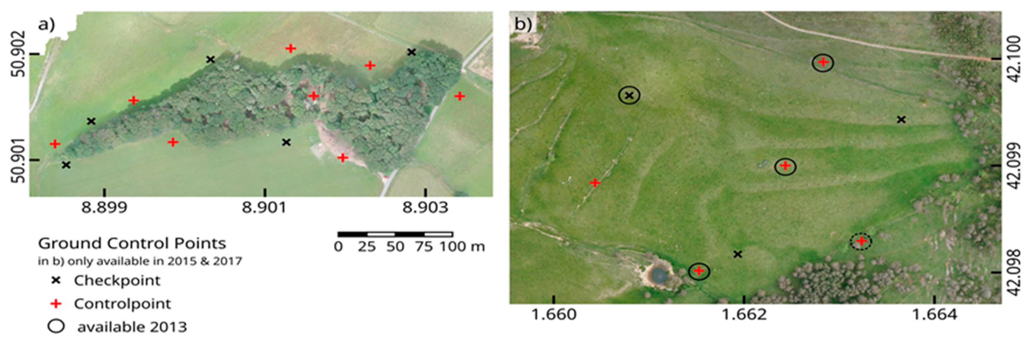
2.2. Image Georeferencing

Very high resolution orthomosaics such as those resulting from UAV flights require precise positioning to avoid the introduction of complex errors in the image processing [33]. The standard GNSS receivers that are built in cameras do not provide sufficient accuracy. There are two alternative strategies for georeferencing the UAS products: direct georeferencing of the images with a RTK on the UAV or the use of GCPs. Direct georeferencing requires the accurate time synchronization between the RTK device and the camera, which has been reported as a major source of error [33,34,35].
The use of GCP implies that the study area is accessible in order to install visible ground markers before the flight and precisely measure their position. Ideally, the GCP should be equally distributed over the study area to avoid distortions during processing [33]. During the orthomosaic processing, the ground markers need to be interactively identified in the images. Despite these drawbacks, georeferencing through GCP with general-purpose GNSS receiving systems—that are nowadays standard equipment for surveying—is still far more widespread and potentially more cost-effective than the direct georeferencing with RTK [34].
In any case, GCPs are also required for the independent validation of the referencing accuracy during the processing [24] and therefore essential for a proper accuracy assessment. The geolocation accuracy is usually given as the checkpoint root mean squared error (checkpoint error, Equation (1)) that quantifies the distance between the position of the measured GCP (XYZgcp) and the estimated positions of these coordinates in the photogrammetric processing (XYZest). It can be calculated for each direction individually.
C h e c k p o i n t e r r o r = m e a n ( ( X Y Z g c p X Y Z e s t ) 2 )

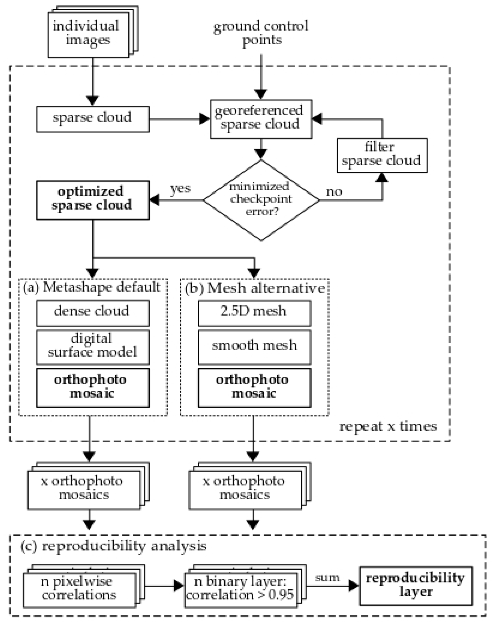
2.3. Photogrammetric Processing

The Metashape software (Agisoft LLC, St. Petersburg, Russia; formerly known as Photoscan) is widely used for UAS image processing. The standard photogrammetric workflow includes the image alignment, the generation of a digital surface model (called Digital Elevation Model in Metashape) and the orthorectification and mosaicing (Figure 2). The image alignment starts with the automatic identification of distinct features in the individual images. This process is enhanced and requires less computation time if the individual images already contain GNSS information. Those features which appear in more than one image, the so called tie points, are matched and projected in a 3D space, forming the sparse cloud that is georeferenced using the surveyed GCPs. The georeferenced sparse cloud is subsequently used to compute a digital surface model, either through a dense pointcloud or a mesh interpolation of the sparse cloud (Figure 2a,b). The surface model is finally used for rectifying the georeferenced images.
For each processing step, a multitude of parameters and options are available that affect the results in terms of georeferencing accuracy and orthomosaic quality. While Metashape offers default values for these parameters, the methods described below aim to optimize and alter the standard workflow to obtain high quality and reproducible orthomosaics.

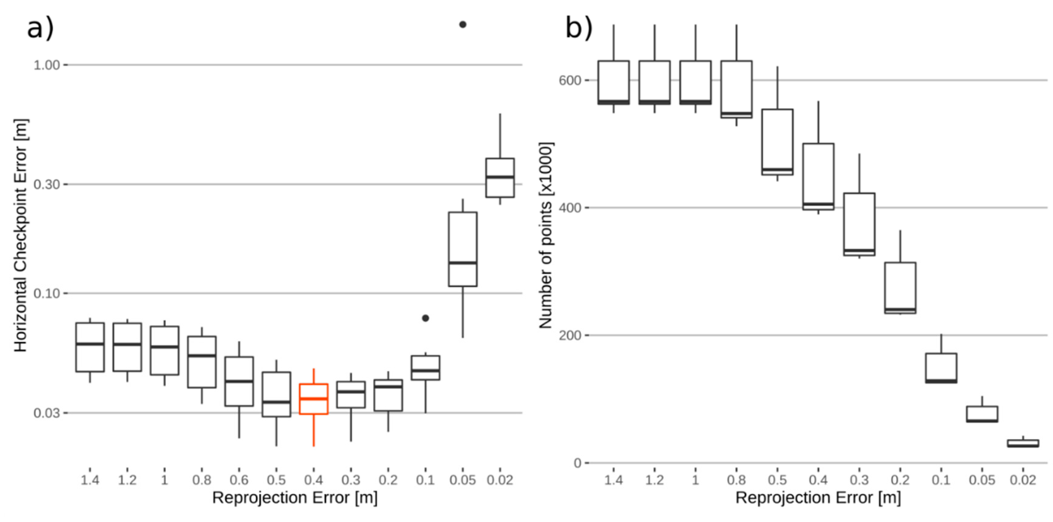
2.4. Optimizing the Georeferencing

Each point in the sparse cloud has four accuracy attributes: the reconstruction accuracy (RA), the reprojection error (RE), the projection accuracy (PA) and the image count [35]. In particular, the RE is suggested as the quality measure of tie points [20,36]. It is the deviation of the positions of identified features in the original image from positions of the same features in the calculated 3D space. The removal of points with a high error and the subsequent optimization of the camera positions can improve the georeferencing. However, by removing too many points in the individual sparse clouds, images no longer align and the checkpoint error increases. An iterative approach is used to find the optimal RE threshold for the dataset by filtering the sparse cloud using different RE threshold values in order to minimize the checkpoint error (Figure 2). This method was applied to each flight of the two multi-temporal datasets.
The initial pointclouds are the direct results from the feature identification and matching algorithms from Metashape. In order to account for the inherited randomness of these processes and the slight differences of the checkpoint error due to the manual alignment of the GCP, the optimization was repeated five times and the standard deviation of the checkpoint error was calculated.

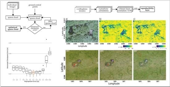
2.5. Orthomosaic Reproducibility

Since the orthomosaics are the result of complex photogrammetric methods, its reproducibility has to be assessed. In this context, reproducibility is a measure of how identical individual orthomosaics are, if they are computed from the same image source and with identical photogrammetric processing parameters. This way, the reproducibility of the photogrammetric process itself is evaluated without the influence of changes in the surveyed environment. For this purpose, a set amount of orthomosaics is computed with identical settings (Figure 2). To quantify the reproducibility, the pixel-wise correlation coefficient of the RGB values is calculated between each pair of the computations (raster R package, corLocal function). Pixels with a correlation coefficient of 0.95 or higher are considered identical between two orthomosaics. This leads to a binary layer for all pair-wise correlations marking reproducible and non-reproducible pixels. By summing up the binary layers, regions of high and low reproducibility can be identified (Figure 2c). High values then denote a high level of reproducibility of a pixel.
The more orthomosaics are computed, the more correlation layers can be calculated (Equation (2)) and the more likely a layer is to receive a non-correlating pair of pixels. Therefore, a preliminary test with an arbitrarily high number of 25 orthomosaics (x = 25) was done, which leads to n = 300 correlation layers.
n c o r r e l a t i o n s = x ! 2 ! ( x 2 ) !
In practice, computing 25 orthomosaics is, in most cases, unreasonable regarding the computation time and processing resources. Therefore, the reproducibility analysis was also done with only 5 identical orthomosaic computations (i.e., 10 pairwise correlations). The comparison of both reproducibility layers revealed that summing up 10 correlation layers (x = 5) is sufficient to identify most pixels which are also denoted as non-reproducible when using 300 binary layers. The analysis of the time series and the full forest set were therefore done with only 5 identical orthomosaic computations.
In addition, the edges of the orthomosaic are heavily distorted and have a lower positional accuracy due to less image overlap [37]. Therefore, the orthomosaic should be cropped to the central area with a sufficient overlap. In the R package uavRmp provided with this study, this crop mask is automatically generated from spatial polygons defined by the seamlines (i.e., the outline of the individual image parts) of the mosaic. The outermost polygons are identified using a concave hull of the seamlines and are discarded from the orthomosaic.
All computations were done in R (Version 4.0.2; [38]). All presented methods are provided as the R-package uavRmp (https://gisma.github.io/uavRmp/) and the Metashape Python Scripts (https://github.com/envima/MetashapeTools).

2.6. Assessing the Orthorectification Surface

The standard workflow in Metashape suggests a DSM created from a dense pointcloud as the orthorectification surface (Figure 2a) [16]. In vegetation free areas, this DSM is mostly equivalent to a digital elevation model (DEM) [39] or digital terrain model (DTM) and therefore suitable for the creation of orthomosaics. In areas with vegetation, the DEM requires the classification of ground points in the dense pointcloud which is currently not viable in Metashape for structurally rich environments like forests or grasslands in the phases of maturation and flowering. Alternatively, a 2.5D mesh can be created from the sparse cloud on which the images are projected [40]. By smoothing the mesh to eliminate sharp edges, the surface can be regarded as an approximation of a DEM. This approach requires far less computational ressources since the creation of a densecloud is skipped. It is therefore more suitable for low-budget UAS setups. To demonstrate and validate its usage, the mesh surface was compared to the DSM for one of the forest scenes with respect to the reproducibility of the derived orthomosaics using the pixel-wise correlation method described above.

2.7. Time Series Accuracy

To assess the overall reproducibility of time series, reproducibility masks have been computed for each time step and overlaid to identify pixels that are reproducible over the multi-temporal data and suitable for time series analyses. To differentiate between positional errors from the photogrammetric processing and actual environmental changes between the time steps, identifiable objects and trees were digitized in each individual orthomosaic (7 geometries in the forest, 4 in the grassland). The positional shift of the bounding boxes for each digitized object was calculated between each time step. This provides a more critical assessment of time series than the individual checkpoint errors alone, since relative position differences and environmental changes between the time steps are taken into account.

3. Results

3.1. Optimized Georeferencing Accuracy

To evaluate the optimized georeferencing approach, the sparse clouds were iteratively filtered with decreasing RE thresholds. The sparse clouds of the six forest flights originally included between 560,000 and 680,000 tie points (Figure 3b) after the image alignment with a maximum initial checkpoint error of 3 m. The checkpoint errors were minimized to values between 0.021 and 0.046 m if a RE threshold of 0.4 m was used (Figure 3a). The corresponding pointclouds consisted of about 150,000 tie points. Further reducing the RE threshold to 0.1 m increased the checkpoint error (Figure 3b) due to an insufficient number of tie points for image alignments.
In order to test the robustness of the method, the determined optimal RE threshold of 0.4 m was used to filter the sparse clouds of five identical computations of the six forest flights. The average controlpoint error in the horizontal direction was consistently below 0.02 m in all six flights and deviated less than 0.001 m in each of the five computations. The horizontal checkpoint error was between 0.02 m and 0.06 m over all six flights and deviated less than 0.01 m within the five computations. The error in the vertical direction (Z in Table 2) was up to five times higher; however, the reproducibility in each flight is still stable with a maximum deviation of 0.03 m over the five computations.
In the grassland area, the iterative point cloud filtering only marginally improved the checkpoint error since almost all tie points had already very low RE of less than 0.4 m. The final checkpoint errors for the years 2013, 2015 and 2017 were 0.29 m, 0.18 m and 0.07 m, respectively. These errors are up to 10 times higher than in the forest time series, which is mostly due to the use of a conventional GNSS measurements for the GCP in the grassland compared to the RTK GNSS measurement in the forest. Nevertheless, the five computations of the grassland time series led to very consistent checkpoint errors with standard deviations close to 0 (Table 2).

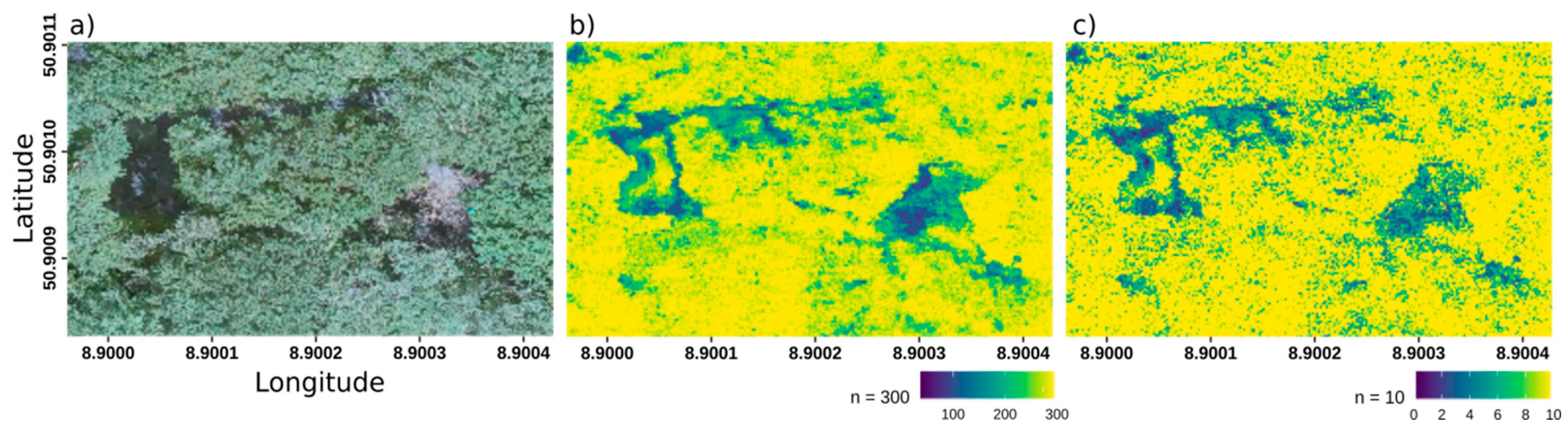
3.2. Orthomosaic Reproducibility

To evaluate the reproducibility of orthomosaics, the images of the 4th forest flight were computed 25 times with identical photogrammetric parameters. The 300 pixel-wise correlation analysis between the 25 orthomosaics were performed within a testing area of 600 by 650 pixels showing the forest canopy (Figure 4a). Pixels with correlation coefficients higher than 0.95 were considered reproducible between the orthomosaics. Highly reproducible pixels are characterized by consistently high correlation coefficients and therefore high values in the summed up layer shown in Figure 4b. Non-reproducible regions appear mainly in forest clearings or at dead trees. The actual canopy appears stable across multiple computations.
Using only five identical orthomosaics (i.e., 10 pairwise correlation analyses, Figure 4c) revealed the same patterns as the 300 correlation layers. Hence, only five repetitions are considered enough for subsequent reproducibility analyses.

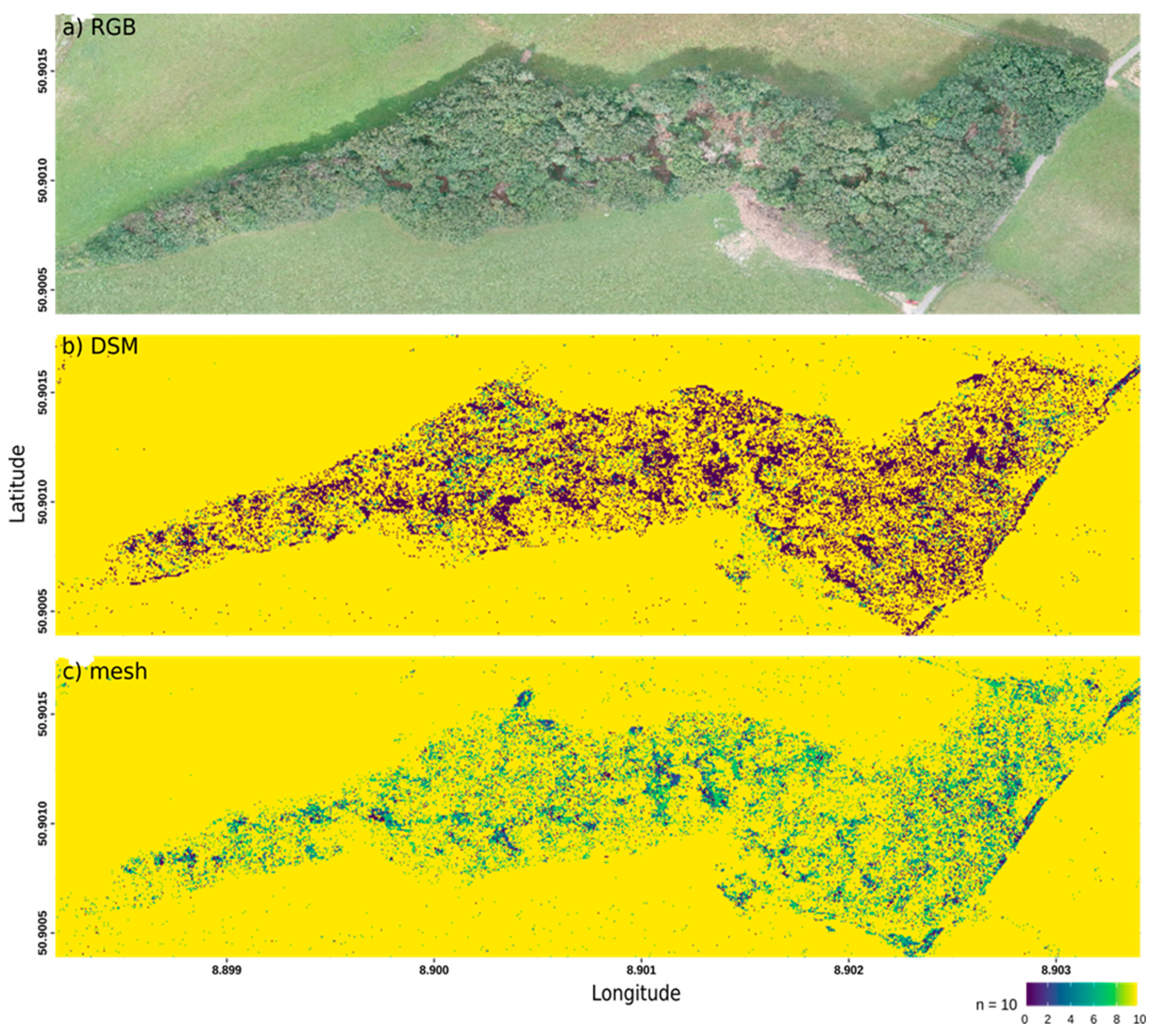
3.3. Comparison of Mesh and DSM Surface-Based Orthomosaics

To evaluate to which degree the reproducibility of orthomosaics depends on the use of the underlying mesh and DSM surface in the forest environment, both surfaces have been used in otherwise identical computation workflows. Using 5 identical orthomosaic computations, 82% and 85% of the pixels were considered reproducible using the DSM and mesh, respectively. All non-reproducible pixels were found in the forest clearing areas of the images. The surrounding meadow did not differ between the orthomosaics (Figure 5). When only the forested area is considered, the number of reproducible pixels decreased to 69% in the DSM and 74% in the mesh-based processing.
While being nearly identical in their amounts of reproducible pixels, there is still a large contrast between the orthomosaic reproducibility of the two surfaces. If a pixel in the DSM-based orthomosaics is non-reproducible between two images, there is a high probability that this pixel is non-reproducible in all images (Figure 5). The mesh-based orthomosaics show significantly more pixels that are non-reproducible between only one or two different orthomosaics, but were stable between the other computations.

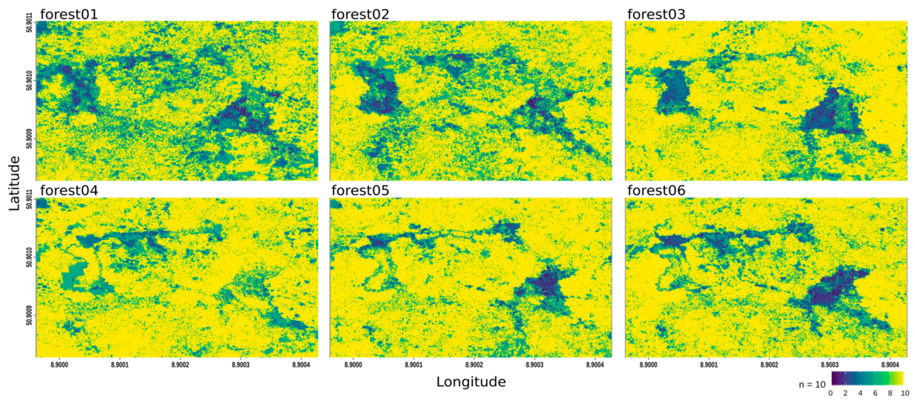
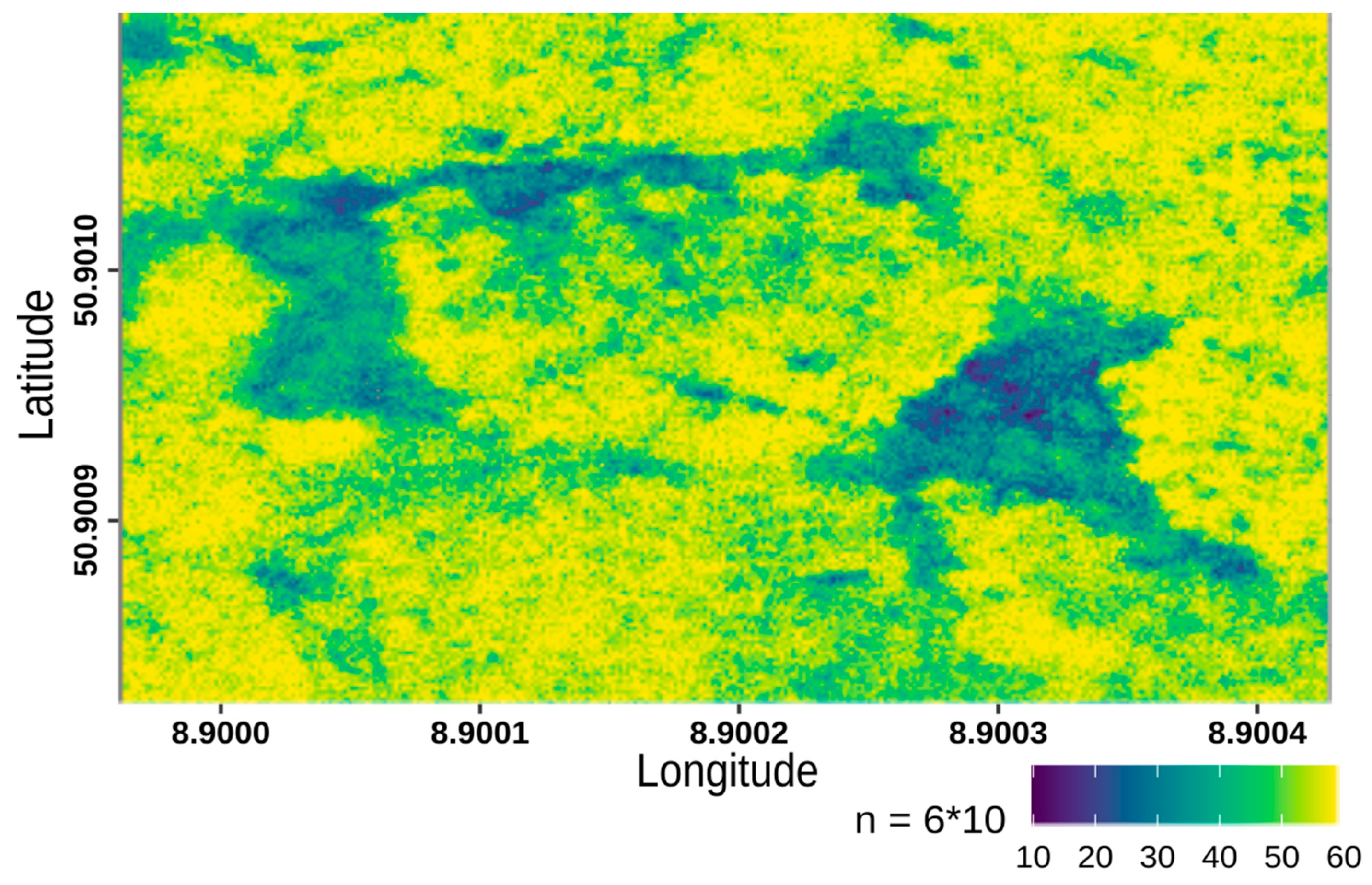
3.4. Forest Time Series Reproducibility

The same canopy part of the orthomosaics as in Figure 4 was used for the assessment of the reproducibility along a time series. Figure 6 reveals that non-reproducible areas are mostly consistent between the flights. They concentrate around clearings and around the branches of dead crowns visible in Figure 4a. The actual forest canopy is reproducible. Flight conditions also seem to have an impact on the overall reproducibility. Forest 03 to 06 which were performed in cloudy conditions show less deviations between computations than Forest 01 and 02 where cloud-free conditions and low solar elevations are present.
Summing up all the correlation layers of the six flights (Figure 7) leads to a quality mask for the whole time series. This confirms that the canopy region is reproducible and stable even across the time series.

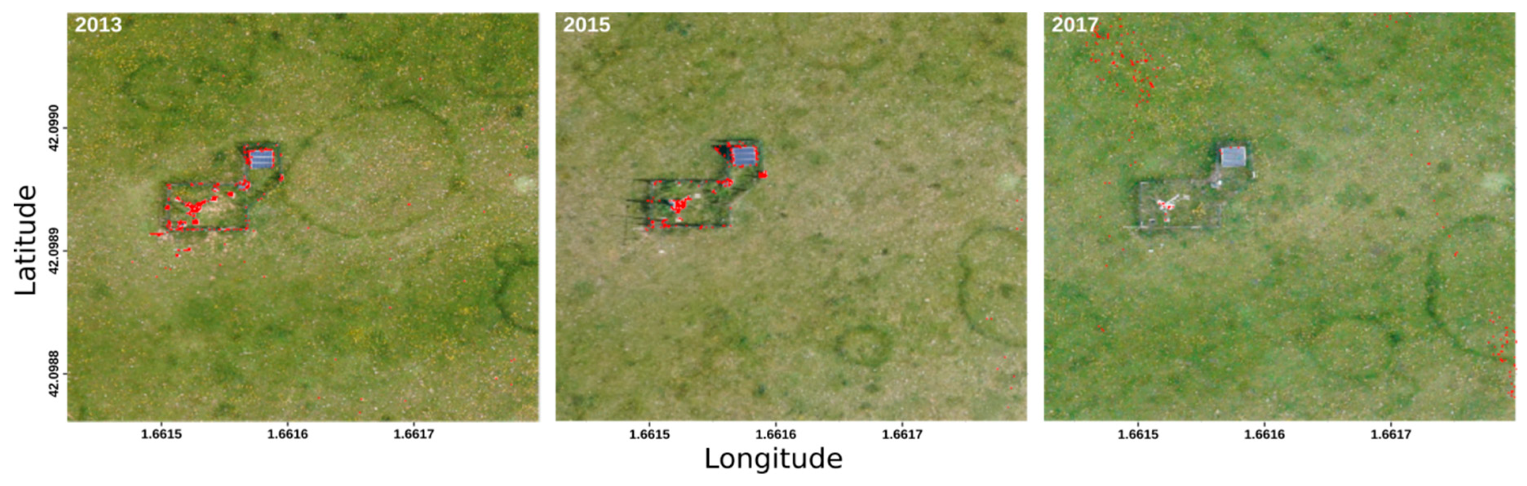
3.5. Grassland Time Series Reproducibility

In the grassland time series, the reproducibility of each orthomosaic was also tested with five identical computations. Only 1% of the pixels in the grassland area deviated between the computations of each year. In 2013 and 2015, the non-reproducible areas occur mainly in the area of a micrometeorological station in the middle of the meadow (Figure 8). In 2017 some singular pixels also deviated in the meadow areas.

3.6. Time Series Positional Accuracy

To further assess the validity of UAS time series, the positional shift between 7 digitized tree crowns in the forest and four visible objects in the grassland were calculated. Tree crowns moved by 0.3 m on average with a maximum shift of 0.75 m of one tree between forest flight 02 and 03. During the image acquisition of these two flights, the lighting conditions changed due to the presence of clouds and changing wind speeds. In Figure 9, the positional shift of 0.3 m to the left of the marked tree is visible as well as slight differences in the geometry of the crown due to different lighting conditions and wind.
The solar panel visible in Figure 6 is one of four objects which were digitized to measure the positional accuracy of the grassland time series. Between the individual time steps, on average, the polygons differed by 0.03 m in their position. The largest deviation occurred between the orthomosaics of 2013 and 2017 with a maximum shift of 0.07 m between one object. Hence, environmental changes in the grassland have less impact on the time series.

4. Discussion

The increasing use of UAS imagery in science and science-related services demands a operational processing and reliable validation techniques in the commonly used photogrammetric workflows. This study introduces two optimizations to the conventional photogrammetric workflow: (1) a new optimization for the georeferencing workflow and (2) a novel technique aiming to evaluate the repeatability of photogrammetrically retrieved orthomosaics. The application of these methods demonstrated the possibility to acquire accurately referenced UAS orthomosaic time series with low-cost UAVs and RGB cameras for both forest and grassland environments. The reproducibility of orthomosaics was highly dependent on the vegetation structure of the survey area.

4.1. Optimized Georeferencing Accuracy

The determination of optimal tie point filters leads to positional precisions of less than 6 cm in forested areas. Regarding the GSD of 2.58 cm/px the resulting orthomosaics have a positional error of up to three pixels. This error is stable over multiple computations and different sets of images from the six flights over the forest. This suggests that the iterative filtering approach leads to robust RE thresholds and only needs to be computed one time.
The difference of 0.04 m in the checkpoint error between the six flights could come from different GNSS satellite constellations or cloud conditions [41] over the three hours the flights took place, but, most likely, these small differences come from slight inaccuracies during the manual alignment of the GCP. This suggests that the operational workflow consistently leads to viable orthomosaics with resolutions of less than 10 cm, which is more than sufficient for detailed spatio-temporal structural analysis of forests [9,10]. In Belmonte et al. [8], a checkpoint error of 1.4 m and a GSD of 15 cm led to validated object-based analysis even in moderately dense canopies. The accuracy in the experimental forest areas even keep up with the checkpoint error in the grassland time series (between 0.04 m and 0.08 m). This also compares very well with other studies in structurally sparse landscapes where checkpoint errors tend to be very low [33,42].
The grassland time series further demonstrates that the proposed methods of optimization and validation work outside of the experimental setup. Differences in flight planning, low quality GNSS measurements at the GCP and the usage of different cameras still led to consistent and accurate orthomosaics. Hence, the provided workflow can be used as a fully operational method in grassland and agricultural contexts.

4.2. Pixel-Wise Reproducibility of Orthomosaics

The pixel-wise correlation of identically computed RGB orthomosaics leads to a quantitative measurement of reproducibility. This is a necessary addition to assess the photogrammetic processing of images, especially considering the “black box” nature of non-open-source software like Metashape. With the pixel-wise approach, deviations between computations are assigned to certain spatial regions of the orthomosaic. The mesh and DSM as orthorectification surfaces in the forest time series showed similar amounts of reproducible pixels (DSM: 69%, mesh: 74%). However, the mesh is considered superior since it leads to a better reproducibility in canopy areas. The calculation of the mesh is also less time consuming than the computation of the DSM. Both digital surfaces failed to reproduce fine structures like single tree branches or forest gaps. This can be problematic, since these structures are most likely the ones researchers aim to observe with UAS imagery [11,16,43].
The results also suggest that non-reproducibility can be tracked down to uncertainties in the initial step of the photogrammetric process, the feature identification and feature matching of the individual images [31]. These uncertainties increase with the presence of fine structures in the images since they are prone to move even under light wind conditions. It is therefore more likely that their position changes in consecutive images. In particular, Döpper et al. (2020) [44] recently demonstrated that acquiring UAV data for forest, grasslands and crop environments in low-light conditions such as low Solar Elevation Angle or high cloud cover causes problems in matching characteristics in the image alignment process.
Although this study declares these areas as not reproducible, the structures are still apparent in the orthomosaics. Image analysis methods (e.g., an object-based classification) of these areas might still lead to viable results and consistent geometries. This should be investigated in subsequent studies.

4.3. Time Series

The combination of multiple reproducibility layers enables the validation of UAS derived orthomosaic timeseries. The high reproducibility of multi-temporal grassland orthomosaics confirms the valid analysis of vegetation dynamics in grassland and agricultural studies. Forested area time series are also possible, however non-reproducible regions have to be considered.
The checkpoint error of each orthomosaic in the time series alone gives no insight into the positional relation between the individual time steps. Image acquisition with the UAV, analysis tools (processing software), field experiment designs and environmental conditions have a strong impact on the geometric accuracy of photogrammetric products [6,45,46]. Hence, it is essential to quantify the geometric accuracy on aerial imagery when combining UAS data from different flights, dates and sources [47]. We suggest the addition of geometry-based deviations from digitized objects. In case of the grassland time series, a maximum positional shift of 0.07 m between the time steps is tolerable for most use cases such as the modelling of the temporal dynamics of biophysics and biochemical variables of the meadow canopy or even analyze the variability in size and distribution of vegetation patterns (Lobo et al. in prep). This error also lies in the range of the individual checkpoint errors (0.04 to 0.08 m). In the forest time series, similar accuracies were achieved in the surrounding meadow areas. However, the canopy showed positional deviations of up to 0.5 m in digitized trees. A proportion of this error comes from the actual movement of the canopy due to wind and changes in the lighting conditions [44]. The non-reproducibility of some parts of the canopy, especially at forest clearings may also contribute to this error. We suggest object-based analysis instead of pixel-based approaches when high-resolution forest time series are regarded.

4.4. Improved UAS Workflow

The suggested methods of checkpoint error optimization and reproducibility validation complement the general UAS workflow. In order to make these methods more accessible to users, we provide a Python module—MetashapeTools (https://github.com/envima/MetashapeTools)—which utilizes the Metashape API for an improved photogrammetric workflow. The orthomosaic processing in form of a script-based workflow ensures the documented parameterization of all the modules in Agisoft Metashape. The workflow is therefore shareable and can be easily integrated into a version control system, making UAS research more transparent. Apart from the manual alignment of the GCP, the photogrammetric process is fully automated. The default parameters in the MetashapeTools are the results of the experimental forest flights and a starting point for a multitude of flight areas. The script-based framework provides flexibility to alter different parts of the workflow and, e.g., integrate alternative processing steps for time series like in Cook et al. [48].
In the future, the general workflow should utilize only open-source software. Currently, Agisoft Metashape is the de facto standard and the most promising software in affordable UAS image processing [3,13]. The development of open-source photogrammetry projects like OpenDroneMap are promising and will be integrated once they are fully operational. The transition from proprietary software towards open and transparent workflows is an ongoing trend worth supporting in spatial analyses [49]. For now, publications utilizing Metashape or other “black box” software should at least include the checkpoint error and the full parameterization of the processing modules. Ideally, the parameterization can be provided as a script, e.g., as a supplementary material or published in a repository. Although the computation of the reproducibility layer can be intensive, its inclusion in studies provide the necessary transparency about the quality and interpretation of the orthomosaics. The documented and evaluated orthomosaics are a big contribution to environmental mapping and monitoring system [50].

5. Conclusions

The rising popularity of UAS imagery in all fields of spatial research led to a variety of processing approaches. The supposedly ease of use and low cost of ready-to-fly UAS opened up some pitfalls in the image acquisition and processing which this study addressed. The evaluation of the orthomosaic accuracy aimed at the reproducibility of the final product. The presented optimization of the georeferencing accuracy based on the checkpoint error and the quantification of the orthomosaic reproducibility enhance the UAS workflow with the necessary quality assessment. This complements the standardized acquisition of high quality UAS time series.
In forest environments, there are still some shortcomings of UAS orthomosaic reproducibility that quantitative analyses need to consider. In grassland environments, these issues are marginal, which supports the validity of UAS in agricultural applications. The novel approaches of this study and their incorporation into a workflow are promising for validated and transparent UAS reserach.

Supplementary Materials

Author Contributions

M.L. analyzed data, contributed to the study design, developed the methodology, and was the main writer of the manuscript; C.M.R. analyzed data (grassland), and contributed to the manuscript; N.F. contributed to the study design (forest), and reviewed the manuscript; T.L.K. contributed to the study design, and reviewed the manuscript; S.R. provided methods; S.S. performed the flights (forest), and provided methods; L.W. provided methods; A.L. contributed to the study design (grassland), analyzed data, reviewed the manuscript, and supervised the project; M.-T.S. contributed to the grassland study design, reviewed the manuscript, and supervised the project; C.R. provided methods, contributed to the study design, contributed to the manuscript, and supervised the project; T.N. contributed to the study design, reviewed the manuscript, and supervised the project; All authors have read and agreed to the published version of the manuscript.

Funding

This research was funded by the Hessian State Ministry for Higher Education, Research and the Arts, Germany, as part of the LOEWE priority project Nature 4.0—Sensing Biodiversity. The grassland study was funded by the Spanish Science Foundation FECYT-MINECO through the BIOGEI (GL2013- 49142-C2-1-R) and IMAGINE (CGL2017-85490-R) projects, and by the University of Lleida; and supported by a FI Fellowship to C.M.R. (2019 FI_B 01167) by the Catalan Government.

Acknowledgments

Thanks to Wilfried Wagner for letting us use his meadow as a landing site.

Conflicts of Interest

The authors declare no conflict of interest.

Appendix A

Flight mission planning is the basis for all UAS derived orthomosaics and therefore crucial for high quality and reproducible image processing. The planning requires the consideration of hardware limitations like UAS speed or the image sampling rate of the camera as well as the aspired ground sampling distance. Further, individual images need to overlap sufficiently in order to process the orthomosaics.
The provided R-package uavRmp strives for the automated and reproducible creation of flight tracks. The package helps users by suggesting image sampling rates and UAS speed with the given camera parameters and the required overlap and GSD. Rectangular study areas can directly be planned in R. Furthermore, uavRmp provides a high resolution surface following mode if a digital elevation model is provided. This makes it possible to follow detailed structures like forest canopies and areas with steep terrain. The camera is also oriented in a fixed direction for the whole mission. The flight is automatically split into multiple MAVlink protocols according to a provided battery lifetime including a safety buffer for proper operations.

Appendix B

Table A1. Details about the cameras and settings.
Camera ModelSony NEX-SNSony NEX-7Sony ILCE-7RM2GoPro Hero 7
Image Width4912 pix6000 pix7952 pix4000 pix
Image Height3264 pix4000 pix5304 pix3000 pix
Sensor Width23.5 mm23.5 mm35.9 mm6.17 mm
Sensor Height15.6 mm15.6 mm24 mm4.63 mm
Focal l Length16 mm18 mm15 mm17 mm
Resolution16.7 megapixels24.3 megapixels43.6 megapixels 12 megapixels
ISO100–1254001000–1600400
Shutter1/6401/10001/1000Auto

References

  1. Nebiker, S.; Lack, N.; Abächerli, M.; Läderach, S. Light-weight Multispectral UAV Sensors and their capabilities for predicting grain yield and detecting plant diseases. ISPRS-Int. Arch. Photogramm. Remote Sens. Spat. Inf. Sci. 2016, 41, 963–970. [Google Scholar] [CrossRef]
  2. Gago, J.; Douthe, C.; Coopman, R.; Gallego, P.; Ribas-Carbo, M.; Flexas, J.; Escalona, J.; Medrano, H. UAVs challenge to assess water stress for sustainable agriculture. Agric. Water Manag. 2015, 153, 9–19. [Google Scholar] [CrossRef]
  3. Dash, J.P.; Watt, M.S.; Paul, T.S.H.; Morgenroth, J.; Hartley, R. Taking a closer look at invasive alien plant research: A review of the current state, opportunities, and future directions for UAVs. Methods Ecol. Evol. 2019, 10, 2020–2033. [Google Scholar] [CrossRef] [Green Version]
  4. Laliberte, A.S.; Goforth, M.A.; Steele, C.M.; Rango, A. Multispectral Remote Sensing from Unmanned Aircraft: Image Processing Workflows and Applications for Rangeland Environments. Remote Sens. 2011, 3, 2529–2551. [Google Scholar] [CrossRef] [Green Version]
  5. Lu, B.; He, Y. Species classification using Unmanned Aerial Vehicle (UAV)-acquired high spatial resolution imagery in a heterogeneous grassland. ISPRS J. Photogramm. Remote Sens. 2017, 128, 73–85. [Google Scholar] [CrossRef]
  6. Poley, L.G.; McDermid, G.J. A Systematic Review of the Factors Influencing the Estimation of Vegetation Aboveground Biomass Using Unmanned Aerial Systems. Remote Sens. 2020, 12, 1052. [Google Scholar] [CrossRef] [Green Version]
  7. Possoch, M.; Bieker, S.; Hoffmeister, D.; Bolten, A.; Schellberg, J.; Bareth, G. Multi-temporal Crop Surface Models Combined with the Rgb Vegetation Index from Uav-based Images for Forage Monitoring in Grassland. ISPRS-Int. Arch. Photogramm. Remote Sens. Spat. Inf. Sci 2016, 41, 991–998. [Google Scholar] [CrossRef]
  8. Belmonte, A.; Sankey, T.; Biederman, J.A.; Bradford, J.; Goetz, S.J.; Kolb, T.; Woolley, T. UAV-derived estimates of forest structure to inform ponderosa pine forest restoration. Remote Sens. Ecol. Conserv. 2019. [Google Scholar] [CrossRef]
  9. González-Jaramillo, V.; Fries, A.; Bendix, J. AGB Estimation in a Tropical Mountain Forest (TMF) by Means of RGB and Multispectral Images Using an Unmanned Aerial Vehicle (UAV). Remote Sens. 2019, 11, 1413. [Google Scholar] [CrossRef] [Green Version]
  10. Bourgoin, C.; Betbeder, J.; Couteron, P.; Blanc, L.; Dessard, H.; Oszwald, J.; Roux, R.L.; Cornu, G.; Reymondin, L.; Mazzei, L.; et al. UAV-based canopy textures assess changes in forest structure from long-term degradation. Ecol. Indic. 2020, 115, 106386. [Google Scholar] [CrossRef] [Green Version]
  11. Lehmann, J.; Nieberding, F.; Prinz, T.; Knoth, C. Analysis of Unmanned Aerial System-Based CIR Images in Forestry—A New Perspective to Monitor Pest Infestation Levels. Forests 2015, 6, 594–612. [Google Scholar] [CrossRef] [Green Version]
  12. Puliti, S.; Talbot, B.; Astrup, R. Tree-Stump Detection, Segmentation, Classification, and Measurement Using Unmanned Aerial Vehicle (UAV) Imagery. Forests 2018, 9, 102. [Google Scholar] [CrossRef] [Green Version]
  13. Manfreda, S.; McCabe, M.; Miller, P.; Lucas, R.; Madrigal, V.P.; Mallinis, G.; Dor, E.B.; Helman, D.; Estes, L.; Ciraolo, G.; et al. On the Use of Unmanned Aerial Systems for Environmental Monitoring. Remote Sens. 2018, 10, 641. [Google Scholar] [CrossRef] [Green Version]
  14. Kattenborn, T.; Lopatin, J.; Förster, M.; Braun, A.C.; Fassnacht, F.E. UAV data as alternative to field sampling to map woody invasive species based on combined Sentinel-1 and Sentinel-2 data. Remote Sens. Environ. 2019, 227, 61–73. [Google Scholar] [CrossRef]
  15. Park, J.Y.; Muller-Landau, H.C.; Lichstein, J.W.; Rifai, S.W.; Dandois, J.P.; Bohlman, S.A. Quantifying Leaf Phenology of Individual Trees and Species in a Tropical Forest Using Unmanned Aerial Vehicle (UAV) Images. Remote Sens. 2019, 11, 1534. [Google Scholar] [CrossRef] [Green Version]
  16. Bagaram, M.B.; Giuliarelli, D.; Chirici, G.; Giannetti, F.; Barbati, A. UAV Remote Sensing for Biodiversity Monitoring: Are Forest Canopy Gaps Good Covariates? Remote Sens. 2018. [Google Scholar] [CrossRef] [Green Version]
  17. Fawcett, D.; Azlan, B.; Hill, T.C.; Kho, L.K.; Bennie, J.; Anderson, K. Unmanned aerial vehicle (UAV) derived structure-from-motion photogrammetry point clouds for oil palm (Elaeis guineensis) canopy segmentation and height estimation. Int. J. Remote Sens. 2019, 40, 7538–7560. [Google Scholar] [CrossRef] [Green Version]
  18. Mohan, M.; Silva, C.; Klauberg, C.; Jat, P.; Catts, G.; Cardil, A.; Hudak, A.; Dia, M. Individual Tree Detection from Unmanned Aerial Vehicle (UAV) Derived Canopy Height Model in an Open Canopy Mixed Conifer Forest. Forests 2017, 8, 340. [Google Scholar] [CrossRef] [Green Version]
  19. Wijesingha, J.; Astor, T.; Schulze-Brüninghoff, D.; Wengert, M.; Wachendorf, M. Predicting Forage Quality of Grasslands Using UAV-Borne Imaging Spectroscopy. Remote Sens. 2020, 12, 126. [Google Scholar] [CrossRef] [Green Version]
  20. Seifert, E.; Seifert, S.; Vogt, H.; Drew, D.; van Aardt, J.; Kunneke, A.; Seifert, T. Influence of Drone Altitude, Image Overlap, and Optical Sensor Resolution on Multi-View Reconstruction of Forest Images. Remote Sens. 2019, 11, 1252. [Google Scholar] [CrossRef] [Green Version]
  21. Pepe, M.; Fregonese, L.; Scaioni, M. Planning airborne photogrammetry and remote-sensing missions with modern platforms and sensors. Eur. J. Remote Sens. 2018, 51, 412–435. [Google Scholar] [CrossRef]
  22. Sanz-Ablanedo, E.; Chandler, J.; Rodríguez-Pérez, J.; Ordóñez, C. Accuracy of Unmanned Aerial Vehicle (UAV) and SfM Photogrammetry Survey as a Function of the Number and Location of Ground Control Points Used. Remote Sens. 2018, 10, 1606. [Google Scholar] [CrossRef] [Green Version]
  23. Martinez-Carricondo, P.; Aguera-Vega, F.; Carvajal-Ramirez, F.; Mesas-Carrascosa, F.J.; Garcia-Ferrer, A.; Perez-Porras, F.J. Assessment of UAV-photogrammetric mapping accuracy based in variation of ground control points. Int. J. Appl. Earth Obs. ans Geoinf. 2018, 72, 1–10. [Google Scholar] [CrossRef]
  24. Latte, N.; Gaucher, P.; Bolyn, C.; Lejeune, P.; Michez, A. Upscaling UAS Paradigm to UltraLight Aircrafts: A Low-Cost Multi-Sensors System for Large Scale Aerial Photogrammetry. Remote Sens. 2020, 12, 1265. [Google Scholar] [CrossRef] [Green Version]
  25. Capolupo, A.; Kooistra, L.; Berendonk, C.; Boccia, L.; Suomalainen, J. Estimating Plant Traits of Grasslands from UAV-Acquired Hyperspectral Images: A Comparison of Statistical Approaches. ISPRS Int. J. Geo-Inf. 2015, 4, 2792–2820. [Google Scholar] [CrossRef]
  26. van Iersel, W.; Straatsma, M.; Addink, E.; Middelkoop, H. Monitoring height and greenness of non-woody floodplain vegetation with UAV time series. ISPRS J. Photogramm. Remote Sens. 2018, 141, 112–123. [Google Scholar] [CrossRef]
  27. Näsi, R.; Viljanen, N.; Kaivosoja, J.; Alhonoja, K.; Hakala, T.; Markelin, L.; Honkavaara, E. Estimating Biomass and Nitrogen Amount of Barley and Grass Using UAV and Aircraft Based Spectral and Photogrammetric 3D Features. Remote Sens. 2018, 10, 1082. [Google Scholar] [CrossRef] [Green Version]
  28. Michez, A.; Lejeune, P.; Bauwens, S.; Herinaina, A.; Blaise, Y.; Muñoz, E.C.; Lebeau, F.; Bindelle, J. Mapping and Monitoring of Biomass and Grazing in Pasture with an Unmanned Aerial System. Remote Sens. 2019, 11, 473. [Google Scholar] [CrossRef] [Green Version]
  29. Barba, S.; Barbarella, M.; Benedetto, A.D.; Fiani, M.; Gujski, L.; Limongiello, M. Accuracy Assessment of 3D Photogrammetric Models from an Unmanned Aerial Vehicle. Drones 2019, 3, 79. [Google Scholar] [CrossRef] [Green Version]
  30. Gross, J.W.; Heumann, B.W. A Statistical Examination of Image Stitching Software Packages for Use with Unmanned Aerial Systems. Photogramm. Eng. Remote Sens. 2016, 82, 419–425. [Google Scholar] [CrossRef]
  31. Iglhaut, J.; Cabo, C.; Puliti, S.; Piermattei, L.; O’Connor, J.; Rosette, J. Structure from Motion Photogrammetry in Forestry: A Review. Curr. For. Rep. 2019, 5, 155–168. [Google Scholar] [CrossRef] [Green Version]
  32. Guerra-Hernández, J.; González-Ferreiro, E.; Monleón, V.; Faias, S.; Tomé, M.; Díaz-Varela, R. Use of Multi-Temporal UAV-Derived Imagery for Estimating Individual Tree Growth in Pinus pinea Stands. Forests 2017, 8, 300. [Google Scholar] [CrossRef]
  33. Padró, J.C.; Muñoz, F.J.; Planas, J.; Pons, X. Comparison of four UAV georeferencing methods for environmental monitoring purposes focusing on the combined use with airborne and satellite remote sensing platforms. Int. J. Appl. Earth Obs. Geoinf. 2019, 75, 130–140. [Google Scholar] [CrossRef]
  34. Ekaso, D.; Nex, F.; Kerle, N. Accuracy assessment of real-time kinematics (RTK) measurements on unmanned aerial vehicles (UAV) for direct geo-referencing. Geo-Spat. Inf. Sci 2020, 1–17. [Google Scholar] [CrossRef] [Green Version]
  35. Agisoft MetashapeI; Version 1.6; Agisoft, L.L.C.: St. Petersburg, Russia, 2020.
  36. Fretes, H.; Gomez-Redondo, M.; Paiva, E.; Rodas, J.; Gregor, R. A Review of Existing Evaluation Methods for Point Clouds Quality. In Proceedings of the 2019 Workshop on Research, Education and Development of Unmanned Aerial Systems (RED UAS), Cranfield, UK, 25–27 November 2019; pp. 247–252. [Google Scholar] [CrossRef]
  37. Hung, I.K.; Unger, D.; Kulhavy, D.; Zhang, Y. Positional Precision Analysis of Orthomosaics Derived from Drone Captured Aerial Imagery. Drones 2019, 3, 46. [Google Scholar] [CrossRef] [Green Version]
  38. R Core Team. R: A Language and Environment for Statistical Computing; R Foundation for Statistical Computing: Vienna, Austria, 2020. [Google Scholar]
  39. Doughty, C.; Cavanaugh, K. Mapping Coastal Wetland Biomass from High Resolution Unmanned Aerial Vehicle (UAV) Imagery. Remote Sens. 2019, 11, 540. [Google Scholar] [CrossRef] [Green Version]
  40. Laslier, M.; Hubert-Moy, L.; Corpetti, T.; Dufour, S. Monitoring the colonization of alluvial deposits using multitemporal UAV RGB -imagery. Appl. Veg. Sci. 2019, 22, 561–572. [Google Scholar] [CrossRef]
  41. Dandois, J.; Olano, M.; Ellis, E. Optimal Altitude, Overlap, and Weather Conditions for Computer Vision UAV Estimates of Forest Structure. Remote Sens. 2015, 7, 13895–13920. [Google Scholar] [CrossRef] [Green Version]
  42. Turner, D.; Lucieer, A.; de Jong, S. Time Series Analysis of Landslide Dynamics Using an Unmanned Aerial Vehicle (UAV). Remote Sens. 2015, 7, 1736–1757. [Google Scholar] [CrossRef] [Green Version]
  43. Dash, J.P.; Watt, M.S.; Pearse, G.D.; Heaphy, M.; Dungey, H.S. Assessing very high resolution UAV imagery for monitoring forest health during a simulated disease outbreak. ISPRS J. Photogramm. Remote Sens. 2017, 131, 1–14. [Google Scholar] [CrossRef]
  44. Döpper, V.; Gränzig, T.; Kleinschmit, B.; Förster, M. Challenges in UAS-Based TIR Imagery Processing: Image Alignment and Uncertainty Quantification. Remote Sens. 2020, 12, 1552. [Google Scholar] [CrossRef]
  45. Xiang, H.; Tian, L. Method for automatic georeferencing aerial remote sensing (RS) images from an unmanned aerial vehicle (UAV) platform. Biosyst. Eng. 2011, 108, 104–113. [Google Scholar] [CrossRef]
  46. Tmuši’c, G.; Manfreda, S.; Aasen, H.; James, M.R.; Gonçalves, G.; Ben-Dor, E.; Brook, A.; Polinova, M.; Arranz, J.J.; Mészáros, J.; et al. Current Practices in UAS-based Environmental Monitoring. Remote Sens. 2020, 12, 1001. [Google Scholar] [CrossRef] [Green Version]
  47. Oliveira, R.A.; Näsi, R.; Niemeläinen, O.; Nyholm, L.; Alhonoja, K.; Kaivosoja, J.; Jauhiainen, L.; Viljanen, N.; Nezami, S.; Markelin, L.; et al. Machine learning estimators for the quantity and quality of grass swards used for silage production using drone-based imaging spectrometry and photogrammetry. Remote Sens. Environ. 2020, 246, 111830. [Google Scholar] [CrossRef]
  48. Cook, K.L.; Dietze, M. Short Communication: A simple workflow for robust low-cost UAV-derived change detection without ground control points. Earth Surf. Dyn. 2019, 7, 1009–1017. [Google Scholar] [CrossRef] [Green Version]
  49. Brunsdon, C.; Comber, A. Opening practice: Supporting reproducibility and critical spatial data science. J. Geogr. Syst. 2020. [Google Scholar] [CrossRef]
  50. Haase, P.; Tonkin, J.D.; Stoll, S.; Burkhard, B.; Frenzel, M.; Geijzendorffer, I.R.; Häuser, C.; Klotz, S.; Kühn, I.; McDowell, W.H.; et al. The next generation of site-based long-term ecological monitoring: Linking essential biodiversity variables and ecosystem integrity. Sci. Total Environ. 2018, 613–614, 1376–1384. [Google Scholar] [CrossRef] [Green Version]
Figure 1. Overview of the two study areas and the location of ground control points. (a) Forested area in Wolfskaute, Hesse, Germany. (b) Grassland area in La Bertolina, Eastern Pyrenees, Spain. Both maps are projected in UTM but with geographic coordinates for a better overview.
Remotesensing 12 03831 g001
Figure 2. Overview of the workflow and reproducibility analysis. The georeferenced sparse point cloud is iteratively filtered until the checkpoint error reaches its minimum. A surface model and orthomosaic can either be retrieved through (a) the dense point cloud or (b) the creation of a mesh. For the reproducibility analysis (c) the whole photogrammetric process is repeated x times, leading to x orthomosaics from the same image source. Pixel-wise correlation analysis between pairs of orthomosaics leads to n correlation layers and n binary layers based on a correlation coefficient threshold of >0.95. The final reproducibility layer is the sum of all binary layers.
Remotesensing 12 03831 g002
Figure 3. (a) Checkpoint error in horizontal direction of the six forest flights with different reprojection error thresholds of the pointcloud filters. A reprojection error threshold of 0.4 m (red) led to the optimal checkpoint error of 0.067 m in the horizontal direction. The initial checkpoint error values of the sparse clouds without a camera optimization were 3 m on average. For better visibility, the y-Axis uses a log10 scale. (b) Number of points in the sparse clouds of the six forest flights with different reprojection error thresholds.
Remotesensing 12 03831 g003
Figure 4. Pixel-wise correlations of the RGB values of a 600 by 650 pixels area of the canopy (a) of identical orthomosaic processings. (b) The sum of a binary classification over 25 identical computations, hence 300 pairwise correlations. For the binary classification, a pixel-wise correlation coefficient of 0.95 or greater was used. High values (yellow) denote high reproducibility of the RGB values in this pixel over the 25 images. Low values (blue) indicate non-reproducible orthomosaics since the correlation coefficient between the 25 computations is consistently below 0.95. (c) The results of only 5 identical computations, hence the sum of 10 correlation layers.
Remotesensing 12 03831 g004
Figure 5. Comparison of DSM and mesh-based orthomosaics in terms of their reproducibility. High values (yellow) denote high reproducibility of the RGB values in this pixel over the 5 orthomosaics. (a) RGB orthomosaic of the forested area with the mesh as its orthorectification basis. (b) and (c) show the sum of the 10 correlation layers of the 5 identical computations using the DSM (b) or the mesh (c).
Remotesensing 12 03831 g005
Figure 6. Comparison of the orthomosaic reproducibility of the six flights. High values (yellow) denote high reproducibility of the RGB values in this pixel over the 5 orthomosaics. Low values (blue) indicate non-reproducible pixels since the 10 pairwise correlation coefficients between the 5 computations is consistently below 0.95.
Remotesensing 12 03831 g006
Figure 7. Combination of the orthomosaic reproducibility of the six forest flights.
Remotesensing 12 03831 g007
Figure 8. Inter-annual time series of the grassland area. In red are pixels which had a correlation coefficient lower than 0.95 in one of the 10 pairwise correlation layers of 5 identical orthomosaic computations.
Remotesensing 12 03831 g008
Figure 9. Example of the positional change of a tree between the forest flights 01 and 05.
Remotesensing 12 03831 g009
Table 1. Overview of the flight missions used to acquire the two test datasets in forest and grassland environments. The cameras were triggered by time interval. In the forest flights, altitude refers to a uniform height above the canopy. In the grassland flights, altitude referes to a fixed relative height above the take-off point. Overlap referes to both forward (F) and side (S) overlap.
MissionDateSun Angle (°)ConditionsCameraArea
(ha)
GSD
(cm/px)
Alt.
(m)
Overlap, F/S
(%)
Images
Forest 012020/07/07
11:20 a.m.
38.1cloud freeGoPro Hero 772.5850> 90/75630
Forest 022020/07/07
11:42 a.m.
44.33cloud freeGoPro Hero 772.5850> 90/75 630
Forest 032020/07/07
12:11 a.m.
50.33partially cloudyGoPro Hero 772.5850> 90/75630
Forest 042020/07/07
12:40 a.m.
56.13partially cloudyGoPro Hero 772.5850> 90/75630
Forest 052020/07/07
13:10 a.m.
61.76cloudyGoPro Hero 772.5850> 90/75630
Forest 062020/07/07
13:43 a.m.
67.28cloudyGoPro Hero 772.5850> 90/75630
Grassland 20132013/06/01
11:17 a.m.
41.34partially cloudySony NEX-SN7.683.3211170/7527
Grassland 20152015/05/22
09:26 a.m.
19.99cloud freeSony NEX-714.23.6816975/7557
Grassland 20172017/05/18
08:53 a.m.
13.58partially cloudySony ILCE-7RM232.43.9713275/7557
Table 2. Controlpoint and checkpoint error of the five computations of the six forest flights. The images of from each flight were computed five times with identical settings.
Controlpoint Error (m)Checkpoint Error (m)
FlightXYmeanXYsdZmeanZsdXYmeanXYsdZmeanZsd
Forest 010.01490.00030.02070.00030.02200.00020.05910.0010
Forest 020.00820.00080.02170.00060.03770.00080.19890.0019
Forest 030.01400.00010.02640.00120.05650.00030.17650.0030
Forest 040.01120.00040.01220.00060.05290.00340.08610.0090
Forest 050.01760.00050.02150.00050.03620.0010.13440.0022
Forest 060.01200.00020.01730.00030.05950.00530.18450.0223
Grassland 20130.0001<0.00010.0001<0.00010.29170.00122.06910.0041
Grassland 20150.0009<0.00010.0001<0.00010.18370.00061.36380.0095
Grassland 20170.0040<0.00010.0001<0.00010.0700<0.00010.0007<0.0001
Publisher’s Note: MDPI stays neutral with regard to jurisdictional claims in published maps and institutional affiliations.

