Development of an Automated Visibility Analysis Framework for Pavement Markings Based on the Deep Learning Approach


Abstract
:
1. Introduction
2. Related Studies
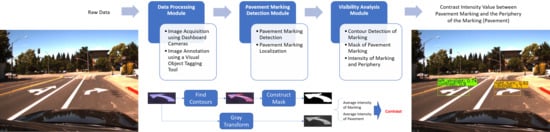
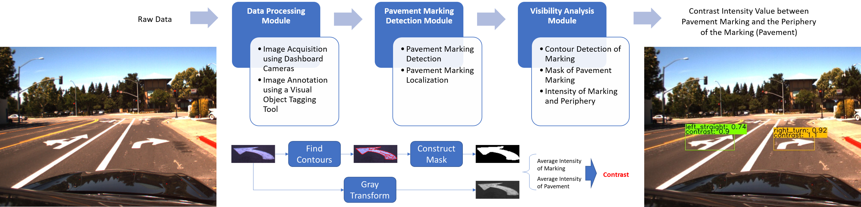
3. Methodology
3.1. Data Processing Module
3.1.1. Data Acquisition
3.1.2. Data Annotation
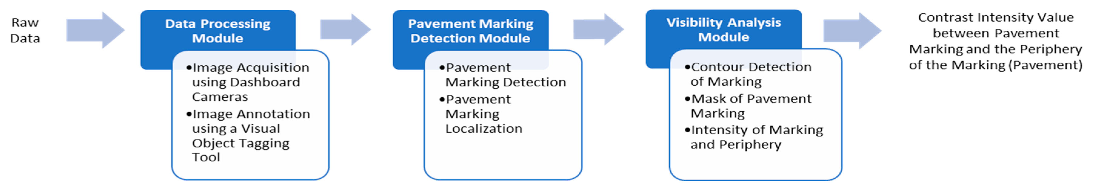
3.2. Pavement Markings Detection Module
3.2.1. Demonstration of the YOLO Framework
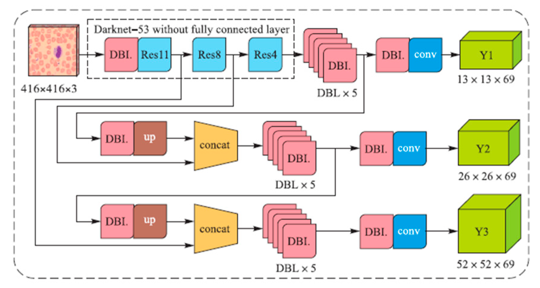
3.2.2. Structure of YOLOv3
3.3. Visibility Analysis Module
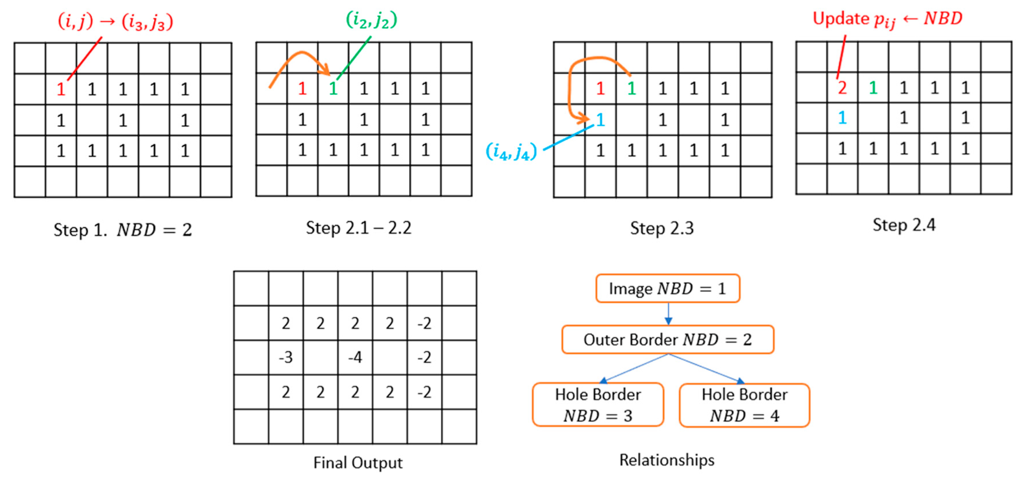
3.3.1. Finding Contours
- Step 1.
- If and , which indicate that this point is the starting point of an outer border, increment by 1 and set . If and , which means it leads a hole border, increment by 1 and set and in case . Otherwise, jump to Step 3.
- Step 2.
- From this starting point , perform the following operations to trace the border.
- 2.1.
- Starting from pixel , traverse the neighborhoods of pixel in a clockwise direction. In this study, the 4-connected case is selected to determine the neighborhoods, which means only the points connected horizontally and vertically are regarded as the neighborhoods. If a non-zero value exists, denote such pixel as . Otherwise, let and jump to Step 3.
- 2.2.
- Assign and .
- 2.3.
- Taking pixel as the center, traverse the neighborhoods in a counterclockwise direction from the next element to find the first non-zero pixel, and assign it as .
- 2.4.
- Update the value according to Step 2.4 in Figure 6.
- 2.5.
- If , update .
- 2.6.
- If and , update .
- 2.7.
- If the current condition satisfies and , which means it goes back to the starting point, jump to Step 3. Otherwise, assign and and return to Sub-step 2.3.
- Step 3.
- If , update . Let and return to Step 1 to process the next pixel. This algorithm stops after the most bottom-right pixel of the input image is processed.
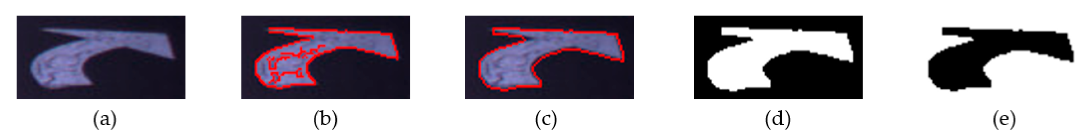
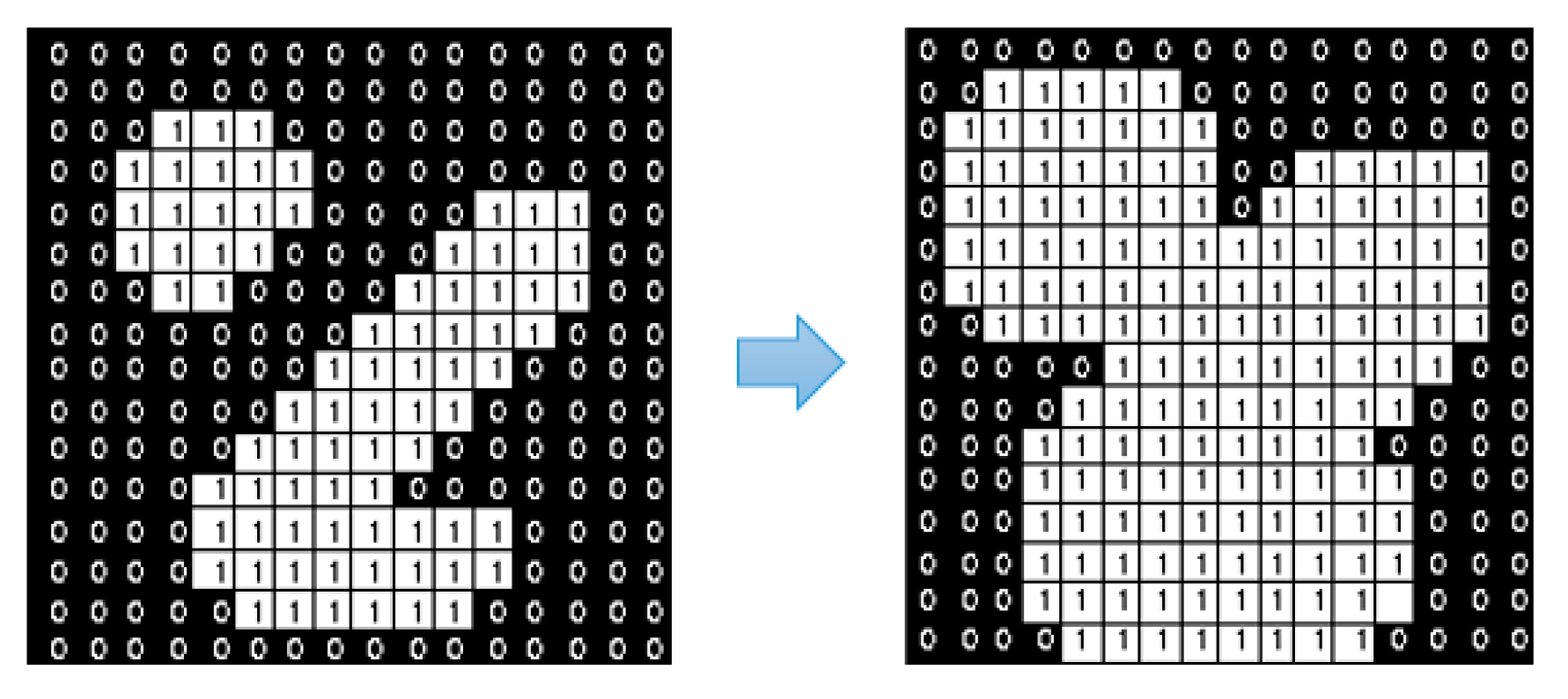
3.3.2. Construct Masks
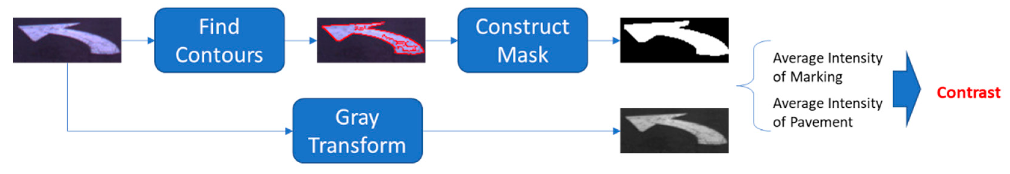
3.3.3. Computing the Intensity Contrast
4. Experimental Validation of the Framework
4.1. Experiment Settings
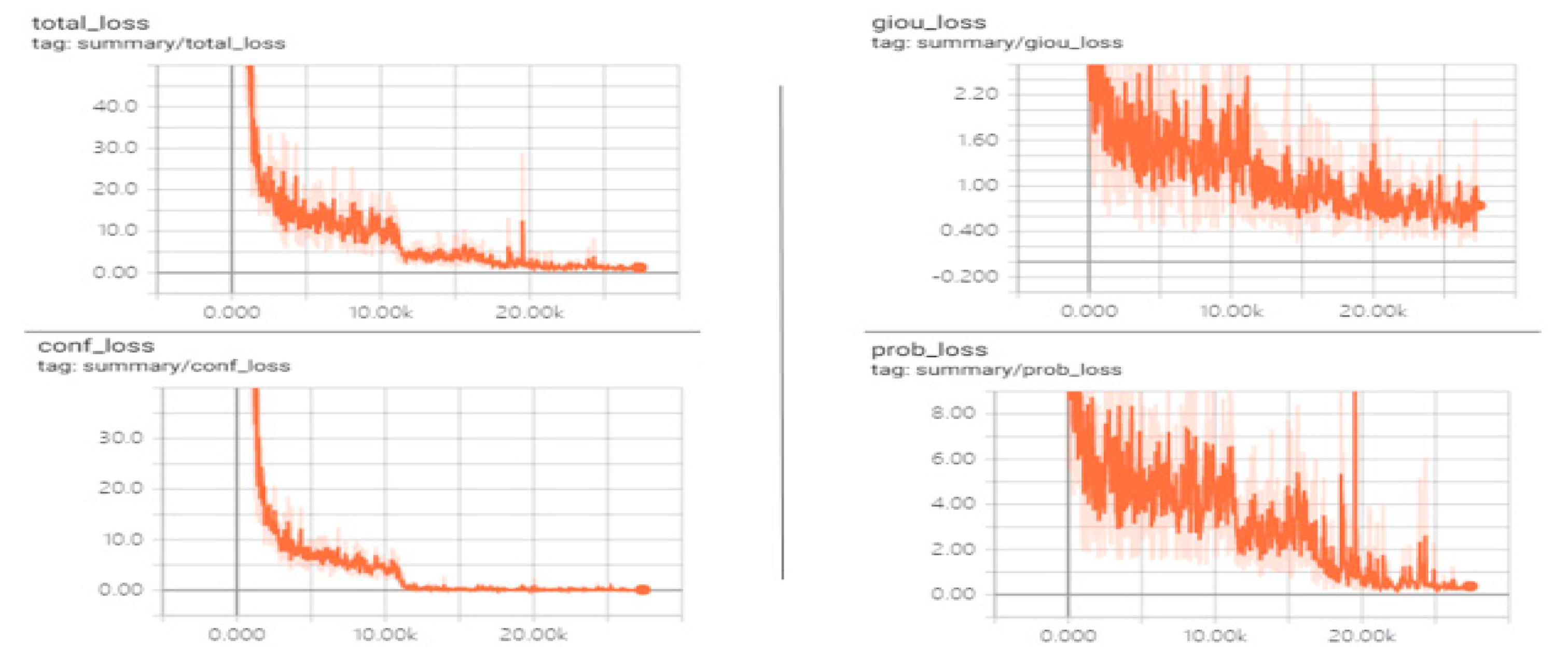
4.2. Model Training
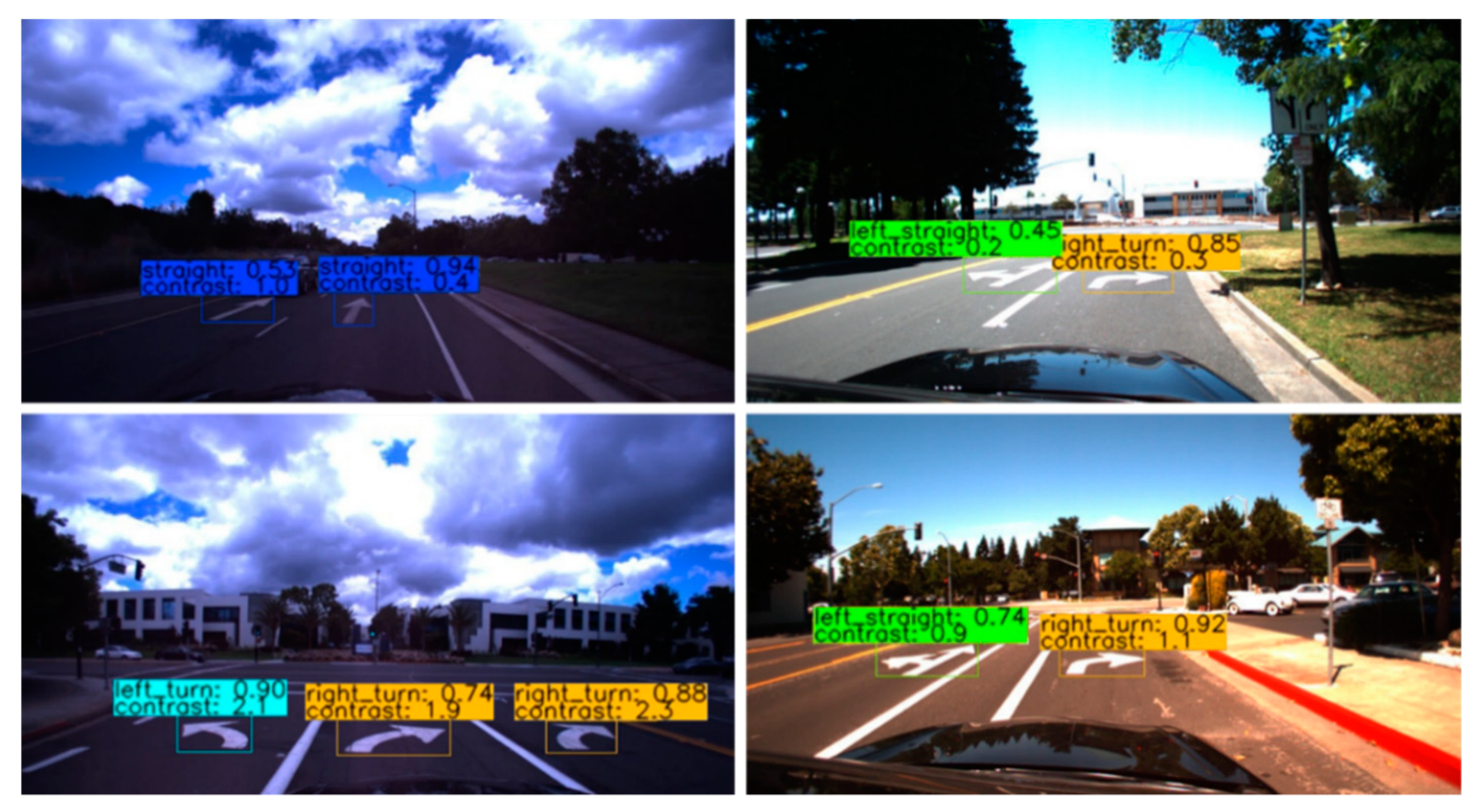
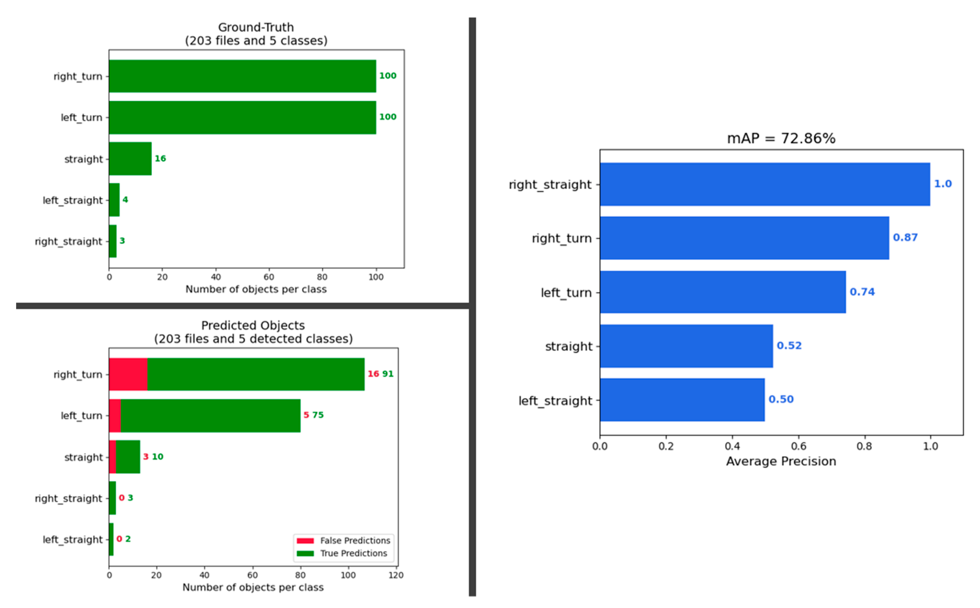
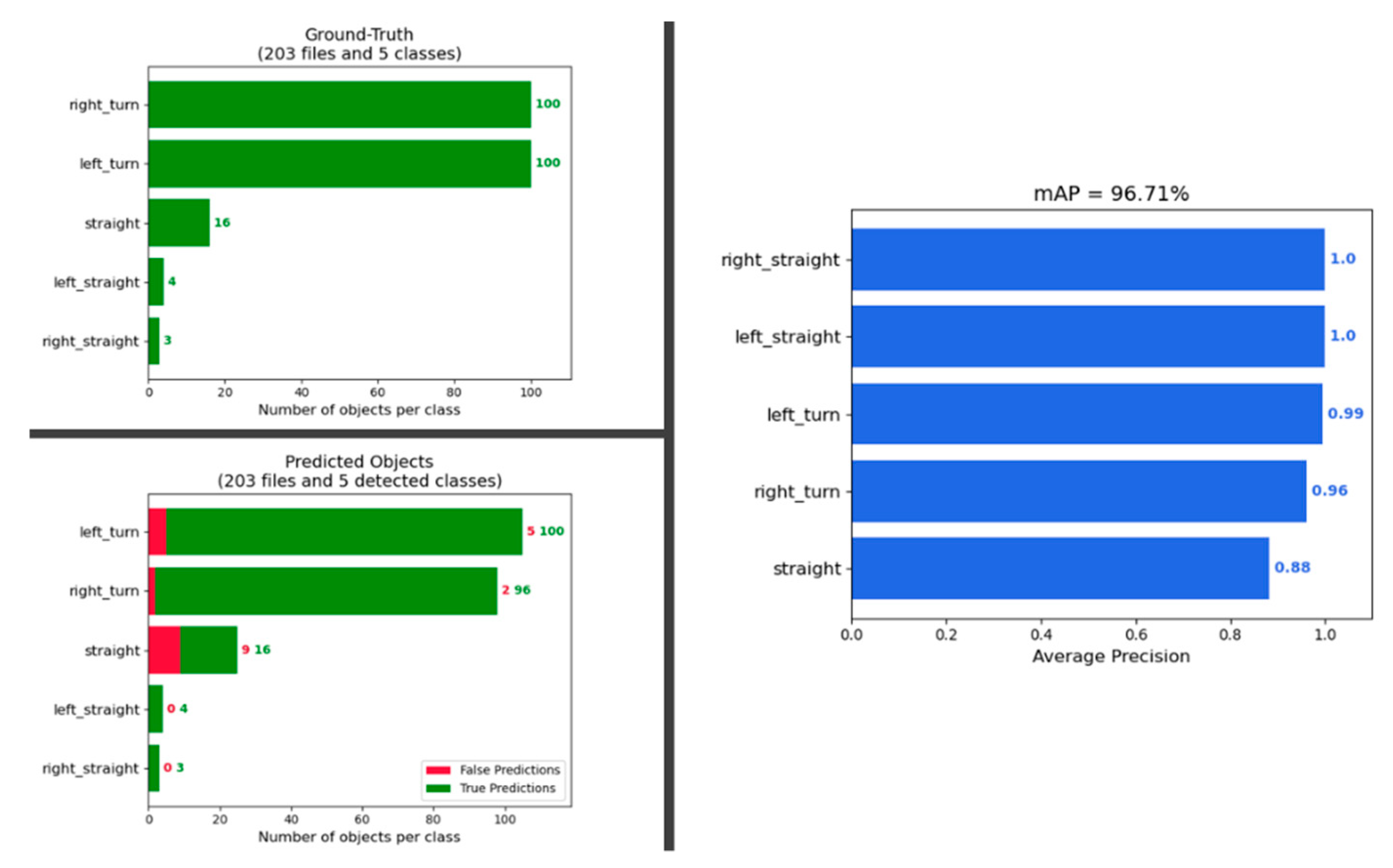
4.3. Model Inference and Performance
5. Conclusions
Author Contributions
Funding
Conflicts of Interest
References
- U.S. Department of Transportation Federal Highway Administration. Available online: https://www.fhwa.dot.gov/policyinformation/statistics/2018/hm15.cfm (accessed on 27 August 2020).
- Ceylan, H.; Bayrak, M.B.; Gopalakrishnan, K. Neural networks applications in pavement engineering: A recent survey. Int. J. Pavement Res. Technol. 2014, 7, 434–444. [Google Scholar]
- El-Basyouny, M.; Jeong, M.G. Prediction of the MEPDG asphalt concrete permanent deformation using closed form solution. Int. J. Pavement Res. Technol. 2014, 7, 397–404. [Google Scholar] [CrossRef]
- Eldin, N.N.; Senouci, A.B. A pavement condition-rating model using backpropagation neural networks. Comput. Aided Civ. Infrastruct. Eng. 1995, 10, 433–441. [Google Scholar] [CrossRef]
- Hamdi; Hadiwardoyo, S.P.; Correia, A.G.; Pereira, P.; Cortez, P. Prediction of Surface Distress Using Neural Networks. In AIP Conference Proceedings; AIP Publishing LLC: College Park, MD, USA, 2017; Volume 1855, p. 040006. [Google Scholar] [CrossRef] [Green Version]
- Li, B.; Wang, K.C.P.; Zhang, A.; Yang, E.; Wang, G. Automatic classification of pavement crack using deep convolutional neural network. Int. J. Pavement Eng. 2020, 21, 457–463. [Google Scholar] [CrossRef]
- Nhat-Duc, H.; Nguyen, Q.L.; Tran, V.D. Automatic recognition of asphalt pavement cracks using metaheuristic optimized edge detection algorithms and convolution neural network. Autom. Constr. 2018, 94, 203–213. [Google Scholar] [CrossRef]
- Xu, G.; Ma, J.; Liu, F.; Niu, X. Automatic Recognition of Pavement Surface Crack Based on B.P. Neural Network. In Proceedings of the 2008 International Conference on Computer and Electrical Engineering, Phuket, Thailand, 20–22 December 2008; pp. 19–22. [Google Scholar] [CrossRef]
- Yamamoto, J.; Karungaru, S.; Terada, K. Road Surface Marking Recognition Using Neural Network. In Proceedings of the 2014 IEEE/SICE International Symposium on System Integration; SII, Tokyo, Janpan, 13–15 December 2014; pp. 484–489. [Google Scholar] [CrossRef]
- Zhang, L.; Yang, F.; Yimin, D.Z.; Zhu, Y.J. Road Crack Detection Using Deep Convolutional Neural Network. In Proceedings of the 2016 IEEE international conference on image processing (ICIP), Phoenix, AZ, USA, 25–28 September 2016; Volume 2016, pp. 3708–3712. [Google Scholar] [CrossRef]
- Meignen, D.; Bernadet, M.; Briand, H. One Application of Neural Networks for Detection of Defects Using Video Data Bases: Identification of Road Distresses. In Proceedings of the International Conference on Database and Expert Systems Applications, 8th International Conference, Toulouse, France, 1–5 September 1997; pp. 459–464. [Google Scholar] [CrossRef]
- Zhang, A.; Wang, K.C.P.; Fei, Y.; Liu, Y.; Chen, C.; Yang, G.; Li, J.Q.; Yang, E.; Qiu, S. Automated pixel-level pavement crack detection on 3D asphalt surfaces with a recurrent neural network. Comput.-Aided Civ. Infrastruct. Eng. 2019, 34, 213–229. [Google Scholar] [CrossRef]
- Chen, T.; Chen, Z.; Shi, Q.; Huang, X. Road marking detection and classification using machine learning algorithms. In Proceedings of the 2015 IEEE Intelligent Vehicles Symposium (IV), Seoul, Korea, 28 June–1 July 2015; Volume 2015, pp. 617–621. [Google Scholar] [CrossRef]
- Gurghian, A.; Koduri, T.; Bailur, S.V.; Carey, K.J.; Murali, V.N. DeepLanes: End-To-End Lane Position Estimation Using Deep Neural Networks. In Proceedings of the 2016 IEEE Computer Society Conference on Computer Vision and Pattern Recognition Workshops, Las Vegas, NV, USA, 26 June–1 July 2016. [Google Scholar] [CrossRef]
- Lee, S.; Kim, J.; Yoon, J.S.; Shin, S.; Bailo, O.; Kim, N.; Lee, T.H.; Hong, H.S.; Han, S.H.; Kweon, I.S. VPGNet: Vanishing Point Guided Network for Lane and Road Marking Detection and Recognition. In Proceedings of the 2017 IEEE International Conference on Computer Vision, Venice, Italy, 22–29 October 2017. [Google Scholar] [CrossRef] [Green Version]
- Geiger, A.; Lenz, P.; Stiller, C.; Urtasun, R. Vision meets robotics: The KITTI dataset. Int. J. Robot. Res. 2013, 32, 1231–1237. [Google Scholar] [CrossRef] [Green Version]
- Griffin, G.; Holub, A.; Perona, P. Caltech-256 object category dataset. Caltech Mimeo 2007, 11. Available online: http://authors.library.caltech.edu/7694 (accessed on 27 August 2020).
- Yu, F.; Chen, H.; Wang, X.; Xian, W.; Chen, Y.; Liu, F.; Madhavan, V.; Darrell, T. BDD100K: A Diverse Driving Dataset for Heterogeneous Multitask Learning. In Proceedings of the 2020 IEEE/CVF Conference on Computer Vision and Pattern Recognition (CVPR), Seattle, WA, USA, 13–19 June 2020. [Google Scholar] [CrossRef]
- GitHub Repository. Available online: https://github.com/microsoft/VoTT (accessed on 27 August 2020).
- Liu, L.; Ouyang, W.; Wang, X.; Fieguth, P.; Chen, J.; Liu, X.; Pietikäinen, M. Deep learning for generic object detection: A survey. Int. J. Comput. Vis. 2020, 128, 261–318. [Google Scholar] [CrossRef] [Green Version]
- Girshick, R.; Donahue, J.; Darrell, T.; Malik, J. Rich Feature Hierarchies for Accurate Object Detection and Semantic Segmentation. In Proceedings of the 2014 IEEE Computer Society Conference on Computer Vision and Pattern Recognition, Columbus, OH, USA, 23–28 June 2014; pp. 580–587. [Google Scholar] [CrossRef] [Green Version]
- Girshick, R. Fast R-CNN. In Proceedings of the 2015 IEEE International Conference on Computer Vision, Santiago, Chile, 7–13 December 2015; pp. 1440–1448. [Google Scholar]
- Ren, S.; He, K.; Girshick, R.; Sun, J. Faster R-CNN: Towards real-time object detection with region proposal networks. IEEE Trans. Pattern Anal. Mach. Intell. 2017, 39, 1137–1149. [Google Scholar] [CrossRef] [PubMed] [Green Version]
- Redmon, J.; Divvala, S.; Girshick, R.; Farhadi, A. You Only Look Once: Unified, Real-Time Object Detection. In Proceedings of the 2016 IEEE Computer Society Conference on Computer Vision and Pattern Recognition, Vegas, NV, USA, 27–30 June 2016; Volume 2016. [Google Scholar] [CrossRef] [Green Version]
- Redmon, J.; Farhadi, A. YOLO9000: Better, Faster, Stronger. Available online: http://pjreddie.com/yolo9000/ (accessed on 23 November 2020).
- Redmon, J.; Farhadi, A. YOLOv3: An Incremental Improvement. Available online: http://arxiv.org/abs/1804.02767 (accessed on 23 November 2020).
- Ioffe, S.; Szegedy, C. Batch Normalization: Accelerating Deep Network Training by Reducing Internal Covariate Shift. In Proceedings of the 32nd International Conference on Machine Learning, Lille, France, 6–11 July 2015; Volume 1, pp. 448–456. Available online: https://arxiv.org/abs/1502.03167v3 (accessed on 23 November 2020).
- Zhong, Y.; Wang, J.; Peng, J.; Zhang, L. Anchor Box Optimization for Object Detection. In Proceedings of the 2020 IEEE Winter Conference on Applications of Computer Vision, Snowmass Village, CO, USA, 1–5 March 2020. [Google Scholar] [CrossRef]
- He, K.; Zhang, X.; Ren, S.; Sun, J. Deep Residual Learning for Image Recognition. In Proceedings of the 2016 IEEE Computer Society Conference on Computer Vision and Pattern Recognition, Vegas, NV, USA, 27–30 June 2016; Volume 2016, pp. 770–778. [Google Scholar] [CrossRef] [Green Version]
- Suzuki, S.; Be, K.A. Topological structural analysis of digitized binary images by border following. Comput. Vis. Graph. Image Process. 1985, 30, 32–46. [Google Scholar] [CrossRef]
- Bradski, G. The OpenCV Library. Dr. Dobbs J. Softw. Tools 2000, 25, 120–125. [Google Scholar] [CrossRef]
- Liang, J.I.; Piper, J.; Tang, J.Y. Erosion and dilation of binary images by arbitrary structuring elements using interval coding. Pattern Recognit. Lett. 1989, 9, 201–209. [Google Scholar] [CrossRef]
- Klein, S.A.; Carney, T.; Barghout-Stein, L.; Tyler, C.W. Seven models of masking. In Human Vision and Electronic Imaging II.; International Society for Optics and Photonics: Bellingham, WA, USA, 1997; Volume 3016, pp. 13–24. [Google Scholar]
- Abadi, M.; Agarwal, A.; Barham, P.; Brevdo, E.; Chen, Z.; Citro, C.; Corrado, G.S.; Davis, A.; Dean, J.; Devin, M.; et al. TensorFlow: Large-Scale Machine Learning on Heterogeneous Distributed Systems; Distributed, Parallel and Cluster Computing. Available online: http://arxiv.org/abs/1603.04467 (accessed on 23 November 2020).
- Longadge, R.; Dongre, S. Class imbalance problem in data mining review. Int. J. Comput. Sci. Netw. 2013, 2. Available online: http://arxiv.org/abs/1305.1707 (accessed on 23 November 2020).
- Pan, S.J.; Yang, Q. A survey on transfer learning. In IEEE Transactions on Knowledge and Data Engineering; IEEE: Piscataway, NJ, USA, 2010; Volume 22, pp. 1345–1359. [Google Scholar] [CrossRef]
- Lin, T.Y.; Maire, M.; Belongie, S.; Hays, J.; Perona, P.; Ramanan, D.; Dollár, P.; Zitnick, C.L. Microsoft COCO: Common objects in context. In European Conference on Computer Vision; Springer: Cham, Switzerland, 2014; 8693 LNCS (PART 5); pp. 740–755. [Google Scholar] [CrossRef] [Green Version]
- Davis, J.; Goadrich, M. The relationship between precision-recall and ROC curves. In ACM International Conference Proceeding Series; ACM: New York, NY, USA, 2006; Volume 148, pp. 233–240. [Google Scholar] [CrossRef] [Green Version]


| Positive Predication | Negative Prediction | |
|---|---|---|
| Positive Label | TP | FN |
| Negative Label | FP | TN |
Publisher’s Note: MDPI stays neutral with regard to jurisdictional claims in published maps and institutional affiliations. |
© 2020 by the authors. Licensee MDPI, Basel, Switzerland. This article is an open access article distributed under the terms and conditions of the Creative Commons Attribution (CC BY) license (http://creativecommons.org/licenses/by/4.0/).
Share and Cite
Kang, K.; Chen, D.; Peng, C.; Koo, D.; Kang, T.; Kim, J. Development of an Automated Visibility Analysis Framework for Pavement Markings Based on the Deep Learning Approach. Remote Sens. 2020, 12, 3837. https://0-doi-org.brum.beds.ac.uk/10.3390/rs12223837
Kang K, Chen D, Peng C, Koo D, Kang T, Kim J. Development of an Automated Visibility Analysis Framework for Pavement Markings Based on the Deep Learning Approach. Remote Sensing. 2020; 12(22):3837. https://0-doi-org.brum.beds.ac.uk/10.3390/rs12223837
Chicago/Turabian StyleKang, Kyubyung, Donghui Chen, Cheng Peng, Dan Koo, Taewook Kang, and Jonghoon Kim. 2020. "Development of an Automated Visibility Analysis Framework for Pavement Markings Based on the Deep Learning Approach" Remote Sensing 12, no. 22: 3837. https://0-doi-org.brum.beds.ac.uk/10.3390/rs12223837