An Analytical Framework for Accurate Traffic Flow Parameter Calculation from UAV Aerial Videos


1
Chair of Geoinformatics, Faculty of Geodesy, University of Zagreb, Kačićeva 26, 10000 Zagreb, Croatia
2
Department of Transport Planning, Faculty of Transport and Traffic Sciences, University of Zagreb, Vukelićeva 4, 10000 Zagreb, Croatia
*
Author to whom correspondence should be addressed.
Remote Sens. 2020, 12(22), 3844; https://0-doi-org.brum.beds.ac.uk/10.3390/rs12223844
Submission received: 25 September 2020
/
Revised: 19 November 2020
/
Accepted: 21 November 2020
/
Published: 23 November 2020
(This article belongs to the Special Issue Traffic Assessment and Monitoring with Remote Sensing and Geospatial Modelling)
Abstract
:Unmanned Aerial Vehicles (UAVs) represent easy, affordable, and simple solutions for many tasks, including the collection of traffic data. The main aim of this study is to propose a new, low-cost framework for the determination of highly accurate traffic flow parameters. The proposed framework consists of four segments: terrain survey, image processing, vehicle detection, and collection of traffic flow parameters. The testing phase of the framework was done on the Zagreb bypass motorway. A significant part of this study is the integration of the state-of-the-art pre-trained Faster Region-based Convolutional Neural Network (Faster R-CNN) for vehicle detection. Moreover, the study includes detailed explanations about vehicle speed estimation based on the calculation of the Mean Absolute Percentage Error (MAPE). Faster R-CNN was pre-trained on Common Objects in COntext (COCO) images dataset, fine-tuned on 160 images, and tested on 40 images. A dual-frequency Global Navigation Satellite System (GNSS) receiver was used for the determination of spatial resolution. This approach to data collection enables extraction of trajectories for an individual vehicle, which consequently provides a method for microscopic traffic flow parameters in detail analysis. As an example, the trajectories of two vehicles were extracted and the comparison of the driver’s behavior was given by speed—time, speed—space, and space—time diagrams.
1. Introduction
The number of vehicles in Europe is increasing every year. According to the European Automobile Manufacturers Association (ACEA), in 2019, there were 531 passenger cars per 1000 inhabitants in the European Union (EU). Comparing this number with 497 cars in 2014, it gives a 7% increase over five years [1]. This amount of growth in the number of vehicles requires new solutions in the transport infrastructure. Numerical values describing each road are indispensable and essential for performing a proper analysis. This is the main task of traffic engineers, who usually describe the flow using deterministic modeling of traffic flow parameters, depending on their requirements. These parameters can be divided into two groups: macroscopic and microscopic. According to Rao, the macroscopic parameters characterize the traffic as a whole and microscopic parameters study the behavior of an individual vehicle in the flow relating to one another [2]. Parameters, such as the traffic flow rate, speed, and density are three fundamental macroscopic traffic flow parameters that are used to describe the state of continuous traffic flow [2]. Microscopic parameters are gross and net time headways (time headways and time gaps), and gross and net distance headways (distance headways and distance gaps) [3]. Collecting accurate and detailed traffic flow data and obtaining parameters at specific locations can be a very expensive, demanding, and time-consuming process. It often involves significant man-hours and expensive technologies that have limitations in collecting all the necessary data. These include traffic data acquisition techniques, such as pneumatic road tubes, induction loops, video image detection, piezoelectric sensors, and smartphone applications with their advantages and disadvantages [4,5,6]. However, contrary to the above techniques, Unmanned Aerial Vehicles (UAVs) represent more efficient and simpler solutions for many tasks, including the collection of traffic data [7]. The Single European Sky Air Traffic Management (ATM) Research Joint Undertaking (SESAR JU), established by the European Union Council provided a projection that more than seven million consumer leisure UAVs will operate across Europe by 2050 [8]. According to SESAR JU, one of the reasons for the large growth in the number of commercial and government UAVs is their capability to collect data from aerial points that had been inaccessible in the past. Besides, the European Union is currently investing 40 million euros through the SESAR JU project to integrate UAVs into the controlled airspace, indicating serious EU plans for UAV usage.
The main aim of this study is to propose a new framework for low-cost, location-specific traffic flow parameter measurements for the calibration of the deterministic traffic flow models. To provide a basis for deciding on new solutions, a detailed analysis of the current situation was required. For this reason, the proposed framework had the purpose of consolidating all of the procedures needed to collect highly accurate traffic flow parameter values (flow, density, speed, headway, gap, etc.); from terrain operations, through image processing, vehicle detection and tracking to traffic flow parameters estimation. Moreover, the proposed framework included spatial analyses that are significant for obtaining microscopic traffic flow parameters. Since decisions about the reconstruction of the existing and the construction of new roads are time-consuming processes, it is not necessary to derive traffic flow parameters in real time. In this paper, the emphasis is on achieving high accuracy in parameter determination. For this reason, a robust state-of-the-art object detection method was integrated into the framework. It is a significant part of the study, and the results of using the stated method are supported by the evaluation metrics. Except for standard evaluation metrics of object detection methods, the displacement of the detected and ground truth vehicles is also provided in this paper.
This paper is organized as follows: after a brief introduction to the research topic and a brief overview of the related papers, the sections on data collection and methods explain in detail the parts of the proposed framework. For ease of reading and understanding, the framework is divided into four segments: terrain survey, image processing, object detection, and parameters estimation. This is followed by a section in which the results of the performed analyses are presented in the form of tables and diagrams. Moreover, the results section gives an insight into the evaluation of metric values for the proposed framework. This is followed by a proper discussion of the given results and the advantages and disadvantages of the proposed framework given the currently developed methods presented in the related papers. Finally, according to the results and outcome of the discussion, a brief conclusion is provided with future research options for traffic data collection.
Related Works
For the reasons mentioned above, it is evident that more and more research projects are currently relying on the use of UAVs. Many scientific articles in traffic science refer to the use of UAVs for real-time traffic monitoring and management [7,9,10,11,12]. Unlike real-time traffic monitoring and management, the collection of traffic data from UAVs is the subject of research in several papers. Khan et al., used UAVs to estimate the traffic flow parameters and to automatically identify the flow state and the shockwaves at the signaled intersections [13]. To achieve the above goals, a UAV was hovered above the road intersection on an eccentric position regarding the intersection center. For vehicle detection, Khan et al., used computer vision techniques such as optical flow, background subtraction, and blob analysis. In terms of traffic flow parameters, all macroscopic parameters (traffic flow rate, speed, density) and one microscopic parameter (net distance headways) were derived. On the evaluation metrics side, the authors provided the evaluation metrics of speed estimation for a single vehicle. In another study, Ke et al., created a UAV-based framework for real-time traffic flow parameter estimation [14]. Their framework consisted of vehicle detection and parameter estimation. For vehicle detection, they used the Haar cascade and a Convolutional Neural Network (CNN) as an ensemble classifier and optical flow. In terms of traffic flow parameters, they also derived macroscopic parameters (traffic flow rate, speed, and density), while the microscopic parameters estimation was not performed within this study. The training process was performed on 18,000 images, while testing was performed on 2000 images. Similar study was made by Chen et al. where the authors proposed a four-step framework with the aim to extract vehicle trajectories from a UAV-based video. Vehicle detection segment was performed by ensemble Canny-based edge detector, while the tracking process is based on Kernelized Correlation Filter (KCF) algorithm. Particular emphasis is on the conversion image Cartesian coordinates to Frenet coordinates and on smoothing vehicle trajectories constructed from Frenet coordinates [15].
Apart from the aforementioned papers aimed at collecting traffic flow data from UAVs with a precise vehicle detection method, few works have been focused explicitly on detecting vehicles or collecting traffic data from a fixed camera. Fedorov et al. applied a fine-tuned object detection network to estimate the traffic flow from a surveillance camera [16]. They used a fine-tuned Mask Region-based Convolution Neural Network (Mask R-CNN) for vehicle detection in six classes: car, van, truck, tram, bus, and trolleybus. They also provided a comparison of manually collected traffic flow rate and traffic flow rate based on their object detection network for the observed road intersection. A surveillance camera was placed high above the road intersection. In terms of traffic flow parameters, only the macroscopic parameters were presented. The fine-tuning process was performed by 786 images, while 196 images were used for evaluation. On the other hand, Wang et al., focused on detecting vehicles from UAV [17]. They developed a vehicle detecting and tracking system based on the optical flow. They also explained in detail four segments of the system: image registration, image features extraction, vehicle shape detection, and vehicle tracking. As previously listed studies, the computation of microscopic parameters was not performed in this study.
2. Data Collections and Methods
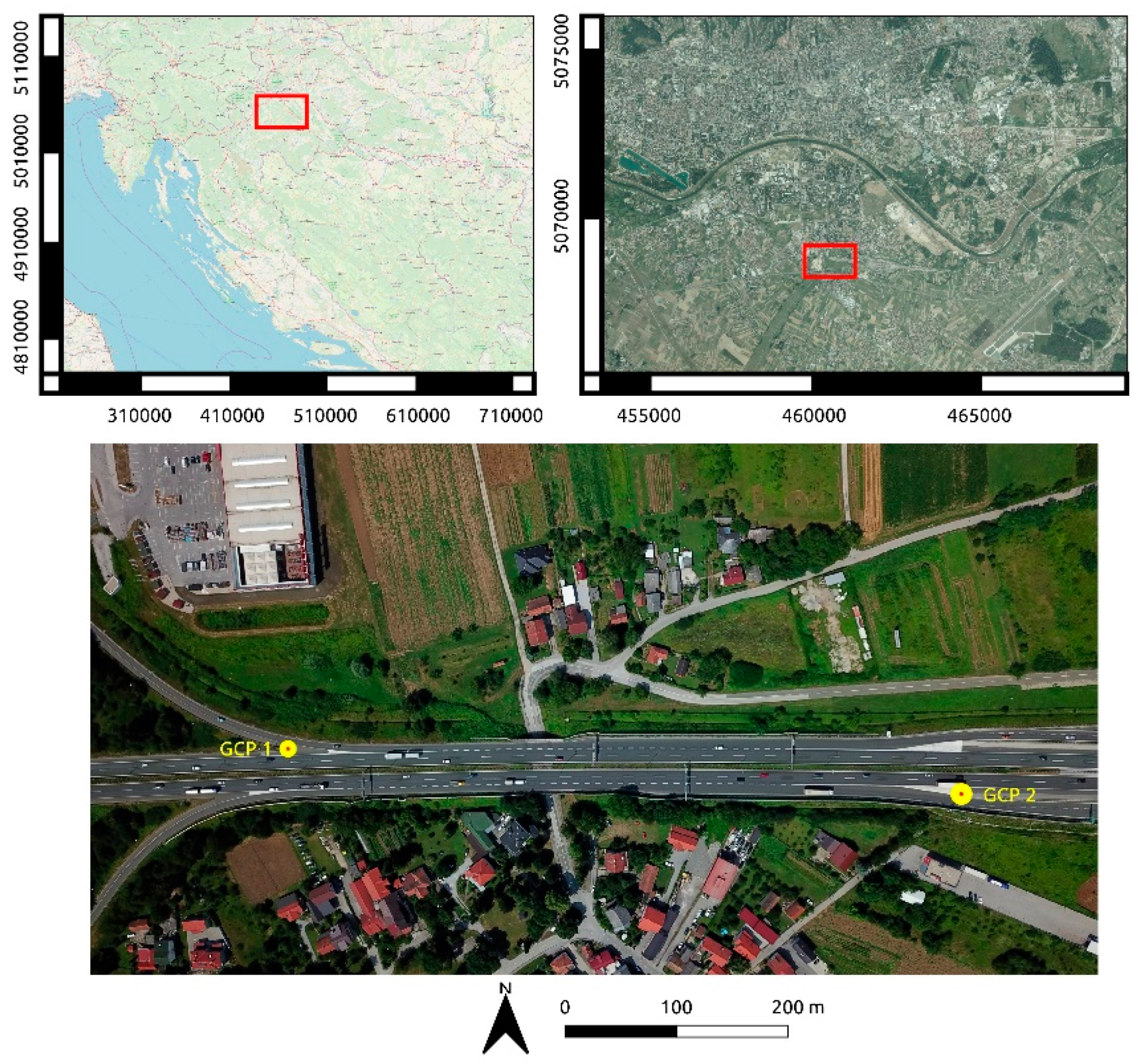
The motorization rate in the City of Zagreb in 2011 was 408 passenger cars per 1000 inhabitants [18]. The Zagreb bypass is the busiest motorway in Croatia with the traffic rate continuously rising [18]. The location of this research is an approximately 500 m long section of Zagreb bypass motorway (Figure 1). It is a part of the A3 national highway, and it extends in the northwest–southeast direction. The specified section of the road consists of two lanes with entries and exits in both directions. Figure 1 shows the study area on the Open Street Map (OSM) and the Croatian digital orthophoto with Ground Control Points (GCPs) marked on the image from UAV. The research area was observed between 4:00 p.m. and 4:15 p.m. assuming this is the time of increased traffic density because of the migration of workers after a working day, which is usually between 8:00 a.m. and 4:00 p.m. in Croatia. Moreover, according to the Highway Capacity Manual, a period of 15 min is considered to be a representative period for traffic analysis during the peak hour [19]. Increased traffic density presents ideal conditions for testing the proposed framework, with particular emphasis on vehicle detection and describing the traffic flow by suitable parameters.
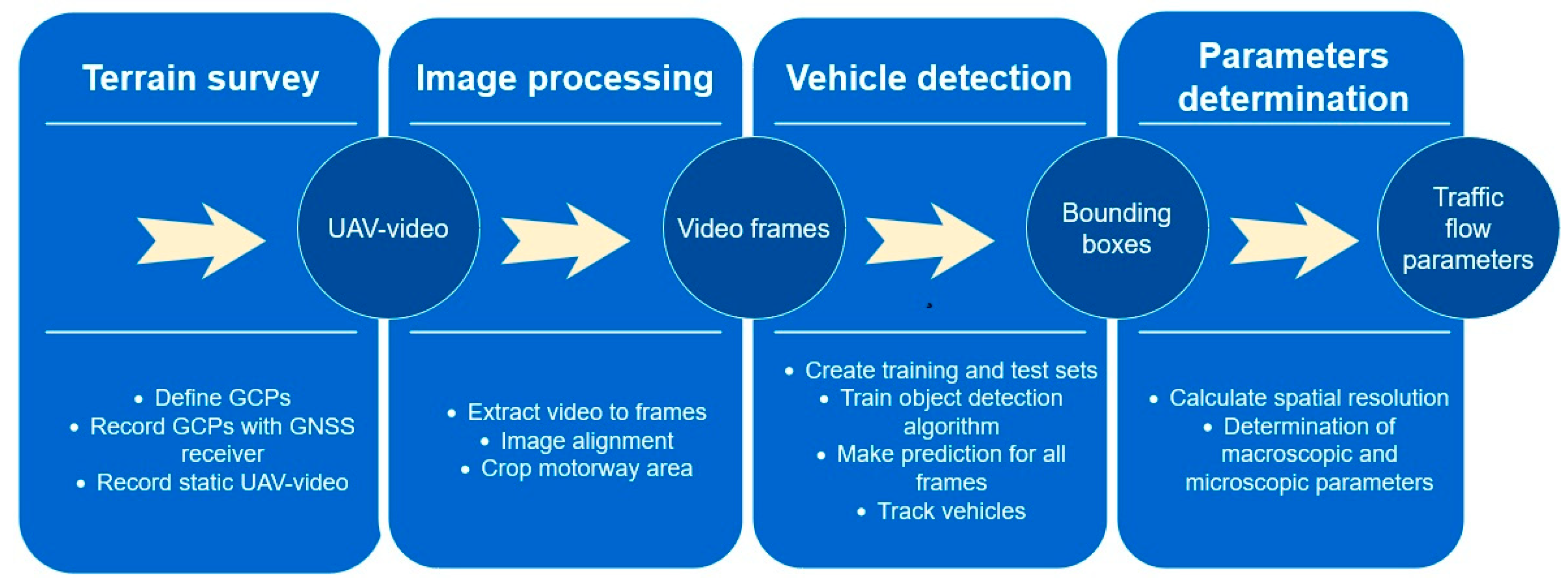
The proposed framework for collecting traffic data and obtaining traffic flow parameters consists of four segments: terrain survey, image processing, vehicle detection, and determination of traffic flow parameters. All of the above segments contain sub-segments, which will be explained in detail below (Figure 2).
2.1. Terrain Survey
The terrain survey segment includes defining two Ground Control Points (GCPs), determination of their positions, and recording a UAV-video of the observed area. GCPs are defined with unique terrain points: GCP1 on the edge of a road fence, while GCP2 was defined as the intersection of two white lanes (Figure 1). Considering that in this paper GCPs are used to determine the spatial resolution with high accuracy, which is a two-dimensional problem, the usage of the two GCPs is sufficient for this task. The positions of GCPs were recorded in the Croatian reference coordinate system with dual-frequency Global Navigation Satellite System (GNSS) Topcon HiPer Site Reciver (SR) obtaining GNSS corrections from the state network of referential GNSS stations - Croatian Positioning System (CROPOS). This is a very important part of the study for calculating the spatial resolution of images, which is a key detail for the determination of the traffic flow parameters. Considering that parameters such as density, speed, and distance headways are based on spatial distances, the accuracy of the mentioned parameters is directly connected with spatial resolution. After that, the observation area was recorded for approximately 14 min with a UAV. The UAV was nearly static and stabilized by an onboard GNSS. Moreover, the UAV was positioned vertically to enable a more accurate estimation of car positions. The flight height was near 50 m. The UAV was exposed to a light wind and the recorded video was not entirely stable.
2.2. Image Processing
The image-processing segment includes extracting frames from the UAV-video, image alignment, and cropping the motorway area. OpenCV library in Python programming language was used to make this segment. There was a 13:52 min long video, which was extracted to 19,972 frames that match the UAV frame rate of 24 fps (24 Hz). Since the video was not perfectly stable, image (frame) alignment had to be applied. Image alignment consists of applying feature descriptors to images and finding homography between images. Awad and Hassaballah described most of the existing feature detectors concisely in their book [20]. According to Pieropan et al. Oriented Features from accelerated segment test (FAST) and Rotated (ORB) and Binary Robust Invariant Scalable Keypoints (BRISK) have the best performance with motion blur videos; therefore, ORB was used in this study [21]. As its name suggests, ORB is a very fast binary descriptor which relies on Binary Robust Independent Elementary Features (BRIEF), where BRIEF is rotation invariant and resistant to noise [22]. Apart from the feature descriptors, homography is also the main part of the image alignment. Homography is a transformation that maps the points from one image to the corresponding points in the other image [23]. Moreover, feature descriptors usually do not perform perfectly, so to calculate homography, a robust estimation technique must be used [24]. For this purpose, the OpenCV algorithm using the Random Sample Consensus (RANSAC) technique was used, which Fischler and Bolles explained in detail [25]. Unlike traditional sampling techniques, which are based on a large set of data points, RANSAC is a resampling technique, which generates candidate solutions by using the minimum number observations (data points) required to estimate the underlying model parameters. Ma et al., presented more about homography [26]. In this study all frames were aligned with the first frame, which is better known as a master–slave technique, where the first frame is characterized as the master image, and all of the other frames as slaves [27].
Finally, the last step in the image-processing segment was cropping images around the motorway. The original video was recorded in 4096 × 2160 pixels dimension, which required a lot of memory while being processed. This amount of memory utilization can slow down the processing of the object detection. Depending on the hardware resources, with such high memory requirements, the algorithm may not even be able to complete the calculations. Therefore, frames must be cropped to the observation area only, i.e., a narrow area along the motorway. After cropping, the individual frame dimensions were 3797 × 400 pixels (Figure 3). Finally, the images were ready for the vehicle detection segment.
2.3. Vehicle Detection
This is computationally the most resource-intensive segment of the study. An Intel Core 2 Quad Central Processing Unit (CPU) with 256 GB RAM and 2 NVIDIA GP104GL Quadro P4000, 8 GB GDDR5 memory Graphical Processing Units (GPUs) was used. The deep learning part of this segment was done with a TensorFlow object detection application programming interface (API).
In this study, deep learning object detection was applied for vehicle detection. There are many object detection methods based on deep learning [28]. All of them can be divided into two-stage and one-stage detectors [29]. Two-stage detectors firstly obtain a significant number of regions of interest (ROI), usually with Region Proposal Network (RPN) or Features Pyramid Network (FPN), and then use CNN to evaluate every ROI [30]. Unlike two-stage detectors, one-stage detectors suggest ROI directly from the image, without using any region proposal technique, which is time-efficient and can be used for real-time applications [29]. Because of their complexity two-stage detectors have an advantage in accuracy [31]. Since this study is not based on real-time tracking and vehicles are very small on the images, a two-stage detector was used. According to the results of the research made by Liu et al., and the availability of the mentioned hardware, Faster R-CNN with ResNet50 backbone network, pre-trained on the COCO images dataset, was selected as an optimal network for this study [32,33]. Faster R-CNN detector is described in detail by Ren et al. [34]. Since Faster R-CNN was pre-trained, this process of training is called transfer learning. It enables training with a small dataset of images, and it is a short-time process. A very important part of the Faster R-CNN detector is the selection of anchor’s dimensions, aspect ratios, scales, height, and width strides. All of these parameters are explained in detail by Wang et al. [35]. Targeted selection of these parameters can greatly improve the detection time and accuracy. The height and width of anchors were defined by parameters of ResNet50 CNN, which is explained in detail by He et al. [36]. After analyzing the labeled vehicle sizes and shapes, the parameters presented in Table 1 were used.
Regarding the training and test set of images, 200 images, equally distributed all over the frames, were selected. Selected images were divided into training and test dataset at a ratio of 80:20, i.e., train dataset containing 160 images (4367 vehicles) and test dataset with 40 images (1086 vehicles). According to a very small set of data with unequal distribution of vehicle types, where there are mostly passenger cars with several trucks, buses, and motorcycles, all images were marked by only one class (vehicle). Labeling of vehicles in training and test images was performed by the LabelImg software.
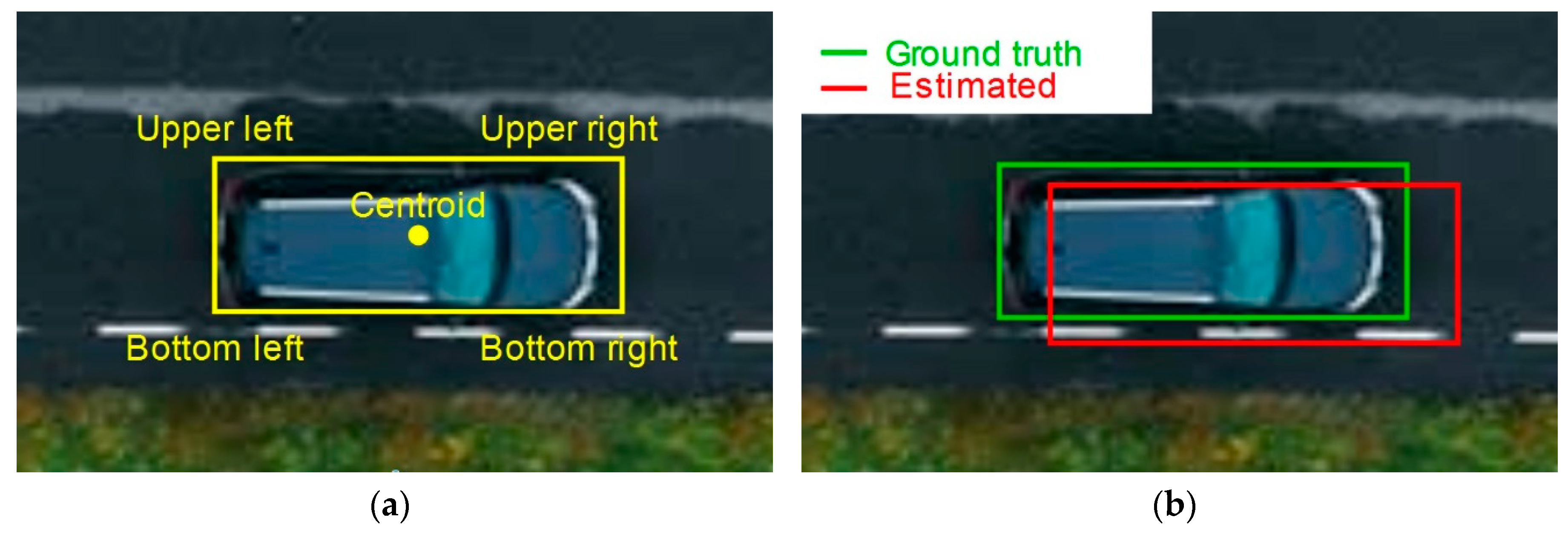
After labeling the vehicles, training started by using the hardware as mentioned above. The training time was 2 h and 35 min and it ended in 22,400 training steps, i.e., 140 training epochs with a batch size of 1. Minimal batch size was selected because of computation resources limitation. Afterward, the trained model was evaluated on a test set of images. From 40 test images, all of 1086 vehicles were manually labeled. For the evaluation process, the confusion matrix was used. The confusion matrix consists of two columns, which represent the numbers of true and false actual vehicles, and two rows, which represent numbers of positive and negative predicted vehicles. Other evaluation metric values, such as precision, recall, accuracy, and F1 score were derived from the confusion matrix. The process of derivation is described in detail by Mohammad and Md Nasair [37]. Finally, a trained model was applied for the prediction of vehicles on all of the frames. The prediction process resulted in frame ID, vehicle ID, confidence score, and coordinates of bounding boxes and centroids of every single detected vehicle. In this study, the bounding boxes analysis was applied to choose the best characterizing point of bounding box for tracking and determining the macroscopic traffic flow parameters. The upper left, upper right, bottom right, bottom left, and centroid points have been considered for this purpose (Figure 4a). The specified characteristic points of the estimated bounding boxes were compared with the same points of ground truth bounding boxes in the test dataset (Figure 4b).
Displacements of specified points were calculated as Root Mean Square Error (RMSE), which is defined by the U.S. Federal Geographical Data Committee as a positional accuracy metric [38]. RMSE values were calculated for all the considered characteristic points with the following equation:
where n is the number of bounding boxes in the test dataset, (xi, yi) are characteristic point coordinates of ground truth bounding boxes, while (xi, yi) are characteristic point coordinates of estimated bounding boxes. Based on RMSE values, the centroid point was selected for tracking and determination of macroscopic parameters.
In terms of microscopic parameters (which will be explained in Section 2.4.2), it is not sufficient to represent a vehicle with one point, not even by a centroid, but it is necessary to use a whole bounding box. The dimensions of the bounding boxes and their location on the image have great impact on the microscopic parameters. To evaluate the detection process of the bounding boxes, the Intersection over Union (IoU) metric was used. IoU is defined with the following equation:
where E is the estimated bounding box, while T is the ground truth bounding box. In this paper, IoU was calculated for every single vehicle and the detection process is evaluated by the mean value of IoU. Mean IoU with already described RMSE values of the characteristic point give adequate metric for microscopic parameters reliability estimation.
Finally, it is necessary to connect the same vehicles between frames by the vehicle ID number. This is done with Simple Online and Realtime Tracking (SORT) algorithm. The algorithm is based on the Kalman filter framework for determining the vehicle speed and IoU parameter between vehicles in two consecutive frames. Bewley et al. provided more details about the SORT algorithm [39]. By applying the SORT algorithm for tracking vehicles, the object detection segment is finished, and the output of this segment is also the input for the last one, i.e., the segment for parameter determination.
2.4. Parameters Determination
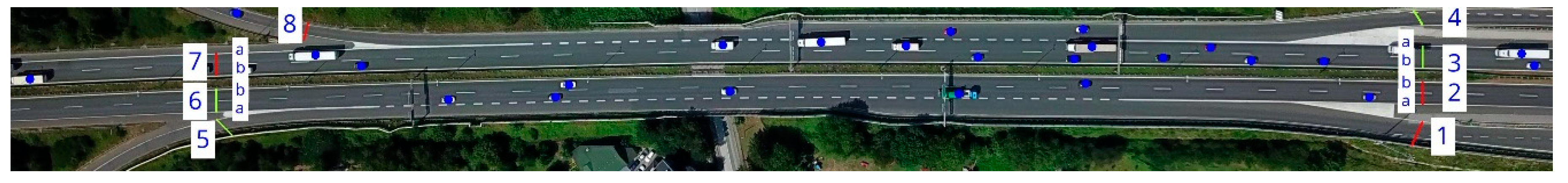
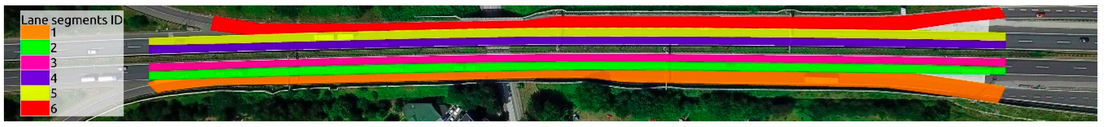
The last part of this study is closely related to traffic flow parameters measurement and calculation. As already stated, one of the aims of this study is to collect the traffic flow data and measure and calculate the traffic flow parameters. Considering this, the traffic flow parameters were measured at the beginning and at the end of the observed road section for individual through lanes on the motorway and on the entry and exit slip lanes. The location-based parameters such as traffic flow rate, time mean speed and time headways and gaps were determined at the characteristic locations of the observed area. That makes a total of 12 locations, marked with numbers from 1 to 8, which is shown in Figure 5. For locations 2, 3, 6 and 7 there are separate lanes a and b, where a lanes represent a slower track and b lanes a faster track. Contrary to location-based parameters, segment-based parameters such as space mean speed, traffic flow density, and distance headways and gaps were determined for each lane segment, which is shown in Figure 6. Each lane segment is approximately 386 m long and marked with numbers from 1 to 6.
Since the output of the vehicle detection segment are the coordinates of vehicles bounding boxes and centroids, it allows creating geometry objects such as points for centroids and polygons for bounding boxes. Furthermore, spatial objects allow for spatial analysis, which has been used to estimate the traffic flow parameters. Considering that every lane can be observed as a spatial object, this is the key step for estimating the parameters of each lane. The GeoPandas Python library was used to accomplish these goals. More about spatial operations and GeoPandas can be found in Jordahl [40].
2.4.1. Macroscopic Traffic Flow Parameters
The first of the macroscopic traffic flow parameters is the traffic flow rate. It is defined as the number of vehicles that cross the observed section of the motorway within the specified time interval [41]. The traffic flow rate is usually expressed by the number of vehicles per hour. Since the vehicles were considered as spatial objects, the traffic flow rate was measured with simple spatial operations. This is accomplished by placing a line perpendicular to the track and counting each time the centroid of the vehicle crosses the line.
Observing the flow of traffic with a UAV allows determining the position and speed of each vehicle in each frame. Vehicle positions are defined by vehicle centroids. Based on the centroid coordinates and the given frame rate, the speed of each individual vehicle can be determined by the equation:
where vn is the speed point of an individual vehicle expressed in pixels per frame, dn represents the distance the vehicle has traveled between the two observed frames and N represents the number of consecutive frames between the two observed frames (frame interval).
Since vehicle centroids are not fixed to a single vehicle point but vary from frame to frame, what is presented by RMSE value, determining vehicle speeds for successive frames (N = 1) will result with noisy data. Contrary to consecutive frames, determining the vehicle speeds with large frame intervals will result in a too smooth speed curve, which will lose significant data. In order to define the optimum N, the positions of the one vehicle, sample 139, was manually labeled in each frame. Vehicle 139 was chosen because of its relatively constant speed during its travel through the observation area. The collected data were used as ground truth data in Mean Absolute Percentage Error (MAPE) calculation. The MAPE was calculated between the speed of the truth point on the ground of one example (vehicle 139) and the estimated speed of the same vehicle for each N in the range from 1 to 30. The following equation was used to calculate MAPE:
where represents the ground truth speed in i-th frame; n represents the number of frames; while vi represents the estimated speed in the same frame of vehicle 139.
Based on the calculated MAPE values, N is set to 12, representing a time interval of 0.5 s (24 frames per second / 12 frames = 0.5 s). A particular N was used to estimate the speed of all vehicles in the video. The process of estimating the traffic flow speed can be calculated in two ways: speed at the point of the road (Time Mean Speed (TMS)) or at the moment (Space Mean Speed (SMS)) [3]. The TMS is the average speed of all vehicles crossing the observation spot in a predefined time interval [42]. Contrary to TMS, SMS is defined by spatial weighting given instead of temporal [42]. According to [43], the TMS is connected to a single point in the observed motorway area, while the SMS is connected to a specific motorway segment length. According to [44], SMS is always more reliable than TMS. More about TMS and SMS can be found in [42] and [43]. In this paper, TMS is calculated for 12 characteristic locations of the observed motorway area, while SMS is calculated for each segment of the motorway lanes. Considering that vehicle speeds and their positions are available for each video, SMS was calculated using the following equation:
where m is the number of vehicles, n is the number of frames and vij is the speed of an individual vehicle in a single frame.
The traffic flow density is defined as the number of vehicles on the road per unit distance. For computing traffic flow density, the spatial resolution of images must be determined. Based on the coordinates of the two GCPs and the number of pixels between the two GCPs, the spatial resolution can be calculated with three simple equations:
where d is the spatial distance between GCPs expressed in meters; (x1, y1) are the spatial coordinates of GCP 1; x2 and y2 are the spatial coordinates of GCP 2; n is the image distance between GCPs expressed in pixels; (nx1, ny1) are the coordinates of GCP 1 image; (nx2, ny2) are the coordinates of GCP 2 image and r is the spatial resolution of the images expressed in meters.
The traffic flow density is spatially related to the traffic section and temporally related to the current state. It is usually expressed by the number of vehicles per kilometer [45]. In this study, the traffic flow density is determined for every video frame, but given the amount of data, this paper only shows the average density for each segment of the lane.
2.4.2. Microscopic Traffic Flow Parameters
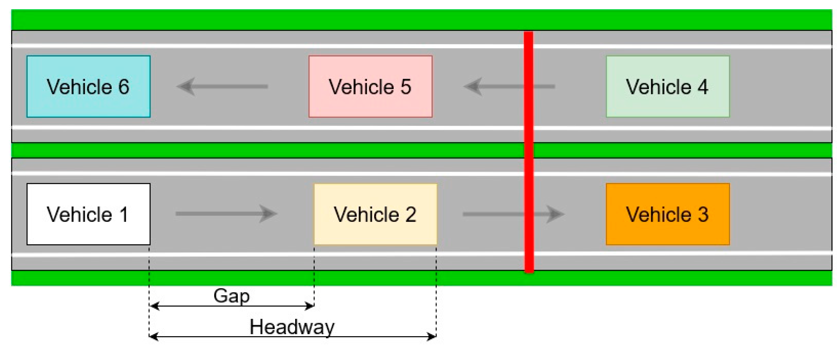
In contrast to macroscopic traffic flow parameters, microscopic parameters consider the interaction of individual vehicles. There are four microscopic parameters: distance headways and gaps, and time headways and gaps. Time headway is defined as the time interval from the front bumper of one vehicle to the front bumper of the next vehicle expressed in one-second unit, while distance headway is the distance between the same points of the vehicles. Opposite to the headways, time gap is defined as the time interval from the back bumper of one vehicle to the front bumper of the next vehicle, also expressed in one-second unit, while distance gap is the distance between the same points of the vehicles [46]. It is important to recognize that the headways are defined between the same points on two consecutive vehicles. Therefore, in this study, headways were calculated between centroids of the vehicle bounding boxes.
Given the coordinates of vehicle bounding boxes and video frame rates are known, and the frames have successive numeric IDs, it is easy to determine the time headways and gaps. Time headway between two vehicles is computed as the difference between the frame ID when the upper right point of the first vehicle crosses the reference line and the frame ID when the upper right point of the next vehicle also crosses the same line. The upper right characteristic point of the vehicle bounding box was selected based on the already described calculation of RMSE values. Then, the calculated number of frames is divided by the frame rate of the video. The time gap between two consecutive vehicles is calculated in a similar way as the time headway with one significant difference: instead of centroids, the characteristic points of the bounding box edges were used to calculate the number of frames. Considering the calculated RMSE values for all characteristic points of the bounding boxes, in this paper the upper left and upper right characteristic points were used to determine the time gap. Therefore, the accuracy of the time gap depends on the positional accuracy of the upper left and upper right points. From the specified definitions of time headways and gaps, the time gap cannot be larger than the time headway, and this can be a good control point when calculating time headways and gaps.
Contrary to time headways and gaps, which are location-based parameters, distance headways, and gaps are segment-based parameters. The distance headways and gaps are calculated for each single frame using spatial resolution. As with the calculation of time headways and gaps, the upper right characteristic points were used for distance headway calculation, while edges of the bounding boxes were used to calculate the distance gaps. Moreover, as in the case of time gaps, the characteristic upper left and upper right points were used, and the accuracy of the distance gaps depends on the positional accuracy of the used characteristic points. Figure 7 shows the difference between headways and gaps, and the reference line for measuring time headways and gaps. From Figure 7, it is clear that the difference between the distance headway and gap represents the length of the observed vehicle. Likewise, as with the time headways and gaps, the distance gap cannot be larger than the distance headway, so that it can be a good control point when calculating the distance headways and gaps.
The above-described approach to estimate the macroscopic and microscopic traffic flow parameters allows the determination of the position and speed of each detected vehicle in the video at a frequency of 24 Hz. From certain data, it is possible to analyze the behavior of each individual vehicle. The combination of UAV-based video recording and object detection methods allows analyzing the path, speed, and travel time for each detected vehicle. It is usually performed by creating the diagrams with data about vehicle speed, traveled distance (space) and time of travel. The speed—time diagram represents the change in vehicle speed over time, while the space—time diagram represents the distance traveled in time. Opposite to speed—time and space—time, the speed—space diagram is derived from the data of the speed and traveled distances of observed vehicles.
3. Results
This study was conducted in the order given by the proposed framework, which is explained in the data collection and methods section. After the image processing part, object detection was performed. The parameters of the Faster R-CNN are defined based on the scale and aspect ratio of the vehicle. Figure 8a shows the distribution of vehicles according to their scales and aspect ratios if the anchor size is already defined as 16 × 16 pixels. The anchor strides are defined based on the dimensions of vehicle bounding boxes. The distribution of the vehicle bounding boxes can be seen in Figure 8b.
After the vehicle scales, aspect ratios and strides of anchors were selected, the Faster R-CNN network was trained and tested. The evaluation was performed on 40 images, which contain 1076 vehicles. Table 2 shows a confusion matrix with the numbers of true and false actual objects and positive and negative predicted objects. Out of the 1076 ground truth vehicles appearing in the 40 test set images, 1070 were detected while six were missed. Furthermore, a fine-tuned network detected 13 false vehicles. All that provides the evaluation metrics such as precision, recall, accuracy and F1 score values shown in Table 3.
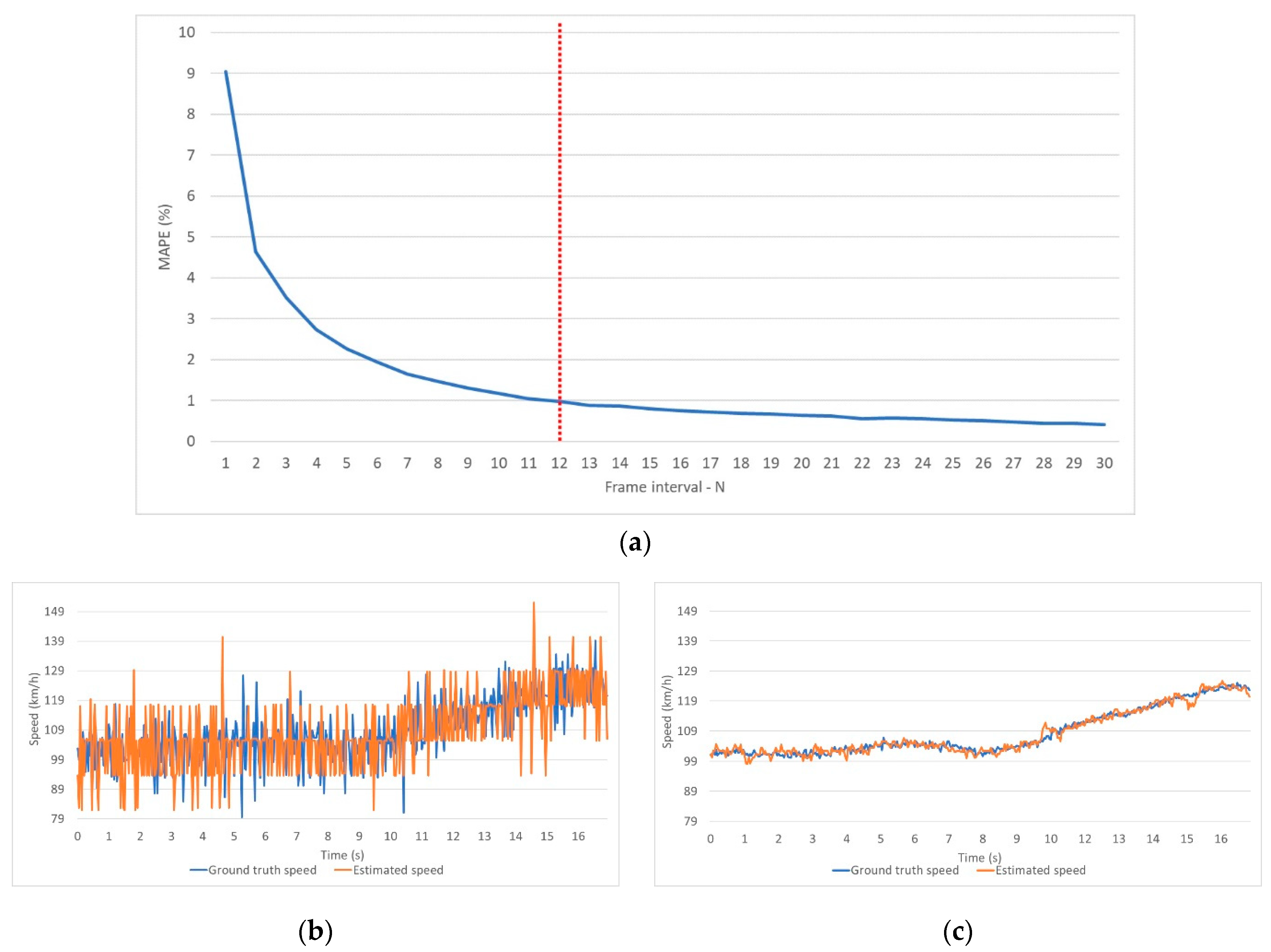
To determine which characteristic point of the bounding box will be used for tracking, RMSE was calculated for every characteristic point of the vehicle bounding box. Centroids proved to be the best choice with the lowest RMSE value (0.28 m). In addition to the characteristic point, frame interval (N) was determined to estimate the vehicle speed. Figure 9a shows the MAPE change for N in a range from 1 to 30 frames. According to Figure 9a, N was set to 12. Figure 9b shows a comparison of the ground truth speed of vehicle 139 and the estimated speed for the same vehicle with N = 1, while Figure 9c shows the same comparison but with N = 12.
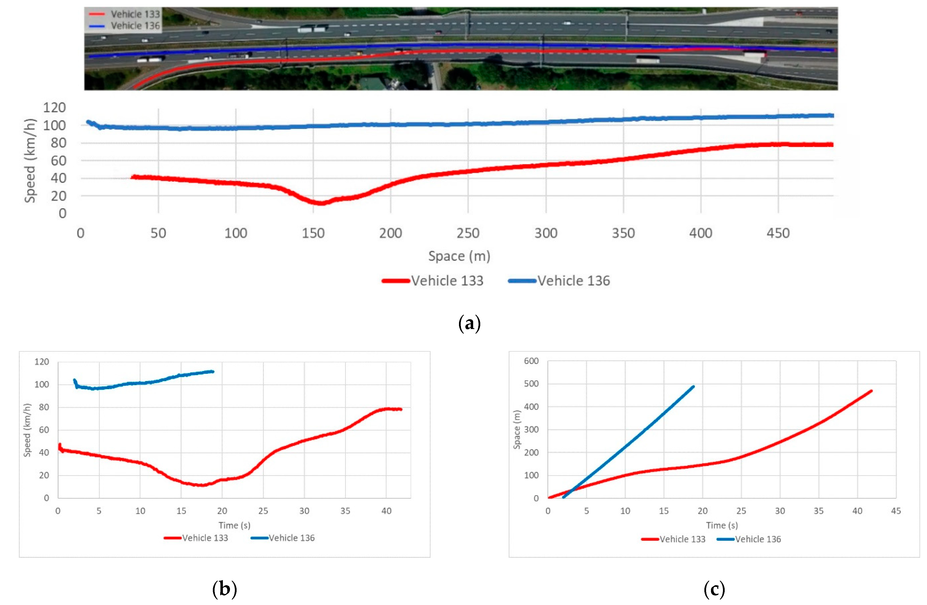
Subsequently, to demonstrate the possibilities of this framework, the trajectories of vehicles 133 and 136 are presented in this paper. For both selected vehicles, speed—space, speed—time and space—time diagrams were created (Figure 10). From Figure 10b, it is evident that vehicle 133 traveled approximately 480 m, while vehicle 139 traveled approximately 500 m. Moreover, it can be seen that vehicle 136 appears in the video approximately two seconds after vehicle 133. It can be seen from Figure 10c that vehicle 133 passed vehicle 136 at approximately the third second of the video.
Afterwards, the spatial resolution was calculated based on Equations (6)–8). The spatial distance between GCP1 and GCP2 is 486.24 m, while the image distance between the same points is 3740.31 pixels, resulting in a spatial resolution of 0.13 m. The calculated resolution was used to determine the traffic flow density as well as to determine the microscopic parameters. The calculated RMSEs for the characteristic points of the bounding boxes are shown in Table 4. Location-based parameters were calculated for all individual characteristic locations (Table 5). It is important to note that the upper left and upper right points of the bounding boxes were used to estimate the net time headway instead of the lower left and lower right points for better RMSE. The total IoU metric parameter is 0.876. Contrary to location-based parameters, the segment-based parameters were calculated for every single lane segment (Table 6).
4. Discussion
This framework provides a new approach to traffic flow parameter estimation. The proposed framework integrates UAV, high-precision GNSS technology, state-of-the-art object detection, and spatial operations to provide highly accurate microscopic traffic flow parameters. Particular emphasis was placed on achieving high accuracy. This is done with the Faster R-CNN object detection network, which is pre-trained on the COCO dataset. Although only 160 images were used for the fine-tuning process, the evaluation process resulted in a precision of 0.988 and a recall of 0.994. Although this paper does not propose a new detection method and does not use the same dataset as datasets in the related papers, there are given comparisons with object detection metrics of the related papers. The reason for that is based on the fact that success of the novel frameworks largely depends on the accuracy of object detection. In comparison with similar studies, Ke et al. achieved slightly better precision (0.995) and significantly lower recall (0.957) [14]. Considering that Ke et al. used 18,000 images for the training process, it consequently yields a very lengthy process. The exact duration time of the training process is not given by Ke et al. [14]. Since recall represents the ratio of detected and ground truth vehicles, in terms of vehicle detection it is more important to achieve a higher recall. False vehicles are usually detected at the same location of the observation area, so in the fluid traffic flow this can be eliminated by post-processing. In addition, false detected vehicles do not appear in the consecutive frames, so they cannot be tracked and therefore the estimation of the traffic flow parameters cannot be affected. Contrary to false detected vehicles, undetected vehicles cannot be detected in post-processing and can cause major errors in estimating the traffic flow parameters. For this reason, L. Wang et al., give only the number of detected and “lost” vehicles instead of the confusion matrix, while the precision value is not provided [17]. From the number of detected and “lost” vehicles it is clear that the recall of their vehicle detection is 0.979, which is less than the recall of vehicle detection used in this study. In addition to recall and precision, our study provides other evaluation metrics such as accuracy and F1 score that can be used in the future studies as benchmarks.
Since Faster R-CNN is a robust object detection network, it is advisable to analyze the ground truth objects and, according to the analysis, set the parameters for fine-tuning. In order to reduce the training time, it is important to specify the scales and aspect ratios of anchors with regards to the capacity of available hardware. For this reason, scales and aspect ratio are set to three values that are chosen to include all ground truth vehicles. Based on the distribution of vehicle sizes and aspect ratios, the scales were set to 3, 7, and 11, while the aspect ratios were set to 2, 4, and 6. Setting more values can even improve the evaluation metrics of vehicle detection, but this will yield an extension of the training time, with little benefit to precision.
To estimate the TMS and SMS, it is necessary to determine the frame interval. This type of analysis for the selection of appropriate frame interval for speed estimation has not yet been applied. For example, Ke et al., selected the frame interval of 5 in 25 Hz video, without a detailed explanation and mathematical analysis [14]. In this paper, the frame interval was selected based on the MAPE values of sample vehicle speed. As already established, a smaller interval will result in a higher MAPE rate, while larger intervals will result in a lower MAPE rate. The analysis of MAPE and frame intervals shows a decreasing MAPE rate while the frame interval is increasing. According to the MAPE—frame interval diagram, the frame interval is set to 12, which represents half of a second. Speed estimation, concerning the last half of a second, has a MAPE slightly below 1%, which represents a satisfactory rate. This study provides the difference between the speed values estimated for the frame interval from 1 to 12. The speed has higher amplitudes when the frame interval is 1, resulting in a higher MAPE rate. There are two reasons for high amplitudes. The first one is a spatial resolution for ground truth speed determination. The high spatial resolution allows the identification of characteristic details on the vehicle (rearview mirror, vehicle lights, etc.), and therefore allows the vehicle speed to be determined manually, with always tracking the same detail on the vehicle frame-by-frame. The described procedure for determining the speed of a ground truth will result in lower amplitudes of ground truth speed. Contrary to the high spatial resolution, the low resolution does not allow tracking vehicles by characteristic details. The characteristic detail points on the vehicle in each frame are determined by personal assessment. Another reason for the high amplitudes is the variable position of the vehicle centroid for each frame. The bounding boxes of one vehicle do not have the same relative position concerning the vehicle in each frame. This may cause large amplitudes of estimated speed when the frame interval is 1.
This framework provides the determination of trajectories for every single vehicle. This study provides trajectories of vehicles 133 and 136. These vehicles were selected to show the differences in speed and trajectory, given that vehicle 136 had a relatively light flow, while vehicle 133 slowed down when entering the highway. Our results provide the speed—space, speed—time, and space—time diagrams for the same vehicles. Considering all these diagrams can be drawn from the results of the proposed framework for vehicles 133 and 136, it is possible to analyze the relations between any vehicle in the video with frequency of 24 Hz. These relations are important for some other types of traffic analysis, such as determining the critical gap and shockwaves, or for energy and environmental analysis. For shockwave analysis, Khan et al. proposed a framework with optical flow, background subtraction and blob analysis for detecting and tracking vehicles from a UAV-based video [13]. They do not provide any metrics on detection accuracy, so from this point of view these frameworks cannot be compared. However, they did provide a MAPE rate for one vehicle of 5.85%. Given that the MAPE rate of speed estimation for our framework is 0.92%, it is a significant difference. The reason for the lower MAPE rate may be that we analyzed the decrease in MAPE rate with increasing the frame interval, and according to the already described analysis, we selected 12 frames as the optimal frame interval. They also recorded a traffic flow with the UAV placed eccentrically concerning the observed area, while we placed the UAV approximately perpendicular to the observed area. Fedorov et al., used a surveillance camera for recording the road intersection and highlight the problem of overlapping vehicles caused by oblique recording [16]. Therefore, placing the UAV approximately perpendicular to the observed area has great influence on determining the spatial relations between vehicles, especially in the analysis of critical gaps and shockwaves.
Moreover, this framework enables the estimation of microscopic traffic flow parameters. Except for Khan et al., other related papers do not provide microscopic parameters [13]. The reason for this may be a highly accurate determination of the spatial resolution, which is significant for the measurement and estimation of microscopic parameters. Our proposed framework includes GNSS technology for determining a highly accurate spatial resolution. Since UAVs usually have a single-frequency GNSS, it is more accurate to use a dual-frequency GNSS receiver to determine the spatial resolution instead of spatial resolution calculation from the sensor dimensions, focal length, and UAV flight altitude.
Finally, the implementation of the proposed framework allows the determination of traffic flow parameters for each individual lane. The boundary boxes of detected vehicles and motorway lanes can be considered as spatial objects, i.e. polygons. This allows spatial analysis to be applied to them. The use of spatial analysis enables the automatic estimation of microscopic parameters of the traffic flow. A review of the related literature shows that this approach to determining microscopic parameters has not yet been applied [13,14,16,17].
In addition to all these advantages, the proposed framework has several limitations. First, the flight time of the UAV is limited, which does not allow the observation of the area of interest for more than a short period of time, depending on the capacity of the battery. Short flight times can be a significant problem in estimating reliable traffic flow parameters. This problem can be partially solved by observing the road over several periods of time during the day and it is highly dependent on the traffic volume at the given locations. Shorter observations provide a sufficient number of detections at high volumes while on low-volume sections multiple flights are required. This can be performed if multiple batteries are available, but the complete solution will only be achieved with an increase in the UAV battery capacity. Second, the framework is not fully automated. The vehicle detection segment of the framework requires manual labeling of the vehicle to fine-tune the Faster R-CNN networks. Although a small set of images is required for the fine-tuning process, it is short-lived and it prevents frame automation. Third, UAVs represent a significantly more affordable solution for determining the flow parameters than the currently used technologies such as inductive loops, pneumatic road pipes, etc.
5. Conclusions
This paper provides a new framework for determining the traffic flow parameters. The proposed framework represents a more affordable and more efficient approach for typical standard traffic flow parameters determination than the techniques that are in current use. Furthermore, this method provides a simple and accurate method for plotting vehicle trajectories and continuous headway measurements at road sections that are not available with traditional traffic flow survey methods. The proposed framework can be segmented into a terrain survey, image processing, vehicle detection, and parameter estimation. Particular emphasis is placed on achieving high accuracy. To achieve high accuracy, Faster R-CNN network was used. It is a robust state-of-the-art network, which was pre-trained with COCO image dataset and fine-tuned with only 160 training images. Using a fine-tuned Faster R-CNN network for vehicle detection achieved a recall of 0.994, which is significantly higher than the detection recalls in the related papers. Moreover, the proposed framework provides a vehicle speed estimation with a MAPE of 0.92%, which is satisfactory and allows the estimation of the trajectories for each individual vehicle in the video.
Future studies will focus on addressing these shortcomings and improving the proposed framework. Particular emphasis should be placed on creating large datasets containing labeled vehicles in images from different videos and different contexts.
Author Contributions
Conceptualization, I.B. and M.M.; investigation, I.B.; methodology, I.B., M.Š., and M.M.; supervision, M.M., M.Š., and D.M.; validation, I.B. and M.M.; visualization, I.B.; writing—original draft, I.B.; writing—review and editing, M.M., M.Š., and D.M.; funding acquisition, D.M. All authors have read and agreed to the published version of the manuscript.
Funding
This work was supported by the Croatian Science Foundation for the GEMINI project: “Geospatial Monitoring of Green Infrastructure by Means of Terrestrial, Airborne, and Satellite Imagery” (Grant No. HRZZ-IP-2016-06-5621).
Conflicts of Interest
The authors declare no conflict of interest.
References
- European Automobile Manufacturers Association Vehicles in use Europe 2019. 2019. Available online: https://www.acea.be/uploads/statistic_documents/ACEA_Report_Vehicles_in_use-Europe_2017.pdf (accessed on 10 March 2020).
- Mathew, T.V.; Rao, K.V.K. Fundamental parameters of traffic flow. In Introduction to Transportation Engineering; National Program on Technical Education and Learning (NPTEL): Mumbay, India, 2007; pp. 1–8. [Google Scholar]
- Hoogendoorn, S.; Knoop, V. Traffic flow theory and modelling. Transp. Syst. Transp. Policy Introd. 2012, 125–159. [Google Scholar]
- Leduc, G. Road Traffic Data: Collection Methods and Applications; JRC: Seville, Spain, 2008. [Google Scholar]
- Handscombe, J.; Yu, H.Q. Low-Cost and Data Anonymised City Traffic Flow Data Collection to Support Intelligent Traffic System. Sensors 2019, 19, 347. [Google Scholar] [CrossRef] [PubMed] [Green Version]
- Martinez, A.P. Freight Traffic data in the City of Eindhoven; University of Technology Eindhoven: Eindhoven, The Netherlands, 2015. [Google Scholar]
- Kanistras, K.; Martins, G.; Rutherford, M.J.; Valavanis, K.P. A survey of unmanned aerial vehicles (UAVs) for traffic monitoring. In Proceedings of the 2013 International Conference on Unmanned Aircraft Systems (ICUAS), Atlanta, GA, USA, 28–31 May 2013; pp. 221–234. [Google Scholar]
- SESAR Joint Undertaking European Drones Outlook Study. SESAR 2016. Available online: http://www.sesarju.eu/sites/default/files/documents/reports/European_Drones_Outlook_Study_2016.pdf (accessed on 12 March 2020).
- El-Sayed, H.; Chaqfa, M.; Zeadally, S.; Puthal, A.D. A Traffic-Aware Approach for Enabling Unmanned Aerial Vehicles ( UAVs ) in Smart City Scenarios. IEEE Access 2019, 7, 86297–86305. [Google Scholar] [CrossRef]
- Menouar, H.; Guvenc, I.; Akkaya, K.; Uluagac, A.S.; Kadri, A.; Tuncer, A. UAV-Enabled Intelligent Transportation Systems for the Smart City: Applications and Challenges. IEEE Commun. Mag. 2017, 55, 22–28. [Google Scholar] [CrossRef]
- Ghazzai, H.; Menouar, H.; Kadri, A. On the Placement of UAV Docking Stations for Future Intelligent Transportation Systems. In Proceedings of the 2017 IEEE 85th Vehicular Technology Conference (VTC Spring), Sydney, Australia, 4–7 June 2017; pp. 1–6. [Google Scholar]
- Beg, A.; Qureshi, A.R.; Sheltami, T.; Yasar, A. UAV-enabled intelligent traffic policing and emergency response handling system for the smart city. Pers. Ubiquitous Comput. 2020, 1–18. [Google Scholar] [CrossRef]
- Khan, M.A.; Ectors, W.; Bellemans, T.; Janssens, D.; Wets, G. Unmanned Aerial Vehicle-Based Traffic Analysis: A Case Study for Shockwave Identification and Flow Parameters Estimation at Signalized Intersections. Remote Sens. 2018, 10, 458. [Google Scholar] [CrossRef] [Green Version]
- Ke, R.; Li, Z.; Tang, J.; Pan, Z.; Wang, Y. Real-Time Traffic Flow Parameter Estimation From UAV Video Based on Ensemble Classifier and Optical Flow. IEEE Trans. Intell. Transp. Syst. 2019, 20, 54–64. [Google Scholar] [CrossRef]
- Chen, X.; Li, Z.; Yang, Y.; Qi, L.; Ke, R. High-Resolution Vehicle Trajectory Extraction and Denoising From Aerial Videos. IEEE Trans. Intell. Transp. Syst. 2020, 1–13. [Google Scholar] [CrossRef]
- Fedorov, A.; Nikolskaia, K.; Ivanov, S.; Shepelev, V.; Minbaleev, A. Traffic flow estimation with data from a video surveillance camera. J. Big Data 2019, 6. [Google Scholar] [CrossRef]
- Wang, L.; Chen, F.; Yin, H. Detecting and tracking vehicles in traffic by unmanned aerial vehicles. Autom. Constr. 2016, 72, 294–308. [Google Scholar] [CrossRef]
- Transport Development Strategy of the Republic of Croatia (2017–2030)—Development of Sectoral Transport Strategies; Ministry of the Sea, Transport and Infrastructure: Zagreb, Croatia, 2013; ISBN 9788578110796.
- Transportation Research Board. Highway Capacity Manual 6th Edition: A Guide for Multimodal Mobility Analysis; The National Academies Press: Washington, DC, USA, 2016. [Google Scholar] [CrossRef]
- Awad, A.I.; Hassaballah, M. (Eds.) Studies in Computational Intelligence; Springer International Publishing: Cham, Switzerland, 2016; Volume 630, ISBN 978-3-319-28852-9. [Google Scholar]
- Pieropan, A.; Björkman, M.; Bergström, N.; Kragic, D. Feature Descriptors for Tracking by Detection: A Benchmark. arXiv 2016, arXiv:1607.06178. [Google Scholar]
- Aglave, P.; Kolkure, V.S. Implementation of High Performance Feature Extraction Method Using Oriented Fast and Rotated Brief Algorithm. Int. J. Res. Eng. Technol. 2015, 4, 394–397. [Google Scholar] [CrossRef]
- Zhou, Q.; Li, X. STN-Homography: Estimate homography parameters directly. arXiv 2019, arXiv:1906.02539. [Google Scholar]
- Chum, O.; Matas, J.; Kittler, J. Locally optimized RANSAC. In Proceedings of the Joint Pattern Recognition Symposium; Springer: Berlin/Heidelberg, Germany, 2003; Volume 2781, pp. 236–243. [Google Scholar]
- Fischler, M.A.; Bolles, R.C. Random Sample Consensus: A Paradigm for Model Fitting with Applications to Image Analysis and Automated Cartography; Morgan Kaufmann Publishers, Inc.: Burlington, MA, USA, 1987. [Google Scholar]
- Ma, Y.; Soatto, S.; Košecká, J.; Sastry, S.S. Reconstruction from Two Uncalibrated Views. In An Invitation to 3-D Vision; Springer: Berlin/Heidelberg, Germany, 2004; pp. 171–227. [Google Scholar]
- Yague-Martinez, N.; De Zan, F.; Prats-Iraola, P. Coregistration of Interferometric Stacks of Sentinel-1 TOPS Data. IEEE Geosci. Remote Sens. Lett. 2017, 14, 1002–1006. [Google Scholar] [CrossRef] [Green Version]
- Zhao, Z.-Q.; Zheng, P.; Xu, S.-T.; Wu, X. Object Detection With Deep Learning: A Review. IEEE Trans. Neural Netw.Learn. Syst. 2019, 30, 3212–3232. [Google Scholar] [CrossRef] [PubMed] [Green Version]
- JJiao, L.; Zhang, F.; Liu, F.; Yang, S.; Li, L.; Feng, Z.; Qu, R. A Survey of Deep Learning-Based Object Detection. IEEE Access 2019, 7, 128837–128868. [Google Scholar] [CrossRef]
- Li, B.; Liu, Y.; Wang, X. Gradient Harmonized Single-Stage Detector. Proc Conf AAAI Artif Intell 2019, 33, 8577–8584. [Google Scholar] [CrossRef]
- Sun, B.; Xu, Y.; Li, C.; Yu, J. Analysis of the Impact of Google Maps’ Level on Object Detection. In Proceedings of the IGARSS 2019—2019 IEEE International Geoscience and Remote Sensing Symposium, Yokohama, Japan, 28 July–2 August 2019; pp. 1248–1251. [Google Scholar]
- Liu, L.; Ouyang, W.; Wang, X.; Fieguth, P.; Chen, J.; Liu, X.; Pietikäinen, M. Deep Learning for Generic Object Detection: A Survey. Int. J. Comput. Vis. 2020, 128, 261–318. [Google Scholar] [CrossRef] [Green Version]
- Lin, T.Y.; Maire, M.; Belongie, S.; Hays, J.; Perona, P.; Ramanan, D.; Dollár, P.; Zitnick, C.L. Microsoft COCO: Common objects in context. In Proceedings of the European Conference on Computer Vision; Springer: Berlin/Heidelberg, Germany, 2014; pp. 740–755. [Google Scholar]
- Ren, S.; He, K.; Girshick, R.; Sun, J. Faster R-CNN: Towards Real-Time Object Detection with Region Proposal Networks. IEEE Trans. Pattern Anal. Mach. Intell. 2017, 39, 1137–1149. [Google Scholar] [CrossRef] [Green Version]
- Wang, J.; Chen, K.; Yang, S.; Loy, C.C.; Lin, D. Region Proposal by Guided Anchoring. In Proceedings of the IEEE Conference on Computer Vision and Pattern Recognition, Long Beach, CA, USA, 16–21 June 2019. [Google Scholar]
- He, K.; Zhang, X.; Ren, S.; Sun, J. Deep residual learning for image recognition. In Proceedings of the IEEE Conference on Computer Vision and Pattern Recognition, Las Vegas, NV, USA, 27–30 June 2016; pp. 770–778. [Google Scholar]
- Mohammad, H.; Md Nasair, S. A Review on Evaluation Metrics for Data Classification Evaluations. Int. J. Data Min. Knowl. Manag. Process 2015, 5, 1–11. [Google Scholar]
- Authority, T.V. Federal Geographical Data Committee Geospatial Positioning Accuracy Standards Part 3: National Standard for Spatial Data Accuracy; National Aeronautics and Space Administration: Virginia, NV, USA, 1998; p. 10. [Google Scholar]
- Bewley, A.; Ge, Z.; Ott, L.; Ramos, F.; Upcroft, B. Simple online and realtime tracking. In Proceedings of the 2016 IEEE International Conference on Image Processing (ICIP), Phoenix, AZ, USA, 25–28 September 2016; pp. 3464–3468. [Google Scholar]
- Jordahl, K. GeoPandas Documentation 2016. Available online: https://buildmedia.readthedocs.org/media/pdf/geopandas/master/geopandas.pdf (accessed on 20 March 2020).
- Guo, J.; Huang, W.; Williams, B.M. Adaptive Kalman filter approach for stochastic short-term traffic flow rate prediction and uncertainty quantification. Transp. Res. Part C Emerg. Technol. 2014, 43, 50–64. [Google Scholar] [CrossRef]
- Mathew, T.V.; Rao, K.V.K. Fundamental relations of traffic flow. Introd. Transp. Eng. 2006, 1, 1–8. [Google Scholar]
- Turner, S.M.; Eisele, W.L.; Benz, R.J.; Douglas, J. Travel time data collection handbook. Fed. Highw. Adm. USA 1998, 3, 293. [Google Scholar]
- Knoop, V.; Hoogendoorn, S.P.; Van Zuylen, H. Empirical Differences Between Time Mean Speed and Space Mean Speed. Traffic Granul. Flow 07 2009, 351–356. [Google Scholar] [CrossRef]
- Dadić, I.; Kos, G.; Ševrović, M. Traffic Flow Theory. 2014. Available online: http://files.fpz.hr/Djelatnici/msevrovic/Teorija-prometnih-tokova-2014-skripta.pdf (accessed on 22 March 2020).
- Luttinen, R.T. Statistical Analysis of Vehicle Time Headways; University of Technology Lahti Center: Lahti, Finland, 1996. [Google Scholar]
Figure 1.
Location of the observed area on the Open Street Map and Croatian digital orthophoto from 2018 along with the image recorded from Unmanned Aerial Vehicles (UAV) whence Ground Control Points (GCPs) were marked.
Figure 1.
Location of the observed area on the Open Street Map and Croatian digital orthophoto from 2018 along with the image recorded from Unmanned Aerial Vehicles (UAV) whence Ground Control Points (GCPs) were marked.

Figure 2.
Proposed framework for the determination of traffic flow parameters.

Figure 3.
Image processing segment: firstly, frames were extracted from the video, then image alignment was applied, and finally, a narrow motorway area was cropped.
Figure 3.
Image processing segment: firstly, frames were extracted from the video, then image alignment was applied, and finally, a narrow motorway area was cropped.

Figure 4.
(a) Characteristic points of bounding boxes; (b) example of difference between ground truth and estimated bounding boxes.
Figure 4.
(a) Characteristic points of bounding boxes; (b) example of difference between ground truth and estimated bounding boxes.

Figure 5.
Marked characteristic locations of the observed area used for calculating location-based traffic flow parameters.
Figure 5.
Marked characteristic locations of the observed area used for calculating location-based traffic flow parameters.

Figure 6.
Marked lane segments of the observed area used for calculating segment-based traffic flow parameters.
Figure 6.
Marked lane segments of the observed area used for calculating segment-based traffic flow parameters.

Figure 7.
The difference between headways and gaps; red line marks the reference line for measuring location-based microscopic parameters such as time headways and gaps.
Figure 7.
The difference between headways and gaps; red line marks the reference line for measuring location-based microscopic parameters such as time headways and gaps.

Figure 8.
(a) Distribution of vehicles in the training set based on their scales and aspect ratios if anchor size is set to 16 × 16 pixels; (b) distribution of vehicle sizes based on height and width of their bounding boxes.
Figure 8.
(a) Distribution of vehicles in the training set based on their scales and aspect ratios if anchor size is set to 16 × 16 pixels; (b) distribution of vehicle sizes based on height and width of their bounding boxes.

Figure 9.
(a) MAPE—Frame interval diagram showing a decrease in MAPE as the number of frame intervals increases, the selected optimal frame interval is determined by the red line. (b) Time—speed diagram for ground truth and estimated data of vehicle 139 with N = 1; it is visible that speeds of estimated and ground truth bounding boxes have high rate of noise. (c) Time—speed diagram for ground truth and estimated data of vehicle 139 with N = 12; it is visible that the increase in frame interval causes a smoother speed curve.

Figure 10.
(a) Trajectories of vehicles 133 and 136 and their change of speed during travel. (b) Speed—time diagram of vehicles 133 and 136. (c) Space—time diagram of vehicles 133 and 136.
Figure 10.
(a) Trajectories of vehicles 133 and 136 and their change of speed during travel. (b) Speed—time diagram of vehicles 133 and 136. (c) Space—time diagram of vehicles 133 and 136.


Table 1.
Table of parameters and their values used in Faster R-CNN ResNet50 COCO network.
| Name of Parameters | Value |
|---|---|
| Height of anchors | 16 |
| Width of anchors | 16 |
| Height stride | 16 |
| Width stride | 16 |
| Aspect ratios | 2, 4, 6 |
| Scales | 3, 7, 11 |
Table 2.
Confusion matrix of test dataset.
| Actual | |||
|---|---|---|---|
| Vehicle | Not vehicle | ||
| Predicted | Vehicle | 1070 | 13 |
| Not vehicle | 6 | 0 | |
Table 3.
Evaluating metrics of test dataset.
| Evaluate Metric | Value |
|---|---|
| Precision | 0.988 |
| Recall | 0.994 |
| Accuracy | 0.983 |
| F1 score | 0.991 |
Table 4.
Root Mean Square Error (RMSE) value of characteristic points.
| Characteristic Point | RMSE Value (m) |
|---|---|
| Upper left | 0.432 |
| Upper right | 0.360 |
| Bottom left | 0.405 |
| Bottom right | 0.397 |
Table 5.
Estimated location-based traffic flow parameters.
| Location ID | Traffic Flow Rate | TMS (km/h) | Time Headways and Gaps | ||
|---|---|---|---|---|---|
| Counted Number of Vehicles | Estimated Number of Vehicles (vehicles/h) | Time Headway (s) | Time Gap (s) | ||
| 1 | 96 | 411 | 75.03 | 8.61 | 8.06 |
| 2a | 194 | 831 | 75.76 | 4.37 | 3.7 |
| 2b | 300 | 1286 | 98.14 | 2.87 | 2.5 |
| 3a | 191 | 819 | 80.64 | 4.26 | 3.75 |
| 3b | 243 | 1041 | 106.36 | 3.33 | 3.11 |
| 4 | 92 | 394 | 74.48 | 8.34 | 8.03 |
| 5 | 91 | 390 | 51.44 | 8.52 | 7.95 |
| 6a | 206 | 883 | 81.91 | 3.97 | 3.51 |
| 6b | 293 | 1256 | 101.67 | 2.79 | 2.58 |
| 7a | 184 | 789 | 79.22 | 4.65 | 3.92 |
| 7b | 247 | 1059 | 104.63 | 3.38 | 3.07 |
| 8 | 95 | 407 | 80.85 | 8.83 | 8.33 |
Table 6.
Estimated segment-based traffic flow parameters.
| Lane Segment ID | Average SMS (km/h) | Average Density (vehicles/km) | Distance Headways and Gaps | |
|---|---|---|---|---|
| Distance Headway (m) | Distance Gap (m) | |||
| 1 | 64.88 | 5 | 70.33 | 64.29 |
| 2 | 77.76 | 10 | 76.06 | 66.69 |
| 3 | 98.89 | 13 | 56.77 | 51.17 |
| 4 | 104.70 | 10 | 70.98 | 65.32 |
| 5 | 81.83 | 10 | 82.51 | 72.44 |
| 6 | 70.08 | 5 | 73.40 | 67.14 |
Publisher’s Note: MDPI stays neutral with regard to jurisdictional claims in published maps and institutional affiliations. |
© 2020 by the authors. Licensee MDPI, Basel, Switzerland. This article is an open access article distributed under the terms and conditions of the Creative Commons Attribution (CC BY) license (http://creativecommons.org/licenses/by/4.0/).
Share and Cite
MDPI and ACS Style
Brkić, I.; Miler, M.; Ševrović, M.; Medak, D. An Analytical Framework for Accurate Traffic Flow Parameter Calculation from UAV Aerial Videos. Remote Sens. 2020, 12, 3844. https://0-doi-org.brum.beds.ac.uk/10.3390/rs12223844
AMA Style
Brkić I, Miler M, Ševrović M, Medak D. An Analytical Framework for Accurate Traffic Flow Parameter Calculation from UAV Aerial Videos. Remote Sensing. 2020; 12(22):3844. https://0-doi-org.brum.beds.ac.uk/10.3390/rs12223844
Chicago/Turabian StyleBrkić, Ivan, Mario Miler, Marko Ševrović, and Damir Medak. 2020. "An Analytical Framework for Accurate Traffic Flow Parameter Calculation from UAV Aerial Videos" Remote Sensing 12, no. 22: 3844. https://0-doi-org.brum.beds.ac.uk/10.3390/rs12223844
Note that from the first issue of 2016, this journal uses article numbers instead of page numbers. See further details here.