Combining Evolutionary Algorithms and Machine Learning Models in Landslide Susceptibility Assessments


Abstract
:
1. Introduction
2. Study Area
3. Materials and Methods
3.1. Methodology
3.1.1. First Phase
3.1.2. Second Phase
3.1.3. Third Phase
3.1.4. Fourth Phase
3.1.5. Fifth Phase
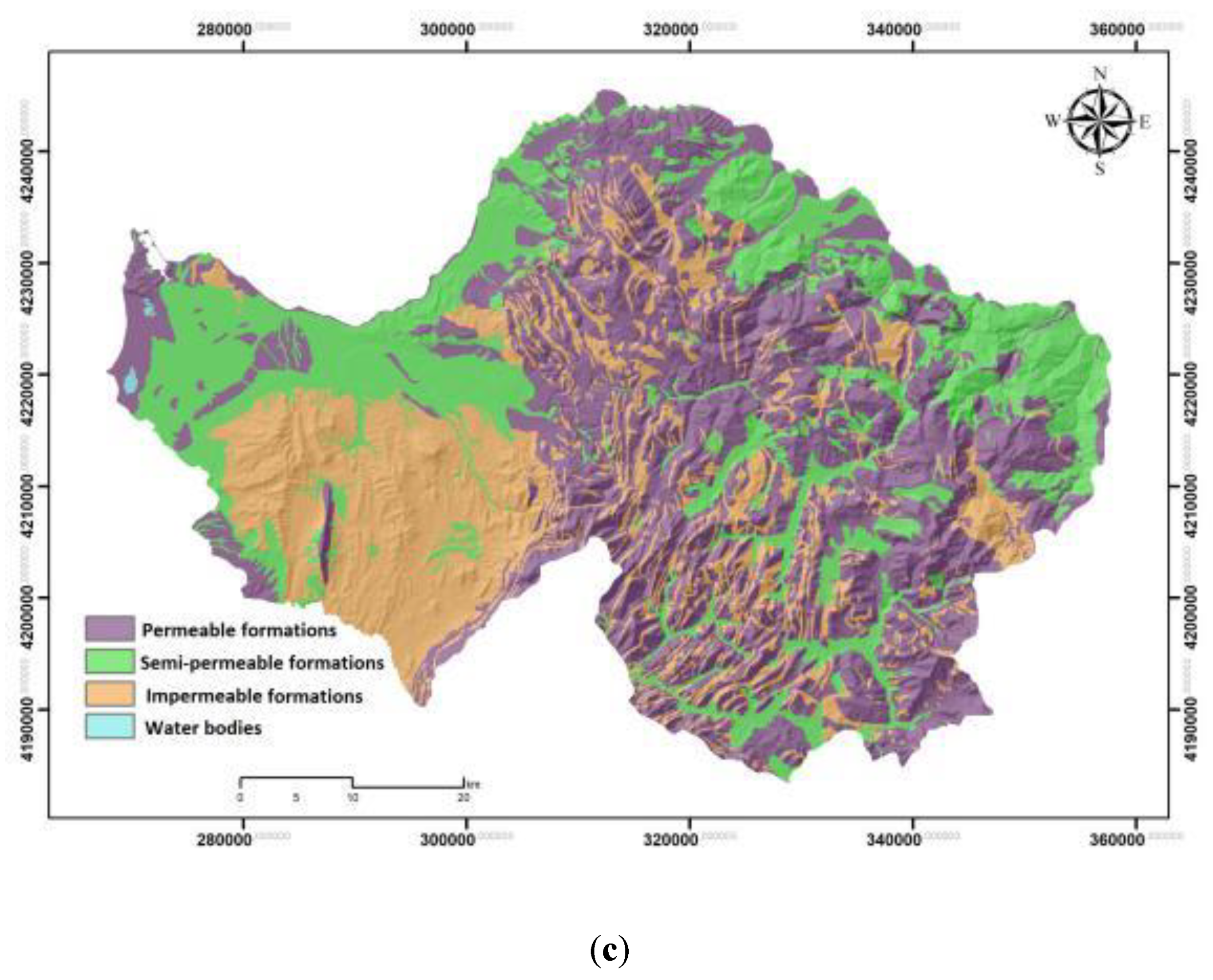
3.2. Data
4. Results
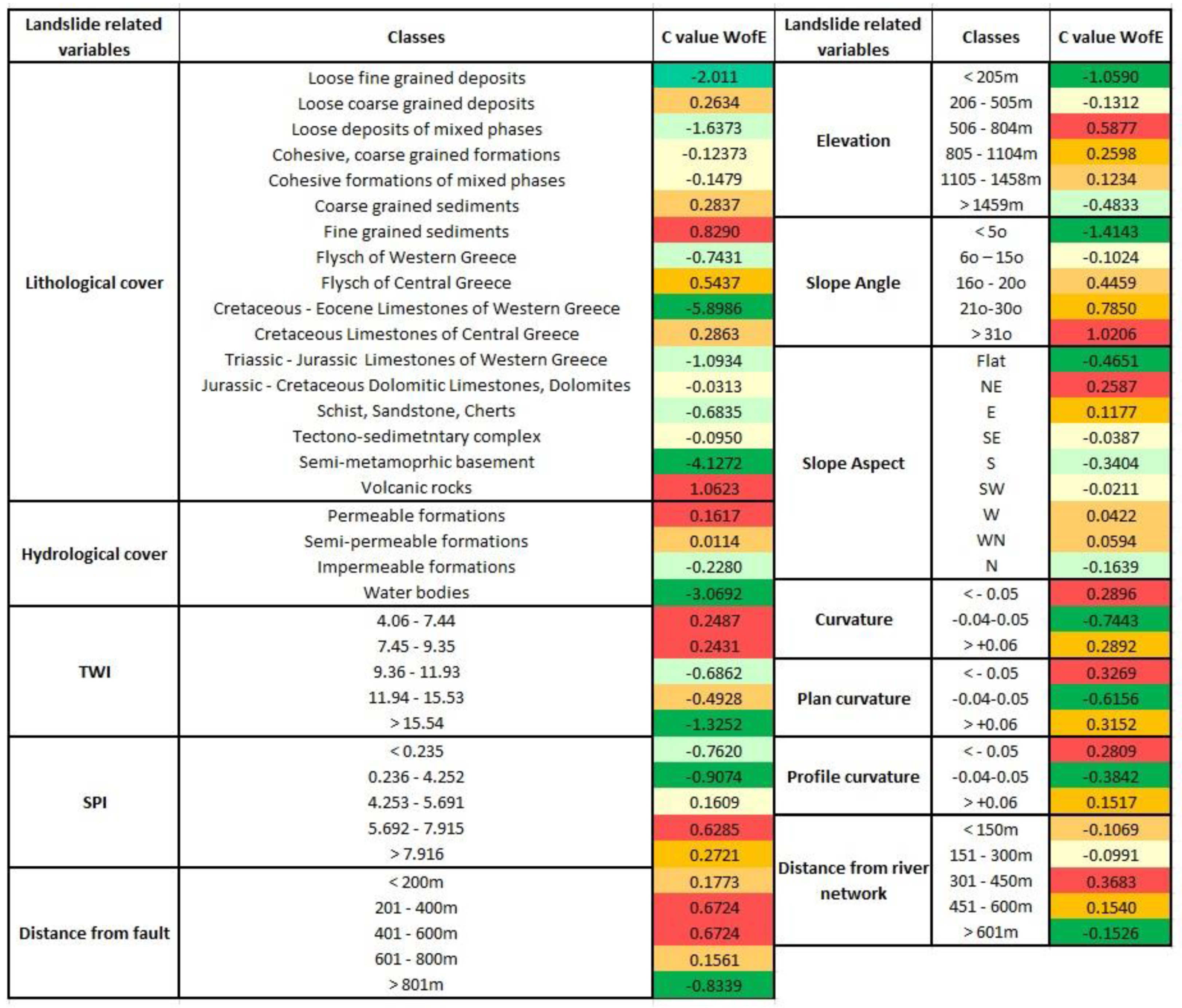
4.1. First Phase—WofE Analysis
4.2. Second Phase—Multi-Collinearity Analysis
4.3. Third Phase—Feature Selection by GA
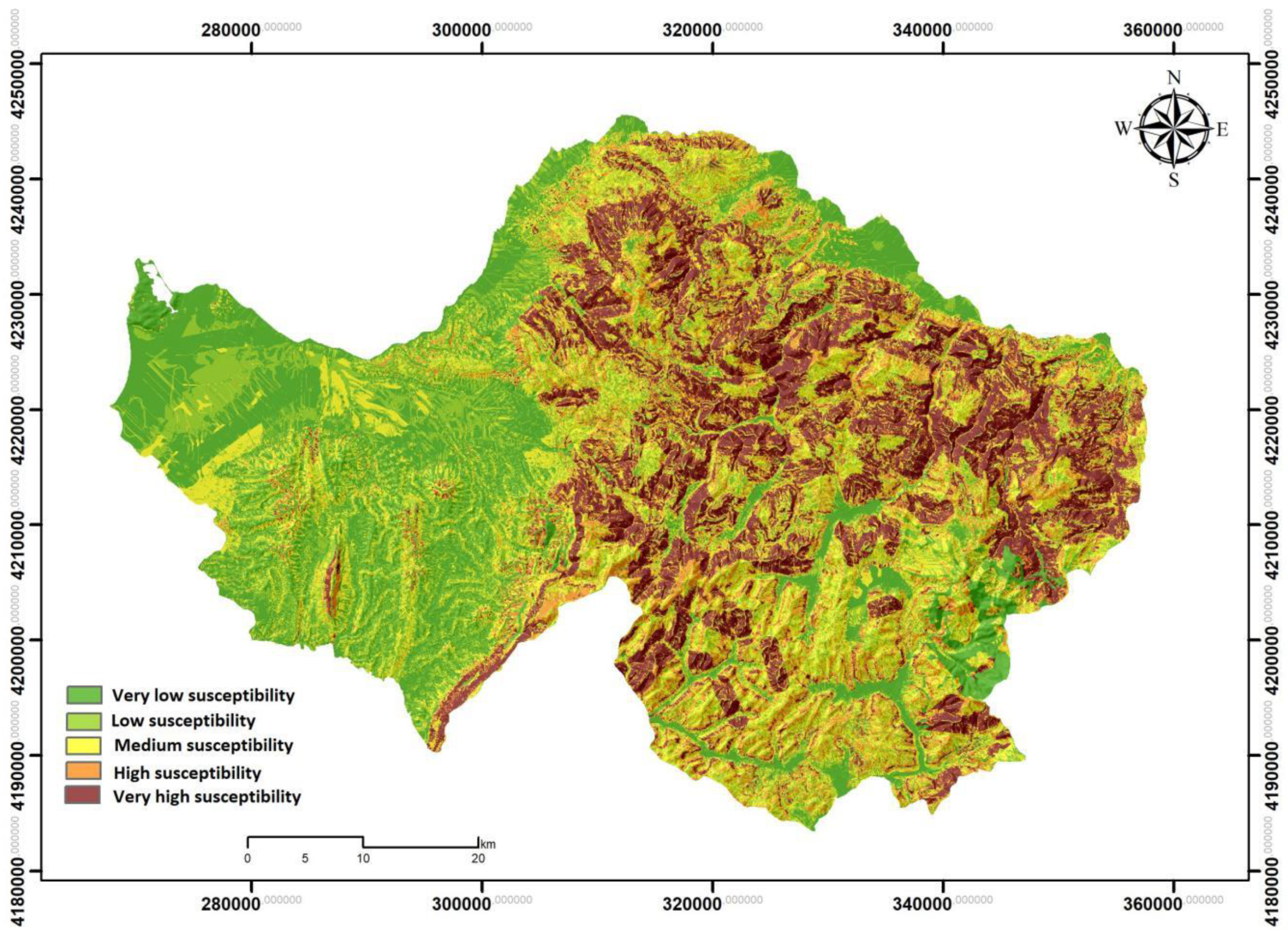
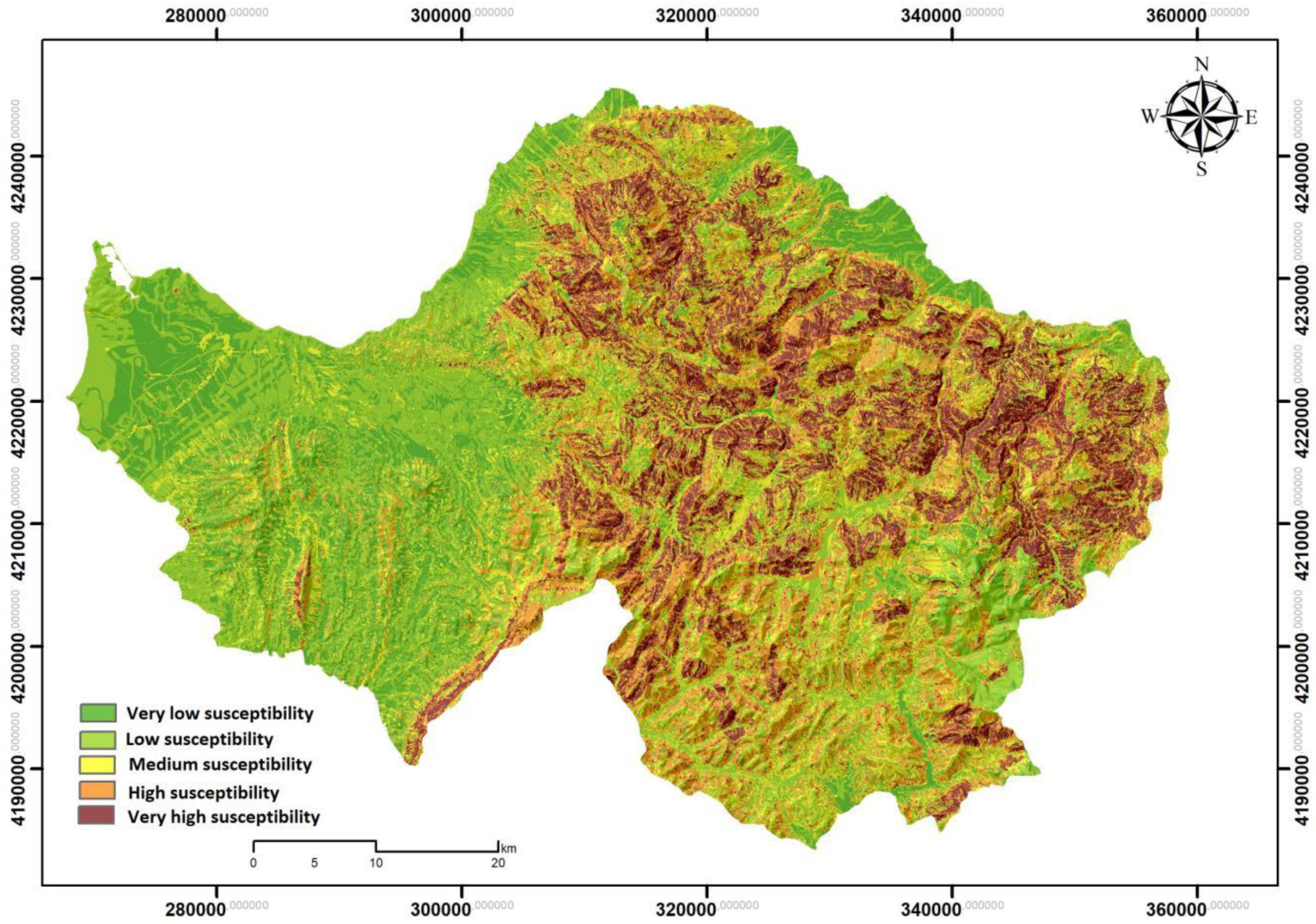
4.4. Fourth Phase—Optimizing SVM and ANN by PSO for Landslide Susceptibility Mapping
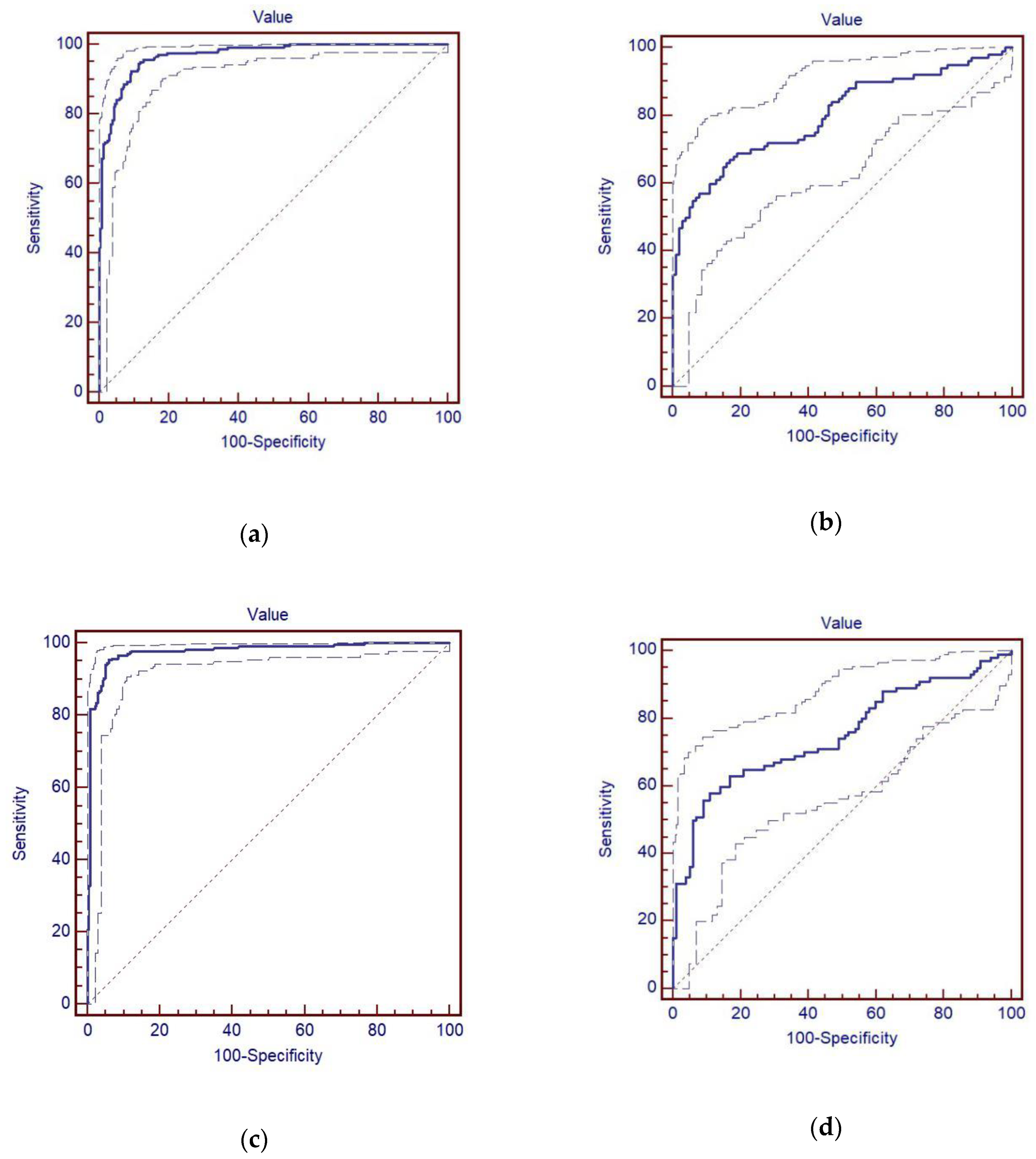
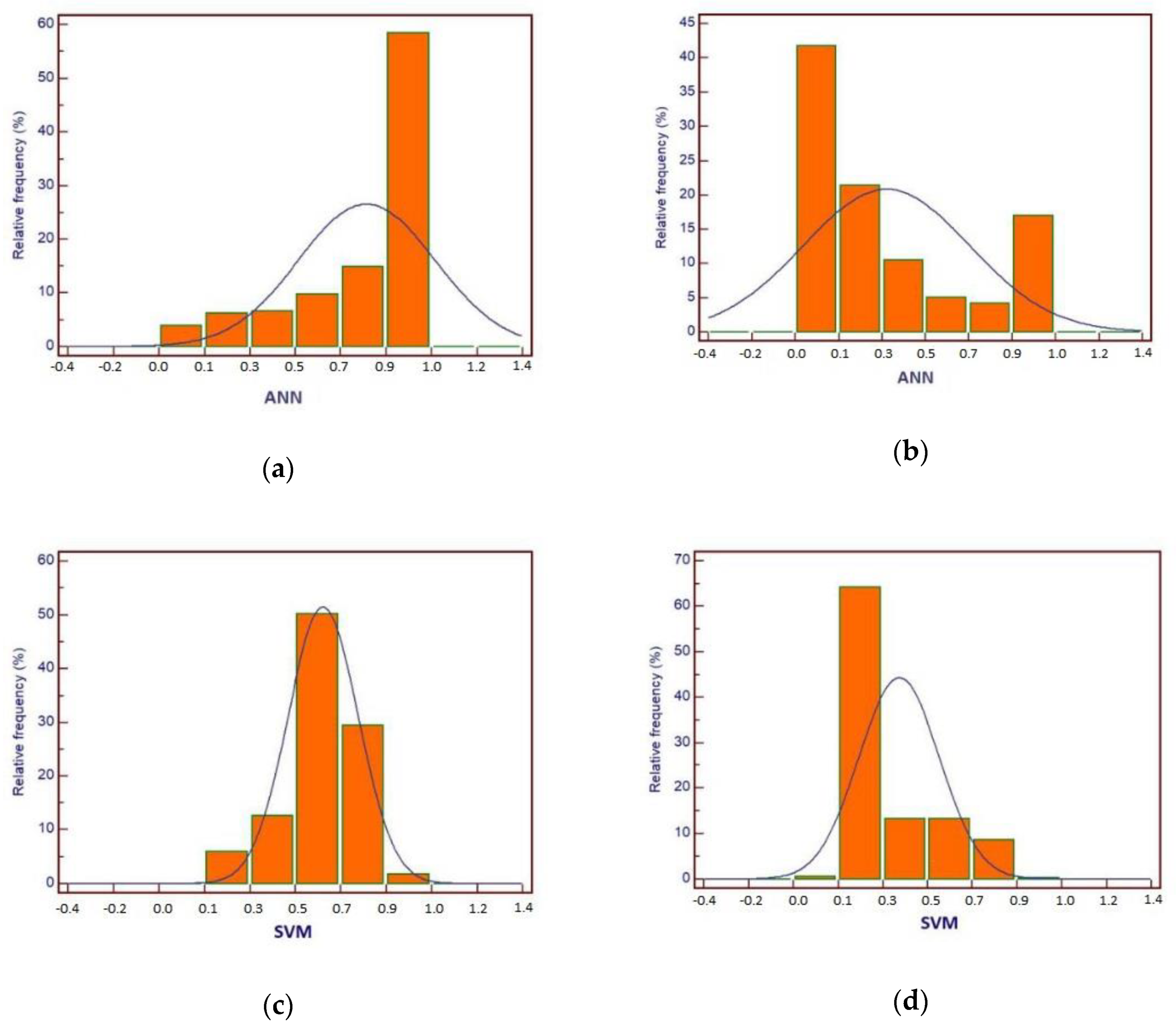
4.5. Fifth Phase—Evaluating the Performance of the SVM and ANN
5. Discussion
6. Conclusions
Author Contributions
Funding
Acknowledgments
Conflicts of Interest
References
- Feizizadeh, B.; Blaschke, T. An uncertainty and sensitivity analysis approach for GIS-based multicriteria landslide susceptibility mapping. Int. J. Geogr. Inf. Sci. 2014, 28, 610–638. [Google Scholar] [CrossRef] [PubMed] [Green Version]
- Reichenbach, P.; Rossi, M.; Malamud, B.D.; Mihir, M.; Guzzetti, F. A review of statistically-based landslide susceptibility models. Earth Sci. Rev. 2018, 180, 60–91. [Google Scholar] [CrossRef]
- Kirschbaum, D.; Stanley, T.; Zhou, Y. Spatial and temporal analysis of a global landslide catalog. Geomorphology 2015, 249, 4–15. [Google Scholar] [CrossRef]
- Zare, M.; Pourghasemi, H.R.; Vafakhah, M.; Pradhan, B. Landslide susceptibility mapping at Vaz Watershed (Iran) using an artificial neural network model: A comparison between multilayer perceptron (MLP) and radial basic function (RBF) algorithms. Arab. J. Geosci. 2013, 6, 2873–2888. [Google Scholar] [CrossRef]
- Hong, H.; Tsangaratos, P.; Ilia, I.; Loupasakis, C.; Wang, Y. Introducing a novel multi-layer perceptron network based on stochastic gradient descent optimized by a meta-heuristic algorithm for landslide susceptibility mapping. Sci. Total Environ. 2020, 742, 140549. [Google Scholar] [CrossRef]
- Korup, O.; Stolle, A. Landslide prediction from machine learning. Geol. Today 2014, 30, 26–33. [Google Scholar] [CrossRef]
- Pham, B.T.; Bui, D.T.; Prakash, I. Bagging based Support Vector Machines for spatial prediction of landslides. Environ. Earth Sci. 2018, 77, 146. [Google Scholar] [CrossRef]
- Ayalew, L.; Yamagishi, H. The application of GIS-based logistic regression for landslide susceptibility mapping in the Kakuda-Yahiko Mountains, Central Japan. Geomorphology 2005, 65, 15–31. [Google Scholar] [CrossRef]
- Pradhan, B.; Lee, S. Landslide susceptibility assessment and factor effect analysis: Backpropagation artificial neural networks and their comparison with frequency ratio and bivariate logistic regression modelling. Environ. Model. Softw. 2010, 25, 747–759. [Google Scholar] [CrossRef]
- Pradhan, B. Landslide susceptibility mapping of a catchment area using frequency ratio, fuzzy logic and multivariate logistic regression approaches. J. Indian Soc. Remote Sens. 2010, 38, 301–320. [Google Scholar] [CrossRef]
- Pham, B.T.; Pradhan, B.; Bui, D.T.; Prakash, I.; Dholakia, M. A comparative study of different machine learning methods for landslide susceptibility assessment: A case study of Uttarakhand area (India). Environ. Model. Softw. 2016, 84, 240–250. [Google Scholar] [CrossRef]
- Zhou, C.; Yin, K.; Cao, Y.; Ahmed, B.; Li, Y.; Catani, F.; Pourghasemi, H.R. Landslide susceptibility modeling applying machine learning methods: A case study from Longju in the Three Gorges Reservoir area, China. Comput. Geosci. 2018, 112, 23–37. [Google Scholar] [CrossRef] [Green Version]
- Zêzere, J.L.; Pereira, S.; Melo, R.; Oliveira, S.C.; Garcia, R.A.C. Mapping landslide susceptibility using data-driven methods. Sci. Total Environ. 2017, 589, 250–267. [Google Scholar] [CrossRef] [PubMed]
- Pham, B.T.; Prakash, I.; Singh, S.K.; Shirzadi, A.; Shahabi, H.; Bui, D.T. Landslide susceptibility modeling using Reduced Error Pruning Trees and different ensemble techniques: Hybrid machine learning approaches. Catena 2019, 175, 203–218. [Google Scholar] [CrossRef]
- Fell, R.; Corominas, J.; Bonnard, C.; Cascini, L.; Leroi, E.; Savage, W.Z. Guidelines for landslide susceptibility, hazard and risk zoning for land use planning. Eng. Geol. 2008, 102, 85–98. [Google Scholar] [CrossRef] [Green Version]
- Pourghasemi, H.R.; Bui, D.T. Prediction of the landslide susceptibility: Which algorithm, which precision? Catena 2018, 162, 177–192. [Google Scholar] [CrossRef]
- Merghadi, A.; Yunus, A.P.; Dou, J.; Whiteley, J.; ThaiPham, B.; Bui, D.T.; Avtar, R.; Abderrahmane, B. Machine learning methods for landslide susceptibility studies: A comparative overview of algorithm performance. Earth Sci. Rev. 2020, 207, 103225. [Google Scholar] [CrossRef]
- Chen, X.; Chen, W. GIS-based landslide susceptibility assessment using optimized hybrid machine learning methods. Catena 2021, 196, 104833. [Google Scholar] [CrossRef]
- Zhao, X.; Chen, W. Optimization of Computational Intelligence Models for Landslide Susceptibility Evaluation. Remote Sens. 2020, 12, 2180. [Google Scholar] [CrossRef]
- Chen, W.; Panahi, M.; Pourghasemi, H.R. Performance evaluation of GIS-based new ensemble data mining techniques of adaptive neuro-fuzzy inference system (ANFIS) with genetic algorithm (GA), differential evolution (DE), and particle swarm optimization (PSO) for landslide spatial modelling. Catena 2017, 157, 310–324. [Google Scholar] [CrossRef]
- Wang, Y.; Feng, L.; Li, S.; Ren, F.; Du, Q. A hybrid model considering spatial heterogeneity for landslide susceptibility mapping in Zhejiang Province, China. Catena 2020, 188, 104425. [Google Scholar] [CrossRef]
- Lai, J.-S.; Tsai, F. Improving GIS-based Landslide Susceptibility Assessments with Multi-temporal Remote Sensing and Machine Learning. Sensors 2019, 19, 3717. [Google Scholar] [CrossRef] [PubMed] [Green Version]
- Goetz, J.N.; Brenning, A.; Petschko, H.; Leopold, P. Evaluating machine learning and statistical prediction techniques for landslide susceptibility modeling. Comput. Geosci. 2015, 81, 1–11. [Google Scholar] [CrossRef]
- Chalkias, C.; Ferentinou, M.; Polykretis, C. GIS Supported Landslide Susceptibility Modeling at Regional Scale: An Expert-Based Fuzzy Weighting Method. ISPRS Int. J. Geo-Inf. 2014, 3, 523–539. [Google Scholar] [CrossRef] [Green Version]
- Ghorbanzadeh, O.; Rostamzadeh, H.; Blaschke, T.; Gholaminia, K.; Aryal, J. A new GIS-based data mining technique using an adaptive neuro-fuzzy inference system (ANFIS) and k-fold cross-validation approach for land subsidence susceptibility mapping. Nat. Hazards 2018, 94, 497–517. [Google Scholar] [CrossRef] [Green Version]
- Tsangaratos, P.; Loupasakis, C.; Nikolakopoulos, K.; Angelitsa, V.; Ilia, I. Developing a landslide susceptibility map based on remote sensing, fuzzy logic and expert knowledge of the Island of Lefkada, Greece. Environ. Earth Sci. 2018, 77, 363. [Google Scholar] [CrossRef]
- Roodposhti, M.S.; Aryal, J.; Shahabi, H.; Safarrad, T. Fuzzy Shannon Entropy: A Hybrid GIS-Based Landslide Susceptibility Mapping Method. Entropy 2016, 18, 343. [Google Scholar] [CrossRef]
- Moharrami, M.; Naboureh, A.; Nachappa, T.G.; Ghorbanzadeh, O.; Guan, X.; Blaschke, T. National-Scale Landslide Susceptibility Mapping in Austria Using Fuzzy Best-Worst Multi-Criteria Decision-Making. ISPRS Int. J. Geo-Inf. 2020, 9, 393. [Google Scholar] [CrossRef]
- Mehrabi, M.; Pradhan, B.; Moayedi, H.; Alamri, A. Optimizing an Adaptive Neuro-Fuzzy Inference System for Spatial Prediction of Landslide Susceptibility Using Four State-of-the-art Metaheuristic Techniques. Sensors 2020, 20, 1723. [Google Scholar] [CrossRef] [Green Version]
- Tan, X.-H.; Bi, W.-H.; Hou, X.-L.; Wang, W. Reliability analysis using radial basis function networks and support vector machines. Comput. Geotech. 2011, 38, 178–186. [Google Scholar] [CrossRef]
- Yu, X.; Wang, Y.; Niu, R.; Hu, Y. A Combination of Geographically Weighted Regression, Particle Swarm Optimization and Support Vector Machine for Landslide Susceptibility Mapping: A Case Study at Wanzhou in the Three Gorges Area, China. Int. J. Environ. Res. Public Health 2016, 13, 487. [Google Scholar] [CrossRef] [PubMed] [Green Version]
- Pourghasemi, H.R.; Jirandeh, A.G.; Pradhan, B.; Xu, C.; Gokceoglu, C. Landslide susceptibility mapping using support vector machine and GIS at the Golestan Province, Iran. J. Earth Syst. Sci. 2013, 122, 349–369. [Google Scholar] [CrossRef] [Green Version]
- Youssef, A.M.; Pourghasemi, H.R.; Pourtaghi, Z.S.; Al-Katheeri, M.M. Landslide susceptibility mapping using random forest, boosted regression tree, classification and regression tree, and general linear models and comparison of their performance at Wadi Tayyah Basin, Asir Region, Saudi Arabia. Landslides 2016, 13, 839–856. [Google Scholar] [CrossRef]
- Tsangaratos, P.; Ilia, I. Landslide susceptibility mapping using a modified decision tree classifier in the Xanthi Perfection, Greece. Landslides 2016, 13, 305–320. [Google Scholar] [CrossRef]
- Shirzadi, A.; Bui, D.T.; Pham, B.T.; Solaimani, K.; Chapi, K.; Kavian, A.; Shahabi, H.; Revhaug, I. Shallow landslide susceptibility assessment using a novel hybrid intelligence approach. Environ. Earth Sci. 2017, 76, 60. [Google Scholar] [CrossRef]
- Nguyen, V.V.; Pham, B.T.; Vu, B.T.; Prakash, I.; Jha, S.; Shahabi, H.; Shirzadi, A.; Ba, D.N.; Kumar, R.; Chatterjee, J.M.; et al. Hybrid Machine Learning Approaches for Landslide Susceptibility Modeling. Forests 2019, 10, 157. [Google Scholar] [CrossRef] [Green Version]
- Dou, J.; Yunus, A.P.; Bui, D.T.; Merghadi, A.; Sahana, M.; Zhu, Z.; Chen, C.-W.; Han, Z.; Pham, B.T. Improved landslide assessment using support vector machine with bagging, boosting, and stacking ensemble machine learning framework in a mountainous watershed, Japan. Landslides 2020, 17, 641–658. [Google Scholar] [CrossRef]
- Nefeslioglu, H.A.; Gokceoglu, C.; Sonmez, H. An assessment on the use of logistic regression and artificial neural networks with different sampling strategies for the preparation of landslide susceptibility maps. Eng. Geol. 2008, 97, 171–191. [Google Scholar] [CrossRef]
- Zhao, X.; Chen, W. GIS-Based Evaluation of Landslide Susceptibility Models Using Certainty Factors and Functional Trees-Based Ensemble Techniques. Appl. Sci. 2019, 10, 16. [Google Scholar] [CrossRef] [Green Version]
- Li, Y.; Chen, W. Landslide Susceptibility Evaluation Using Hybrid Integration of Evidential Belief Function and Machine Learning Techniques. Water 2020, 12, 113. [Google Scholar] [CrossRef] [Green Version]
- Yilmaz, I. Comparison of landslide susceptibility mapping methodologies for Koyulhisar, Turkey: Conditional probability, logistic regression, artificial neural networks, and support vector machine. Environ. Earth Sci. 2009, 61, 821–836. [Google Scholar] [CrossRef]
- Huang, F.; Yin, K.; Huang, J.; Gui, L.; Wang, P. Landslide susceptibility mapping based on self-organizing-map network and extreme learning machine. Eng. Geol. 2017, 223, 11–22. [Google Scholar] [CrossRef]
- Shahabi, H.; Yamagishi, H.; Zhu, Z.; Yunus, A.P.; Chen, C.-W. A Comparative Study of the Binary Logistic Regression (BLR) and Artificial Neural Network (ANN) Models for GIS-Based Spatial Predicting Landslides at a Regional Scale—TXT-tool 1.081-6.1. In Landslide Dynamics: ISDR-ICL Landslide Interactive Teaching Tools; Springer: Berlin/Heidelberg, Germany, 2018; Volume 1, pp. 139–151. [Google Scholar]
- Mutlu, B.; Nefeslioglu, H.A.; Sezer, E.A.; Akcayol, M.A.; Gokceoglu, C. An Experimental Research on the Use of Recurrent Neural Networks in Landslide Susceptibility Mapping. ISPRS Int. J. Geo-Inf. 2019, 8, 578. [Google Scholar] [CrossRef] [Green Version]
- Ghorbanzadeh, O.; Blaschke, T.; Gholamnia, K.; Meena, S.R.; Tiede, D.; Aryal, J. Evaluation of Different Machine Learning Methods and Deep-Learning Convolutional Neural Networks for Landslide Detection. Remote Sens. 2019, 11, 196. [Google Scholar] [CrossRef] [Green Version]
- Wang, G.; Lei, X.; Chen, W.; Shahabi, H.; Shirzadi, A. Hybrid Computational Intelligence Methods for Landslide Susceptibility Mapping. Symmetry 2020, 12, 325. [Google Scholar] [CrossRef] [Green Version]
- Bach, F. Breaking the curse of dimensionality with convex neural networks. J. Mach. Learn. Res. 2017, 18, 629–681. [Google Scholar]
- Bui, D.T.; Pham, B.T.; Nguyen, Q.P.; Hoang, N.-D. Spatial prediction of rainfall-induced shallow landslides using hybrid integration approach of Least-Squares Support Vector Machines and differential evolution optimization: A case study in Central Vietnam. Int. J. Digit. Earth 2016, 9, 1077–1097. [Google Scholar] [CrossRef]
- Gu, J.; Zhu, M.; Jiang, L. Housing price forecasting based on genetic algorithm and support vector machine. Expert Syst. Appl. 2011, 38, 3383–3386. [Google Scholar] [CrossRef]
- Nourani, V.; Pradhan, B.; Ghaffari, H.; Sharifi, S.S. Landslide susceptibility mapping at Zonouz Plain, Iran using genetic programming and comparison with frequency ratio, logistic regression, and artificial neural network models. Nat. Hazards 2013, 71, 523–547. [Google Scholar] [CrossRef]
- Nguyen, H.; Mehrabi, M.; Kalantar, B.; Moayedi, H.; Abdullahi, M.M. Potential of hybrid evolutionary approaches for assessment of geo-hazard landslide susceptibility mapping. Geomat. Nat. Hazards Risk 2019, 10, 1667–1693. [Google Scholar] [CrossRef]
- Jaafari, A.; Panahi, M.; Pham, B.T.; Shahabi, H.; Bui, D.T.; Rezaie, F.; Lee, S. Meta optimization of an adaptive neuro-fuzzy inference system with grey wolf optimizer and biogeography-based optimization algorithms for spatial prediction of landslide susceptibility. Catena 2019, 175, 430–445. [Google Scholar] [CrossRef]
- Li, L.; Liu, R.; Pirasteh, S.; Chen, X.; He, L.; Li, J. A novel genetic algorithm for optimization of conditioning factors in shallow translational landslides and susceptibility mapping. Arab. J. Geosci. 2017, 10, 209. [Google Scholar] [CrossRef]
- Paryani, S.; Neshat, A.; Javadi, S.; Pradhan, B. Comparative performance of new hybrid ANFIS models in landslide susceptibility mapping. Nat. Hazards 2020, 103, 1961–1988. [Google Scholar] [CrossRef]
- Kavzoglu, T.; Sahin, E.K.; Colkesen, I. Selecting optimal conditioning factors in shallow translational landslide susceptibility mapping using genetic algorithm. Eng. Geol. 2015, 192, 101–112. [Google Scholar] [CrossRef]
- Bui, D.T.; Pradhan, B.; Nampak, H.; Bui, Q.-T.; Tran, Q.-A.; Nguyen, Q.-P. Hybrid artificial intelligence approach based on neural fuzzy inference model and metaheuristic optimization for flood susceptibilitgy modeling in a high-frequency tropical cyclone area using GIS. J. Hydrol. 2016, 540, 317–330. [Google Scholar] [CrossRef]
- Tsangaratos, P.; Ilia, I. Applying Machine Learning Algorithms in Landslide Susceptibility Assessments. In Handbook of Neural Computation; Elsevier: Amsterdam, The Netherlands, 2017; pp. 433–457. [Google Scholar]
- Jones, P.; Harris, I. Climatic Research Unit (CRU) Time-Series Datasets of Variations in Climate with Variations in Other Phenomena; NCAS British Atmospheric Data Centre: Leeds, UK, 2008; p. 15. [Google Scholar]
- Rozos, D. Engineering-Geological Conditions in the Achaia County. Geomechanical Characteristics of the Plio-Pleistocene Sediments. Ph.D. Thesis, University of Patras, Patras, Greece, 1989. [Google Scholar]
- Brunn, J.H. Contribution à L’étude Géologique du Pinde Septentrional et D’une Partie de la Macédoine Occidentale. Ann. Géolog. Pays Helléniques 1956, 7, 1–358. [Google Scholar]
- Aubouin, J. Contribution à L’étude Géologique de la Grèce Septentrionale: Les Confins de L’epire et de la Thessalie. Ann. Géolog. Pays Helléniques 1959, 10, 1–483. [Google Scholar]
- Khun, M.; Wing, J.; Weston, S. Caret: Classification and Regression Training. R Package Version 6.0-77. 2017. Available online: https://cran.microsoft.com/snapshot/2017-09-17/web/packages/caret/index.html (accessed on 14 October 2020).
- Ryden, K. Environmental Systems Research Institute Mapping. Am. Cartogr. 1987, 14, 261–263. [Google Scholar] [CrossRef]
- Kavoura, K.; Konstantopoulou, M.; Depountis, N.; Sabatakakis, N. Slow-moving landslides: Kinematic analysis and movement evolution modeling. Environ. Earth Sci. 2020, 79, 1–11. [Google Scholar] [CrossRef]
- Lee, S.; Choi, J.; Woo, I. The effect of spatial resolution on the accuracy of landslide susceptibility mapping: A case study in Boun, Korea. Geosci. J. 2004, 8, 51–60. [Google Scholar] [CrossRef]
- Regmi, N.R.; Giardino, J.R.; Vitek, J.D. Modeling susceptibility to landslides using the weight of evidence approach: Western Colorado, USA. Geomorphology 2010, 115, 172–187. [Google Scholar] [CrossRef]
- Ozdemir, A.; Altural, T. A comparative study of frequency ratio, weights of evidence and logistic regression methods for landslide susceptibility mapping: Sultan Mountains, SW Turkey. J. Asian Earth Sci. 2013, 64, 180–197. [Google Scholar] [CrossRef]
- Bonham-Carter, G.F.; Agterberg, F.P.; Wright, D.F. Weights of evidence modelling: A new approach to mapping mineral potential. Stat. Appl. Earth Sci. 1989, 171–183. [Google Scholar] [CrossRef]
- Agterberg, F.; Bonharn-Carter, G. Weights of Evidence Modeling And Weighted Logistic Regression For Mineral Potential Mapping. Comput. Geol. 1993, 25, 13–32. [Google Scholar] [CrossRef]
- Zou, Z.; Yang, Y.; Fan, Z.; Tang, H.; Zou, M.; Hu, X.; Xiong, C.; Ma, J. Suitability of data preprocessing methods for landslide displacement forecasting. Stoch. Environ. Res. Risk Assess. 2020, 34, 1105–1119. [Google Scholar] [CrossRef]
- Guns, M.; Vanacker, V. Logistic regression applied to natural hazards: Rare event logistic regression with replications. Nat. Hazards Earth Syst. Sci. 2012, 12, 1937–1947. [Google Scholar] [CrossRef]
- Lei, X.; Chen, W.; Avand, M.; Janizadeh, S.; Kariminejad, N.; Shahabi, H.; Costache, R.-D.; Shahabi, H.; Shirzadi, A.; Mosavi, A. GIS-Based Machine Learning Algorithms for Gully Erosion Susceptibility Mapping in a Semi-Arid Region of Iran. Remote Sens. 2020, 12, 2478. [Google Scholar] [CrossRef]
- Holland, J.H. Genetic Algorithms and Adaptation. In Adaptive Control of Ill-Defined Systems; Springer: Berlin/Heidelberg, Germany, 1984; pp. 317–333. [Google Scholar]
- Kennedy, J.; Eberhart, R. Particle Swarm Optimization. In Proceedings of the ICNN’95-International Conference on Neural Networks, Perth, WA, Australia, 27 November–1 December 1995; pp. 1942–1948. [Google Scholar]
- Moguerza, J.M.; Muñoz, A. Support Vector Machines with Applications. Stat. Sci. 2006, 21, 322–336. [Google Scholar] [CrossRef] [Green Version]
- Cherkassky, V.; Mulier, F.M. Learning from Data: Concepts, Theory, and Methods; John Wiley & Sons: Hoboken, NJ, USA, 2007. [Google Scholar]
- Tan, P.L.; Tan, S.C.; Lim, C.P.; Khor, S.E. A Modified Two-Stage Svm-Rfe Model for Cancer Classification Using Microarray Data. In Proceedings of the International Conference on Neural Information Processing, Shanghai, China, 14–17 November 2011; pp. 668–675. [Google Scholar]
- Venables, W.N.; Ripley, B.D. Modern Applied Statistics with S; Springer: Berlin/Heidelberg, Germany, 2002. [Google Scholar]
- Chen, W.; Chen, X.; Peng, J.; Panahi, M.; Lee, S. Landslide susceptibility modeling based on ANFIS with teaching-learning-based optimization and Satin bowerbird optimizer. Geosci. Front. 2021, 12, 93–107. [Google Scholar] [CrossRef]
- Chen, W.; Zhao, X.; Tsangaratos, P.; Dou, J.; Ilia, I.; Xue, W.; Wang, X.; Bin Ahmad, B. Evaluating the usage of tree-based ensemble methods in groundwater spring potential mapping. J. Hydrol. 2020, 583, 124602. [Google Scholar] [CrossRef]
- Wilcoxon, F. Individual Comparisons by Ranking Methods. Biom. Bull. 1945, 1, 80. [Google Scholar] [CrossRef]
- Bui, D.T.; Tuan, T.A.; Klempe, H.; Pradhan, B.; Revhaug, I. Spatial prediction models for shallow landslide hazards: A comparative assessment of the efficacy of support vector machines, artificial neural networks, kernel logistic regression, and logistic model tree. Landslides 2016, 13, 361–378. [Google Scholar] [CrossRef]
- Chen, W.; Li, Y. GIS-based evaluation of landslide susceptibility using hybrid computational intelligence models. Catena 2020, 195, 104777. [Google Scholar] [CrossRef]
- Lei, X.; Chen, W.; Pham, B.T. Performance Evaluation of GIS-Based Artificial Intelligence Approaches for Landslide Susceptibility Modeling and Spatial Patterns Analysis. ISPRS Int. J. Geo-Inf. 2020, 9, 443. [Google Scholar] [CrossRef]
- Varnes, D. IAEG Commission on Landslides and Other Mass Movements, Landslide Hazard Zonation: A Review of Principles and Practice; The UNESCO Press: Paris, France, 1984; p. 63. [Google Scholar]
- Polykretis, C.; Chalkias, C. Comparison and evaluation of landslide susceptibility maps obtained from weight of evidence, logistic regression, and artificial neural network models. Nat. Hazards 2018, 93, 249–274. [Google Scholar] [CrossRef]
- Koukis, G.; Rozos, D.; Hadzinakos, I. Relationship Between Rainfall and Landslides in the Formations of Achaia County, Greece. In Engineering Geology and the Environment; CRC Press: Boca Raton, FL, USA, 1997; pp. 793–798. [Google Scholar]
- Koukouvelas, I.; Doutsos, T. The Effects of Active Faults on the Generation of Landslides in Nw Peloponnese, Greece. In Engineering Geology and the Environment; CRC Press: Boca Raton, FL, USA, 1997; pp. 799–804. [Google Scholar]
- Tsagas, D. Geomorphological Investigation and Mass Movements in Northern Peloponnese: Area of Xylokastro-Diakofto. Ph.D. Thesis, University of Athens, Athens, Greece, 2011; p. 361. [Google Scholar]
- NASA; Japan Space Systems; US/Japan Aster Science Team. ASTER Global Digital Elevation Model V003; Data Set; NASA: Washington, DC, USA, 2009.
- IGME. Geological Map of Greece, at a Scale of 1:50,000; Patras Sheet; IGME: Madrid, Spain, 1980; Available online: https://shop.geospatial.com/product/03-GRAC-Greece-50000-Geological-Maps (accessed on 14 October 2020).
- IGME. Geological Map of Greece, at a Scale of 1:50,000; Aigion Sheet; IGME: Madrid, Spain, 2005; Available online: https://shop.geospatial.com/product/03-GRAC-Greece-50000-Geological-Maps (accessed on 14 October 2020).
- Pourghasemi, H.R.; Yansari, Z.T.; Panagos, P.; Pradhan, B. Analysis and evaluation of landslide susceptibility: A review on articles published during 2005–2016 (periods of 2005–2012 and 2013–2016). Arab. J. Geosci. 2018, 11, 193. [Google Scholar] [CrossRef]
- Pham, B.T.; Bui, D.T.; Pourghasemi, H.R.; Indra, P.; Dholakia, M.B. Landslide susceptibility assesssment in the Uttarakhand area (India) using GIS: A comparison study of prediction capability of naïve bayes, multilayer perceptron neural networks, and functional trees methods. Theor. Appl. Climatol. 2017, 128, 255–273. [Google Scholar] [CrossRef]
- Dai, F.; Lee, C.; Ngai, Y. Landslide risk assessment and management: An overview. Eng. Geol. 2002, 64, 65–87. [Google Scholar] [CrossRef]
- Dehnavi, A.; Aghdam, I.N.; Pradhan, B.; Varzandeh, M.H.M. A new hybrid model using step-wise weight assessment ratio analysis (SWARA) technique and adaptive neuro-fuzzy inference system (ANFIS) for regional landslide hazard assessment in Iran. Catena 2015, 135, 122–148. [Google Scholar] [CrossRef]
- Oh, H.-J.; Pradhan, B. Application of a neuro-fuzzy model to landslide-susceptibility mapping for shallow landslides in a tropical hilly area. Comput. Geosci. 2011, 37, 1264–1276. [Google Scholar] [CrossRef]
- Nefeslioglu, H.A.; Sezer, E.; Gokceoglu, C.; Bozkir, A.S.; Duman, T.Y. Assessment of Landslide Susceptibility by Decision Trees in the Metropolitan Area of Istanbul, Turkey. Math. Probl. Eng. 2010, 2010, 1–15. [Google Scholar] [CrossRef] [Green Version]
- Conoscenti, C.; Ciaccio, M.; Caraballo-Arias, N.A.; Gómez-Gutiérrez, Á.; Rotigliano, E.; Agnesi, V. Assessment of susceptibility to earth-flow landslide using logistic regression and multivariate adaptive regression splines: A case of the Belice River basin (western Sicily, Italy). Geomorphology 2015, 242, 49–64. [Google Scholar] [CrossRef]
- Moore, I.D.; Grayson, R.B.; Ladson, A.R. Digital terrain modelling: A review of hydrological, geomorphological, and biological applications. Hydrol. Process. 1991, 5, 3–30. [Google Scholar] [CrossRef]
- Wilson, J.; Gallant, J. Digital Terrain Analysis. In Terrain Analysis: Principles and Applications; John Wiley & Sons: Hoboken, NJ, USA, 2000; Volume 479, pp. 1–27. [Google Scholar]
- Wang, G.; Chen, X.; Chen, W. Spatial Prediction of Landslide Susceptibility Based on GIS and Discriminant Functions. ISPRS Int. J. Geo-Inf. 2020, 9, 144. [Google Scholar] [CrossRef] [Green Version]
- Van Westen, C.; Van Asch, T.W.; Soeters, R. Landslide hazard and risk zonation—Why is it still so difficult? Bull. Eng. Geol. Environ. 2006, 65, 167–184. [Google Scholar] [CrossRef]
- Arabameri, A.; Saha, S.; Roy, J.; Tiefenbacher, J.P.; Cerdà, A.; Biggs, T.W.; Pradhan, B.; Pham, T.-D.; Collins, A.L. A novel ensemble computational intelligence approach for the spatial prediction of land subsidence susceptibility. Sci. Total Environ. 2020, 726, 138595. [Google Scholar] [CrossRef]
- Jebur, M.N.; Pradhan, B.; Tehrany, M.S. Optimization of landslide conditioning factors using very high-resolution airborne laser scanning (LiDAR) data at catchment scale. Remote Sens. Environ. 2014, 152, 150–165. [Google Scholar] [CrossRef]
- Feng, H.; Yu, J.; Zheng, J.; Tang, X.; Peng, C. Evaluation of different models in rainfall-triggered landslide susceptibility mapping: A case study in Chunan, southeast China. Environ. Earth Sci. 2016, 75, 1399. [Google Scholar] [CrossRef]
- Luo, X.; Lin, F.; Zhu, S.; Yu, M.; Zhang, Z.; Meng, L.; Peng, J. Mine landslide susceptibility assessment using IVM, ANN and SVM models considering the contribution of affecting factors. PLoS ONE 2019, 14, e0215134. [Google Scholar] [CrossRef]
- Gómez, H.; Kavzoglu, T. Assessment of shallow landslide susceptibility using artificial neural networks in Jabonosa River Basin, Venezuela. Eng. Geol. 2005, 78, 11–27. [Google Scholar] [CrossRef]
- García-Rodríguez, M.J.; Malpica, J.A. Assessment of earthquake-triggered landslide susceptibility in El Salvador based on an Artificial Neural Network model. Nat. Hazards Earth Syst. Sci. 2010, 10, 1307–1315. [Google Scholar] [CrossRef]


| Landslide Related Parameters | Tolerance (TOF) | Variance Inflation Factor (VIF) |
|---|---|---|
| Elevation | 0.6526 | 1.5321 |
| Slope angle | 0.3053 | 3.2750 |
| Slope aspect | 0.9742 | 1.0264 |
| Curvature | 0.6027 | 1.6591 |
| Plan curvature | 0.7013 | 1.4257 |
| Profile curvature | 0.7065 | 1.4152 |
| TWI | 0.5408 | 1.8490 |
| SPI | 0.5909 | 1.6920 |
| Distance from river network | 0.9646 | 1.0366 |
| Distance from faults | 0.8808 | 1.1352 |
| Lithological cover | 0.8622 | 1.1597 |
| Hydrological cover | 0.9606 | 1.0409 |
| ANN (Training) | ANN (Testing) | SVM (Training) | SVM (Testing) | |
|---|---|---|---|---|
| Area under the ROC curve (AUC) | 0.969 | 0.800 | 0.977 | 0.750 |
| Standard Error | 0.0067 | 0.0316 | 0.0069 | 0.0351 |
| 95% Confidence Interval | 0.949–0.983 | 0.738–0.853 | 0.959–0.988 | 0.684–0.808 |
| z statistic | 69.583 | 9.507 | 68.497 | 7.125 |
| Significance level p (Area = 0.5) | 0.0001 | 0.0001 | 0.0001 | 0.0001 |
Publisher’s Note: MDPI stays neutral with regard to jurisdictional claims in published maps and institutional affiliations. |
© 2020 by the authors. Licensee MDPI, Basel, Switzerland. This article is an open access article distributed under the terms and conditions of the Creative Commons Attribution (CC BY) license (http://creativecommons.org/licenses/by/4.0/).
Share and Cite
Chen, W.; Chen, Y.; Tsangaratos, P.; Ilia, I.; Wang, X. Combining Evolutionary Algorithms and Machine Learning Models in Landslide Susceptibility Assessments. Remote Sens. 2020, 12, 3854. https://0-doi-org.brum.beds.ac.uk/10.3390/rs12233854
Chen W, Chen Y, Tsangaratos P, Ilia I, Wang X. Combining Evolutionary Algorithms and Machine Learning Models in Landslide Susceptibility Assessments. Remote Sensing. 2020; 12(23):3854. https://0-doi-org.brum.beds.ac.uk/10.3390/rs12233854
Chicago/Turabian StyleChen, Wei, Yunzhi Chen, Paraskevas Tsangaratos, Ioanna Ilia, and Xiaojing Wang. 2020. "Combining Evolutionary Algorithms and Machine Learning Models in Landslide Susceptibility Assessments" Remote Sensing 12, no. 23: 3854. https://0-doi-org.brum.beds.ac.uk/10.3390/rs12233854