Surface Rupture Kinematics and Coseismic Slip Distribution during the 2019 Mw7.1 Ridgecrest, California Earthquake Sequence Revealed by SAR and Optical Images

Abstract

The 2019 Ridgecrest, California earthquake sequence ruptured along a complex fault system and triggered seismic and aseismic slips on intersecting faults. To characterize the surface rupture kinematics and fault slip distribution, we used optical images and Interferometric Synthetic Aperture Radar (InSAR) observations to reconstruct the displacement caused by the earthquake sequence. We further calculated curl and divergence from the north-south and east-west components, to effectively identify the surface rupture traces. The results show that the major seismogenic fault had a length of ~55 km and strike of 320$°$ and consisted of five secondary faults. On the basis of the determined multiple-fault geometries, we inverted the coseismic slip distributions by InSAR measurements, which indicates that the Mw7.1 mainshock was dominated by the right-lateral strike-slip (maximum strike-slip of ~5.8 m at the depth of ~7.5 km), with a small dip-slip component (peaking at ~1.8 m) on an east-dipping fault. The Mw6.4 foreshock was dominated by the left-lateral strike-slip on a north-dipping fault. These earthquakes triggered obvious aseismic creep along the Garlock fault (117.3° W–117.5° W). These results are consistent with the rupture process of the earthquake sequence, which featured a complicated cascading rupture rather than a single continuous rupture front propagating along multiple faults.

1. Introduction

From 4 July to 6 July 2019, a sequence of damaging earthquakes (Mw > 5) struck the northeast region of Ridgecrest, in southern California. It began with an Mw6.4 foreshock in the opening of Searles Valley, near the town of Ridgecrest on 4 July 2019 at 17:33:49 (UTC) [1]. Approximately 34 h later, the Mw7.1 mainshock occurred in Ridgecrest on 6 July 2019 at 03:19:53 (UTC) [2]. A large number of aftershocks (Mw > 2.5), including two with a moment magnitude greater than Mw 5 [3], occurred within 2 days (Figure 1a). This earthquake sequence occurred within the plate boundary region, referred to as the Eastern California Shear Zone (ECSE), but the seismicity clustered around more than a single fault segment. Over the past several decades, the ECSE has accommodated several large strike-slip earthquakes, such as the 1992 Mw7.3 Landers earthquakes [4] and the 1999 Mw7.1 Hector Mine earthquake (Figure 1b) [5]. The 2019 Ridgecrest earthquakes activated a complex fault system with curved faults unconnected on the surface but intersecting each other underground. These faults were previously unmapped in the Little Lake fault zone (LLFZ), near the Airport Lake fault zone (ALFZ), the China Lake basin, and southwestern Searles Valley (Figure 1a). In addition, these faults were not included in the U.S. Geological Survey (USGS) Quaternary Fault database (U.S. Geological Survey and California Survey, 2010) nor in the 2010 Fault Activity Map of California (California Geologic Survey, 2010) [6].

More importantly, the 2019 Ridgecrest earthquake sequence was a series of intraplate cross-fault ruptures, which are relatively rare. Two main seismogenic faults ruptured in a cross-faulting geometry (~90$°$) due to the Mw6.4 foreshock and the Mw7.1 mainshock. Cross-fault ruptures were observed in the 1987 Superstition Hills earthquake sequence [7,8], the 1992 Mw7.3 Landers earthquakes, and the 1999 Mw7.1 Hector Mine earthquake in southern California. These large events are related to a large number of active strike-slip faults in southern California. The dynamic rupture process of this earthquake sequence, the multiple faults geometry, and the triggered shallow aseismic creep on the Garlock fault were analyzed utilizing seismological and geodetic observations [9,10]. The surface rupture kinematics (especially in the near-fault area) of the Mw7.1 mainshock, however, were not well demonstrated. In addition, due to the geometric complexity of multiple faults involved in this earthquake sequence [11], how multiple faults ruptured in this earthquake sequence and what mechanism dominated the cross-fault rupture cannot be well explained when a single fault model is used. In this study, we investigated the kinematic characteristics of the complex surface rupture to refine the fault geometry.

Over the past decades, dramatic improvements have been made in the technology of measuring and mapping the ground deformation caused by major earthquakes, such as Interferometric Synthetic Aperture Radar (InSAR) [12] and subpixel correlation technology of optical images. The subpixel optical image correlation technology has been used to process multi-source optical images, such as the SPOT-5 image [13], SPOT-7 image [14], Pleiades image [15], Landsat-8 image, Worldview image [16], and Sentinel-2 image [17], to reconstruct the coseismic horizontal displacement field and to study the complex coseismic rupture kinematics. A high-resolution horizontal displacement field allows us to map the surface traces of cross-fault ruptures in great detail and to quantify the coseismic displacement on the surface. The horizontal displacement field reconstructed by the subpixel optical image correlation provides valuable information on the near-fault (the region within 1 km of the seismogenic fault, where SAR images usually decorrelate) deformation patterns [17], which is of great help to reveal how the fault rupture broke the surface and gives robust constraints on the shallowest part of the fault slip model [18]. Jointly utilizing InSAR line-of-sight (LOS) observations and the horizontal measurements of optical images to reconstruct surface displacements can obtain the kinematic rupture characteristics [19] and slip distribution in a fault model.

In this study, we reconstructed the coseismic horizontal displacement field (north-south (NS) and east-west (EW) components) using Sentinel-2 optical images, and we computed the curl and divergence of the NS and EW components to quantitatively analyze and demonstrate the geometric complexity of the surface rupture produced by the Ridgecrest earthquake sequence. Then, we obtained the surface LOS deformation using Sentinel-1 ascending and descending SAR images and inverted the slip distribution on multiple fault segments. Finally, we used the derived multiple-fault slip model to calculate the static Coulomb stress changes, and investigated the possible triggering relationships between the seismic slip and aseismic slip involved in the earthquake sequence.

2. Data and Methods

An overview of the data processing chain is given in Figure 2. It describes the steps and methods that were used to reconstruct the coseismic horizontal displacement field, compute the curl and divergence maps, and compute the InSAR coseismic deformations (both ascending and descending).

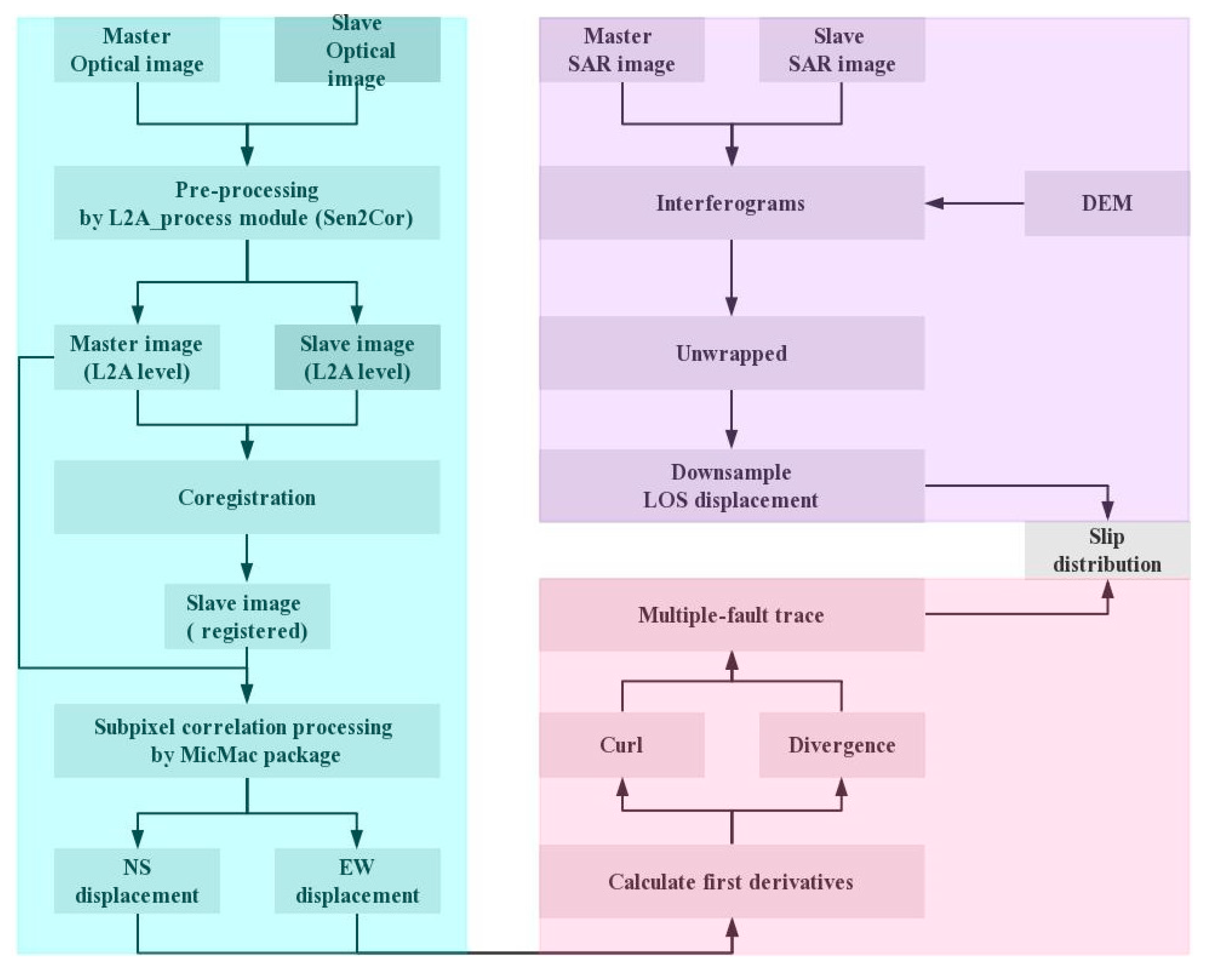
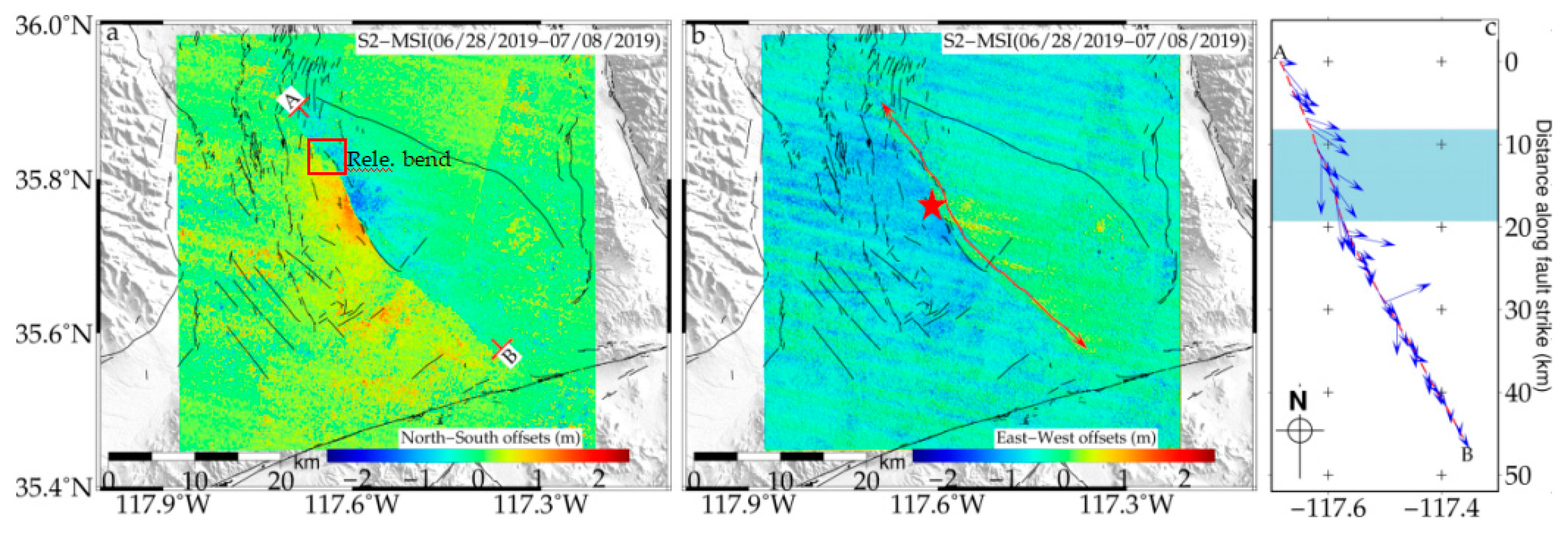
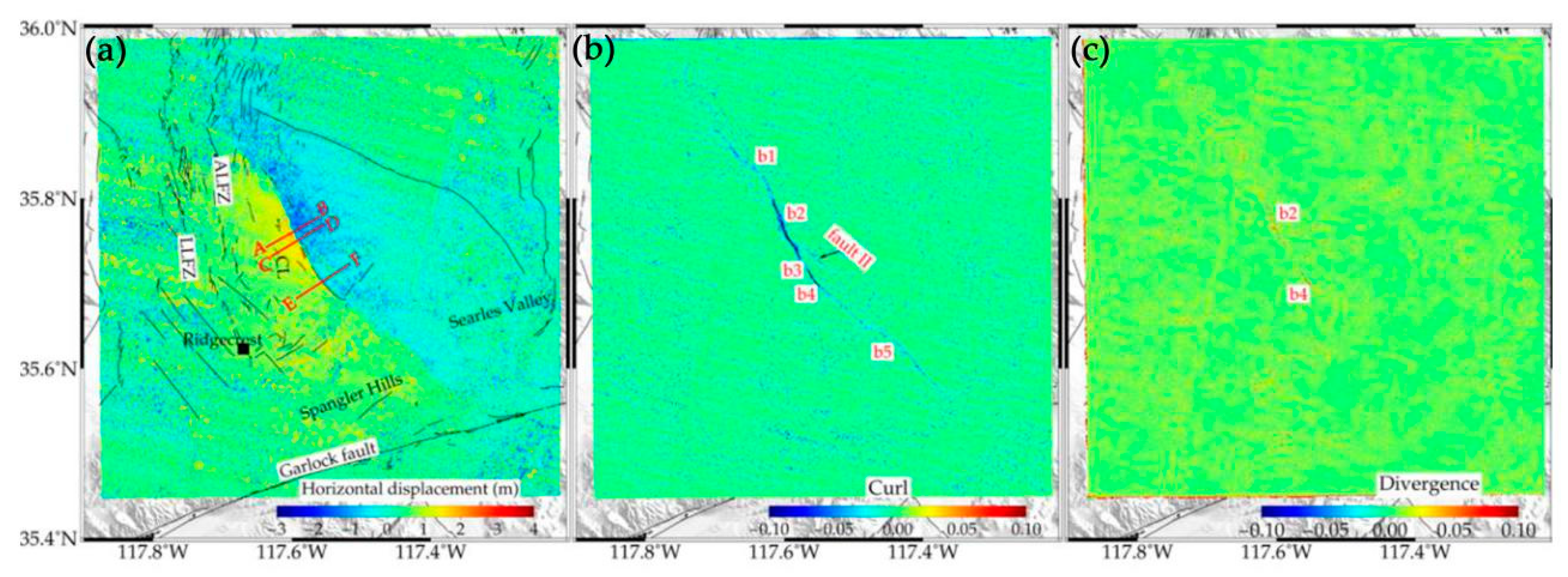
2.1. Horizontal Displacement Fields by Subpixel Correlation of Optical Images

We used the Sentinel-2 optical images (near-infrared band 8, spatial resolution of 10 m) and offset tracking method to reconstruct the horizontal displacement field of this earthquake sequence. Firstly, radiometric calibration and atmospheric correction were performed to the pre-earthquake (28 June 2019) and post-earthquake (8 July 2019) Level 1C images using the Sen2Cor package (developed by the European Space Agency) to obtain the Level 2A optical images [20]. Then, the obtained Sentinel-2 Level 2A data were processed by orthorectification and coregistration using COSI-corr software [21,22,23]. Finally, we calculated the EW and NS displacement components (10 m resolution) of the coseismic horizontal displacement field using the MicMac package based on the subpixel image correlation technology (correlation parameter setting: window = 1 pixel × 1 pixel, regularization term = 0.5, initial uncertainty = 2.0, merging factor = 1 pixel, correlation threshold = 0.5, gamma = 2) [24,25,26]. The MicMac package developed by the French National Geographic Institute can be used to compute the ground displacement field with an accuracy of 0.1 pixel [14]. An overview of the data processing chain is given in Figure 2.

The high-resolution horizontal displacements provide a good opportunity to study the geometrical complexities of the surface rupture caused by this earthquake sequence. The NS component (Figure 3a) indicates that these earthquakes ruptured the unmapped active faults within the LLFZ, the China Lake Basin, and western Searles Valley. The surface rupture produced by the Mw7.1 mainshock propagated in the southeast-northwest direction between A and B in Figure 3a. The horizontal displacement increased sharply near the epicenter of the Mw7.1 event, and peaked at ~4.6 m (35.75$°$ N) (Figure 3a,b). Displacement vectors were not consistent with azimuth of the rupture trace near the epicenter (Figure 3c, blue zone), and the longer-wavelength displacement vectors corresponded to increasing NS and EW displacements here. The rupture propagated northwest from the epicenter, and the azimuth of the rupture trace suddenly turned northwest and formed a major releasing bend. This part of the rupture was notably deficient, suggesting that the releasing bend blocks the strike-slip rupture. In the south of the blue zone (Figure 3c), the rupture was also characterized by an implicit rupture trace, minor horizontal displacement component, and smoother horizontal displacement gradient.

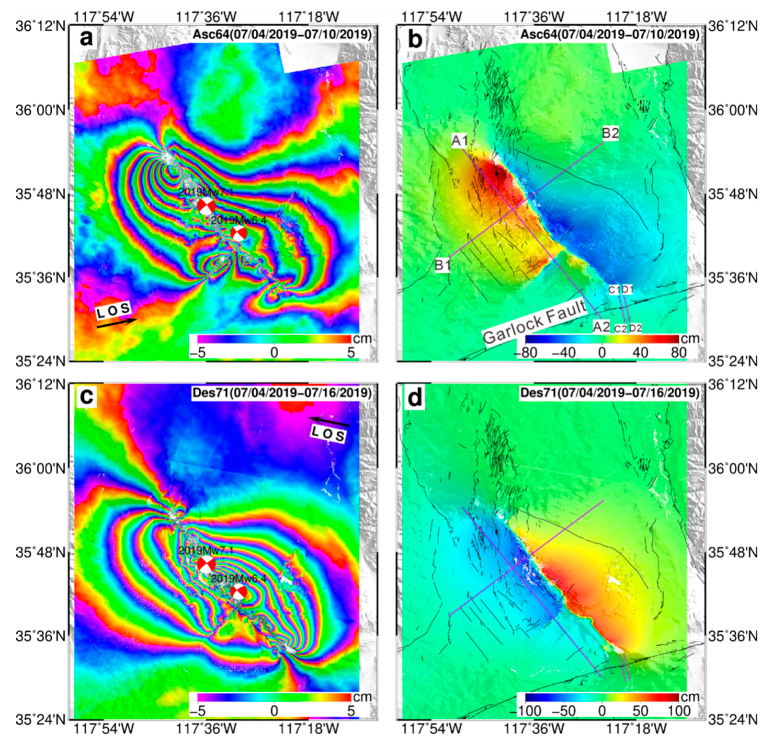
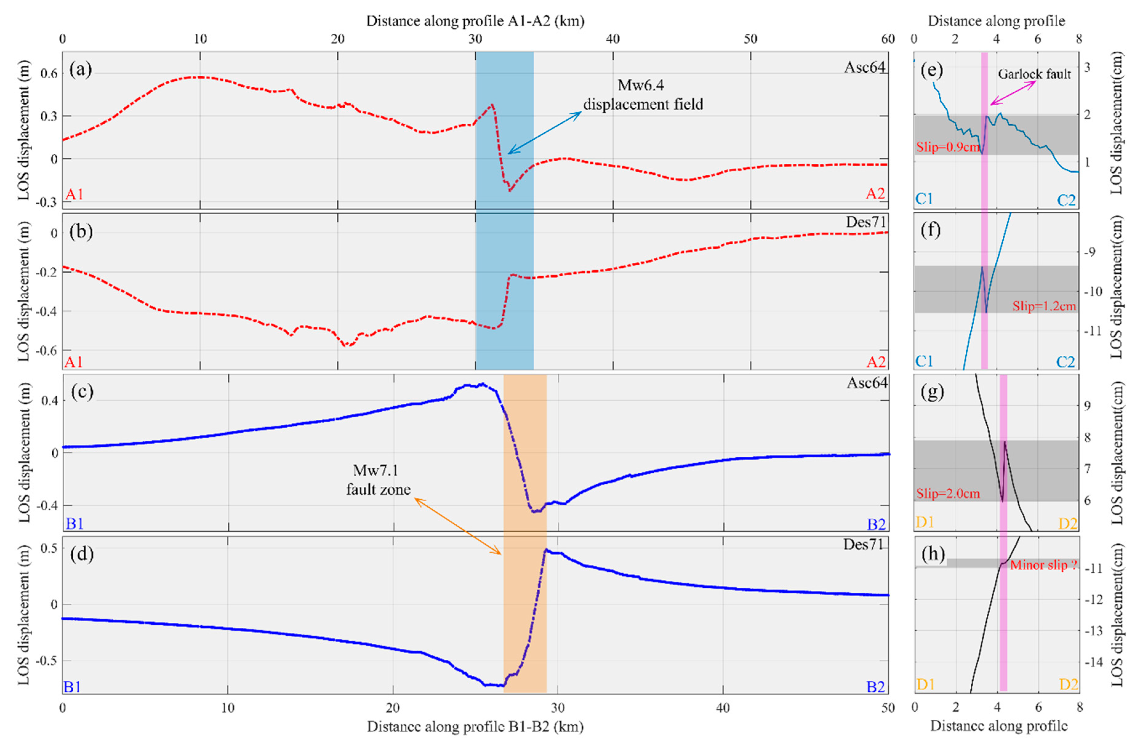
2.2. Coseismic Deformation from InSAR

We obtained the coseismic deformation fields using pre-earthquake (ascending track, 4 July 2019; descending track, 4 July 2019) and post-earthquake (ascending track, 10 July 2019; descending track, 16 July 2019) Sentinel-1 SAR images. The time resolution (revisiting period) of the Sentinel-1 ascending data is 6 days. We processed interferograms using GAMMA [27]. The topographic effects were removed using a filled 3-arc-sec (90 m) resolution Shuttle Radar Topography Mission (SRTM) digital elevation model (DEM) released by NASA [28]. In order to reduce the phase noise of the interferogram, a 10 × 2 multilooking process was applied in the range and azimuth directions during the processing. The accuracy of coregistration in the azimuth was better than 0.001 of a pixel, which can avoid phase jumps between adjacent bursts in the TOPS (Terrain Observation by Progressive Scan) data mode [29]. After the high accuracy coregistration, we filtered the interferometric phase using an adaptive spectral filtering [30] and unwrapped it utilizing the minimum cost flow (MCF) algorithm [31]. The unwrapped interferogram image was finally geocoded to the WGS-84 geographic coordinates system. The ascending and descending coseismic interferograms and the LOS deformation fields are shown in Figure 4.

The coseismic deformation fields reconstructed by Sentinel-1 data have two asymmetric lobes (Figure 4b,d) and a four-quadrant distribution pattern, which are typical for a strike-slip earthquake. The fringe patterns (Figure 4a,c) are characterized by more fringes on the western wall of the rupture, indicating that the seismogenic fault plane dips west. The maximum LOS displacement (~0.96 m) appears on the western wall of the ascending deformation field. On the west of the fault, the positive LOS displacement of the ascending deformation field (Figure 4a,c) indicates a range increase, as the satellite LOS direction (almost northward) is nearly perpendicular to the strike of the fault, which is a right-lateral strike-slip with possible uplift. In contrast, the Mw6.4 foreshock was dominated by a left-lateral strike-slip motion (blue zone shown in Figure 5).

Additionally, from the ascending and descending coseismic deformation fields derived from Sentinel-1 data, we observed the creep slip triggered by the Mw7.1 mainshock on the Garlock fault, which has not been found by geodetic measurements [32]. The across-Garlock fault displacement profiles, C1-C2 and D1-D2 in Figure 3b, indicate a more evident LOS displacement gradient alteration (Figure 5e–g) when LOS displacement profiles passed through the Garlock fault (Figure 5, purple region). However, despite the profile D1-D2 of the descending deformation field (Figure 5h) measuring only a minor fault-perpendicular LOS slip offset, the ascending profile C1-C2, the descending profile C1-C2, and the ascending profile D1-D2, respectively, measured the fault-perpendicular LOS slip offset of up to ~0.9 cm, ~1.2 cm, and ~2.0 cm. The triggered creep slip (peaking at 20 mm) extended between 117.3$°$ W and 117.5$°$ W along the Garlock fault. These results are consistent with the results got by Ross et al. [9] and Barnhart et al. [10].

3. Revealing the Geometric Complexities of Ruptures by Curl and Divergence

It is hard to investigate the geometric features of the Mw7.1 rupture utilizing only the horizontal displacement components, due to the indistinct rupture trace. Therefore, we introduced curl ω and divergence $\mathsf{\delta }$ from the NS and EW displacement components to analyze the surface deformation patterns, including the near-fault deformations where SAR images usually decorrelate. Curl ω delineates the fault trace clearly and conforms to the right-hand rule. Negative ω corresponds to clockwise rotation. Hence, negative ω at the fault trace is equivalent to right-lateral strike-slip rupture [15]. Positive divergence $\mathsf{\delta }$ is nicely consistent with the opening cracks in the uplifted region (net extension) [26]. Curl ω and divergence $\mathsf{\delta }$ are computed by the following functions:

$$\mathsf{\omega }={\left(\nabla \times \overrightarrow{F}\right)}_z=\frac{\partial v}{\partial x}-\frac{\partial u}{\partial y}$$

(1)

$$\delta ={\nabla }_h·\overrightarrow{F}=\frac{\partial u}{\partial x}+\frac{\partial v}{\partial y}$$

(2)

where $\overrightarrow{F}$ is the displacement field; u and v are the EW and NS displacement components from Sentinel-2 optical images, respectively; x is the east-west direction (E); and y is the north-south direction (N).

We found some interesting surface deformation patterns at these faults from curl ω and divergence δ (Figure 6b,c). A typical scenario of the distributed rupture (a zone width of distributed cracks) was shown in the horizontal displacement profile (Figure 7a), curl ω profile (Figure 7d), and divergence δ profile (Figure 7g), where the surface deformation distributes within the surface rupture zone (several hundred meters). The curl ω and divergence δ profiles vary seriously (from positive to negative) within the distributed rupture zone, indicating that the surface deformation is accommodated in the extensional and compressional cracks of the shallow surface without any detectable displacement on the fault. Figure 7b,e,h present an example of the second scenario where the surface slip is entirely localized on the fault (a linear, single rupture trace by visual analysis on curl field). Curl ω and divergence δ sharply increase from zero to the maximum within a very narrow zone. At the fault, the negative curl ω peaking at −0.045 corresponds to the right-lateral strike-slip motion and the positive divergence δ reaching 0.044 is also consistent with extension that occurred at the main fault locally. In addition, cross-fault profile EF shows there is another fault II (Figure 7c,f,i). The horizontal displacement swath profile EF (Figure 7c) shows the far-field slip offset of 1.92 m, near-field slip offset of 1.54 m (24% smaller than the far-field slip offset), and a slip of ~0.49 m at fault II. The off-fault deformation, which means that earthquake deformation is not concentrated on the fault, is related to several factors, such as the immaturity of the fault and the type of material at the surface through which the fault cuts. Fault II is dominated by the right-lateral strike-slip motion and ruptures 6 km with a striking of 311.7$°$ (~10° anti-clockwise rotation compared with the main rupture), with the mean slip offset of 0.5 m.

The Mw7.1 event produced a 55 km-long main fault (segments b1–b5) with the mean striking of 320.0$°$ and two secondary faults (fault I and II shown in Figure 6). The maximum horizontal slip is ~4.6 m (35.75$°$ N, at the segment b2) on the horizontal displacement field, and the result is highly consistent with the horizontal slip ~4.2 ± 0.5 m (35.78$°$ N) reported by the University Consortium for Satellite Navigation Systems and Crustal Deformation Observations (UNAVCO). To investigate the geometric complexities and rupture kinematics of the multiple faults in the Mw7.1 event, those faults were divided into five segments (b1–b5, Figure 6) according to the geometric characteristics of the surface rupture derived from curl ω and divergence δ (

Table 1. The geometry and rupture kinematics of multiple faults derived from curl and divergence.

Segment	Orientation (°N)	Length (km)	Strike (°)	${\mathsf{\omega }}_{\mathit{m}\mathit{e}\mathit{a}\mathit{n}}$	${\mathsf{\delta }}_{\mathit{m}\mathit{e}\mathit{a}\mathit{n}}$	Surface Rupture Kinematics
b1	35.7988–35.8825	16.4	315.5	−0.0157	0.0047	Right-lateral + minor vertical motion
b2	35.7305–35.7988	10.2	325.1	−0.0291	0.0116	Right-lateral + vertical motion
b3	35.7155–35.7305	2.3	—	—	—	—
b4	35.6833–35.7155	4.7	321.2	−0.0250	0.0103	Right-lateral + vertical motion
b5	35.5774–35.6833	21.1	318.3	−0.0052	≈0	Minor right-lateral
fault I	—	—	311.0	—	—	Highly discontinuous ruptures
fault II	35.7094–35.7460	6.0	311.7	−0.0184	≈0	Minor right-lateral

). The Mw7.1 event produced a 55 km-long main fault (segments b1–b5) with the mean striking of 320.0$°$ and two secondary faults (fault I and II shown in Figure 6). The maximum horizontal slip is ~4.6 m (35.75$°$ N, at the segment b2) on the horizontal displacement field, and the result is highly consistent with the horizontal slip 4.2 ± 0.5 m (35.78$°$ N) reported by UNAVCO. The negative curl ω extracted from the fault trace (Table 1) corresponds to the clockwise rotation, hence the right-lateral strike-slip motion dominated segments b1–b5 and caused the secondary faults to rupture (Table 1). Divergence δ at the fault trace (Table 1) reveals a certain near-fault vertical rupture component (extension uplift cracks) at segments b2 and b4 (Figure 4c, Table 1). We further inferred that segments b2 and b4 were dominated by the right-lateral strike-slip, with a significant vertical rupture component on the east-dipping fault. The vertical separation at segment b2 (35.73$°$ N) measured by UNAVCO is ~3.7 ± 0.2 m. The surface rupture of the Mw7.1 event terminated in front of the bedrock mountain southwest of Searles Lake (35.5774$°$ N) and only about 5 km from the central Garlock fault (Figure 8). In addition, we extracted two surface rupture traces (fault IV and V) produced by the Mw6.4 event (Figure 8) from the horizontal displacement field (Figure 6a). Fault IV and V rupture along striking 224$°$, and intersect with the main fault of the Mw7.1 event at segment b5 (Figure 8), forming a cross-faulting geometry (~90$°$). The Mw7.1 earthquake nucleated about 10 km northwest of the Mw6.4 event. The fault II trace extracted from the curl could be seen as the initial path that propagates the Mw6.4 rupture about 6 km to the northwest (Figure 8). The 2019 Ridgecrest earthquake sequence ruptured multiple faults that were unconnected on the shallow surface (Figure 8) with the Airport Lake fault zone, the China Lake basin, the Little Lake fault zone, and the western Searles Valley (Figure 8).

4. Kinematic Characteristics of the Coseismic Rupture

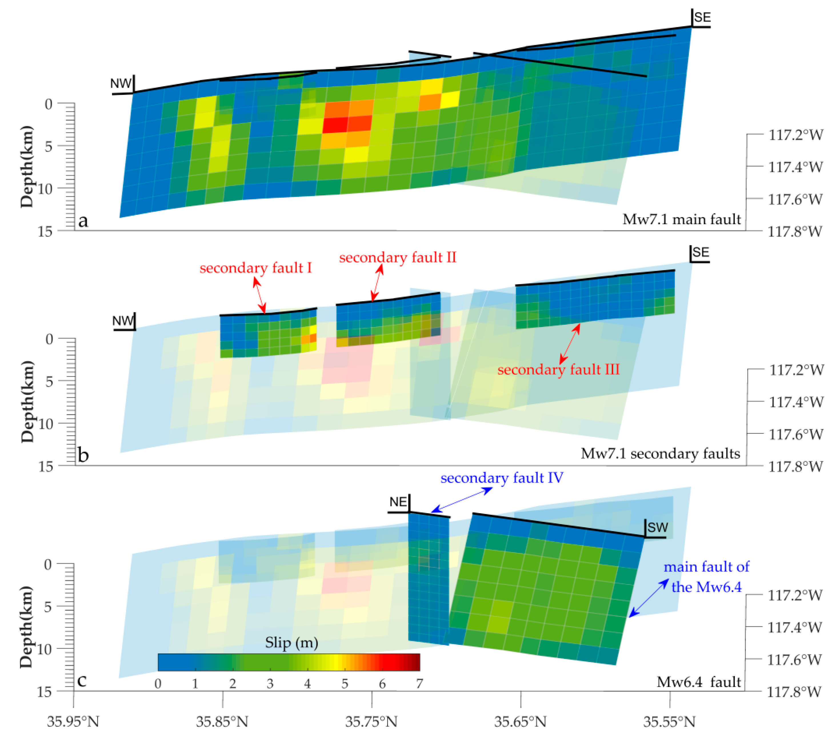
4.1. Multiple Faults Slip Distribution

To obtain the rupture process, the surface deformation fields from the Sentinel-1 ascending and descending data were utilized jointly to invert the fault slip distribution on buried fault planes. The surface deformation fields associated with this earthquake sequence were modeled as a series of dislocations buried in an elastic half space. The InSAR deformation fields were subsampled by the Quadtree algorithm to obtain a reasonable amount of data in the inversion [33]. However, by modeling the event as one occurring on a single continuous fault with varying geometric parameters, we did not obtain a well fitted fault model. Therefore, we fitted InSAR observations with a more spatially complex model of multiple-fault planes and slightly adjusted the surface rupture trace extracted from the horizontal displacement fields, curl ω and divergence $\mathsf{\delta }$, and considered them as seismogenic fault traces. In addition, we added a 15 km-long fault plane (the secondary fault III) with a striking of 319$°$ in the western part of the Mw7.1 main fault (2 km from segment b5) [9] to improve the model fitting. Finally, we approximated the model of this earthquake sequence by six faults, which are the main faults of the Mw7.1 event, three secondary faults of the Mw 7.1 event, and two faults of the Mw6.4 event.

The geometric complexities of the surface rupture derived from the horizontal displacement fields, curl ω and divergence $\mathsf{\delta },$ allowed us to constrain the multiple-fault model in orientation, strike, and length [17]. The multiple-fault geometry shows a varying strike along the ruptures that reproduces the five segments b1–b5. For determining the fault dips, we tested the fault geometries of east dipping and west dipping, and found an east dipping of 84$°$ to constrain the Mw7.1 main fault. Fault V ruptured in the Mw6.4 event and has a dip angle of 78$°$ according to USGS. Faults I, II, and III are vertical planes with a dip of 90$°$ and depth of 5 km. Moreover, we constrained the rake angle of the multiple faults more flexibly in right-lateral (Mw7.1) and left-lateral (Mw6.4) strike-slip motion. We then determined the size of the Mw7.1 main fault plane to be 58 km × 15 km and discretized it into 29 subfaults in the strike direction and 8 subfaults in the dip direction. The size of each subfault is 2 km × 2 km. The multiple-fault model includes the fault V plane (18 km × 15 km), which is discretized into 72 subfaults (2 km × 2 km), and the secondary fault planes, which are discretized into a series of subfaults (1 km × 1 km). Based on the Okada elastic half-space homogeneous model [34], we utilized the steepest descent method (SDM) to evaluate the optimal geometric parameters of the seismogenic faults and calculated the multiple-fault slip distribution (Figure 9) [35]. The predicted displacements from our multiple-fault slip distribution fit the observations well (Figure 10). The RMS of the misfits were ~0.15 m and ~0.28 m for ascending and descending deformations, respectively.

Moment tensor resolutions for the Mw6.4 foreshock are strike = 224$°$, dip = 78$°$, and rake = $5°$ for the left-lateral event and those of the Mw7.1 main shock are strike = 320$°$, dip = 81$°$, and rake = $-174°$ for right-lateral event. Our results indicate that the Mw7.1 mainshock was dominated by a right-lateral strike-slip with a maximum strike-slip of ~5.8 m near the hypocenter and accompanied by a significant dip-slip component peaking at ~1.8 m on an east-dipping fault (Figure 11a, segment b2 in Figure 6). The main fault slip distribution of the Mw7.1 event indicates that coseismic slip was concentrated in the upper crust, shallower than 10 km, and the maximum rupture occurred at a depth between 4 and 8 km (Figure 9a). The total seismic moment is 5.18 $\times {10}^{19}\mathrm{N}·\mathrm{m}$, which is equivalent to Mw7.12. In addition, the derived multiple faults model of the Mw7.1 mainshock contains three secondary faults, which are fault I located on the northwest of the epicenter (Figure 11g, releasing bend shown in the Figure 2); fault II with the strike of 310$°$, length of 10 km, and maximum slip 4 m distributed between the Mw7.1 and the Mw6.4 epicenter (Figure 11h); and fault III (Figure 11i) with a length of 15 km, strike of 319$°,$ and the slip peaking at 2 m west of the Mw7.1 main fault (distance surface rupture b5 of 2 km). The fault of the Mw 6.4 event slipped at a greater depth (2–14 km deep), with the maximum strike-slip of ~3.9 m rupturing at the depth of 12 km (Figure 9c). The strike-slip (Figure 11e) and dip-slip (Figure 11f) components indicate that the Mw6.4 event’s ruptured minute dip-slip was dominated by pure left-lateral strike-slip with a strike of 224$°$ and rake of 5$°$. In contrast, the fault IV of the Mw6.4 event (Figure 11j) ruptured at a shallower depth (2–7.5 km), with the maximum slip of ~2 m.

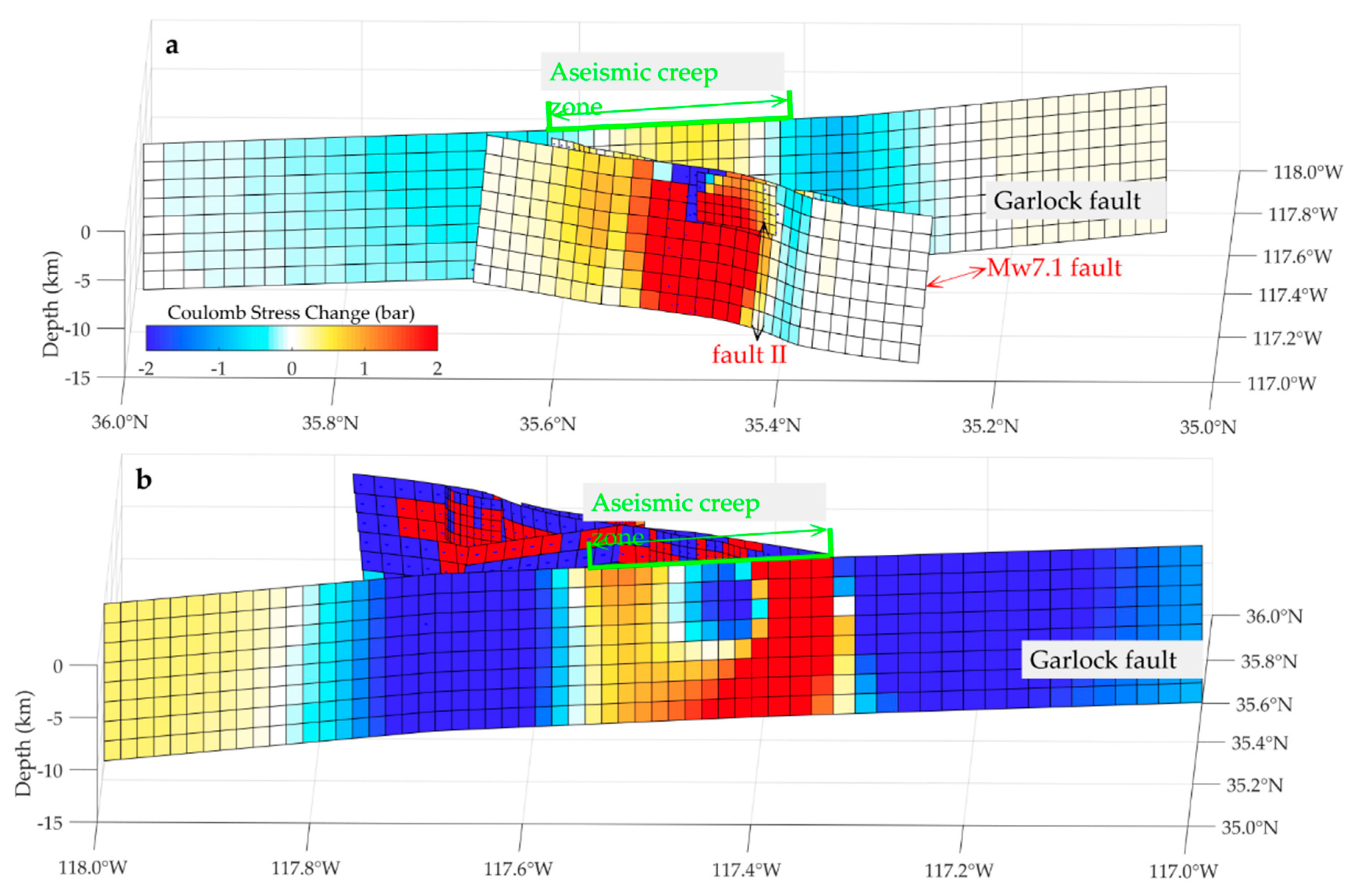
4.2. Static Coulomb Stress Changes

The coseismic rupture of faults will inevitably cause stress volume change and redistribution in the surrounding region, which affects the spatial-temporal distribution of the subsequent earthquakes [36,37,38]. Therefore, we investigated the static stress changes on the multiple-fault planes by the slip distribution model to understand the rupture processes of the Mw7.1 mainshock encouraged by the foreshock sequence, and further analyzed whether the Garlock left-lateral fault triggered shallow folding. The static Coulomb stress changes on multiple-fault planes were calculated by the Coulomb3.3 software [39,40,41]. For simplicity, we only concentrated on the triggering relationship between the Mw6.4 foreshock and the Mw7.1 mainshock, so the earthquakes between these two events were not considered. We set a fixed static coefficient of friction of 0.4, which is a typical value of inland strike slip faults. The shear modulus and Poisson’s ratio were assumed as 33 GPa and 0.25, respectively [42]. We then calculated the static Coulomb stress changes of each subfault to track the stress changes induced by the Mw6.4 foreshock on the Mw7.1 fault plane and the Garlock fault plane, and these earthquakes on the Garlock fault plane.

The Coulomb stress change model indicates that the Mw6.4 foreshock triggered the Mw7.1 mainshock and increased the Coulomb stress (0.5–1 bar) in the nucleation zone but decreased the Coulomb stress (−2 bar) in the main fault (Figure 8, segment b3 and b4) of the Mw7.1 event, leading to slight unclamping of the fault. Furthermore, the Coulomb stress loading is up to 0.5–2.0 bar on fault II, which is located between the Mw6.4 and Mw7.1 nucleation zones. Therefore, we inferred that fault II played a significant role in the triggering process. The spatial distribution of aftershocks of the Mw6.4 event also confirms our result that all aftershocks that occurred in the area between the Mw6.4 and the Mw7.1 nucleation zone ruptured along the fault II with a strike of 321$°$ (Figure 12). We also modeled the Coulomb stress changes on the Garlock left-lateral fault induced by the Mw6.4 foreshock (Figure 12a) and the Mw7.1 mainshock (Figure 12b). A 20 km-long area with increased Coulomb stress (+0.5 bar) generated by the Mw6.4 event appeared at the Garlock fault between 117.5$°$ W and 117.3$°$ W. This area appeared again when the Mw7.1 mainshock struck. The positive Coulomb stress increased up to 1–2 bar and lead to unclamping of the Garlock fault, thereby triggering shallow aseismic folding on the Garlock fault. The Mw7.1 mainshock altered the coulomb stress of the central aseismic folding zone from positive (unclamping) to negative (clamping), resulting in slight unclamping on the fault.

5. Discussion

5.1. Multiple-Fault Slip Model

Pirtro et al. used the MAI (Multiple Aperture Interferometry) technique to reconstruct the time series of the 3-D components of the 2019 Ridgcrest earthquake [43]. Our results (NS and EW displacement) are consistent with the results of Pirtro et al. Hence, the subpixel optical image correlation technology can allow us to reconstruct the coseismic displacement (NS and EW) produced by this earthquake sequence, and further investigate multiple-fault rupture traces, which is a good method to investigate multiple-fault events. Like the 1992 Landers earthquake and the 1999 Hector Mine earthquakes, the 2019 Ridgecrest earthquake sequence ruptured along a complex fault system and triggered obvious seismic and aseismic slips on multiple intersecting faults (Figure 8). In this study, we modeled the Mw6.4 left-lateral foreshock and the Mw7.1 right-lateral mainshock on two orthogonal fault structures (Figure 8 and Figure 9). Cross-fault ruptures have been very well researched, such as the 1987 Superstition Hills earthquake sequence, the 1992 Big Bears and Landers earthquakes, the 2010–2011 Darfield, New Zealand earthquake sequence [19], the 2010 Haiti earthquake, and the 2012 Sumatra earthquake [44]. For instance, the 2012 Sumatra earthquake ruptured along four faults with different geometry parameters. It is a struggle to investigate the fault traces, geometry parameters, and near-field rupture patterns of these faults only using seismic data and geodetic (GPS) observations. We can investigate the multiple faults ruptures and intersecting faults utilizing space geodesy techonolgy (InSAR and optical image correlation). The surface displacements derived from Sentinel-2 optical images and Sentinel-1 SAR images help us understand the surface rupture kinematics and deep slip distribution produced by this earthquake sequence. The surface traces of the ruptured faults can be extracted from the surface displacement fields, curl and divergence. The geometric complexities of the multiple-fault model were well constrained by the surface rupture kinematics, and the surface rupture kinematics and deep slip distribution should be consistent with each other, so then reducing uncertainties caused by the geometric parameters of the fault model in the process of inversion.

5.2. Cascading Rupture Process

According to the surface rupture kinematics and multiple-fault slip model, the Mw6.4 event and its aftershocks triggered the Mw7.1 earthquake. The rupture process of the earthquake sequence could be a cascading rupture rather than a single continuous rupture propagating along multiple faults [45,46,47,48]. Fault II (Figure 8) had a major influence on the cascading rupture process, and had a promotional effect on the dynamic process of the Mw6.4 foreshock, which indirectly triggered the Mw7.1 mainshock. This earthquake sequence provides a value opportunity to understand the cascading rupture model. In a cascading rupture process, the geometric complexities of the cross-faulting ruptures within a fault zone have a major influence on the earthquake rupture process, because there are many potential pathways (such as the Mw7.1 secondary fault II) to sustain the rupture propagation. This earthquake sequence demonstrated the cascading rupture process again, in which multiple highly distributed faults can cascade to produce a greater magnitude earthquake, and the more ruptures that cascade, the more faults will be produced by the coseismic ruptures. The Mw7.1 event ruptured multiple immature faults distributed within the southwest opening of Searles Valley and the China Lake basin. These immature faults may not be connected at a shallow depth, but they are physically connected at greater depths, at least partly. The cascading rupture process may accelerate the development of those faults and make them connected.

6. Conclusions

The 2019 Ridgecrest, California earthquake sequence ruptured along a complex fault system, which triggered obvious seismic and aseismic slip on multiple intersecting faults. Using the surface displacement derived from the Seninel-2 optical images and Sentinel-1 SAR data, and by introducing curl and divergence, we investigated the localized and distributed surface deformation patterns. The results show that a maximum surface slip of ~4.6 m, mean strike of 320$°$, and a 55 km-long surface rupture zone were produced by the Mw7.1 event. The Mw6.4 foreshock and the Mw7.1 mainshock ruptured multiple faults, and the main faults of these two events intersected each other at ~90$°$ in a cross-faulting geometry. The results inferred from geodetic observations are consistent with the rupture processes of this earthquake, which featured a complicated cascading rupture rather than a single continuous rupture propagating along multiple faults. The multiple immature faults ruptured by this earthquake sequence may be connected together at depth. Due to the rupture at shallow surfaces in this cascading rupture of the event, these immature faults became connected at a shallower depth and will continue to develop at the next seismic cycle by a connected right-lateral fault. Moreover, this earthquake sequence triggered a 20 km-long shallow aseismic folding zone on the central Garlock left-lateral fault (117.3° W–117.5° W). Further investigations on the Garlock fault by geologic and geodetic observations will be significant for understanding its contributions to seismic hazard in the Eastern California shear zone.

References

1. Mw 6.4—11 km Southwest of Searles Valley, California 2019/07/04 17:33:49 (UTC). U.S. Geological Survey. 2019. Available online: https://earthquake.usgs.gov/earthquakes/eventpage/ci38443183/executive (accessed on 4 July 2019).
2. Mw 7.1—2019 Ridgecrest Earthquake Sequence 2019/07/06 03:19:53 (UTC). U.S. Geological Survey. 2019. Available online: https://earthquake.usgs.gov/earthquakes/eventpage/ci38457511/executive (accessed on 6 July 2019).
3. Mw 5.4—16 km West of Searles Valley, California 2019/07/05 11:07:53 (UTC). U.S. Geological Survey. 2019. Available online: https://earthquake.usgs.gov/earthquakes/eventpage/ci38450263/executive (accessed on 5 July 2019).
4. Jones, L.E.; Hough, S.E. Analysis of broadband records from the 28 June 1992 Big Bear earthquake: Evidence of a multiple-event source. Bull. Seismol. Soc. Am. 1995, 85, 688–704. [Google Scholar]
5. Rymer, M.J. The Hector Mine, California, Earthquake of 16 October 1999: Introduction to the Special Issue. Bull. Seismol. Soc. Am. 2002, 92, 1147–1153. [Google Scholar] [CrossRef]
6. Jennings, C.W.; Bryant, W.A. Fault activity map of California, California Division of Mines and Geology, Geologic Data Map No. 6. Calif. Geol. Surv. 2010. [Google Scholar]
7. Hudnut, K.W.; Seeber, L.; Pacheco, J. Cross-fault triggering in the November 1987 Superstition Hills Earthquake Sequence, southern California. Geophys. Res. Lett. 1989, 16, 199–202. [Google Scholar] [CrossRef]
8. Larsen, S.; Reilinger, R.; Neugebauer, H.; Strange, W. GPS measurements of deformation associated with the 1987 Superstition Hills earthquake: Evidence for conjugate faulting. J. Geophys. Res. Solid Earth 1992, 97, 4885–4902. [Google Scholar] [CrossRef]
9. Ross, Z.E.; Idini, B.; Jia, Z.; Stephenson, O.L.; Zhong, M.; Wang, X.; Zhan, Z.; Simons, M.; Fielding, E.J.; Yun, S.-H.; et al. Hierarchical interlocked orthogonal faulting in the 2019 Ridgecrest earthquake sequence. Science 2019, 366, 346–351. [Google Scholar] [CrossRef] [Green Version]
10. Barnhart, W.D.; Hayes, G.P.; Gold, R.D. The July 2019 Ridgecrest, California Earthquake Sequence: Kinematics of Slip and Stressing in Cross-Fault Ruptures. Geophys. Res. Lett. 2019, 46, 11859–11867. [Google Scholar] [CrossRef]
11. Nieto-Samaniego, A.F.; Alaniz-Alvarez, S.A. Influence of the structural framework on the origin of multiple fault patterns. J. Struct. Geol. 1995, 17, 1571–1577. [Google Scholar] [CrossRef]
12. Massonnet, D.; Rossi, M.; Carmona, C.; Adragna, F.; Peltzer, G.; Feigl, K.; Rabaute, T. The displacement field of the Landers earthquake mapped by radar interferometry. Nature 1993, 364, 138–142. [Google Scholar] [CrossRef]
13. Binet, R.; Bollinger, L. Horizontal Co-seismic deformation of the 2003 Bam (Iran) earthquake measured from SPOT-5 THR satellite imagery. Geophys. Res. Lett. 2005, 32, 287–294. [Google Scholar] [CrossRef]
14. Vallage, A.; Klinger, Y.; Grandin, R.; Bhat, H.S.; Pierrot-Deseilligny, M. Inelastic surface deformation during the 2013 Mw 7.7 Balochistan, Pakistan, earthquake. Geology 2015, 43, 1079–1082. [Google Scholar]
15. Zhou, Y.; Parsons, B.E.; Walker, R.T. Characterizing complex surface ruptures in the 2013 Mw 7.7 Balochistan earthquake using three-dimensional displacements. J. Geophys. Res. Solid Earth 2018, 123, 10191–10211. [Google Scholar] [CrossRef] [Green Version]
16. Gold, R.D.; Reitman, N.G.; Briggs, R.W.; Barnhart, W.D.; Hayes, G.P.; Wilson, E. On- and off-fault deformation associated with the September 2013 Mw7.7 Balochistan earthquake: Implications for geologic slip rate measurements. Tectonophysics 2015, 660, 65–78. [Google Scholar] [CrossRef]
17. Socquet, A.; Hollingsworth, J.; Pathier, E.; Bouchon, M. Evidence of supershear during the 2018 magnitude 7.5 Palu earthquake from space geodesy. Nat. Geosci. 2019, 12, 192–199. [Google Scholar] [CrossRef]
18. Elliott, A.J.; Fletcher, J.M.; Fielding, E.J.; Gold, P.O.; Garcia, J.J.G.; Hudnut, K.W.; Liu-Zeng, J.; Teran, O.J. Near-field deformation from the El Mayor-Cucapah earthquake revealed by differential LIDAR. Science 2012, 335, 702–705. [Google Scholar]
19. Hamling, I.J.; Hreinsdóttir, S.; Clark, K.; Elliott, J.; Liang, C.; Fielding, E.; Litchfifield, N.; Villamor, P.; Wallace, L.; Wright, T.J. Complex multifault rupture during the 2016 Mw 7.8 Kaikoura earthquake, New Zealand. Science 2017, 356, 7194. [Google Scholar] [CrossRef] [Green Version]
20. Gascon, F.; Bouzinac, C.; Thépaut, O.; Jung, M.; Francesconi, B.; Louis, J.; Lonjou, V.; Lafrance, B.; Massera, S.; Gaudel-Vacaresse, A.; et al. Copernicus Sentinel-2A calibration and products validation status. Remote Sens. 2017, 9, 584. [Google Scholar] [CrossRef] [Green Version]
21. Ayoub, F.; Leprince, S.; Avouac, J.P. Co-registration and correlation of aerial photographs for ground deformation measurements. ISPRS J. Photogramm. Remote Sens. 2009, 64, 551–560. [Google Scholar] [CrossRef]
22. Leprince, S.; Ayoub, F.; Klinger, Y.; Avouac, J.P. Co-Registration of Optically Sensed Images and Correlation (COSI-Corr): An Operational Methodology for Ground Deformation Measurements. In Proceedings of the IEEE International Geoscience and Remote Sensing Symposium IGARSS, Barcelona, Spain, 23–27 July 2007. [Google Scholar] [CrossRef] [Green Version]
23. Leprince, S.; Barbot, S.; Ayoub, F.; Avouac, J.P. Automatic and Precise Orthorectification, Coregistration, and Subpixel Correlation of Satellite Images, Application to Ground Deformation Measurements. IEEE Trans. Geosci. Remote Sens. 2007, 45, 1529–1558. [Google Scholar] [CrossRef] [Green Version]
24. Rosu, A.M.; Pierrot-Deseilligny, M.; Delorme, A.; Binet, R.; Klinger, Y. Measurement of ground displacement from optical satellite image correlation using the free open-source software MicMac. ISPRS J. Photogramm. Remote Sens. 2015, 100, 48–59. [Google Scholar] [CrossRef]
25. Rupnik, E.; Daakir, M.; Pierrot-Deseilligny, M. MicMac—A free, open-source solution for photogrammetry. Open Geospat. Data Softw. Stand. 2017, 2, 1–9. [Google Scholar] [CrossRef]
26. Galland, O.; Bertelsen, H.S.; Guldstrand, F. Application of open-source photogrammetric software MicMac for monitoring surface deformation in laboratory models. J. Geophys. Res. Solid Earth 2016, 121, 2852–2872. [Google Scholar] [CrossRef] [Green Version]
27. Werner, C.; Wegmüller, U.; Strozzi, T.; Wiesmann, A. GAMMA SAR and interferometric processing software. In Proceedings of the ERS ENVISAT Symposium, Gothenburg, Sweden, 16–20 October 2001; p. 1620. [Google Scholar]
28. Farr, T.G.; Rosen, P.A.; Caro, E.; Crippen, R.; Duren, R.; Hensley, S.; Kobrick, M.; Paller, M.; Rodriguez, E.; Roth, L.; et al. The shuttle radar topography mission. Rev. Geophys. 2007, 45, RG2004. [Google Scholar] [CrossRef] [Green Version]
29. Song, C.; Yu, C.; Li, Z.; Li, Y.; Xiao, R. Coseismic Slip Distribution of the 2019 Mw 7.5 New Ireland Earthquake from the Integration of Multiple Remote Sensing Techniques. Remote Sens. 2019, 11, 2767. [Google Scholar] [CrossRef] [Green Version]
30. Goldstein, R.M.; Werner, C.L. Radar interferogram filtering for geophysical applications. Geophys. Res. Lett. 1998, 25, 4035–4038. [Google Scholar] [CrossRef] [Green Version]
31. Werner, C.; Wegmuller, U.; Strozzi, T.; Wiesmann, A. Processing strategies for phase unwrapping for INSAR applications. Proc. Eur. Conf. Synth. Apert. Radar (EUSAR 2002) 2002, 1, 353–356. [Google Scholar]
32. Tong, X.; Sandwell, D.T.; Smith-Konter, B. High-resolution interseismic velocity data along the San Andreas fault from GPS and InSAR. J. Geophys. Res. 2013, 118, 369–389. [Google Scholar] [CrossRef] [Green Version]
33. Lohman, R.B.; Simons, M. Some thoughts on the use of InSAR data to constrain models of surface deformation: Noise structure and data downsampling. Geochem. Geophys. Geosyst. 2005, 6, 359–361. [Google Scholar] [CrossRef]
34. Okada, Y. Surface deformation due to shear and tensile faults in a half-space. Bull. Seismol. Soc. Am. 1985, 75, 1135–1154. [Google Scholar]
35. Wang, R.; Xia, Y.; Grosser, H.; Wetzel, H.U.; Kaufmann, H.; Zschau, J. The 2003 Bam (SE Iran) Earthquake: Precise Source Parameters from Satellite Radar Interferometry. Geophys. J. Int. 2004, 159, 917–922. [Google Scholar] [CrossRef] [Green Version]
36. Lin, J.; Stein, R.S. Stress triggering in thrust and subduction earthquakes and stress interaction between the southern San Andreas and nearby thrust and strike-slip faults. J. Geophys. Res. 2004, 109, B02303. [Google Scholar] [CrossRef] [Green Version]
37. Xu, C.; Wang, J.; Li, Z.; Drummond, J. Applying the Coulomb failure function with an optimally oriented plane to the 2008 Mw 7.9 Wenchuan earthquake triggering. Tectonophysics 2010, 491, 119–126. [Google Scholar] [CrossRef] [Green Version]
38. Yu, C.; Li, Z.; Chen, J.; Hu, J.-C. Small magnitude co-seismic deformation of the 2017 Mw 6.4 Nyingchi earthquake revealed by InSAR measurements with atmospheric correction. Remote Sens. 2018, 10, 684. [Google Scholar] [CrossRef] [Green Version]
39. Toda, S.; Stein, R.S.; Richards-Dinger, K.; Bozkurt, S.B. Forecasting the evolution of seismicity in southern California: Animations built on earthquake stress transfer. J. Geophys. Res. Solid Earth 2005, 110. [Google Scholar] [CrossRef]
40. Levin, S.Z.; Sammis, C.G.; Bowman, D.D. An observational test of the stress accumulation model based on seismicity preceding the 1992 Landers, CA earthquake. Tectonophysics 2006, 413, 39–52. [Google Scholar] [CrossRef]
41. Becker, T.W.; Hardebeck, J.L.; Anderson, G. Constraints on fault slip rates of the southern California plate boundary from GPS velocity and stress inversions. Geophys. J. R. Astron. Soc. 2005, 160, 634–650. [Google Scholar] [CrossRef] [Green Version]
42. Freed, A.M.; Ali, S.T.; Bürgmann, R. Evolution of stress in Southern California for the past 200 years from coseismic, postseismic and interseismic stress changes. Geophys. J. R. Astron. Soc. 2007, 169, 1164–1179. [Google Scholar] [CrossRef] [Green Version]
43. Mastro, P.; Serio, C.; Masiello, G.; Pepe, A. The MultipleAperture SAR Interferometry (MAI) Technique for the Detection of Large Ground Displacement Dynamics: An Overview. Remote Sens. 2020, 12, 1189. [Google Scholar] [CrossRef] [Green Version]
44. Fan, W.Y.; Peter, M.S. Fault interactions and triggering during the 10 January 2012 Mw7.2 Sumatra earthquake. Geophys. Res. Lett. 2016, 43, 1934–1942. [Google Scholar] [CrossRef] [Green Version]
45. Ide, S.; Aochi, H. Historical seismicity and dynamic rupture process of the 2011 Tohoku-Oki earthquake. Tectonophysics 2013, 600, 1–13. [Google Scholar] [CrossRef]
46. Grocholski, B. Forecasting cascading fault rupture. Science 2016, 351, 1039–1040. [Google Scholar] [CrossRef] [Green Version]
47. Zhang, H.; Koper, K.D.; Pankow, K.; Ge, Z. Imaging the 2016 MW 7.8 Kaikoura, New Zealand Earthquake with Teleseismic P Waves: A Cascading Rupture Across Multiple Fault. Geophys. Res. Lett. 2017, 44, 4790–4798. [Google Scholar] [CrossRef]
48. Fletcher, J.M.; Oskin, M.E.; Teran, O.J. The role of a keystone fault in triggering the complex El Mayor–Cucapah earthquake rupture. Nat. Geosci. 2016, 9, 303–307. [Google Scholar] [CrossRef]
Figure 1. Tectonic setting of the 2019 Ridgecrest earthquake sequence. (a) Spatio-temporal distribution of foreshocks and aftershocks. Two stars and beach balls mark the epicenters and focal mechanisms of the 2019 Mw7.1 Ridgecrest earthquake and the Mw6.4 Searles Valley earthquake (from the U.S. Geological Survey (USGS)), respectively. Blue and pink dots represent the spatial distribution and temporal evolution of foreshocks and aftershocks of the Mw7.1 mainshock, respectively. (b) White rectangle shows the spatial coverage of the Sentinel-1 ascending (track 64) data utilized in this study and the yellow one shows the spatial coverage of the Sentinel-1 descending (track 71) data. The green rectangle shows the spatial coverage of the Sentinel-2 optical image. Black moment tensors represent focal mechanisms of large historical events (Mw > 6.5) that occurred within southern California. ALFZ: Airport Lake fault zone; LLFZ: Little Lake fault zone; ECSZ: Eastern California shear zone; SAF: the Sande Andres fault.
Remotesensing 12 03883 g001
Figure 2. Overview of the data processing chain used in this investigation. Sen2Cor is a processor for Sentinel-2 Level 2A (L2A level) product generation and formatting. MicMac: Multi Images Correspondances par Méthodes Automatiques de Corrélation. LOS: line-of-sight. DEM: digital elevation model.
Remotesensing 12 03883 g002
Figure 3. Horizontal displacement field of the 2019 Ridgecrest earthquake sequence. (a) North-south (NS) component of the horizontal displacement derived from Sentinel-2 optical images (28 June 2019–8 July 2019). The amplitude of the displacement is negative where the motion is southward and positive where the motion is northward; (b) East-west (EW) component of the displacement field derived from Sentinel-2 optical images (28 June 2019–8 July 2019). The amplitude of displacement is negative where the motion is westward and positive where the motion is eastward. The red star indicates the epicenter of the Mw7.1 event; (c) Displacement vectors (blue arrows) determined from the profile AB of the NS and EW horizontal displacements. Red dashed line indicates the surface rupture trace of the Mw7.1 event.
Remotesensing 12 03883 g003
Figure 4. Ascending and descending coseismic interferograms (a,c) and deformation fields (b,d) of the 2019 Ridgecrest earthquake sequence. A color cycle in interferograms corresponds to a 10 cm deformation in line-of-sight (LOS) direction. Negative LOS displacement values in the deformation field suggest movement away from the satellite. LOS direction is indicated by the black arrow. Active faults are plotted as black thin lines. The purple lines in (b,d) denote the profile locations A1-A2, B1-B2, C1-C2, and D1-D2.
Remotesensing 12 03883 g004
Figure 5. Profiles of the Ridgecrest earthquake sequence. The line-of-sight (LOS) displacement profile of (a) the ascending deformation field and (b) the descending deformation field along A1-A2; The LOS displacement profile of (c) the ascending deformation field and (d) the descending deformation field along B1-B2; (eh) jointly reveal the triggered creep on the Garlock fault perpendicular to profiles C1-C2 and D1-D2.
Remotesensing 12 03883 g005
Figure 6. Curl and divergence of the surface ruptures due to the mainshock. (a) Coseismic horizontal displacement field derived from the NS and EW displacement components. Amplitude of displacement is negative for southward motion. (b) Curl ω and (c) divergence δ derived from the NS and EW displacement components. Across-fault profiles (AB, CD, and EF) reveal detailed characteristics of the surface rupture zone (both near-field and far-field). Geometrical complexities of the surface rupture contributed by the Mw7.1 event are indicated in bend b1–b5.
Remotesensing 12 03883 g006
Figure 7. Near-field and far-field measurements. (ac) Horizontal displacement measurements along profiles AB, CD, and EF (7-km-long and 200-m-wide) of Figure 5, respectively. (df) Curl profiles (AB, CD, and EF) show three peaks, corresponding to the main rupture at the site. In both cases, curl delineates the fault trace clearly, and the right-lateral strike-slip motion results in clockwise rotation at the fault and hence negative curl ω . (gi) Divergence profiles (AB, CD, and EF) reveal three positive peaks (δ > 0), corresponding to net extension at the fault.
Remotesensing 12 03883 g007
Figure 8. The surface rupture traces of the 2019 Ridgecrest earthquake sequence. Purple lines indicate the faults recorded in the U.S. Geological Survey (USGS) Quaternary Fault database (U.S. Geological Survey and California Survey, 2010) and in the 2010 Fault Activity Map of California (California Geologic Survey, 2010). Black lines indicate the surface rupture traces of the main fault and some secondary faults identified from displacement field and curl. Blue beach balls show the focal mechanisms of the large foreshock (from USGS). Red lines indicate the surface rupture traces produced by the mainshock obtained by field investigations. Green rectangles indicate the regions with the horizontal slip ~4.2 ± 0.5 m and vertical separation ~3.7 ± 0.2 m reported by the University Consortium for Satellite Navigation Systems and Crustal Deformation Observations (UNAVCO).
Remotesensing 12 03883 g008
Figure 9. The slip distribution model of the multiple faults: (a) Mw7.1 main fault, (b) Mw7.1 secondary faults, and (c) Mw6.4 main fault.
Remotesensing 12 03883 g009
Figure 10. Coseismic LOS observations from ascending Sentinel-1 interferograms (a), predictions from our slip model (b), and residuals between of them (c). Observations from descending Sentinel-1 interferograms (d), predictions from our slip model (e), and residuals between them (f).
Remotesensing 12 03883 g010
Figure 11. Slip distribution on the multiple faults. The distribution of (a) the total-slip, (b) strike-slip, and (c) dip-slip on the Mw7.1 main fault. The distribution of (d) total-slip, (e) strike-slip, and (f) dip-slip on the Mw6.4 main fault. (gj), The total-slip distribution on (g) fault I, (h) fault II, and (i) fault III of the Mw7.1 event and (j) fault IV of the Mw6.4 foreshock. Bends b1–b5 correspond to surface ruptures b1–b5 of the Mw7.1 event.
Remotesensing 12 03883 g011
Figure 12. Static Coulomb stress changes (CSC) on multiple faults due to the 2019 earthquakes. (a) CSC on the Mw7.1 faults and the Garlock fault plane caused by the Mw6.4 event; (b) CSC on the Garlock fault plane caused by the 2019 Ridgecrest earthquake sequence. The green line indicates the aseismic creep triggered by these earthquakes. Static coefficient of friction is 0.2. Positive stress change is consistent with unclamping of the faults, and a negative stress change leads to clamping of the faults.
Remotesensing 12 03883 g012