Evaluating Feature Extraction Methods with Synthetic Noise Patterns for Image-Based Modelling of Texture-Less Objects

Abstract

Image-based three-dimensional (3D) reconstruction is a process of extracting 3D information from an object or entire scene while using low-cost vision sensors. A structure-from-motion coupled with multi-view stereo (SFM-MVS) pipeline is a widely used technique that allows 3D reconstruction from a collection of unordered images. The SFM-MVS pipeline typically comprises different processing steps, including feature extraction and feature matching, which provide the basis for automatic 3D reconstruction. However, surfaces with poor visual texture (repetitive, monotone, etc.) challenge the feature extraction and matching stage and affect the quality of reconstruction. The projection of image patterns while using a video projector during the image acquisition process is a well-known technique that has been shown to be successful for such surfaces. In this study, we evaluate the performance of different feature extraction methods on texture-less surfaces with the application of synthetically generated noise patterns (images). Seven state-of-the-art feature extraction methods (HARRIS, Shi-Tomasi, MSER, SIFT, SURF, KAZE, and BRISK) are evaluated on problematic surfaces in two experimental phases. In the first phase, the 3D reconstruction of real and virtual planar surfaces evaluates image patterns while using all feature extraction methods, where the patterns with uniform histograms have the most suitable morphological features. The best performing pattern from Phase One is used in Phase Two experiments in order to recreate a polygonal model of a 3D printed object using all of the feature extraction methods. The KAZE algorithm achieved the lowest standard deviation and mean distance values of 0.0635 mm and −0.00921 mm, respectively.

1. Introduction

In recent years, structure-from-motion coupled with multi-view stereo (SFM-MVS) techniques has been a focus of research in the fields of photogrammetry (image-based three-dimensional reconstruction) and computer vision, owing to the availability of low-cost vision sensors and methods for automated image processing [1,2]. SFM-MVS has influenced various areas, such as medicine (e.g., to examine changes in muscle tissue [3]), cultural heritage (e.g., to document digital museum archives [4], and visualization of museums in a virtual environment [5,6]), criminal investigation (e.g., forensic infography [7], and inspection for concealed weapons [8]), reverse engineering (e.g., investigation of industrial components [9]), forestry and ecology [10,11], virtual and augmented reality [12,13,14], applications in the entertainment and gaming industries [15,16], as well as other fields.

SFM is a non-contact measuring technique that is used to find a set of feature points that appear in different images. The feature points can be used in order to retrieve the captured scene and estimate the position and orientation of the camera stations. By utilizing the orientation parameters, the three-dimensional (3D) coordinates of the camera stations and sparse point cloud can be estimated in 3D space. MVS techniques can then be employed to group the images that share common viewpoints and add more points to the SFM cloud [17]. However, surfaces with poor visual texture (uniform, monotone, repetitive textures, etc.) pose a problem that is related to the extraction of feature points required for the correspondence search (tie point detection) between different images. The lack of visual features results in empty holes appearing in the point clouds. Typically, features are identified using a feature detector-descriptor algorithm. Surfaces that possess strong morphological features together with high-frequency color changes enable easy and clear identification of feature points that are considered to be SFM-MVS friendly. Conversely, surfaces with uniform and monotone visual textures pose problems and affect the quality of 3D reconstruction. Therefore, texture analysis has been widely investigated in computer vision and pattern recognition applications because of its ability to extract discriminative features [18].

Accuracy, time, and cost are important factors when choosing a 3D scanning approach. When compared to other 3D scanning techniques (e.g., laser scanning and time-of-flight), photogrammetry is time efficient and cheaper, but it lacks the accuracy that is needed for a range of applications. Specifically, objects with a texture-less surface pose a challenge to the SFM-MVS pipelines due to the lack of visual features. The problem of extracting features on texture-less surfaces is often dealt with by artificially enriching surfaces with image patterns. In [3], Chang et al. proposed a multi-view image capturing system with projectors in order to monitor the deformity of a human spine to diagnose scoliosis. Because the torso surface is uniform and texture-less, synthetic image patterns were added to the surface while using video projectors before the image acquisition process. Ahmadabadian et al. implemented an automatic portable system for image acquisition with a novel projection system [19,20]. A total of 60 colored LED lights were located around a turntable to project a pattern on the object placed on the turntable. The structural resolution evaluation of the complex object resulted in an error of 0.3 mm for the system. With the application of noise function-based patterns (NFBPs), Koutsoudis et al. [21] presented a data collection variant in order to improve the reconstruction quality using a commercial software package. The performance of the NFBPs was verified on a Cycladic figurine, where the wavelet noise pattern achieved a minimum root mean square (RMS) error of 0.24 mm. Recently, Santosi et al. [22] introduced the idea of noise patterns generated from irrational numbers and random numbers of various hues. The performance evaluation of the noise patterns involved the reconstruction of an aluminum test model. The accuracy achieved for the highest-ranked pattern was 0.173 mm std. distance, and a mean distance of 0.016 mm. In our previous research [23,24,25], we have shown that the structural resolution and elements in a pattern affect the quality of reconstruction. A random dense mesh of artificial elements on a texture-less surface results in a higher accuracy when compared with a uniform and repetitive texture.

In this study, we evaluate the performance of feature extraction methods on texture-less surfaces by applying synthetic noise patterns. The patterns (images) are generated from three known sources that have been proven to be effective, namely, noise functions, irrational numbers, and random numbers. Based on the related literature previously reviewed, we assume that the arrangement and intensity values (pixels) of the pattern images have an impact on the ability of the feature extraction methods to detect and identify the feature points. The aim is to evaluate the noise patterns with different feature extraction methods while using the results of real and virtual planar surface 3D reconstruction. Additionally, the aim is to find a combination of a noise pattern and a feature extraction method that gives the highest accuracy by evaluating the reconstructed polygonal models of a texture-less object. Furthermore, we develop a MATLAB-based plug-in that encompasses state-of-the-art methods for feature extraction (HARRIS, Shi-Tomasi, MSER, SIFT, SURF, KAZE, and BRISK) and feature matching.

The remainder of this paper is organized, as follows. In Section 2, we present a brief overview of the SFM-MVS pipeline and different feature extraction methods. In Section 3, the generation of noise patterns, outline data collection, and a feature extraction and matching plug-in are described. In Section 4, we present and explain the evaluation results. We conclude the paper in Section 6 by outlining important findings.

2. Structure-from-Motion Multi-View Stereo Pipeline

2.1. Feature Extraction—Feature Detection and Description

The feature point (also called the interest point or keypoint) detection constitutes a crucial phase and it significantly affects the underlying SFM-MVS pipeline. For each image given as input to the pipeline, features are typically detected in the form of lines, edges, corners, junctions, blobs, etc. while using a so-called feature detector algorithm. Ideally, a feature detector needs to be robust and it should detect the same features across the image sequence, regardless of lighting conditions, image rotation, scale, or affine changes. For the feature detection phase in SFM pipelines, different algorithms can be used. In this paper, we present a comprehensive overview of HARRIS [26], Shi-Tomasi [27], and BRISK [28] in order to detect corner features, and SIFT [29], SURF [30], KAZE [31], and MSER [32] algorithms to detect blob features, utilizing the MATLAB Computer Vision Toolbox [33].

The feature points that were detected by feature detector algorithms (in the previous phase) are subsequently described in a process, called feature description. In this process, features are described by assigning them a distinctive identity while using logically different techniques that are based on the unique patterns possessed by their neighboring pixels. SIFT, SURF, KAZE, and BRISK feature detectors come with their designated feature descriptors, while HARRIS, Shi-Tomasi, and MSER exist individually. However, the individual feature detectors may be combined with various types of appropriate feature descriptors. Once feature points and their description are obtained, the conjugate points between different images are searched in the next step.

In the following, a brief introduction of the feature detection methods used in the experiments is presented.

2.1.1. HARRIS Corner Detector

In 1988, Harris et al. introduced a combined corner and edge detector [26] in order to improve Moravec’s corner detector. Similar to Moravec’s algorithm, the Harris Corner Detector is based on the autocorrelation, which is the sum of squared differences (SSD). Moravec’s SSD, as given by Equation (1), calculates the difference in intensities of the window shift, where $E(u,v)$ is the weighted SSD between two patches.

$$E(u,v)={\Sigma }_x{\Sigma }_y\left[w(x,y){[I(x+u,y+v)-I(x,y)]}^2\right]$$

(1)

A lower value indicates a flat region in the image, while a higher value indicates that a corner is present. When compared to Moravec’s method, the Harris Corner Detector has the advantage that instead of shifting patches for every 45-degree angle, it directly considers the differential of the corner score with respect to the direction, which has been proved to distinguish between edges and corners more accurately. Hence, the term $I(x+u,y+v)$ is approximated using the Taylor expansion truncated to the first order. After some calculation, Equation (1) can be written as

$$E(u,v)\approx {\Sigma }_x{\Sigma }_y\left[w(x,y){[I(x,y)+u{I}_x+v{I}_y-I(x,y)]}^2\right]$$

(2)

where $I_x$ and $I_y$ are partial derivatives of I in terms of the x- and y- axis, respectively. This approximation also greatly reduces the calculation complexity. Further, Harris reformulated the algorithm to benefit from the variation of E(x,y) with respect to the direction of the shift. Therefore, Equation (2) can be rewritten as

$$E(u,v)=\left[\begin{array}{cc}u& v\end{array}\right]M\left[\begin{array}{c}u\\ v\end{array}\right]$$

(3)

where the Harris matrix M is

$$M=\sum _x\sum _{y}w\left(x,y\right)\left[\begin{array}{cc}{I}_x{I}_x& I_x{I}_y\\ I_x{I}_y& I_y{I}_y\end{array}\right]$$

(4)

Next, a score, R, which is based on the eigenvalues of the Harris matrix M, is introduced in Equation (5), where the magnitudes determine whether a window contains a corner, and the eigenvalues are replaced by a matrix determinant and trace.

$$R={\lambda }_1{\lambda }_2-\kappa {({\lambda }_1+{\lambda }_2)}^2=det\left(M\right)-\kappa trac{e}^2\left(M\right)$$

(5)

2.1.2. Shi-Tomasi Method

In [27,34], Tomasi et al. proposed a method that is very similar to the Harris Corner Detector for tracking corners between consecutive frames of a video. The mathematical foundation is very similar to the formerly discussed method, except for the score criteria (R is the Harris score), which has been proved to be better than the original method. In Equation (6), the smallest eigenvalues of the Harris matrix M determine a corner.

$$R=min({\lambda }_1,{\lambda }_2)$$

(6)

If R is greater than a certain threshold, then it can be marked as a corner.

2.1.3. MSER

In [32], Mates et al. proposed the concept of maximally stable extremal regions (MSER), which can be distinguished in an image by the extremal property of the intensity function in the region and on its outer boundary. These extremal regions possess highly desirable properties, including continuous geometric transformation, and they are invariant to affine intensity changes, forming a stable local detector. MSERs are also detected at different scale levels and, since no smoothing is applied, large structures can be easily detected.

2.1.4. SIFT

The scale-invariant feature transform (SIFT) was first introduced by Lowe in 2004 [29]. Since then, many variations have been presented, such as SiftGPU [35]. The SIFT feature detector operates by finding the difference of Gaussians (DoG), which is an approximation of the Laplacian of the Gaussian (LoG). Once the DoG is found, the feature points are detected by searching the local extrema at various scale levels of the image. This property causes the detector to find the maximum number of features. Next, a refinement process eliminates some features if their intensity level is below a certain threshold. The SIFT descriptor works by taking a 16 × 16 neighborhood around the detected features and it further divides the region into 16 sub-blocks. The SIFT descriptor contains 128 bin values and it is represented as a vector. Equation (7) shows the convolution of the difference between two Gaussians that were computed at different scales with image $I(x,y)$.

$$D\left(x,y,\sigma \right)=(G\left(x,y,k\sigma \right)-G\left(x,y,\sigma \right)\ast I(x,y))$$

(7)

where G represents a Gaussian function.

2.1.5. SURF

The speeded up robust features (SURF) algorithm was introduced by Bay et al. in 2008 [30], which also relies upon Gaussian approximation of an image at many scales. The SURF detector uses an approximation of the determinant of the Hessian matrix with integral images in order to improve the feature detection speed. The SURF descriptor is based on the distribution of Haar wavelet responses around each detected feature point. A standard SURF descriptor contains 64 bin values; however, it can be extended to 128 bin values to cater to larger viewport changes. The Hessian matrix $‘‘\mathcal{H}"$ is assembled, as expressed in Equation (8) at point $\mathcal{P}$ = $(x,y)$ and scale $\sigma$

$$\mathcal{H}\left(x,\sigma \right)=\left[\begin{array}{cc}{L}_{xx}(\mathcal{P},\sigma )& L_{xy}(\mathcal{P},\sigma )\\ L_{xy}(\mathcal{P},\sigma )& L_{yy}(\mathcal{P},\sigma )\end{array}\right]$$

(8)

where $L_{xx}(P,\sigma )$ is the convolution of the Gaussian second-order derivative with image I at point $\mathcal{P}$, and similarly for $L_{xy}(\mathcal{P},\sigma )$ and $L_{yy}(\mathcal{P},\sigma )$.

2.1.6. BRISK

Leutenegger et al. introduced the binary robust invariant scalable keypoint (BRISK) method primarily for real-time applications [28]. The BRISK algorithm works by creating a scale-space pyramid, which is referred to as octaves and intra-octaves, and it finds corners using the AGAST algorithm. Next, it computes the FAST score for each scale-space while searching for maxima to reduce redundancy. The BRISK descriptor archives rotation and orientation invariance by identifying the local gradient for each corner. For the illumination invariance, it compares the pixel-to-pixel intensity, obtains the results by testing the brightness, and a binary string of the descriptor is constructed.

2.1.7. KAZE

In 2012, Alcantarilla et al. proposed the KAZE feature detector based on a nonlinear scale-space through nonlinear diffusion filtering [31]. In this way, blurring in an image becomes locally adaptive, which reduces noise but retains the boundaries of the objects in the image data. The KAZE algorithm is based on the scale-normalized determinant of the Hessian matrix computed through nonlinear scale-space at multiple levels. The maxima of the Hessian response are found as features of interest. The KAZE descriptor achieves rotation invariance by finding the dominant orientation in a circular region that is centered at the location of the feature point. Equation (9) shows the standard nonlinear diffusion formula.

$$\frac{\partial L}{\partial t}=div(c\left(x,y,t\right).\nabla L)$$

(9)

where c is the conductivity function, $‘‘div"$ is divergence, ∇ is the gradient operator, and L is image luminance.

2.2. Feature Matching

The feature points obtained through the feature extraction process are used in order to find image regions that share common parts of the scene. If an image pair finds a set of feature points that are present in both images, then it is possible to state that those images share a common part of the scene. In a similar fashion, images in a sequence are matched with all other images in order to find a set of correspondences. Different matching methods (FLANN and Brute-Force) and strategies (nearest neighbor distance ratio and threshold-based matching) can be adopted to find matches between images [36].

Because matches found can be contaminated by outliers, it is mandatory to use robust estimation techniques for accurate fitting of the transformation model. Depending on the configuration of the device used in the image acquisition process, different probabilistic methods, such as random sample consensus (RANSAC) [37] and progressive sample consensus (PROSAC) [38], are used to remove outliers from the matched features. These methods provide a transformation function (homography or fundamental matrix) that acts as a relative orientation backbone and gives perspective transforms between image pairs of a scene.

2.3. Bundle Adjustment

The position and rotation of the camera stations in 3D space are estimated after finding the set of correspondences between image pairs. The associated process needs to calculate the external orientation or extrinsic parameters of the camera [39]. The bundle adjustment (BA) technique estimates the external orientation parameters with the help of the image coordinates and collinearity equations. Mathematically speaking, BA is a process of optimizing the sum of the reprojection error through nonlinear least squares and estimating the 3D coordinates of the points on the image and camera parameters (potentially both intrinsic and extrinsic parameters). Therefore, BA is sometimes referred to as “auto-calibration” or “self-calibration”. Given a vector of camera parameters, x, and reprojection errors, $f\left(x\right)=\left[f_1\left(x\right),\dots ,f_k\left(x\right)\right]$, the nonlinear least squares optimization problem can be expressed as

$$x^{\ast }=argmi{n}_x\sum _{i=1}^k{∥\begin{array}{c}{f}_i\left(x\right)\end{array}∥}^2$$

(10)

The Levenberg–Marquardt (LM) algorithm, which is also known as damped least-squares, is the most renowned algorithm used for BA. It operates by solving the least-squares method for the nonlinear case. The output of the BA is a sparse cloud of points with the pose of the camera stations.

2.4. Dense Cloud Reconstruction

Using the location of camera stations and sparse point clouds as initial information from the SFM, MVS vision techniques produce additional points in the SFM cloud. Clustering views for MVS (CMVS) [40] and patch-based MVS (PMVS) [41] are popular techniques for MVS vision. In dense reconstruction, camera stations that observe common parts of the scene are first clustered by CMVS in order to improve computing efficiency, and then PMVS contributes more points to the sparse cloud through the process of feature matching, patch expansion, and patch filtering.

2.5. Mesh Reconstruction

Once the dense cloud of the object is reconstructed, the 3D points can be connected as a mesh to form a more complete model of the object, which is known as a polygonal model. Poisson surface reconstruction is a common approach that can build a smooth 3D polygonal model by efficiently removing noise on the surface and flexibly determining the mesh dimensions [42].

3. Proposed Methodology

As explained above, the morphological features of the object surfaces to be reconstructed are very important. Poorly textured and repetitive structures may lead to an erroneous or incomplete representation of the original scene due to a lack of visual features. The problem is that, to function properly, a feature detector requires a number of distinct features; if there is nothing on the surface, then it does not work. In order to avoid this dilemma, the examined surface must be, in an artificial way, enriched by projecting synthetic image patterns, adding a very dense network of the interest points. Therefore, in this study, we investigate which feature detection method is the most suitable, where algorithms must operate under very specific conditions.

3.1. Pattern Generation

For the purpose of this research, we have chosen seven different types of noise patterns that are generated from three different sources, including noise functions, irrational numbers, and random number generators. The first three patterns (Salt & Pepper, Gauss, and Speckle) categorized as NFBPs were produced while using the imnoise MATLAB function. NFBPs are generated through deterministic algorithms that are known for their pseudo-randomness and ability to provide irregularities. The second category of patterns is based on the digits of the irrational numbers $\pi$ = 3.14…, the golden ratio $\varphi$ = 1.61…, and Euler’s number e = 2.71...; hence, they are known as irrational number patterns (INPs). The digits for the INPs were obtained while using “y-cruncher” software, which is a number-crunching program. These numbers were chosen because of their unique feature, the randomness of digits after the decimal. The last two patterns (Random and Random Eq) are categorized as random number patterns (RNPs) because of the same generation method. The random numbers for these patterns were generated while using the MATLAB function randi, which is a pseudo-random number generator.

For the INPs, the strings of digits obtained from the y-cruncher software consist of numbers ranging from 0 to 9, where the digits from 1 to 8 represent particular levels of gray. Digits 0 and 9 represent black and white colors, respectively. The strings of digits of each INP were equalized in the range of 0–255, resulting in a uniform intensity histogram. Similarly, the Random Eq pattern was produced by applying the histogram equalization to the random pattern in order to form a uniform intensity histogram. The number of digits required for both INPs and RNPs depends on the resolution of the projecting device. Therefore, a total of 786,432 digits were generated to match the resolution (1024 × 768 pixels) of the native projection system. Once a sufficient number of digits were calculated, the bitmap representation (synthetic images) of the patterns was generated while using MATLAB. Figure 1 shows the partial bitmaps and intensity histograms of the generated synthetic images.

3.2. Experiment Setup and 3D Reconstruction Outline

The experiment was performed in two phases. In the first phase, the 3D digitization of a planar surface was accomplished in order to examine the performance of noise patterns using various feature extraction methods. The planar surface reconstruction assessment led to the selection of the best performing pattern that was used for the reconstruction of a complex featureless 3D object in the second phase of the experiment.

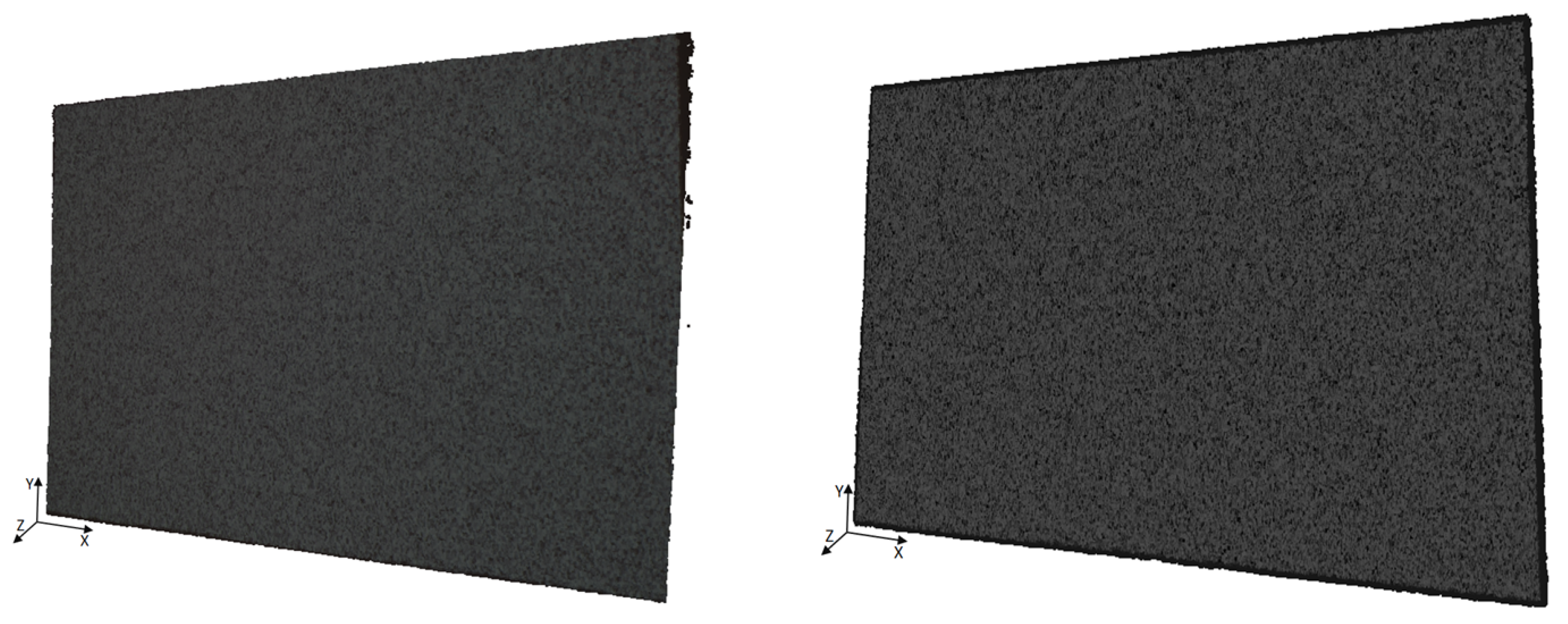
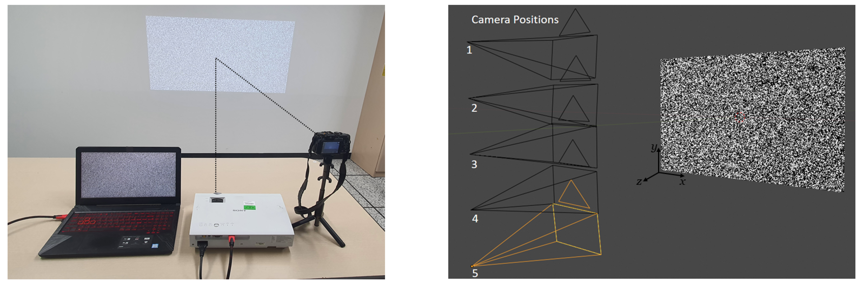
3.2.1. Phase One: Planar Surface Data Collection

A monochromatic planar surface is a worst-case scenario for an SFM-MVS pipeline, because it contains no distinctive morphological features required by the feature extraction process. This characteristic makes it useful for the evaluation of synthetically generated images (patterns) as well as feature extraction methods with several other benefits. First, the experimental setup is easy to adjust, and no special equipment is required. Second, there is no occlusion problem during the image acquisition process and noise patterns are visible in all images. Third, only a minimum number of images are required, thus reducing the time for 3D reconstruction. Finally, for a planar surface 3D reconstruction, experiments can be performed while using two approaches, real and virtual.

For real planar surface 3D reconstruction, a Sony VPL-DX120 video projector (resolution of 1024 × 768 pixels) along with a Canon PowerShot G11 digital camera (10 megapixels, 6–30 mm lens) were used. A plane white wall surface was considered to be the sample material (Figure 2 (left)). During the image capturing process, the projector was positioned on a table at a throw distance of 3 m, providing the size of the projected image of 2.02 m × 1.51 m. Next to the projector, a camera that was mounted on a tripod was positioned in such a way that the optical axis of the camera and projector remained convergent. For all of the projections of noise patterns, a total of eight image sequences were captured at a low camera resolution of 1600 × 1200 pixels in order to avoid time-consuming proceedings. Each sequence contained five images that were captured at vertical camera motion while maintaining convergence between the camera-projector optical axis. The angle between two consecutive camera stations was approximately 10 degrees.

A virtual image data collection environment (scene) was created in order to examine the pattern behavior under ideal and perfect conditions. To realize the virtual environment, Blender (3D computer graphics software) [43] was used (Figure 2 (right)). A virtual plane surface was created with the same size as the projected image patterns in the real environment. The virtual scene was organized in the same way as the real environment in terms of the number and position of the camera stations, resolution of the rendered images, and the focal length of the camera. Eventually, image data were obtained from the virtual camera stations for each image pattern.

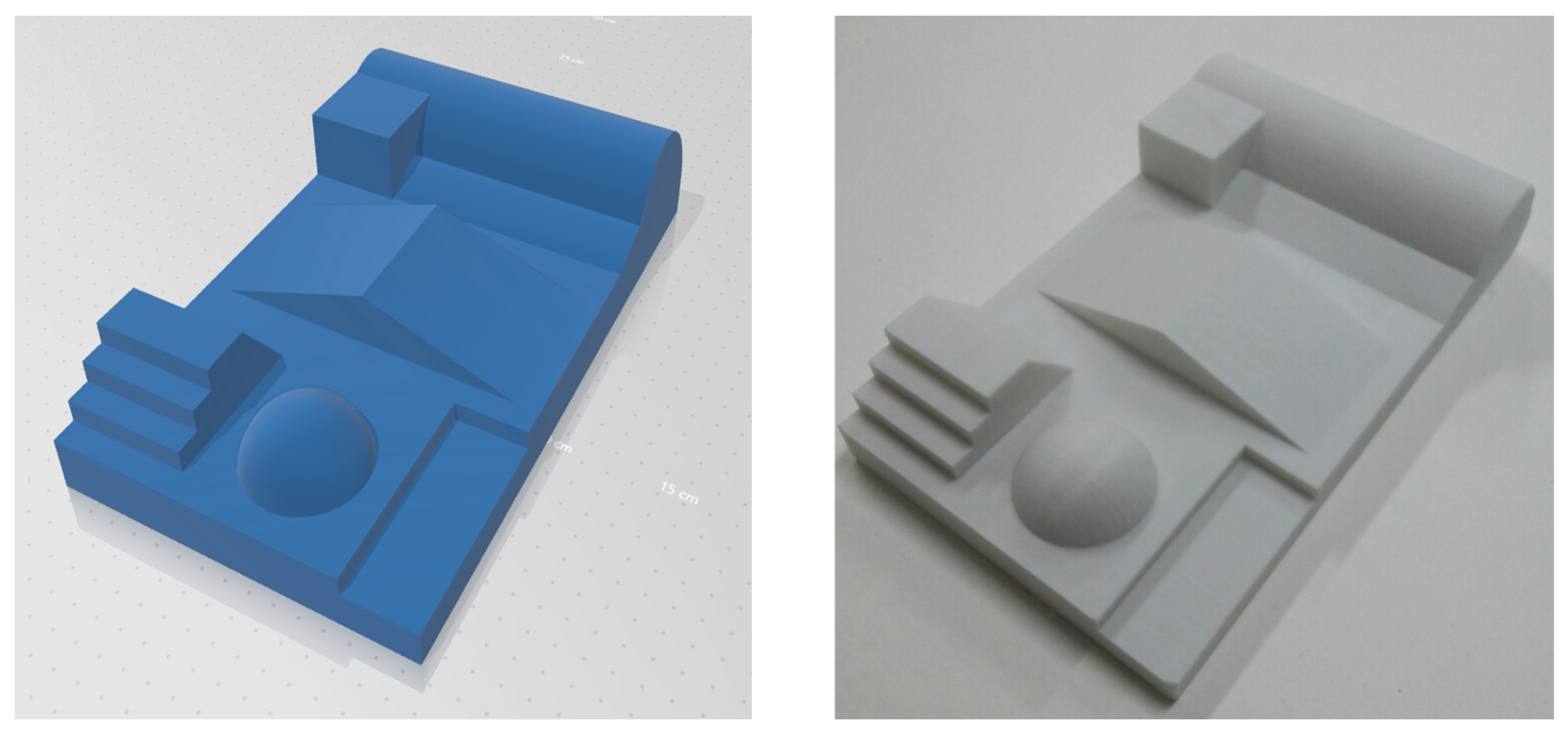
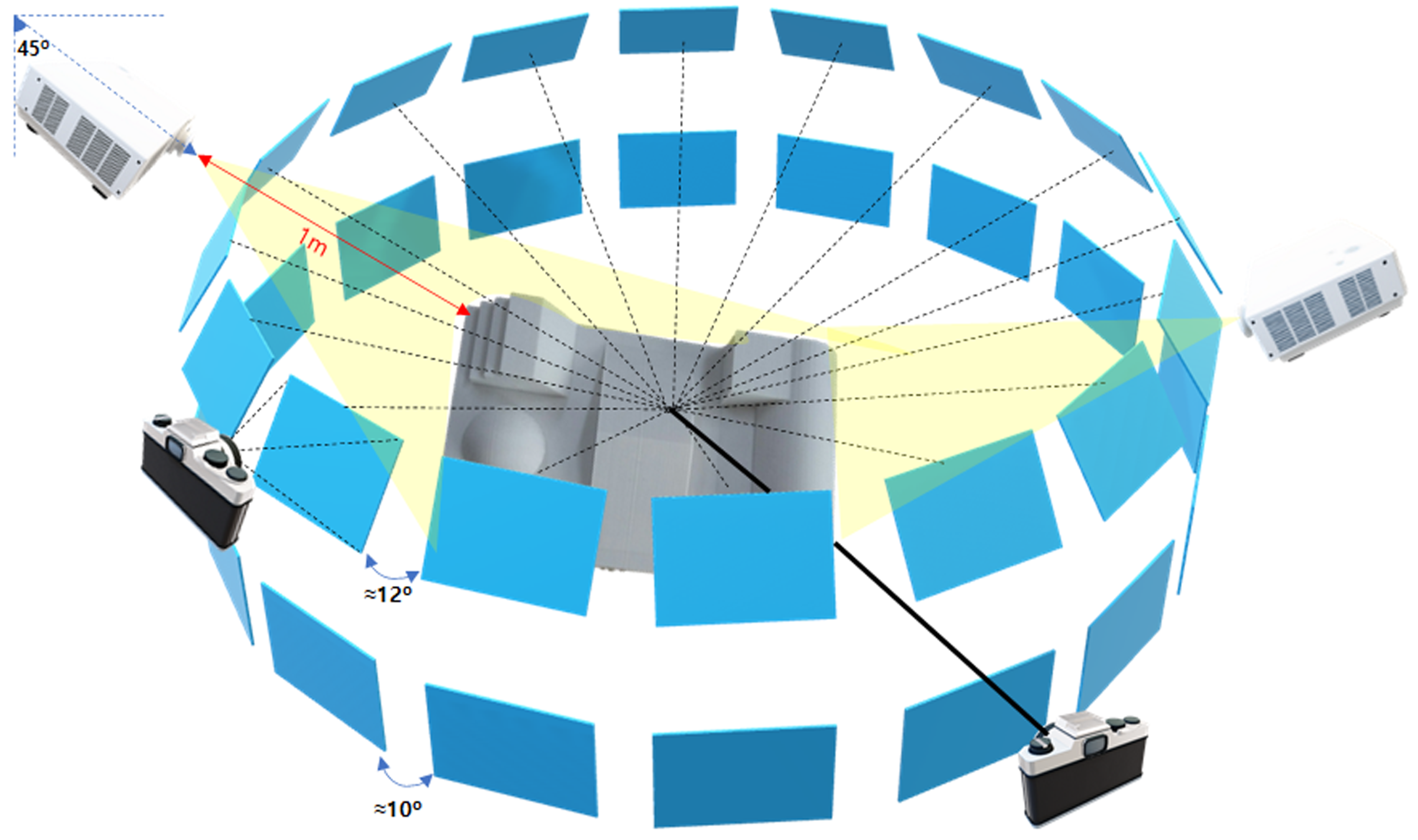
3.2.2. Phase Two: Complex Surface Image Acquisition

In phase two, the best performing pattern from the phase one experiments was used to reconstruct a polygonal 3D model of a test object using all of the feature extraction methods. The test object was produced based on a CAD model using a 3D printer in white color. The dimensions of the printed object were 260 × 150 × 60 mm and contained plane, arc, cylindrical, and spherical shapes, as shown in Figure 3. Owing to its unicolor visual texture, the printed test object is considered to be a very undesirable object for 3D reconstructions by means of SFM-MVS pipelines.

For SFM-MVS pipelines to work, the subject should remain fixed in relation to the capturing device (or vice versa) during the image acquisition process. However, the image acquisition process becomes difficult when the subject has to be artificially enriched with image texture patterns. Two strategies can be adopted to overcome this dilemma: (i) the subject is partially enriched by projecting a pattern using a single projector; or, (ii) the subject is fully enriched with patterns while using multiple projectors, and collect the image data. The first approach is cumbersome, because it requires post-processing steps, including scale and partial scan alignment to merge into a single mesh, which makes it difficult for nonprofessionals. In addition, during the alignment of partial scans, errors can be introduced that affect the quality of the 3D reconstructed model. For these reasons, we selected the second strategy during the image acquisition process, and the camera was only moved in relation to the test object and the video projector that remained fixed during the entire process (Figure 4).

The test object was placed on a static surface throughout the image acquisition process in order to capture the images. Two video projectors were used to completely enrich the test object with the best performing noise pattern (Random Eq) from the phase one experiments that was always projected from the same static position. Both of the projectors were positioned at a distance of 1 m and at an angle of ≈45${}^{\circ }$ to the object, but opposite in the direction. The images were shot at two levels to cover the entire surface of the test object at all possible angles. At the first level, 36 images were captured by rotating the camera manually around the object, while 30 images were captured at the second level. Thus, a total of 66 images were taken, ensuring an overlap of more than 60% between images. In addition, the test object was also captured under daylight conditions without any pattern being applied. The image resolution was set to a maximum of 3648 × 2736 pixels supported by the camera. Following some preliminary tests, the focal length was set to 14 mm with an f-stop of $f/3.5$, shutter speed 1/80 s, and $ISO200$ in order to support the lighting conditions.

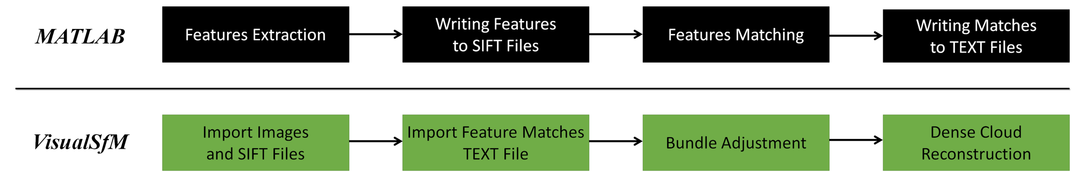
3.3. 3D Reconstruction Using Feature Extraction and Matching Plug-In

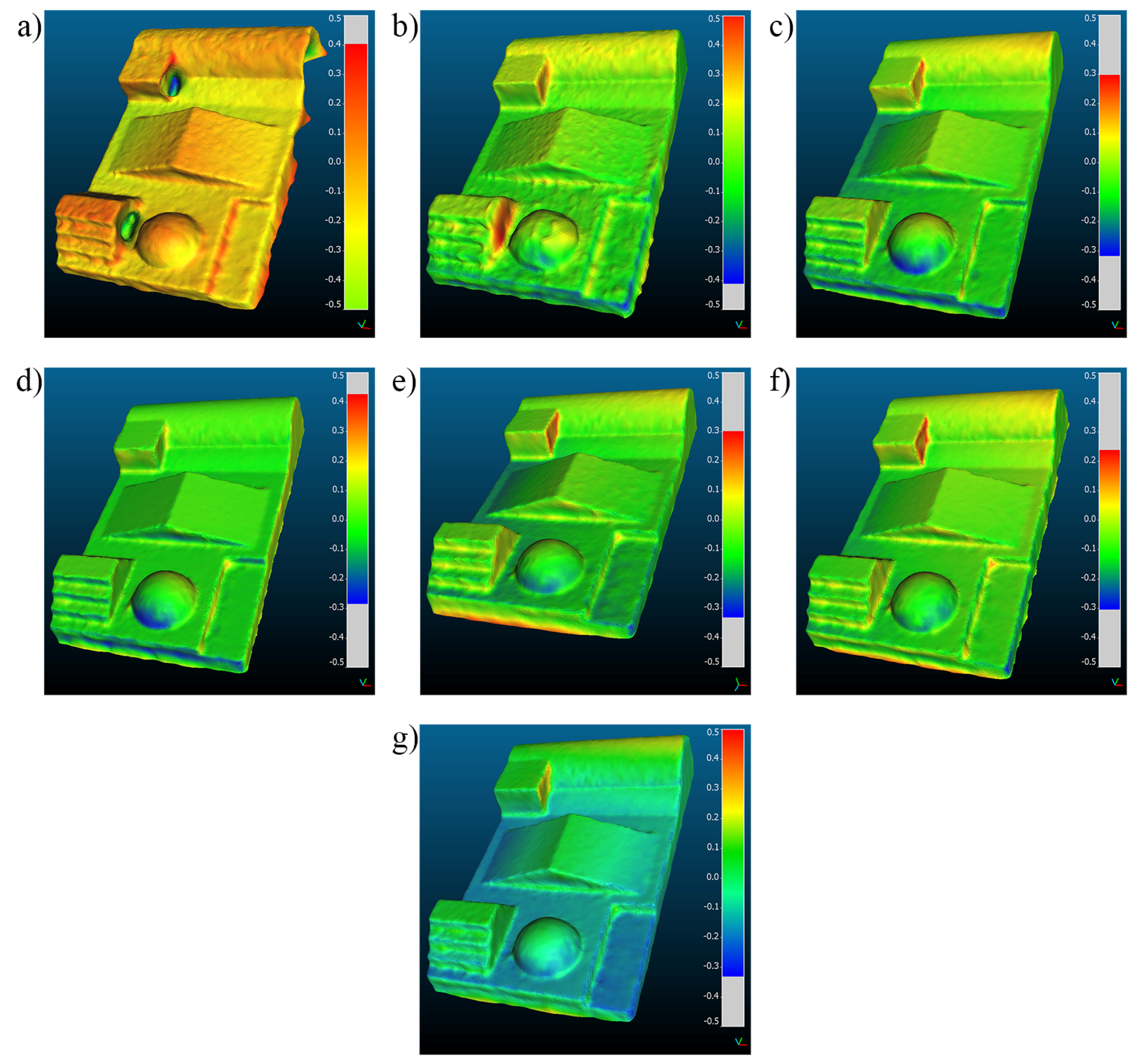
The SFM-MVS-based 3D reconstruction pipeline allows for the generation of 3D models starting from a set of images captured from multiple viewpoints. The SFM-MVS is a sequential pipeline that consists of an initial stage of feature extraction from the images, as discussed in Section 2. The overall performance of the pipeline strongly depends on the quality of the initial feature extraction stage. In computer vision, there are various feature extraction methods for detecting and describing feature points in an image. Therefore, determining which feature extraction method (Section 2.1) delivers the most discriminative power and robustness is significant. However, the SFM-MVS pipelines that are offered by different research groups only include popular methods, such as SIFT or SURF [2]. On the other hand, black-box SFM-MVS-based software such as Agisoft Metashape [44] do not provide any information about the methods. To this end, we developed a MATLAB-based plug-in that includes state-of-the-art algorithms for feature extraction, feature matching, and the generation of SIFT files written in D.G. Lowe’s ASCII format for further proceedings in the pipeline.

The SFM-MVS pipeline is implemented in two segments, as shown in Figure 5. In the first segment, feature detection and description algorithms identify the potential keypoints and localize their position in 2D images while using all methods described in Section 2.1 (except SIFT). Next, the extracted feature points are saved in SIFT files (feature descriptor) while using Lowe’s ASCII format. The header of the SIFT files is composed of the number of detected points and the size of the descriptor. The subsequent lines describe the 2D position and descriptor vector of each feature point identified in the images. For SIFT, SURF, KAZE, and BRISK feature detection methods, their designated feature descriptors are used, while a SURF descriptor is employed for the HARRIS, Shi-Tomasi, and MSER feature detectors. The parameters that are used for feature detection and description for each method are indicated in Appendix A. Subsequently, the extracted feature points are matched between image pairs in the sequence using one of the methods described in Section 2.2. In this work, we used an approximate method of nearest neighbor search to match large sets of image features with threshold-based strategy. The match threshold value was set to 5 for binary (BRISK) and 1 for nonbinary (SURF, KAZE, and SIFT) feature vectors (descriptor) to return only strong matches. Two feature vectors are only matched when the distance between them is less than the threshold value which represents a percent of the distance from the perfect match. The matched feature points are then saved in a text file. The feature matches text file consists of the names of the image pairs, and the total number and indices of the matched features between all of the image pairs. SIFT and feature matching files are written in this way as a VisualSfM prerequisite for the BA process. VisualSfM is an academic program that offers a complete SFM-MVS pipeline [45]. For the SIFT feature extraction method, the entire SFM-MVS pipeline is implemented in VisualSfM for all image sets.

In the second part of the SFM-MVS pipeline, image sets along with the respective SIFT files are imported into VisualSfM for further processing. The text files that comprise the feature matches between image pairs in an image set are also imported. The imported feature matches are filtered while using the RANSAC algorithm to remove the outliers and also to find a transformation function in terms of Homography Matrix. This matrix provides the perspective transform of the second image with respect to the first. The location and orientation of the camera stations and 3D coordinates of tie points on the images in 3D space are estimated, and sparse point clouds are obtained as a result of the bundle adjustment. Finally, using the CMVS-PMVS methods on the sparse cloud of points, dense reconstruction of the model cloud is obtained, which can be transformed into a polygonal 3D model.

4. Results

The dense point clouds that are reconstructed from the image sets collected through real and virtual experiments in phase one (Figure 6) are quantitatively and qualitatively analyzed. The quality of dense point clouds can be evaluated while using different criteria, including the number of vertices (

Table 1. The number of vertices found in the dense point clouds of planar surface reconstruction.

Pattern	HARRIS		Shi-Tomasi		MSER		SIFT		SURF		KAZE		BRISK
	Real	Virtual	Real	Virtual	Real	Virtual	Real	Virtual	Real	Virtual	Real	Virtual	Real	Virtual
Salt Pepper	333,776	374,435	349,877	377,170	349,547	408,694	351,819	388,882	345,854	377,295	336,758	388,948	321,687	370,238
Gaussian	321,254	374,636	324,931	389,168	349,592	389,766	355,264	388,848	332,265	390,024	341,559	377,505	325,654	388,532
Speckle	316,190	389,723	331,225	390,690	311,359	390,762	328,399	408,792	328,996	407,496	384,552	387,681	297,111	388,306
Pi	396,052	388,957	416,462	378,691	372,798	408,658	401,546	408,516	390,739	388,939	386,662	374,973	402,154	379,557
Euler	399,088	389,295	397,218	389,423	406,699	375,686	390,470	390,660	405,226	390,583	381,252	375,611	394,009	389,582
Golden Ratio	400,332	377,244	403,797	389,335	386,266	389,482	392,946	408,541	391,867	390,148	396,991	381,597	395,247	378,049
Random	404,362	376,049	409,327	374,895	393,276	378,269	393,584	384,666	405,537	375,217	388,368	389,247	383,595	378,560
Random Eq	408,148	377,950	401,035	378,761	395,661	392,000	396,536	389,200	387,835	375,170	391,230	376,407	402,779	376,006

) and RMS reprojection error, also known as the standard deviation (

Table 2. The standard deviation calculated for the dense point clouds of planar surface reconstruction while using the best fit method.

Pattern	HARRIS		Shi-Tomasi		MSER		SIFT		SURF		KAZE		BRISK
	Real	Virtual	Real	Virtual	Real	Virtual	Real	Virtual	Real	Virtual	Real	Virtual	Real	Virtual
Salt Pepper	0.007964	0.000727	0.001395	0.002825	0.004711	0.002905	0.002012	0.000851	0.002124	0.005984	0.008351	0.003033	0.012119	0.00451
Gaussian	0.005142	0.004051	0.003201	0.001263	0.003245	0.004886	0.00193	0.000891	0.001664	0.004059	0.002719	0.008868	0.004523	0.004501
Speckle	0.003624	0.006985	0.004261	0.005722	0.005113	0.000764	0.00302	0.000686	0.002735	0.002529	0.002354	0.003657	0.030517	0.007487
Pi	0.001699	0.00202	0.004283	0.002457	0.004052	0.009611	0.000971	0.000909	0.00478	0.0038	0.003925	0.003455	0.001394	0.009267
Euler	0.004596	0.003036	0.006106	0.003678	0.003926	0.002073	0.002374	0.000813	0.005827	0.002245	0.003115	0.002656	0.011435	0.002133
Golden Ratio	0.002782	0.006474	0.002302	0.004619	0.002895	0.004815	0.002319	0.001045	0.001293	0.004292	0.002504	0.003125	0.00494	0.004823
Random	0.004561	0.000614	0.004148	0.007706	0.001869	0.000741	0.001034	0.000819	0.003893	0.006808	0.002048	0.004414	0.002996	0.004258
Random Eq	0.002171	0.000632	0.00251	0.006221	0.001938	0.004773	0.001546	0.000743	0.00339	0.002134	0.002076	0.006545	0.001245	0.000896

). A reprojection error is the distance between a keypoint detected in an image, and a corresponding 3D point reprojected into the same image. This distance is usually calculated while using the best fit method, and it represents surface deviations in the point clouds. The number of vertices provides a quantitative measure and directly reflects the quality of 3D point clouds. Although the reprojection error calculated for a point cloud provides a qualitative measure, it cannot be directly compared with other point clouds. This is due to the varying number of vertices in the point clouds that are input data for the calculation of reprojection errors. Therefore, observing each criterion separately cannot lead to a valid conclusion regarding the quality of 3D reconstruction. The ratio of the number of vertices to the standard deviation is introduced in order to compare the RMS (standard deviation) for each point cloud generated with different feature extraction methods and evaluate the performance of image patterns. The ratio $R_{SD}$ between the number of $Vertices$ and the standard deviation $\left(SD\right)$ expressed in pixels is calculated while using Equation (11).

$$R_{SD}=\frac{Vertices}{SD}$$

(11)

The obtained ratio values are then normalized in Equation (12), where $max{R}_{SD}$ is the highest calculated value of a feature extraction method for each image pattern. Finally, a quality score, Q, for each image pattern, is calculated as the average value of the normalized percentage values of all feature extraction methods (a total of seven methods) through Equation (13).

$$R_{SD\%}=\frac{R_{SD}}{max{R}_{SD}}\times 100$$

(12)

$$Q=\frac{{\sum }_{i=1}^7{R}_{SD\%}\left(i\right)}{7}$$

(13)

The quality score, Q, only provides a relative comparison of the synthetically generated image patterns with employed feature extraction methods from the aspect of 3D reconstruction quality of point clouds. The highest quality score, Q, for an image pattern makes it the best performing among all other image patterns with the assumption that it performed best, on average, with all feature extraction methods.

While using Equations (11)–(13), the 3D reconstruction quality score, Q, for each synthetic image pattern was calculated. Figure 7 provides a graphical representation of the quality score measured for each pattern using the values in Table 1 and Table 2. From the graph, it is evident that the Random Eq pattern obtained the highest quality score in the real experiments. It can be noted that the quality score Q is smaller for the image sets that were collected in the virtual environment, and this behavior can be explained by the lack of noise in virtual images.

In the second phase of the experiments, the true accuracy of the synthetic image pattern is challenged on a texture-less 3D object to find the best feature extraction method. The test object was captured under the projection of the Random Eq pattern, the highest-ranked pattern in Phase One, and polygonal 3D models of the test object were generated while using all of the feature extraction methods. Without any post-processing, the raw 3D polygonal models were evaluated. In order to evaluate the reconstruction quality, the surface deviation comparison between polygonal models and the CAD model (reference model) was carried out while using CloudCompare [46] software. For the evaluation, the polygonal models were registered with the reference model using the ICP algorithm [47], which attempts to minimize the alignment error between the two meshes. As a result of the comparison, the mean distance and standard deviation are calculated. Figure 8 shows the heatmap representation of the calculated distances, where the color-schemes of red, blue, and green represent the positive, negative, and no deviations, respectively, while other deviations are presented in the range of ±0.5 mm. The gray color in the scale bar reflects values that are outside the range. In addition, the Gaussian distribution of the signed distances for all ploygonal 3D models is shown in Figure 9. Furthermore, the 3D reconstruction without the use of any pattern proved to be problematic as the SFM-MVS failed in the spatial alignment of the images due to lack of features.

Table 3. The mean distance and standard deviation calculated for the polygonal models from different feature extraction methods.

Method	Mesh	M. Distance	St. Deviation
	Vertices	[mm]	[mm]
HARRIS	77,875	−0.1134	0.1798
Shi-Tomasi	90,497	0.0183	0.1011
MSER	87,923	−0.0584	0.0758
SIFT	89,334	−0.0099	0.0801
SURF	86,790	−0.0228	0.0822
KAZE	86,198	−0.0092	0.0635
BRISK	85,982	−0.0322	0.0967

indicates the quantitative measures for each polygonal model of the test object while using different feature extraction methods. The Shi-Tomasi method achieved the highest number of vertices in the polygonal models, which can be explained because the algorithm is designed to detect the maximum number of corners in the images. The projection of the image patterns produces many surface features that are well adapted to the Shi-Tomasi algorithm in the feature extraction process. The KAZE method exhibited the lowest mean distance and standard deviation values for the polygonal model when compared with the reference model. This behavior can be explained by the fact that, when blurring the images, the KAZE algorithm preserves the boundaries of the objects, which results in a more accurate matching in the subsequent process; hence, a 3D reconstruction of the better quality.

5. Discussion

Two types of surfaces are used in order to evaluate the behavior of feature detection methods with synthetic noise patterns. In the first phase of experiments, the projection of the pattern is captured on a plane wall in the real environment. Because the surface of the object under observation is plane, the pattern shown in the corresponding image would be similar to that of the projected pattern. In addition, the structure and randomness of the pattern is maintained as well as focus of the projector. Consequently, the 3D reconstruction of the surface is essentially the reconstruction of the pattern itself. These factors prove the ability of this method to examine the efficiency of image patterns and find their accuracy.

In phase one experiments, the point clouds of virtual planar surfaces generally resulted in more vertices than the real planar surfaces and the quality graph also tends to be more consistent. This can be explained by the fact that in the case of real experiments, the pixels of the pattern image can lose or change their intensity when projected on the wall. Additionally, the surface color, lighting conditions, and limitations of the projection system (such as color aberration) can affect the projected image. However, these factors are not involved in the case of virtual experiments. Therefore, synthetic image patterns can behave differently in real and virtual environments. As shown in Figure 7, the Random Eq pattern, the highest ranked pattern in real conditions, achieved a quality score of about 20% higher than the worst (Salt&Pepper) pattern, while it scored lower (5%) than the same pattern in the simulated environment.

The polygonal models that are generated in the second phase of the experiments are analyzed in order to evaluate the performance of the feature extraction methods. Because the experiments were performed under real conditions, only the highest ranked pattern from the phase one real environment is used during the image acquisition process. All of the feature detection methods were able to recreate 3D polygonal models of the test object with varying accuracy. Because the Gaussian distribution of the measured distances (Figure 9a) is widespread with a mean distance of $-0.113\mathrm{mm}$, the Harris corner detector exhibited maximum deviation $\left(0.179\mathrm{mm}\right)$. While the efficiency gain for other feature extraction methods (Shi-Tomasi 43%, MSER 58%, SIFT 55%, SURF 54%, KAZE 64%, and BRISK 48%) is observed as compared to the Harris detector in terms of standard deviation. Because 3D printing technology (Sindoh 2X Series) was used to create the test object, dimensional inaccuracies can occur during the printing process. To determine this error, the printed object was measured from 12 different places while using a digital vernier caliper and the difference was found from the corresponding locations on the CAD model. Subsequently, descriptive statistics, including mean $\left(0.055\mathrm{mm}\right)$, standard deviation $\left(0.12\mathrm{mm}\right)$, median $\left(0.13\mathrm{mm}\right)$, min $(-0.3\mathrm{mm})$, max $\left(0.3\mathrm{mm}\right)$, and RMS $\left(0.202\mathrm{mm}\right)$ of those differences were calculated. Although the dimensional inaccuracies (very small) are present in the printed object, they remain constant for all of the evaluated polygonal 3D models.

6. Conclusions

In this paper, we evaluated the performance of feature extraction methods with synthetic noise patterns on texture-less surfaces. Seven state-of-the-art feature detector algorithms were included for feature extraction and then tested on a planar and a challenging object. Experiments were conducted in two phases, one of which culminated in the best performing pattern used to reconstruct a texture-less object in the second phase to find the best feature extraction method. The best performing pattern was one with the highest quality score average that was determined by considering all feature detector algorithms. We discovered that the Random Eq. pattern achieved higher quality score (63%) as compared to the other noise pattern, followed by the Gaussian (61%) and Euler (56%) noise patterns, respectively. The characteristics of the patterns involved intensity histograms and the Random Eq pattern has a uniform distribution of the intensity histogram.

Due to its performance and the application of the Random Eq pattern, polygonal models of the test object were generated for each feature extraction method. When compared to the CAD model, the polygonal model that was generated with the KAZE algorithm showed minimal deviations. Furthermore, the high number of mesh vertices does not ensure higher efficiency, as the KAZE detector produced 86K (with 64% gain) of mesh vertices, while the Shi-Tomasi detector obtained 90K (with 43% gain). Depending on the application, where the surface texture is important, it is vital to choose the right feature detector for high quality 3D reconstruction. For instance, high quality is desirable in preserving cultural heritage artifacts or creating replicas. The choice of a feature detection method and a synthetic image pattern can substantially increase the accuracy of the reconstructed polygonal 3D model.

While 3D reconstruction of texture-less objects using synthetic image patterns is a viable solution where no other digitization approaches are possible or applicable, it is rather limited to indoor conditions. Although the use of multiple projectors eliminates the need of post-processing, the image acquisition stage is still time consuming and needs a very experienced camera operator. A compact system, such as multi-camera rig system with multiple projectors, can overcome some of the limitations and reduce the duration of image acquisition. Further research will focus on achieving a greater degree of automation in image acquisition for texture-less 3D surface reconstruction while using SFM-MVS pipelines.

References

1. Aicardi, I.; Chiabrando, F.; Lingua, A.M.; Noardo, F. Recent trends in cultural heritage 3D survey: The photogrammetric computer vision approach. J. Cult. Herit. 2018, 32, 257–266. [Google Scholar] [CrossRef]
2. Bianco, S.; Ciocca, G.; Marelli, D. Evaluating the Performance of Structure from Motion Pipelines. J. Imaging 2018, 4, 98. [Google Scholar] [CrossRef] [Green Version]
3. Chang, Y.C.; Detchev, I.; Habib, A. A photogrammetric system for 3D reconstruction of a scoliotic torso. In Proceedings of the ASPRS 2009 Annual Conference, Baltimore, MD, USA, 9–13 March 2009; p. 12. [Google Scholar]
4. Poux, F.; Valembois, Q.; Mattes, C.; Kobbelt, L.; Billen, R. Initial User-Centered Design of a Virtual Reality Heritage System: Applications for Digital Tourism. Remote Sens. 2020, 12, 2583. [Google Scholar] [CrossRef]
5. Bruno, F.; Bruno, S.; De Sensi, G.; Luchi, M.L.; Mancuso, S.; Muzzupappa, M. From 3D reconstruction to virtual reality: A complete methodology for digital archaeological exhibition. J. Cult. Herit. 2010, 11, 42–49. [Google Scholar] [CrossRef]
6. Kim, J.M.; Shin, D.K.; Ahn, E.Y. Image-Based Modeling for Virtual Museum. In Multimedia, Computer Graphics and Broadcasting; Kim, T.H., Adeli, H., Grosky, W.I., Pissinou, N., Shih, T.K., Rothwell, E.J., Kang, B.H., Shin, S.J., Eds.; Springer: Berlin/Heidelberg, Germany, 2011; Volume 262, pp. 108–119. [Google Scholar]
7. Zancajo-Blazquez, S.; Gonzalez-Aguilera, D.; Gonzalez-Jorge, H.; Hernandez-Lopez, D. An Automatic Image-Based Modelling Method Applied to Forensic Infography. PLoS ONE 2015, 10, e0118719. [Google Scholar] [CrossRef]
8. Laviada, J.; Arboleya-Arboleya, A.; Álvarez, Y.; González-Valdés, B.; Las-Heras, F. Multiview three- dimensional reconstruction by millimetre-wave portable camera. Sci. Rep. 2017, 7, 6479. [Google Scholar] [CrossRef]
9. Hammond, J.E.; Vernon, C.A.; Okeson, T.J.; Barrett, B.J.; Arce, S.; Newell, V.; Janson, J.; Franke, K.W.; Hedengren, J.D. Survey of 8 UAV Set-Covering Algorithms for Terrain Photogrammetry. Remote Sens. 2020, 12, 2285. [Google Scholar] [CrossRef]
10. Forsmoo, J.; Anderson, K.; Macleod, C.J.A.; Wilkinson, M.E.; DeBell, L.; Brazier, R.E. Structure from motion photogrammetry in ecology: Does the choice of software matter? Ecol. Evol. 2019, 9, 12964–12979. [Google Scholar] [CrossRef]
11. Iglhaut, J.; Cabo, C.; Puliti, S.; Piermattei, L.; O’Connor, J.; Rosette, J. Structure from Motion Photogrammetry in Forestry: A Review. Curr. For. Rep. 2019, 5, 155–168. [Google Scholar] [CrossRef] [Green Version]
12. Hamacher, A.; Kim, S.J.; Cho, S.T.; Pardeshi, S.; Lee, S.H.; Eun, S.J.; Whangbo, T.K. Application of Virtual, Augmented, and Mixed Reality to Urology. Int. Neurourol. J. 2016, 20, 172–181. [Google Scholar] [CrossRef]
13. Perez, E.; Merchan, P.; Merchan, M.J.; Salamanca, S. Virtual Reality to Foster Social Integration by Allowing Wheelchair Users to Tour Complex Archaeological Sites Realistically. Remote Sens. 2020, 12, 419. [Google Scholar] [CrossRef] [Green Version]
14. Buyukdemircioglu, M.; Kocaman, S. Reconstruction and Efficient Visualization of Heterogeneous 3D City Models. Remote Sens. 2020, 12, 2128. [Google Scholar] [CrossRef]
15. Bassier, M.; Vincke, S.; De Lima Hernandez, R.; Vergauwen, M. An Overview of Innovative Heritage Deliverables Based on Remote Sensing Techniques. Remote Sens. 2018, 10, 1607. [Google Scholar] [CrossRef] [Green Version]
16. Lee, J.; Hafeez, J.; Kim, K.; Lee, S.; Kwon, S. A Novel Real-Time Match-Moving Method with HoloLens. Appl. Sci. 2019, 9, 2889. [Google Scholar] [CrossRef] [Green Version]
17. Ozyesil, O.; Voroninski, V.; Basri, R.; Singer, A. A Survey of Structure from Motion. arXiv 2017, arXiv:1701.08493. [Google Scholar]
18. Engler, O.; Randle, V. Introduction to Texture Analysis: Macrotexture, Microtexture, and Orientation Mapping, 2nd ed.; Google-Books-ID: MpLq_0Bkn6cC; CRC Press: Boca Raton, FL, USA, 2009. [Google Scholar]
19. Ahmadabadian, A.H.; Yazdan, R.; Karami, A.; Moradi, M.; Ghorbani, F. Clustering and selecting vantage images in a low-cost system for 3D reconstruction of texture-less objects. Measurement 2017, 99, 185–191. [Google Scholar] [CrossRef]
20. Hosseininaveh Ahmadabadian, A.; Karami, A.; Yazdan, R. An automatic 3D reconstruction system for texture-less objects. Robot. Auton. Syst. 2019, 117, 29–39. [Google Scholar] [CrossRef]
21. Koutsoudis, A.; Ioannakis, G.; Vidmar, B.; Arnaoutoglou, F.; Chamzas, C. Using noise function-based patterns to enhance photogrammetric 3D reconstruction performance of featureless surfaces. J. Cult. Herit. 2015, 16, 664–670. [Google Scholar] [CrossRef]
22. Santosi, Z.; Budak, I.; Stojakovic, V.; Sokac, M.; Vukelic, D. Evaluation of synthetically generated patterns for image-based 3D reconstruction of texture-less objects. Measurement 2019, 147, 106883. [Google Scholar] [CrossRef]
23. Hafeez, J.; Kwon, S.C.; Lee, S.H.; Hamacher, A. 3D surface reconstruction of smooth and textureless objects. In Proceedings of the International Conference on Emerging Trends Innovation in ICT (ICEI), Pune, India, 3–5 February 2017; pp. 145–149. [Google Scholar]
24. Hafeez, J.; Lee, S.; Kwon, S.; Hamacher, A. Image Based 3D Reconstruction of Texture-less Objects for VR Contents. Int. J. Adv. Smart Converg. 2017, 6, 9–17. [Google Scholar] [CrossRef] [Green Version]
25. Hafeez, J.; Jeon, H.J.; Hamacher, A.; Kwon, S.C.; Lee, S.H. The effect of patterns on image-based modelling of texture-less objects. Metrol. Meas. Syst. 2018, 25, 755–767. [Google Scholar]
26. Harris, C.; Stephens, M. A combined corner and edge detector. In Proceedings of the Fourth Alvey Vision Conference, Manchester, UK, 31 August–2 September 1988; pp. 147–151. [Google Scholar]
27. Shi, J.; Tomasi. Good features to track. In Proceedings of the IEEE Conference on Computer Vision and Pattern Recognition, Seattle, WA, USA, 21–23 June 1994; pp. 593–600. [Google Scholar]
28. Leutenegger, S.; Chli, M.; Siegwart, R.Y. BRISK: Binary Robust invariant scalable keypoints. In Proceedings of the International Conference on Computer Vision, Barcelona, Spain, 6–13 November 2011; pp. 2548–2555. [Google Scholar]
29. Lowe, D.G. Distinctive Image Features from Scale-Invariant Keypoints. Int. J. Comput. Vis. 2004, 60, 91–110. [Google Scholar] [CrossRef]
30. Bay, H.; Tuytelaars, T.; Van Gool, L. SURF: Speeded Up Robust Features. In Lecture Notes in Computer Science, Proceedings of the Computer Vision—ECCV, Graz, Austria, 7–13 May 2006; Leonardis, A., Bischof, H., Pinz, A., Eds.; Springer: Berlin/Heidelberg, Germany, 2006; pp. 404–417. [Google Scholar]
31. Alcantarilla, P.F.; Bartoli, A.; Davison, A.J. KAZE Features. In Lecture Notes in Computer Science, Proceedings of the Computer Vision—ECCV, Florence, Italy, 7–13 October 2012; Fitzgibbon, A., Lazebnik, S., Perona, P., Sato, Y., Schmid, C., Eds.; Springer: Berlin/Heidelberg, Germany, 2012; pp. 214–227. [Google Scholar]
32. Matas, J.; Chum, O.; Urban, M.; Pajdla, T. Robust wide-baseline stereo from maximally stable extremal regions. Image Vis. Comput. 2004, 22, 761–767. [Google Scholar] [CrossRef]
33. MATLAB—The MathWorks Inc. Available online: www.mathworks.com (accessed on 10 August 2020).
34. Tomasi, C.; Kanade, T. Detection and Tracking of Point Features; Technical Report; Carnegie Mellon University: Pittsburgh, PA, USA, 1991. [Google Scholar]
35. Wu, C. SiftGPU: A GPU Implementation of Scale Invariant Feature Transform (SIFT). Available online: http://cs.unc.edu/ccwu/siftgpu (accessed on 10 August 2020).
36. Mikolajczyk, K.; Schmid, C. A performance evaluation of local descriptors. IEEE Trans. Pattern Anal. Mach. Intell. 2005, 27, 1615–1630. [Google Scholar] [CrossRef] [Green Version]
37. Fischler, M.A.; Bolles, R.C. Random sample consensus: A paradigm for model fitting with applications to image analysis and automated cartography. Commun. ACM 1981, 24, 381–395. [Google Scholar] [CrossRef]
38. Chum, O.; Matas, J. Matching with PROSAC—Progressive sample consensus. In Proceedings of the IEEE Computer Society Conference on Computer Vision and Pattern Recognition (CVPR’05), San Diego, CA, USA, 20–25 June 2005; Volume 1, pp. 220–226. [Google Scholar]
39. Triggs, B.; McLauchlan, P.F.; Hartley, R.I.; Fitzgibbon, A.W. Bundle Adjustment—A Modern Synthesis. In Lecture Notes in Computer Science, Proceedings of the Vision Algorithms: Theory and Practice, Corfu, Greece, 21–22 September 1999; Triggs, B., Zisserman, A., Szeliski, R., Eds.; Springer: Berlin/Heidelberg, Germany, 2000; pp. 298–372. [Google Scholar]
40. Furukawa, Y.; Curless, B.; Seitz, S.M.; Szeliski, R. Towards Internet-scale multi-view stereo. In Proceedings of the IEEE Computer Society Conference on Computer Vision and Pattern Recognition, San Francisco, CA, USA, 13–18 June 2010; pp. 1434–1441. [Google Scholar]
41. Furukawa, Y.; Ponce, J. Accurate, Dense, and Robust Multiview Stereopsis. IEEE Trans. Pattern Anal. Mach. Intell. 2010, 32, 1362–1376. [Google Scholar] [CrossRef]
42. Kazhdan, M.; Funkhouser, T.; Rusinkiewicz, S. Rotation Invariant Spherical Harmonic Representation of 3D Shape Descriptors. In Proceedings of the Eurographics Symposiumon Geometry Processing, Aachen, Germany, 23–25 June 2003; p. 9. [Google Scholar]
43. Blender Online Community. blender.org—Home of the Blender Project—Free and Open 3D Creation Software. Available online: www.blender.org (accessed on 10 August 2020).
44. Agisoft Metashape. Agisoft LLC: St. Petersburg, Russia. Available online: www.https://www.agisoft.com (accessed on 10 August 2020).
45. Wu, C. Towards Linear-Time Incremental Structure from Motion. In Proceedings of the 2013 International Conference on 3D Vision, 3DV’13, Seattle, WA, USA, 29 June–1 July 2013; IEEE Computer Society: Washington, DC, USA, 2013; pp. 127–134. [Google Scholar]
46. CloudCompare—Open Source Project. Available online: www.cloudcompare.org (accessed on 10 August 2020).
47. Besl, P.J.; McKay, H.D. A method for registration of 3-D shapes. IEEE Trans. Pattern Anal. Mach. Intell. 1992, 14, 239–256. [Google Scholar] [CrossRef]
Figure 1. Partial bitmap representation of the synthetic noise patterns and their intensity histograms.
Remotesensing 12 03886 g001
Figure 2. Experimental setup for image acquisition in (left) real (right) virtual environments.
Remotesensing 12 03886 g002
Figure 3. The test object used for the evaluation of feature extraction methods.
Remotesensing 12 03886 g003
Figure 4. Image acquisition scheme for the test object using two projectors and one camera.
Remotesensing 12 03886 g004
Figure 5. Workflow diagram of three-dimensional (3D) reconstruction using structure-from-motion coupled with multi-view stereo (SFM-MVS) pipeline.
Remotesensing 12 03886 g005
Figure 6. Dense point clouds generated by image data collected in (left) real and (right) virtual environments.
Remotesensing 12 03886 g006
Figure 7. The quality score graph of the point clouds from phase one real and virtual experiments.
Remotesensing 12 03886 g007
Figure 8. The heatmap representation of the test object for (a) HARRIS, (b) Shi-Tomasi, (c) MSER, (d) SIFT, (e) SURF, (f) KAZE, and (g) BRISK feature extraction methods. Grey color on the scle-bar represents values out of range.
Remotesensing 12 03886 g008
Figure 9. The signed distances of the test object for (a) HARRIS, (b) Shi-Tomasi, (c) MSER, (d) SIFT, (e) SURF, (f) KAZE, and (g) BRISK feature extraction methods.
Remotesensing 12 03886 g009