A Simple Spatio–Temporal Data Fusion Method Based on Linear Regression Coefficient Compensation


1
School of Transportation Science and Engineering, Beihang University, Beijing 100191, China
2
Hydrology and Quantitative Water Management Group, Department of Environmental Sciences, Wageningen University, 6700 AA Wageningen, The Netherlands
3
Deltares, 2629 HV Delft, The Netherlands
*
Author to whom correspondence should be addressed.
Remote Sens. 2020, 12(23), 3900; https://0-doi-org.brum.beds.ac.uk/10.3390/rs12233900
Submission received: 24 September 2020
/
Revised: 23 November 2020
/
Accepted: 26 November 2020
/
Published: 28 November 2020
(This article belongs to the Special Issue Google Earth Engine: Cloud-Based Platform for Earth Observation Data and Analysis)
Abstract
:High spatio–temporal resolution remote sensing images are of great significance in the dynamic monitoring of the Earth’s surface. However, due to cloud contamination and the hardware limitations of sensors, it is difficult to obtain image sequences with both high spatial and temporal resolution. Combining coarse resolution images, such as the moderate resolution imaging spectroradiometer (MODIS), with fine spatial resolution images, such as Landsat or Sentinel-2, has become a popular means to solve this problem. In this paper, we propose a simple and efficient enhanced linear regression spatio–temporal fusion method (ELRFM), which uses fine spatial resolution images acquired at two reference dates to establish a linear regression model for each pixel and each band between the image reflectance and the acquisition date. The obtained regression coefficients are used to help allocate the residual error between the real coarse resolution image and the simulated coarse resolution image upscaled by the high spatial resolution result of the linear prediction. The developed method consists of four steps: (1) linear regression (LR), (2) residual calculation, (3) distribution of the residual and (4) singular value correction. The proposed method was tested in different areas and using different sensors. The results show that, compared to the spatial and temporal adaptive reflectance fusion model (STARFM) and the flexible spatio–temporal data fusion (FSDAF) method, the ELRFM performs better in capturing small feature changes at the fine image scale and has high prediction accuracy. For example, in the red band, the proposed method has the lowest root mean square error (RMSE) (ELRFM: 0.0123 vs. STARFM: 0.0217 vs. FSDAF: 0.0224 vs. LR: 0.0221). Furthermore, the lightweight algorithm design and calculations based on the Google Earth Engine make the proposed method computationally less expensive than the STARFM and FSDAF.
1. Introduction
With the development of Earth observation technology over the last few decades, a large amount of time series of satellite images have been accumulated, and the number of freely available satellite images is growing at fast pace. For example, Landsat data became available at no cost in 2008 [1]. In 2015 and 2017, Sentinel-2A and Sentinel-2B satellites were launched with the data freely available to everyone without any restrictions [2]. In recent years, the Google Earth Engine (GEE), a planetary-scale platform with the capability to process massive satellite images, facilitated the application of satellite image time series to large-scale land and water monitoring [3,4,5,6,7,8]. Therefore, time series-based research has developed considerably in the last decade [9,10,11,12].
However, currently available satellite sensors still cannot meet the demands of the rapid changes monitoring in time series studies [13,14,15], such as high-frequency mapping of the landslides and floods [16], monitoring the phenological changes of crops [17,18], monitoring coal fires [19], and other emergency events. Time series satellite images with the high spatial and temporal resolution are required for these studies, which are difficult to obtain. Because the trade-off between swath width and pixel resolution, it is difficult for existing satellites to acquire images with both high temporal and spatial resolution [20,21]. Although companies, such as Planet, have announced that they can capture high spatial resolution images of the Earth once a day, these images are mainly commercially available, restricting their use only to a limited number of applications. On the other hand, in some regions, particularly in cloudy tropical regions, the availability of cloud-free optical remote sensing data is greatly reduced due to cloud contamination [22].
The spatio–temporal fusion of multi-source satellite images is an effective method to solve the above problems [23,24,25]. It mixes fine spatial resolution data (e.g., Landsat or Sentinel-2) with coarse spatial resolution data, such as the moderate resolution imaging spectroradiometer (MODIS) or Sentinel-3, to improve the temporal resolution of the fine spatial resolution data. Different from other image synthesis techniques, including the intermediate value synthesis method and time series interpolation method, the spatio–temporal fusion method exploits the value of images with a low spatial but high temporal resolution to improve the temporal resolution of the time series. The spatio–temporal fusion method is of great significance for the research applications focusing on the monitoring of the dynamics of Earth’s land-use changes.
Various spatio–temporal fusion algorithms have been developed in the past ten years, including fusion methods for surface reflectance [26,27], specific parameters or indices, such as the normalized difference vegetation index (NDVI) [28], leaf area index (LAI) [29] and land surface temperature (LST) [30]. Spatio–temporal fusion algorithms can be divided into machine learning-based methods [31], unmixing-based methods [32], and the spatial and temporal adaptive reflectance fusion model (STARFM) [33] or its improved methods [32,34]. The methods based on machine learning learn the relationship between the coarse–fine image pairs to guide the predictions of fine images from coarse images [35]. This method predicts reflectance changes in a unified framework, and it is difficult to distinguish the land cover changes [27]. The unmixing-based methods typically require a land-use/land-cover (LULC) image with fine spatial resolution as assistance and assume that (1) no LULC change occurs during the study period, and (2) the proportions of land cover types are constant for low spatial resolution images on different dates. The STARFM, although developed more than ten years ago, it and its improved algorithms are widely used in current research. They are continuously being adapted and improved for different situations, such as the enhanced STARFM (ESTARFM), which increases STARFM’s accuracy in heterogeneous areas [36]. The STARFM and STARFM-derived methods assume no LULC change occurs between the reference and prediction time [33,37], and are proposed base on the two hypotheses: (1) the same type of ground objects in a neighborhood have the same reflectance, and (2) the types of ground objects in the front- and back-phase images are invariable. Therefore, they can predict reflectance changes, such as changes in vegetation phenology, as these changes are closely related to similar pixels selected from the reference image. The flexible spatio–temporal data fusion (FSDAF) method [26] is based on spectral unmixing and thin-plate spline interpolation, which can maintain more spatial details compared to STARFM. However, these existing methods are not effective in predicting sudden spectral changes, as the changes cannot be predicted from similar pixels at the reference time. These changes include flooding, seasonal water level fluctuations, and other land cover transitions. Moreover, most of the existing fusion algorithms are relatively complex in design and low in calculation efficiency that does not scale that well on GEE, which hinders their applications [38]. In 2018, a fusion algorithm called Fit-FC [39] was developed based on linear regression (LR) for nearly daily Sentinel-2 image creation and presented satisfactory accuracy. It includes three steps of regression model fitting, spatial filtering, and residual compensation. Several studies showed that, compared with the STARFM and ESTARFM methods, the linear interpolation model (LIM) can produce higher prediction accuracy sometimes [40].
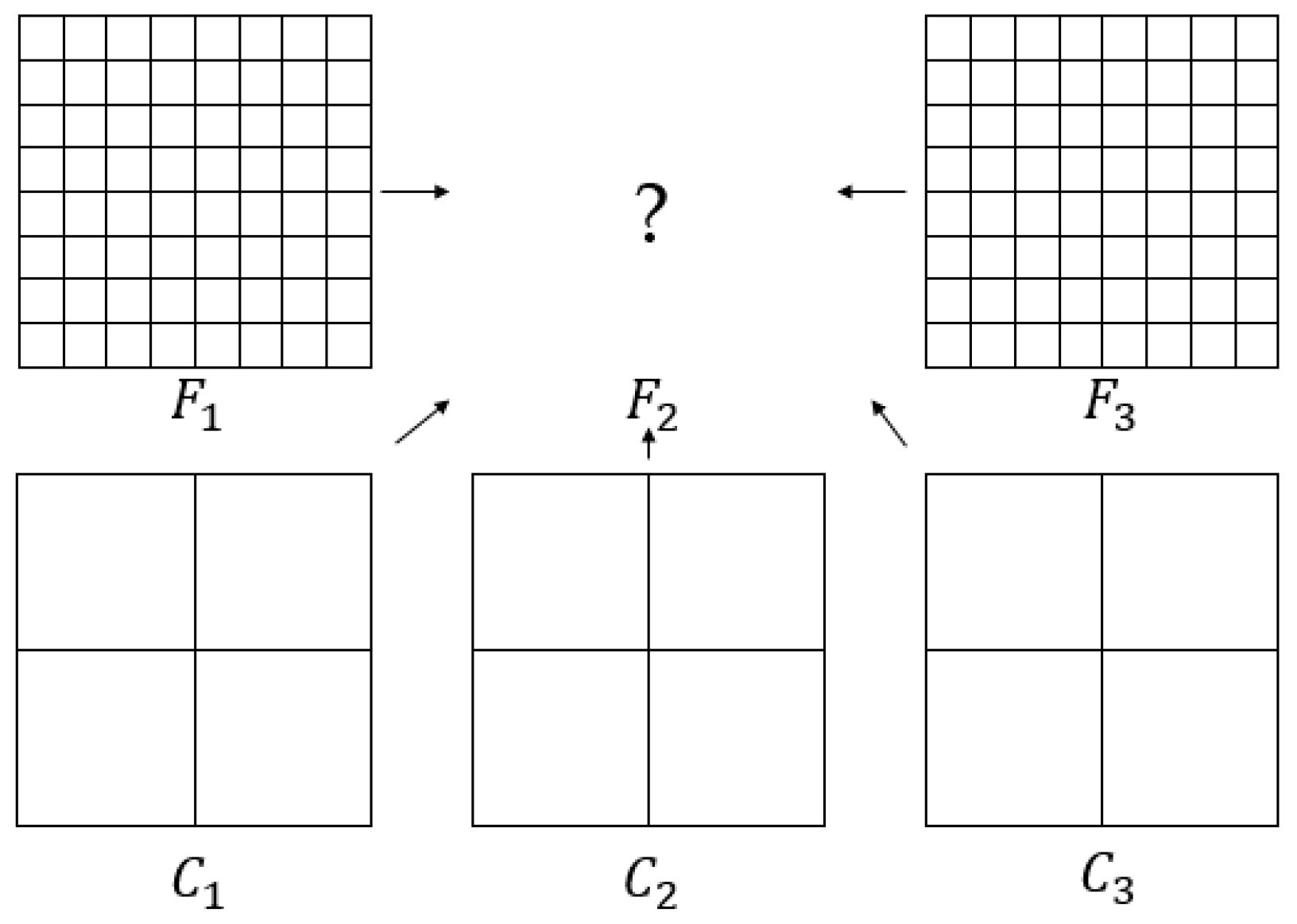
Here, we propose a new simple enhanced linear regression spatio–temporal fusion method (ELRFM). This method uses two pairs of fine–coarse (i.e., Landsat-MODIS) spatial resolution images acquired at the reference dates and one coarse MODIS image acquired at a prediction date to generate a fine resolution image at the prediction date (Figure 1). The developed method builds a linear regression model, using two fine resolution images acquired at the reference dates, between the image reflectance and the acquisition date for each pixel and each band. The regression coefficients are used to assign residuals which are calculated from the coarse images to compensate for the result of the first linear prediction to further improve the prediction accuracy. The proposed method can be used to predict fine spatial resolution images in heterogeneous areas with abrupt LULC changes and has good adaptability on different remote sensing data sources (e.g., Sentinel-2 and Sentinel-3).
2. Materials and Methods
2.1. Data
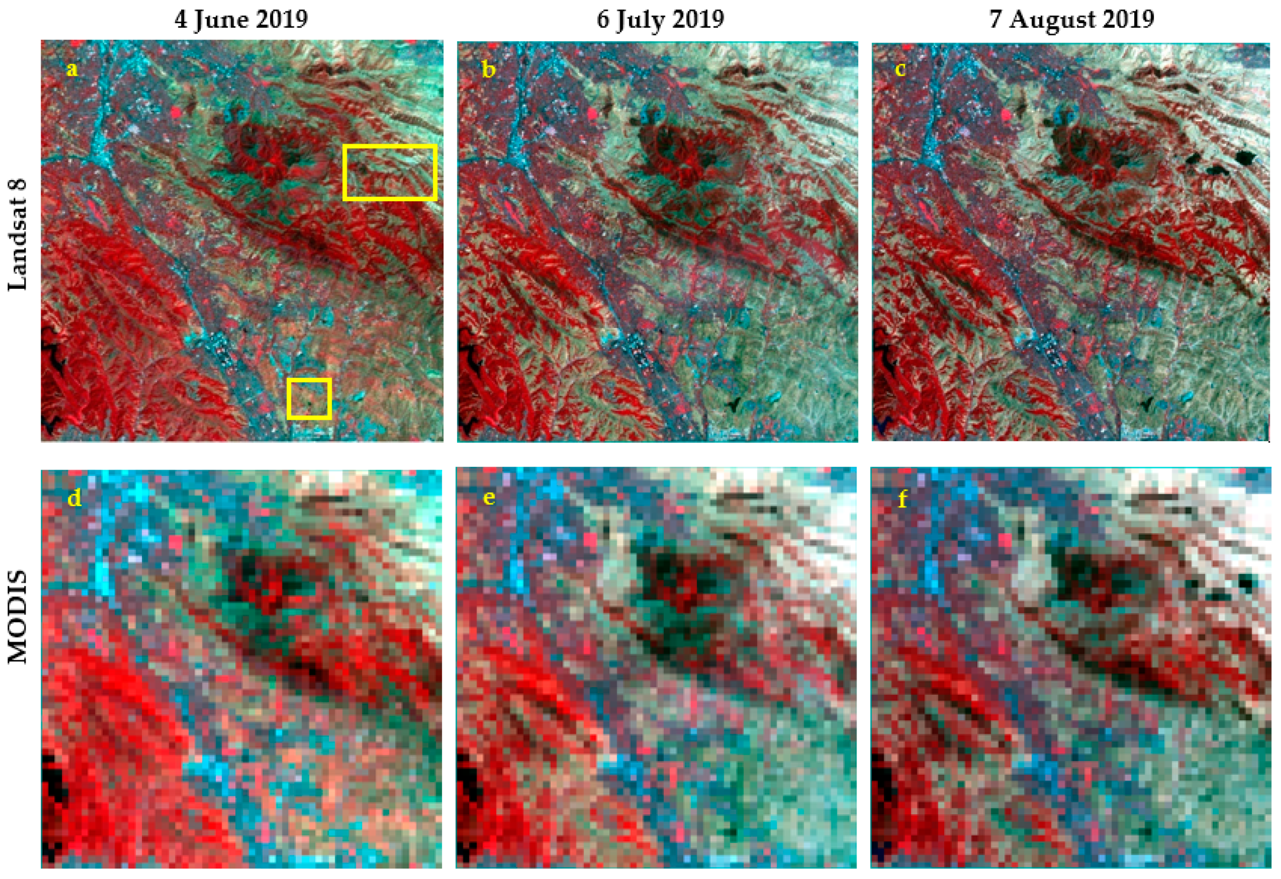
Landsat 8 top-of-atmosphere (TOA) images archived in GEE platform with a 30 m spatial resolution acquired on 4 June (), 6 July (), and 7 August () 2019 from operational land imager (OLI) sensor, with Worldwide Reference System (WRS)-2 path/row of 44/34 were used. The study area is a subset of one TOA scene covering an area of 28.8 km × 28.8 km (960 × 960 pixels) (Figure 2). The LULC of the areas marked by yellow rectangles in Figure 2 changes during the study period, which can help to evaluate the performance of the ELRFM. The coarse spatial resolution images used are the simulated MODIS aggregated from Landsat.
2.2. Methods
2.2.1. Data Pre-Processing and Environment
The strategy of conducting tests on simulated images was adopted, that is, the high spatial resolution images used the original Landsat 8 images, while the coarse spatial resolution images used the simulated MODIS images, which were aggregated from Landsat. This strategy is adopted by many spatio–temporal fusion studies [26,41,42] to avoid the interference caused by the radiometric or geometric inconsistencies between two sensors. The application of the proposed method to real scenarios and the evaluation of the effects of the above are beyond the scope of this research, but they will be tested and discussed in our future research.
The simulated MODIS images were obtained by upscaling the Landsat images to a spatial resolution of 480 m. The Landsat 8 images acquired on 4 June and 7 August 2019 and the MODIS image simulated from the Landsat 8 image acquired on 6 July 2019 were used as the input for the fusion algorithm. The task is to predict the high spatial resolution Landsat-like image on 6 July 2019. The original Landsat 8 image acquired on 6 July 2019 is later adopted for evaluation (i.e., not used as the algorithm input).
The proposed method runs on the GEE platform and is written with JavaScript.
2.2.2. Enhanced Linear Regression Spatio-Temporal Fusion Method
The ELRFM is based on two assumptions: (1) if there is no change in the reflectance of the ground object between the two Landsat reference images, the reflectance of the object in the predicted image does not change either (that is, the prediction error mainly comes from the areas where the reflectance changes greatly between the two reference images); and (2) the reflectance relationship between the Landsat image and the MODIS image at different times is consistent.
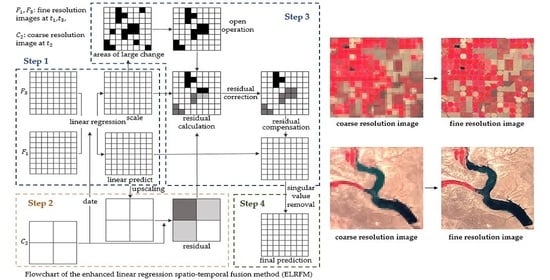
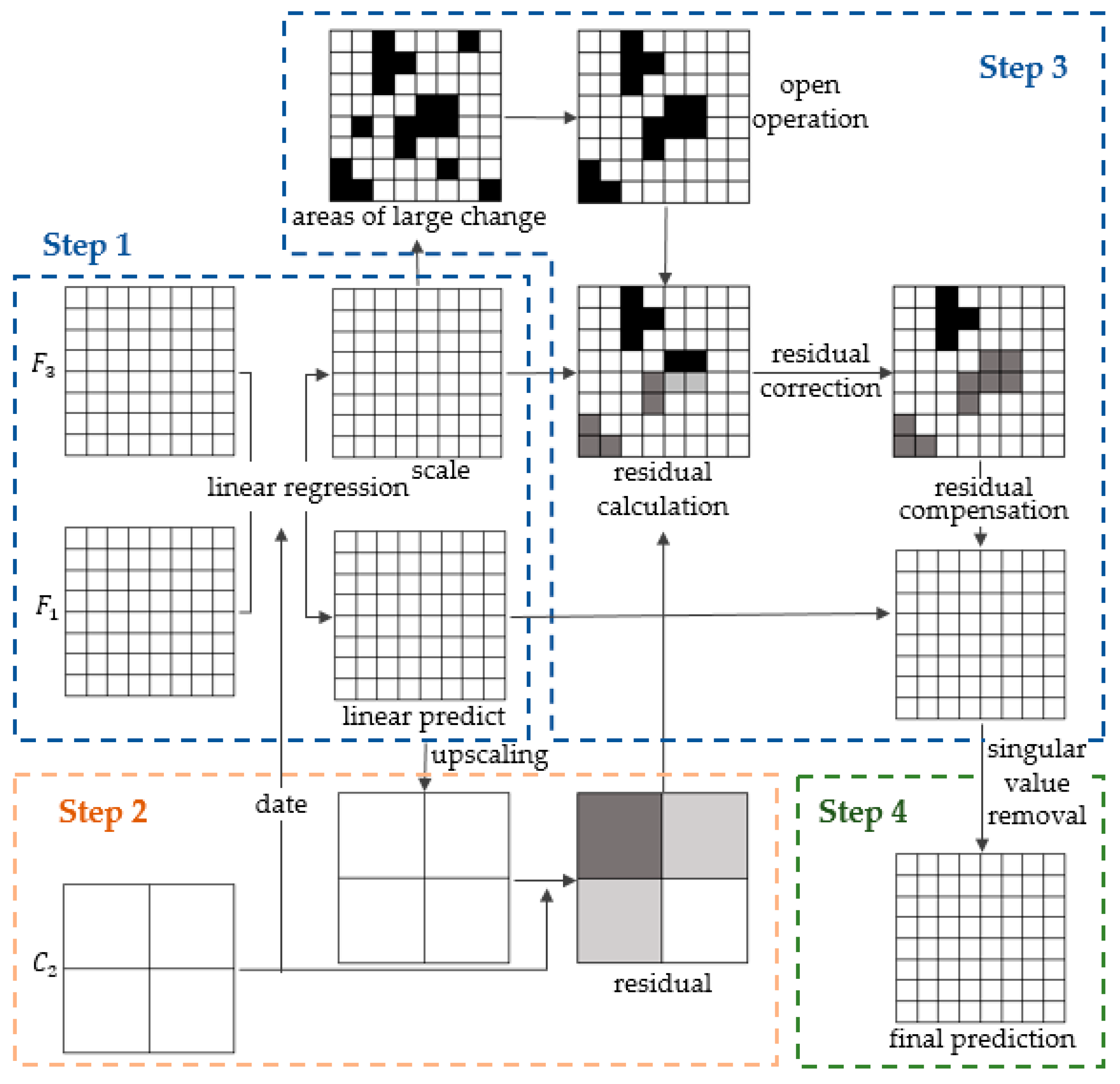
The method is divided into four steps (Figure 3). In step 1 (linear regression), the first predicted image at the prediction time () and the change slope (i.e., the regression coefficient) are generated using linear regression of the two fine resolution images at and . Step 2 (residual calculation) calculates the residual from the coarse image at and the first predicted image. Step 3 (distribution of the residual) is the key to the method in which the residual is allocated based on the change slope and assumption 1 to produce the final predicted image. The singular values in the final predicted image are further revised in step 4 (singular value correction).
Step 1. Linear Regression
With the two reference fine resolution images, the linear regression model is built for the correlation between the observed reflectance and the acquisition date for each band and each pixel to obtain the regression coefficient and the first linear predicted image at the prediction date. Here, the image of the first linear prediction is also the result of the linear interpolation prediction. The calculation is performed per-pixel without a contextual neighborhood evaluation. This enables it to provide the best capability to model local spatial variability.
The calculation of the first linear predicted image is shown in Equation (1):
where is the reflectance of pixel in band on the first predicted image at , is the reflectance of pixel in band on the fine resolution at , is the calculated change slope from the linear regression model based on the two fine reference resolution images and is the time interval from reference time to prediction time .
Step 2. Residual Calculation
The predicted coarse resolution image at time is obtained by upscaling the first predicted fine resolution image , as shown in Equation (2). That is, the reflectance of each coarse pixel is the average of all the fine pixels under its corresponding position. The residual is computed as the reflectance difference between the simulated and predicted MODIS image at (Equation (3)).
where and are the predicted and simulated coarse MODIS reflectance of the pixel in band at , respectively, and is the number of Landsat pixels used to aggregate to one MODIS pixel (here is 256). is the residual of the pixel in band at .
Step 3. Distribution of the Residual
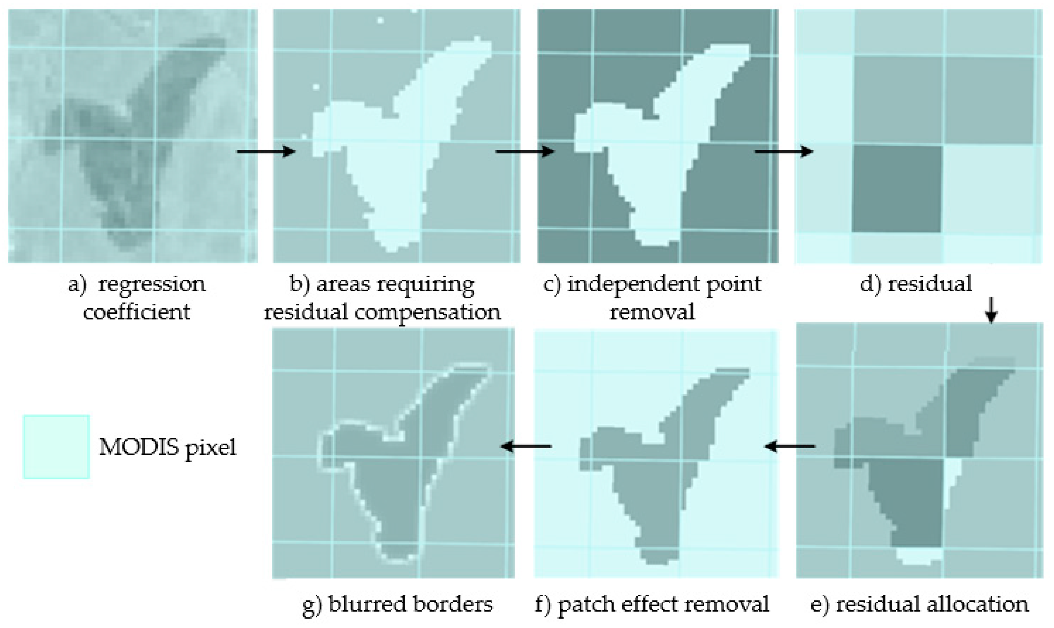
According to assumption 1, regions with a larger surface reflectance change (i.e., regions with a larger change slope) have higher prediction uncertainty, resulting in a greater residual. This means that residual compensation should be performed in these areas. For example, a positive residual means that the observed surface reflectance is larger than the predicted reflectance. Therefore, the areas with a positive change slope may need an increment to make the reflectance change faster to offset the residual, or the areas with a negative change slope may also need to be increased by an increment to make the reflectance change more slowly to offset the residual. In an extreme case, if the change slope is 0 in some areas, meaning there is barely any change in the reflectance in these areas during the study period. Therefore, the linear prediction in these areas is considered to be highly reliable and no residual distribution will take place in these areas.
In this study, approximate calculations and thresholds are used to identify the Landsat pixels with great reflectance changes in each MODIS pixel. Considering that the difference between the positive and negative changes of the surface reflectance is always large, the areas with the largest positive and negative changes (i.e., the maximum and minimum value of change) of surface reflectance are identified, respectively. Assume that the residuals that should be allocated to the two areas are and , respectively, then the calculations are as in Equations (4) and (5):
where is the residual with a 30 m spatial resolution downscaled by is the positive threshold set as half the absolute value of extremum change slope of the Landsat pixels in one MODIS pixel, is the corresponding negative threshold, and are the numbers of pixels where the slope is above and below , respectively, and and are the change slopes above and below , respectively.
There may be some independent pixels in the identified areas that need to be compensated for residuals. A morphological open operation is adopted to remove them. Because the distribution of residuals is performed on each MODIS pixel, the residuals allocated to one object composed of multiple MODIS pixels are often uneven, which leads to a patch effect. Therefore, the compensation values of each connected compensation area are averaged to eliminate the patch effect. This process is shown in Figure 4.
The final predicted fine resolution image is calculated using Equation (6):
where is the reflectance of pixel in band on the final predicted fine resolution image at prediction time .
Step 4. Singular Value Correction
Due to the approximate calculation of the residuals and some cases that do not meet the assumptions, singular values may exist after the residual compensation. This could be partly corrected by removing the single pixels that appear in the areas that need to be compensated. On the other hand, we adopted a linear increment during the study period as the extreme value of the compensation. For the areas that exceed the compensation extreme value in the final prediction results, the linear prediction results are used as replacements.
2.2.3. Comparison and Evaluation
The results of the proposed method are compared with those of the STARFM [33], FSDAF [26], and LR methods. The STARFM and FSDAF methods have different adaptability in different scenarios. With their relatively desirable prediction effect and open source code (code websites, STARFM: https://www.ars.usda.gov/; FSDAF: https://xiaolinzhu.weebly.com/open-source-code.html), they are widely used and constantly compared. The LR method here also refers to the linear interpolation method, which is based on the interpolation or the regression of the fine resolution images at two dates. The proposed method uses the residual calculated from the coarse resolution images to compensate for the linear prediction result, which improves the LR prediction results. Hence, the LR method is also used for comparison.
The performance of the ELRFM was evaluated using a variety of methods, including calculating the quantitative evaluation indicators, drawing scatter plots between the predicted and observed image on the sample points, and comparing the average of the predicted reflectance of each method at the predicted time. Quantitative assessment indicators of the root mean square error (RMSE), average difference (AD), average absolute difference (AAD), and correlation coefficient are used. These indicators are commonly adopted in many spatio–temporal fusion method studies [26,27]. The RMSE and AAD refer to the deviation and average of the absolute error between the predicted and observed reflectance, respectively. AD is used to evaluate whether the result is overestimated or underestimated as opposed to the observed reflectance. A positive AD value indicates that the predicted results are higher than the observed reflectance, while a negative AD value implies the opposite. As the proposed method is an improvement on LR, the absolute difference between the predicted and the observed reflectance of the ELRFM and LR methods is compared on every sample point.
The sample data for evaluation includes 853 points, which are randomly generated from forest land, bare land, and residential areas manually selected through visual interpretation.
In addition, to test the adaptability of the developed method to different sensors and areas, the fusion of Sentinel-2 and simulated Sentinel-3 are carried out in the other two regions. The results are also evaluated by quantitative evaluation and scatter plots.
3. Results
3.1. Comparison
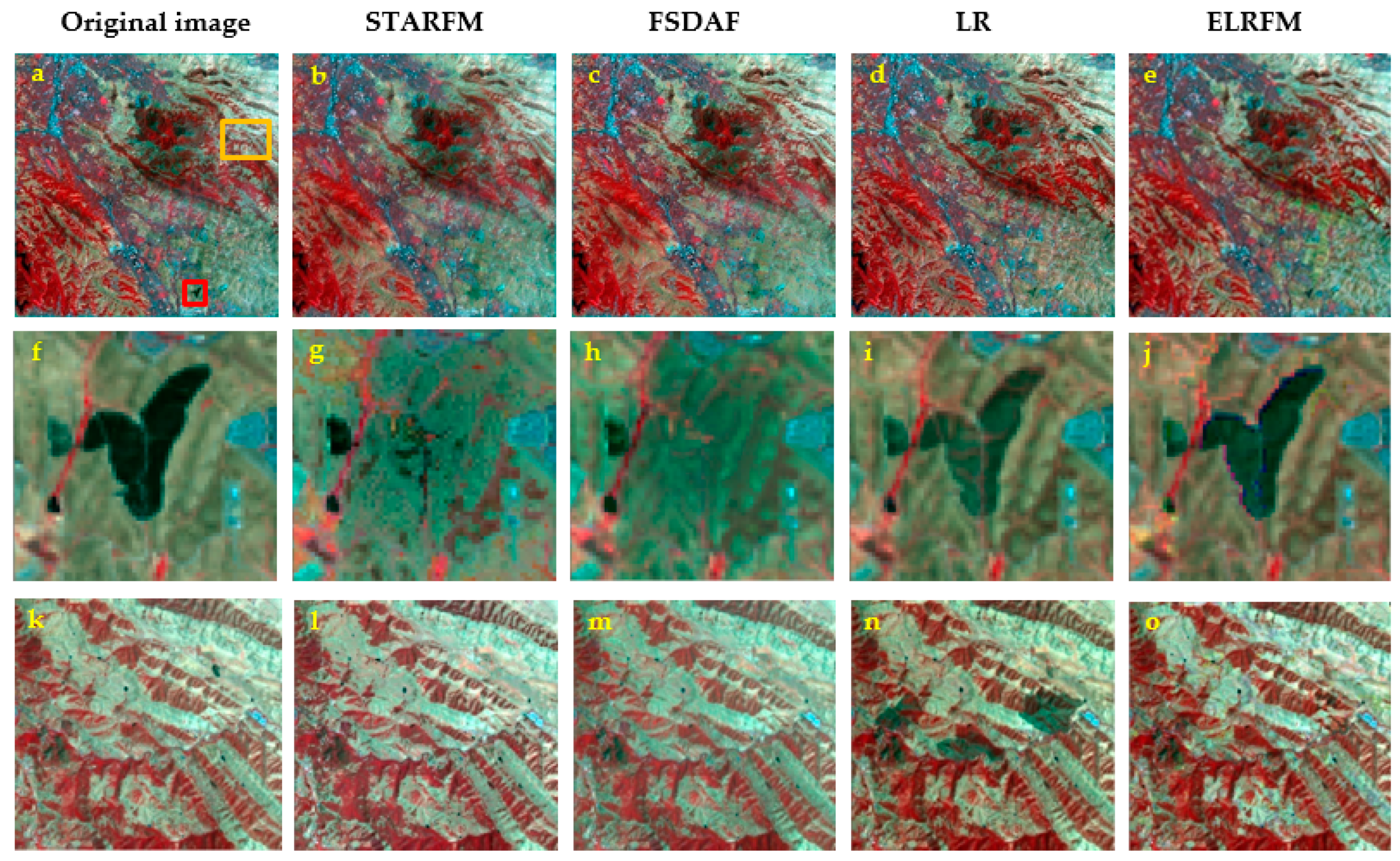
The prediction results of the STARFM, FSDAF, LR and ELRFM are shown in Figure 5. Two sub-regions of the study area are zoomed-in to show the result differences in detail between the various methods.
One sub-region is the area bounded by the red rectangle in Figure 5a. From to , a dark object appears. This feature can be identified on the fine resolution Landsat image, but it is too small to be recognized on the coarse resolution MODIS image. In reality, it exists at . The different methods are applied to determine whether the object cloud be predicted at the prediction time. The results are shown in the middle row of Figure 5. Neither the STARFM nor the FSDAF could capture this change. The linear regression method captures the feature at but with certain reflectance errors. The proposed ELRFM enhances the linear regression result and produces an image with a reflectance closest to the observed image.
The other sub-region is the area enclosed by the yellow rectangle in Figure 5a. Similar to the first sub-region, a dark object emerges in this area from to . This object is distinguishable on the Landsat image, while it is only represented by a few pixels on the MODIS image. Unlike the first sub-region, the object does not exist at . The prediction results of the four methods are shown in the bottom row of Figure 5. The result predicted by the ELRFM is comparable to that of the STARFM and FSDAF, and they are all close to the original image, while the linear regression performs the worst with the most errors.
It is worth mentioning that the STARFM and FSDAF use one pair of Landsat-MODIS images for prediction, which has advantages in regions with less cloud-free data. However, due to the reduction in effective information, the prediction accuracy is also lowered. Although it is possible to perform STARFM or FSDAF predictions on two pairs of data separately, the prediction results may show great differences, which leads to a decrease in the credibility of the comprehensive results. In addition, the operation time will be doubled when conducting prediction operations on two pairs of data.
By visual inspection, the proposed ELRFM enhances the linear regression prediction results and presents acceptable prediction results in various situations. Particularly, the ELRFM is able to capture small changes in ground objects with high prediction accuracy.
3.2. Accuracy Assessment
We calculated the quantitative indicators and drew a scatter plot between the predicted and observed reflectance for each band of the sample points. The quantitative evaluation results are shown in Table 1. It shows that the proposed ELRFM has the smallest RMSE and AAD in all bands, and in the red and near-infrared (NIR) bands, it has the lowest prediction deviation AD. However, the STARFM and FSDAF have a smaller AD in the green band. The ELRFM also has the highest correlation coefficient in each band. Overall, our method is comparable to the other three methods. Quantitative indicators show that the proposed ELRFM has less prediction deviation, and its prediction result is closer to the original image.
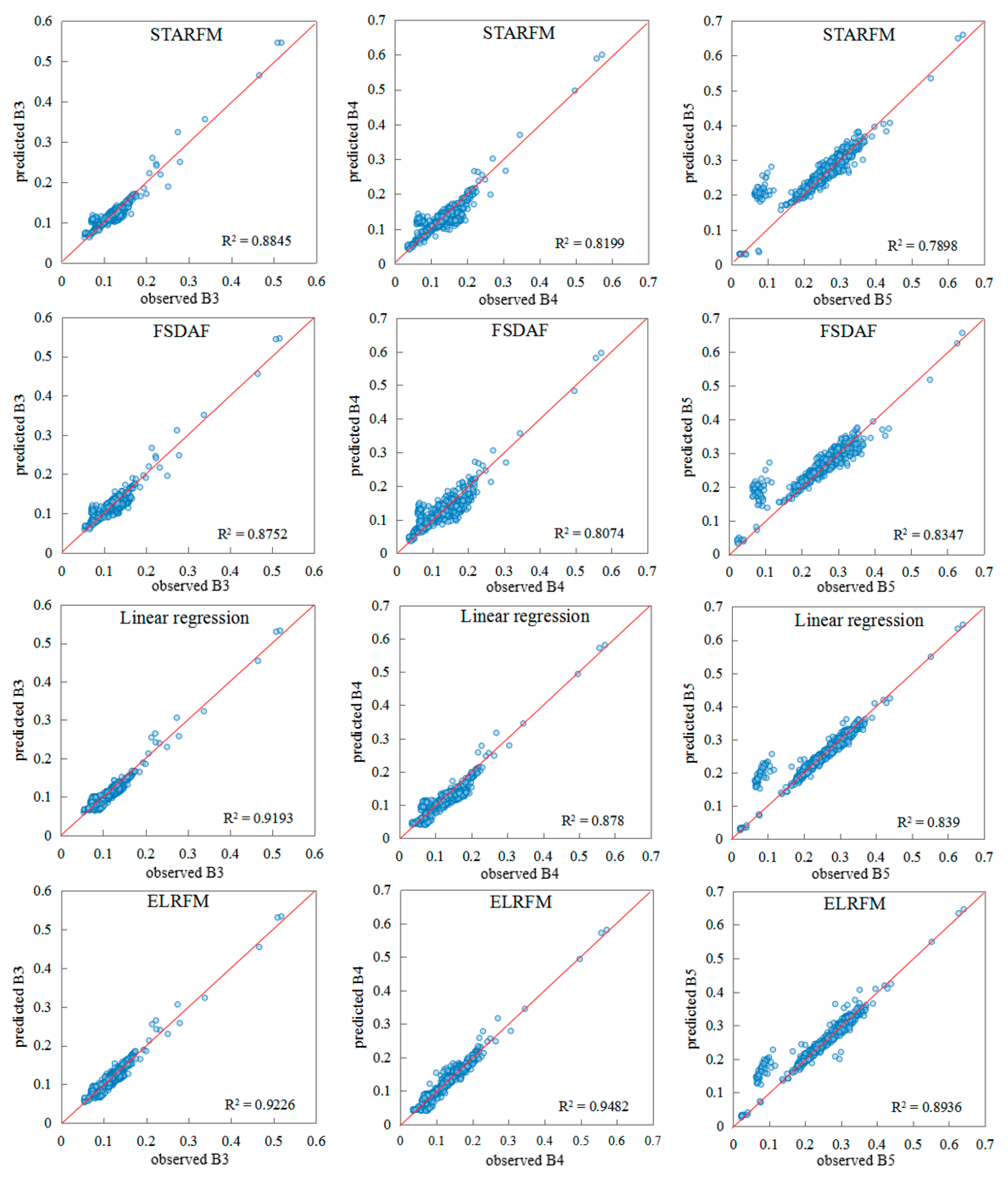
Scatter plots of the observed and the predicted reflectance from the four methods in different bands are plotted (Figure 6). It can be found that here STARFM is more accurate than FSDAF with a higher in red and green bands, while ELRFM is the most accurate of the four methods, and it exhibits an improvement over the linear regression method.
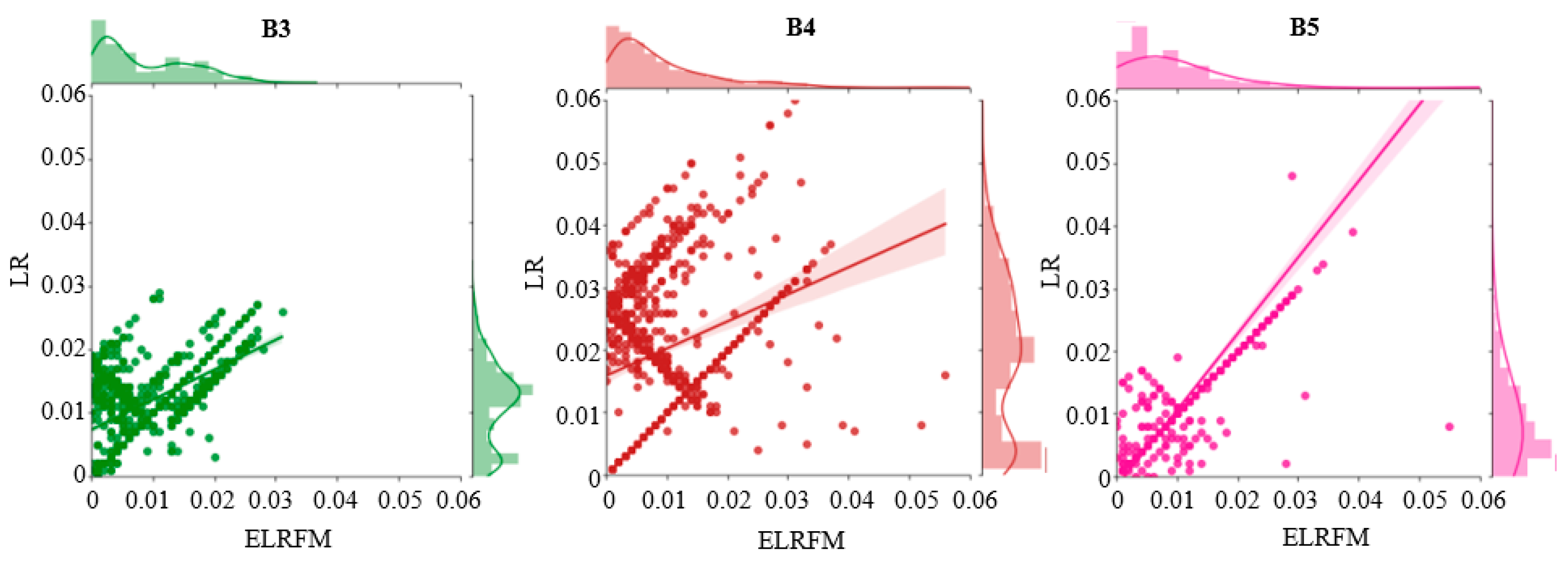
The ELRFM was also compared with LR specifically. The absolute difference between the observed and the predicted reflectance from these two methods in the green, red and NIR bands of the sample points are plotted with the corresponding histograms attached (Figure 7). The closer the point is to the origin zero, the smaller the absolute difference between the predicted and observed reflectance is, which means the greater the accuracy. From Figure 7, it can be seen that the ELRFM has more points near zero than the LR in the three bands, especially in the green and red bands, which indicates that the ELRFM performs more accurately than the LR. This conclusion could also be reached from the attached histogram, which shows that the ELRFM histograms are positively skewed and the LR histograms are more flattened and spread out.
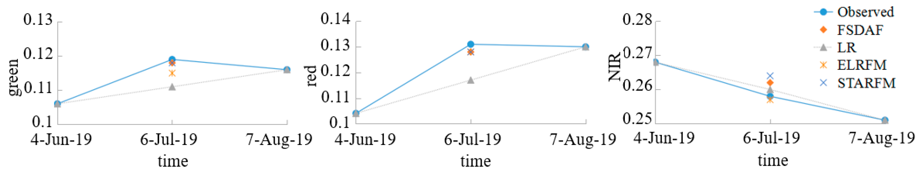
Figure 8 shows the average of the observed and predicted reflectance from the four fusion methods in different bands. In the green band, the STARFM and FSDAF are closer to the observed average reflectance than the ELRFM and LR. In the red band, the ELRFM, STARFM, and FSDAF are similarly close to the observed reflectance, while LR is farther away. In the NIR band, among the four methods, the ELRFM is the closest to the observed average reflectance.
3.3. Further Verification
To investigate whether the proposed ELRFM could also perform well in different areas and using different sensors, two other test areas were selected. One site (zone 1) is located near Hatton in Adams County, Washington, United States (Lat/Lng: 46.81/−118.92), which is dominated by cropland and bare land. The other site (zone 2) is located in a section of Green River, Wyoming (Lat/Lng: 42.06/−110.12), United States. This area is dominated by water and shrubs. Sentinel-2 (10 m spatial resolution for green, red and NIR bands) and Sentinel-3 (300 m spatial resolution) data are selected as the fine and coarse resolution images, respectively, for the fusion experiment. Sentinel-2 used here is the level-1C orthorectified TOA reflectance data from GEE. Similarly, to avoid the interference caused by the radiometric or geometric inconsistencies between the two sensors, the simulated Sentinel-3 (also called Sentinel-3-like) images are aggregated from the Sentinel-2 images. For zone 1, the fine–coarse image pairs (i.e., Sentinel-2 and simulated Sentinel-3) acquired on 29 May and 3 July 2020, respectively, and the simulated Sentinel-3 image acquired on 18 June 2020 are used to predict the Sentinel-2-like image of 18 June 2020. For zone 2, the fine–coarse image pairs acquired on 13 May and 12 July 2019, respectively, and the Sentinel-3-like image from 12 June 2019 are used to predict the Sentinel-2-like image of 12 June 2019. The images used in zone 1 and zone 2 are shown in Figures S1 and S2 of the Supplementary Material.
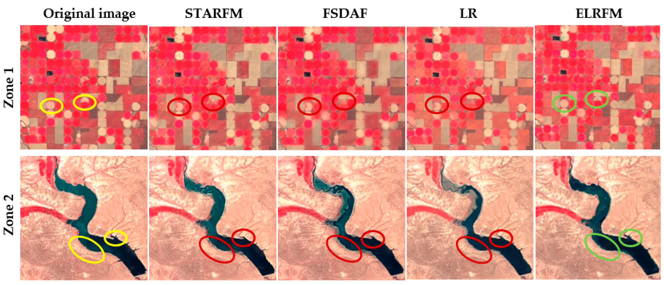
The fusion results from different methods are shown in Figure 9. In zone 1, ELRFM achieves a similar result to that of STARFM and FSDAF methods, while it is superior to detect the feature type changes in some areas. For example, in the yellow ellipses of the original image, the ELRFM detects the transition between the crops and the bare land. In zone 2, the ELRFM works better where the water area changes significantly. For example, in the yellow ellipses shown in the original image, the ELRFM predicts the water body more accurately than the other methods. The boundaries of the water are almost within one coarse pixel, which shows that the ELRFM has the advantage of being able to predict small LULC type changes within one coarse pixel. Moreover, the tests in zone 1 and 2 illustrate that the ELRFM cloud works well even when the fine resolution and the coarse resolution differ by 30 times.
In addition, 599 and 700 sample points are randomly generated in zone 1 and 2, respectively, for quantitative evaluation and scatter plot drawing. The results are shown in Table S1, Figures S3 and S4 of the Supplementary Materials.
4. Discussion
Unlike the STARFM and FSDAF methods that use similar pixels to predict reflectance, ELRFM builds a linear model for each pixel. Therefore, it is able to preserve spatial detail. In addition, ELRFM is more computationally efficient than STARFM and FSDAF, as it is based on the GEE platform and uses GEE’s cloud computing capability.
The proposed method also has certain limitations. It is not always better than the STARFM and FSDAF methods at predicting the reflectance. The scatter plots of the observed and predicted reflectance of zone 1 (see Figure S3) show that the ELRFM is inferior to STARFM and FSDAF, with a lower (e.g., for the green band, ELRFM vs. STARFM and FSDAF: 0.6526 vs. 0.8044 and 0.7999). From the quantitative evaluation results of zone 1 (see Table S1), ELRFM only predicts the lowest RMSE (ELRFM vs. STARFM, FSDAF, and LR: 171.61 vs. 183.75, 172.69 and 282.56) and a higher (0.96 vs. 0.95, 0.96 and 0.92) in the red band with slight advantages. In the prediction of the green and NIR bands, the FSDAF has the smallest RMSE. In all three bands, the predicted result from the STARFM has the smallest AAD. The above evaluation results show that the STARFM and FSDAF methods perform better than the ELRFM. This is because zone 1 is mainly faced with surface reflectance changes rather than LULC changes. The STARFM and FSDAF methods are advantageous in this case.
The observed and predicted reflectance scatter plots of zone 2 (see Figure S4), where some areas experienced LULC type changes, show that the ELRFM is superior to the STARFM and FSDAF methods by predicting the highest in all three bands. Taking the green band as an example, the of the ELRFM is 0.951, while those of the STARFM, FSDAF, and LR methods are 0.5913, 0.8716 and 0.9368, respectively. The quantitative evaluation index results of the four methods in zone 2 are shown in Table S1. In this zone, the RMSE and AAD of the ELRFM in the three bands are the smallest (e.g., in the green band, ELRFM vs. STARFM, FSDAF, and LR, RMSE: 111.07 vs. 146.23, 173.67 and 123.66; AAD: 67.27 vs. 75.14, 102.14 and 71.46) and the is the largest (0.98 vs. 0.96, 0.93 and 0.97), which shows that the ELRFM has the best prediction accuracy in zone 2. This is because LULC changes occurred in many parts of this region, and the ELRFM is based on the linear regression of each pixel, which can better capture this change.
Developing generic fusion algorithms suitable for all types of scenarios and applications remains an open problem. In general, the ELRFM is advantageous in monitoring the changes in surface feature categories. Therefore, it could be used in applications focused on surface feature changes, such as water monitoring. For applications that focus on changes in surface reflectance, such as crop growth, the STARFM and FSDAF methods are a better choice.
The algorithm proposed in this paper is an improvement on the linear fitting method, and it generally more accurate than the linear method. However, due to the statistical calculation and compensation of the residual error within each coarse pixel, the ELRFM has a plate effect on the coarse pixels scale. In addition, a fixed threshold strategy in determining the degree of change also has certain limitations. Further research could be conducted on automatic threshold determination based on the statistical information in the coarse pixels. As data acquisition and processing become easier, further work could also focus on the comprehensive use of time series information to aid data spatio–temporal fusion. For example, a time series could be used to make preliminary predictions and then compensate for residuals.
5. Conclusions
Dense daily time series Earth observation data are important for surface monitoring. However, they are currently not freely available. Therefore, data fusion methods can be applied to generate synthetic high-resolution and dense images. In this paper, we developed an efficient spatio–temporal fusion model, ELRFM, based on linear regression. This method compensates for the residual error between the linear regression prediction results and the actual coarse resolution image with a regression coefficient.
The ELRFM maintains spatial details and presents a better ability to capture small feature changes at the fine image scale compared with the spatial and temporal adaptive reflectance fusion model (STARFM) and the flexible spatio–temporal data fusion (FSDAF) method. In addition, it is more computationally efficient than the STARFM and FSDAF due to the simple design and implementation on the Google Earth Engine platform. The ELRFM is applicable not only to the fusion of Landsat and the moderate resolution imaging spectroradiometer (MODIS), but also to the fusion of Sentinel-2 and Sentinel-3. However, since the ELRFM is based on certain assumptions and the residual compensation process in it is an approximate calculation, the prediction accuracy will not be high in cases that do not meet these assumptions. For example, a longer study period will result in lower prediction accuracy, because the land-use/land-cover types do not typically show linear changes over a long period. Overall, the proposed method is typically more accurate than the linear fitting method, and, in some cases (such as feature type changes in the coarse pixel), outperforms the existing STARFM and FSDAF methods. The ELRFM could be used as a supplement for the spatio–temporal fusion algorithm community.
The method proposed performs well on the fusion of simulated data. Future research could consider its testing and application in real scenarios. In addition, with more satellite launches and an increasing number of freely available medium and high-resolution images, future research may include other higher spatial resolution data such as Gaofen-1 wide field of view (GF-1 WFV) sensor, which became free in 2019. These data have a higher temporal resolution (a 2-day revisit cycle) than Landsat and presents a great potential for time series applications.
Supplementary Materials
The following are available online at https://0-www-mdpi-com.brum.beds.ac.uk/2072-4292/12/23/3900/s1, Figure S1: Color composited images (RGB: near-infrared, red, green) of zone 1. (a–c) are Sentinel-2 images acquired on May 29, June 18, and July 3, 2020, respectively (1230 × 1200 pixels with 10 m resolution), and (d–f) are Sentinel-3 like images aggregated from (a–c), Figure S2: Color composited images (RGB: near-infrared, red, green) of zone 2. (a–c) are Sentinel-2 images acquired on May 13, June 12, and July 12, 2019, respectively (1530 × 1500 pixels with 10m resolution), and (d–f) are Sentinel-3 like images aggregated from (a–c), Figure S3: Scatter plots of the observed and predicted reflectance of zone 1 from the four data fusion methods in green (B3), red (B4), and near-infrared (B8) bands, respectively, Figure S4: Scatter plots of the observed and predicted reflectance of zone 2 from the four data fusion methods in green (B3), red (B4), and near-infrared (B8) bands, respectively, Table S1: Accuracy assessment results of the four data fusion methods. Root mean square error (RMSE), average difference (AD), average absolute difference (AAD), and correlation coefficient r, near-infrared (NIR).
Author Contributions
Conceptualization, B.B. and Y.T.; methodology, B.B., G.D. and A.W.; software, B.B.; validation, A.W., G.D. and A.H.; formal analysis, B.B., Y.T. and A.W.; investigation, B.B., G.D. and A.H.; writing—original draft preparation, B.B.; writing—review and editing, A.W., G.D. and A.H.; supervision, Y.T., A.W.; funding acquisition, Y.T. All authors have read and agreed to the published version of the manuscript.
Funding
This work was supported by the Project for Construction of Comprehensive Management Network Software and Spatial Information Service Platform in The Three Gorges Reservoir Area (grant number 2017HXNL-01), National Key R&D Program of China (No. 2019YFE0126400) and the China Scholarship Council.
Acknowledgments
We would like to thank all the reviewers for their helpful and constructive comments on this paper. We also would like to thank the authors of the STARFM and FSDAF algorithms for publishing the code.
Conflicts of Interest
The authors declare no conflict of interest.
References
- Kovalskyy, V.; Roy, D.P. The global availability of Landsat 5 TM and Landsat 7 ETM+ land surface observations and implications for global 30m Landsat data product generation. Remote Sens. Environ. 2013, 130, 280–293. [Google Scholar] [CrossRef] [Green Version]
- Drusch, M.; Del Bello, U.; Carlier, S.; Colin, O.; Fernandez, V.M.; Gascon, F.; Hoersch, B.; Isola, C.; Laberinti, P.; Martimort, P.; et al. Sentinel-2: ESA’s Optical High-Resolution Mission for GMES Operational Services. Remote Sens. Environ. 2012, 120, 25–36. [Google Scholar] [CrossRef]
- Pekel, J.-F.; Cottam, A.; Gorelick, N.; Belward, A.S. High-resolution mapping of global surface water and its long-term changes. Nature 2016, 540, 418–422. [Google Scholar] [CrossRef] [PubMed]
- Hansen, M.C.; Potapov, P.V.; Moore, R.; Hancher, M.; Turubanova, S.A.; Tyukavina, A.; Thau, D.; Stehman, S.V.; Goetz, S.J.; Loveland, T.R.; et al. High-Resolution Global Maps of 21st-Century Forest Cover Change. Science 2013, 342, 850–854. [Google Scholar] [CrossRef] [PubMed] [Green Version]
- Donchyts, G.; Schellekens, J.; Winsemius, H.; Eisemann, E.; Van De Giesen, N. A 30 m Resolution Surface Water Mask Including Estimation of Positional and Thematic Differences Using Landsat 8, SRTM and OpenStreetMap: A Case Study in the Murray-Darling Basin, Australia. Remote Sens. 2016, 8, 386. [Google Scholar] [CrossRef] [Green Version]
- Donchyts, G.; Baart, F.; Winsemius, H.; Gorelick, N.; Kwadijk, J.; Van De Giesen, N. Earth’s surface water change over the past 30 years. Nat. Clim. Chang. 2016, 6, 810–813. [Google Scholar] [CrossRef]
- Gorelick, N.; Hancher, M.; Dixon, M.; Ilyushchenko, S.; Thau, D.; Moore, R. Google Earth Engine: Planetary-scale geospatial analysis for everyone. Remote Sens. Environ. 2017, 202, 18–27. [Google Scholar] [CrossRef]
- Rudiyanto; Minasny, B.; Shah, R.M.; Soh, N.C.; Arif, C.; Setiawan, B.I. Automated Near-Real-Time Mapping and Monitoring of Rice Extent, Cropping Patterns, and Growth Stages in Southeast Asia Using Sentinel-1 Time Series on a Google Earth Engine Platform. Remote Sens. 2019, 11, 1666. [Google Scholar] [CrossRef] [Green Version]
- Carrasco, L.; O’Neil, A.W.; Morton, R.D.; Rowland, C.S. Evaluating Combinations of Temporally Aggregated Sentinel-1, Sentinel-2 and Landsat 8 for Land Cover Mapping with Google Earth Engine. Remote Sens. 2019, 11, 288. [Google Scholar] [CrossRef] [Green Version]
- Bai, B.; Tan, Y.; Guo, D.; Xu, B. Dynamic Monitoring of Forest Land in Fuling District Based on Multi-Source Time Series Remote Sensing Images. ISPRS Int. J. Geo-Inf. 2019, 8, 36. [Google Scholar] [CrossRef] [Green Version]
- Liu, X.; Shi, Z.; Huang, G.; Bo, Y.; Chen, G. Time series remote sensing data-based identification of the dominant factor for inland lake surface area change: Anthropogenic activities or natural events? Remote Sens. 2020, 12, 612. [Google Scholar] [CrossRef] [Green Version]
- Teluguntla, P.; Thenkabail, P.; Oliphant, A.; Xiong, J.; Gumma, M.K.; Congalton, R.G.; Yadav, K.; Huete, A. A 30-m landsat-derived cropland extent product of Australia and China using random forest machine learning algorithm on Google Earth Engine cloud computing platform. ISPRS J. Photogramm. Remote Sens. 2018, 144, 325–340. [Google Scholar] [CrossRef]
- Verdoliva, L.; Gaetano, R.; Ruello, G.; Poggi, G. Optical-Driven Nonlocal SAR Despeckling. IEEE Geosci. Remote Sens. Lett. 2015, 12, 314–318. [Google Scholar] [CrossRef]
- Rao, P.; Jiang, W.; Hou, Y.; Chen, Z.; Jia, K. Dynamic Change Analysis of Surface Water in the Yangtze River Basin Based on MODIS Products. Remote Sens. 2018, 10, 1025. [Google Scholar] [CrossRef] [Green Version]
- Shen, H.; Huang, L.; Zhang, L.; Wu, P.; Zeng, C. Long-term and fine-scale satellite monitoring of the urban heat island effect by the fusion of multi-temporal and multi-sensor remote sensed data: A 26-year case study of the city of Wuhan in China. Remote Sens. Environ. 2016, 172, 109–125. [Google Scholar] [CrossRef]
- D’Addabbo, A.; Refice, A.; Pasquariello, G.; Lovergine, F. SAR/optical data fusion for flood detection. In Proceedings of the 2016 IEEE International Geoscience and Remote Sensing Symposium (IGARSS), Beijing, China, 10–15 July 2016; pp. 7631–7634. [Google Scholar]
- Torbick, N.; Chowdhury, D.; Salas, W.; Qi, J. Monitoring Rice Agriculture across Myanmar Using Time Series Sentinel-1 Assisted by Landsat-8 and PALSAR-2. Remote Sens. 2017, 9, 119. [Google Scholar] [CrossRef] [Green Version]
- You, N.; Dong, J. Examining earliest identifiable timing of crops using all available Sentinel 1/2 imagery and Google Earth Engine. ISPRS J. Photogramm. Remote Sens. 2020, 161, 109–123. [Google Scholar] [CrossRef]
- Ghosh, R.; Gupta, P.K.; Tolpekin, V.; Srivastav, S.K. An enhanced spatiotemporal fusion method—Implications for coal fire monitoring using satellite imagery. Int. J. Appl. Earth Obs. Geoinf. 2020, 88, 102056. [Google Scholar] [CrossRef]
- Zhu, X.; Cai, F.; Tian, J.; Williams, T.K.A. Spatiotemporal Fusion of Multisource Remote Sensing Data: Literature Survey, Taxonomy, Principles, Applications, and Future Directions. Remote Sens. 2018, 10, 527. [Google Scholar] [CrossRef] [Green Version]
- Moreno-martínez, Á.; Izquierdo-verdiguier, E.; Maneta, M.P.; Camps-valls, G.; Robinson, N.; Muñoz-marí, J.; Sedano, F.; Clinton, N.; Running, S.W. Remote Sensing of Environment Multispectral high resolution sensor fusion for smoothing and gap-filling in the cloud. Remote Sens. Environ. 2020, 247, 111901. [Google Scholar] [CrossRef]
- Laborde, H.; Douzal, V.; Piña, H.A.R.; Morand, S.; Cornu, J.-F. Landsat-8 cloud-free observations in wet tropical areas: A case study in South East Asia. Remote Sens. Lett. 2017, 8, 537–546. [Google Scholar] [CrossRef]
- Ghassemian, H. A review of remote sensing image fusion methods. Inf. Fusion 2016, 32, 75–89. [Google Scholar] [CrossRef]
- Luo, Y.; Guan, K.; Peng, J. STAIR: A generic and fully-automated method to fuse multiple sources of optical satellite data to generate a high-resolution, daily and cloud-/gap-free surface reflectance product. Remote Sens. Environ. 2018, 214, 87–99. [Google Scholar] [CrossRef]
- Chen, B.; Chen, L.; Huang, B.; Michishita, R.; Xu, B. Dynamic monitoring of the Poyang Lake wetland by integrating Landsat and MODIS observations. ISPRS J. Photogramm. Remote Sens. 2018, 139, 75–87. [Google Scholar] [CrossRef]
- Zhu, X.; Helmer, E.H.; Gao, F.; Liu, D.; Chen, J.; Lefsky, M.A. A flexible spatiotemporal method for fusing satellite images with different resolutions. Remote Sens. Environ. 2016, 172, 165–177. [Google Scholar] [CrossRef]
- Li, X.; Foody, G.M.; Boyd, D.S.; Ge, Y.; Zhang, Y.; Du, Y.; Ling, F. SFSDAF: An enhanced FSDAF that incorporates sub-pixel class fraction change information for spatio-temporal image fusion. Remote Sens. Environ. 2020, 237, 111537. [Google Scholar] [CrossRef]
- Rao, Y.; Zhu, X.; Chen, J.; Wang, J. An Improved Method for Producing High Spatial-Resolution NDVI Time Series Datasets with Multi-Temporal MODIS NDVI Data and Landsat TM/ETM+ Images. Remote Sens. 2015, 7, 7865–7891. [Google Scholar] [CrossRef] [Green Version]
- Kimm, H.; Guan, K.; Jiang, C.; Peng, B.; Gentry, L.F.; Wilkin, S.C.; Wang, S.; Cai, Y.; Bernacchi, C.J.; Peng, J.; et al. Deriving high-spatiotemporal-resolution leaf area index for agroecosystems in the U.S. Corn Belt using Planet Labs CubeSat and STAIR fusion data. Remote Sens. Environ. 2020, 239, 111615. [Google Scholar] [CrossRef]
- Long, D.; Yan, L.; Bai, L.; Zhang, C.; Li, X.; Lei, H.; Yang, H.; Tian, F.; Zeng, C.; Meng, X.; et al. Generation of MODIS-like land surface temperatures under all-weather conditions based on a data fusion approach. Remote Sens. Environ. 2020, 246, 111863. [Google Scholar] [CrossRef]
- Yin, Z.; Wu, P.; Foody, G.M.; Wu, Y.; Liu, Z.; Du, Y.; Ling, F. Spatiotemporal Fusion of Land Surface Temperature Based on a Convolutional Neural Network. IEEE Trans. Geosci. Remote Sens. 2020, 1–15. [Google Scholar] [CrossRef]
- Xie, D.; Zhang, J.; Zhu, X.; Pan, Y.; Liu, H.; Yuan, Z.; Yun, Y. An Improved STARFM with Help of an Unmixing-Based Method to Generate High Spatial and Temporal Resolution Remote Sensing Data in Complex Heterogeneous Regions. Sensors 2016, 16, 207. [Google Scholar] [CrossRef] [PubMed] [Green Version]
- Gao, F.; Masek, J.; Schwaller, M.; Hall, F. On the Blending of the MODIS and Landsat ETM + Surface Reflectance: Predicting Daily Landsat Surface Reflectanc. IEEE Trans. Geosci. Remote Sens. 2006, 44, 2207–2218. [Google Scholar]
- Hilker, T.; Wulder, M.A.; Coops, N.C.; Linke, J.; McDermid, G.; Masek, J.G.; Gao, F.; White, J.C. A new data fusion model for high spatial- and temporal-resolution mapping of forest disturbance based on Landsat and MODIS. Remote Sens. Environ. 2009, 113, 1613–1627. [Google Scholar] [CrossRef]
- Liu, X.; Deng, C.; Chanussot, J.; Hong, D.; Zhao, B. StfNet: A two-stream convolutional neural network for spatiotemporal image fusion. IEEE Trans. Geosci. Remote Sens. 2019, 57, 6552–6564. [Google Scholar] [CrossRef]
- Zhu, X.; Chen, J.; Gao, F.; Chen, X.; Masek, J.G. An enhanced spatial and temporal adaptive reflectance fusion model for complex heterogeneous regions. Remote Sens. Environ. 2010, 114, 2610–2623. [Google Scholar] [CrossRef]
- Weng, Q.; Fu, P.; Gao, F. Generating daily land surface temperature at Landsat resolution by fusing Landsat and MODIS data. Remote Sens. Environ. 2014, 145, 55–67. [Google Scholar] [CrossRef]
- Knauer, K.; Gessner, U.; Fensholt, R.; Kuenzer, C. An ESTARFM Fusion Framework for the Generation of Large-Scale Time Series in Cloud-Prone and Heterogeneous Landscapes. Remote Sens. 2016, 8, 425. [Google Scholar] [CrossRef] [Green Version]
- Wang, Q.; Atkinson, P.M. Spatio-temporal fusion for daily Sentinel-2 images. Remote Sens. Environ. 2018, 204, 31–42. [Google Scholar] [CrossRef] [Green Version]
- Emelyanova, I.V.; McVicar, T.R.; Van Niel, T.G.; Li, L.T.; Van Dijk, A.I.J.M. Assessing the accuracy of blending Landsat—MODIS surface reflectances in two landscapes with contrasting spatial and temporal dynamics: A framework for algorithm selection. Remote Sens. Environ. 2013, 133, 193–209. [Google Scholar] [CrossRef]
- Liu, M.; Yang, W.; Zhu, X.; Chen, J.; Chen, X.; Yang, L.; Helmer, E.H. An Improved Flexible Spatiotemporal DAta Fusion (IFSDAF) method for producing high spatiotemporal resolution normalized difference vegetation index time series. Remote Sens. Environ. 2019, 227, 74–89. [Google Scholar] [CrossRef]
- Gevaert, C.M.; García-Haro, F.J. A comparison of STARFM and an unmixing-based algorithm for Landsat and MODIS data fusion. Remote Sens. Environ. 2015, 156, 34–44. [Google Scholar] [CrossRef]
Figure 1.
Schema of the enhanced linear regression spatio–temporal fusion method (ELRFM). /, /, and / indicate fine/coarse resolution images at , , and , respectively.
Figure 1.
Schema of the enhanced linear regression spatio–temporal fusion method (ELRFM). /, /, and / indicate fine/coarse resolution images at , , and , respectively.

Figure 2.
Color composited images (RGB: near-infrared, red, green) of the study area. (a–c) are the Landsat 8 images acquired on 4 June, 6 July and 7 August 2019, respectively (960 × 960 pixels with a 30 m resolution), and (d–f) are moderate resolution imaging spectroradiometer (MODIS) images (480 m resolution) aggregated from (a–c).

Figure 3.
Flowchart of the ELRFM.

Figure 4.
Residual distribution process.

Figure 5.
Color composited image (RGB: near-infrared, red, green) results from four spatio–temporal fusion methods: (a) reference image at ; (b) spatial and temporal adaptive reflectance fusion model (STARFM); (c) flexible spatio–temporal data fusion method (FSDAF); (d) linear regression (LR); (e) ELRFM. The images at (f–j) and (k–o) are the corresponding zoomed-in sub-region images bounded by the red and yellow rectangles in (a), respectively.

Figure 6.
Scatter plots of the observed and predicted reflectance from the four fusion methods in the green (B3), red (B4), and near-infrared (B5) bands.
Figure 6.
Scatter plots of the observed and predicted reflectance from the four fusion methods in the green (B3), red (B4), and near-infrared (B5) bands.

Figure 7.
Distribution of the absolute difference between the observed and predicted reflectance from the LR and ELRFM in the green (B3), red (B4), and near-infrared (B5) bands.
Figure 7.
Distribution of the absolute difference between the observed and predicted reflectance from the LR and ELRFM in the green (B3), red (B4), and near-infrared (B5) bands.

Figure 8.
Average of the observed and predicted reflectance of the four methods in the green, red, and near-infrared (NIR) bands.
Figure 8.
Average of the observed and predicted reflectance of the four methods in the green, red, and near-infrared (NIR) bands.

Figure 9.
Comparison of the original Sentinel-2 image (near infrared, red, green bands as RGB) and the predictions of different fusion methods for the other two test areas.
Figure 9.
Comparison of the original Sentinel-2 image (near infrared, red, green bands as RGB) and the predictions of different fusion methods for the other two test areas.


Table 1.
Quantitative assessment results of the four data fusion methods. Root mean square error (RMSE), average difference (AD), average absolute difference (AAD), and correlation coefficient , near-infrared (NIR).
Table 1.
Quantitative assessment results of the four data fusion methods. Root mean square error (RMSE), average difference (AD), average absolute difference (AAD), and correlation coefficient , near-infrared (NIR).
| Methods | Band | RMSE | AAD | AD | |
|---|---|---|---|---|---|
| STARFM | Green | 0.0123 | 0.0084 | −0.0003 | 0.9405 |
| Red | 0.0217 | 0.0147 | −0.0021 | 0.9054 | |
| NIR | 0.0344 | 0.0176 | 0.0081 | 0.8886 | |
| FSDAF | Green | 0.0128 | 0.0091 | −0.0005 | 0.9357 |
| Red | 0.0224 | 0.0157 | −0.0022 | 0.8985 | |
| NIR | 0.0312 | 0.0177 | 0.0056 | 0.9136 | |
| LR | Green | 0.0127 | 0.0107 | −0.0074 | 0.9589 |
| Red | 0.0221 | 0.0181 | −0.0131 | 0.9372 | |
| NIR | 0.0299 | 0.0145 | 0.0033 | 0.9159 | |
| ELRFM | Green | 0.0112 | 0.0084 | −0.0039 | 0.9605 |
| Red | 0.0123 | 0.0091 | −0.0021 | 0.9738 | |
| NIR | 0.0244 | 0.0131 | 0.0013 | 0.9453 |
The bold numbers indicate the results with the best accuracy.
Publisher’s Note: MDPI stays neutral with regard to jurisdictional claims in published maps and institutional affiliations. |
© 2020 by the authors. Licensee MDPI, Basel, Switzerland. This article is an open access article distributed under the terms and conditions of the Creative Commons Attribution (CC BY) license (http://creativecommons.org/licenses/by/4.0/).
Share and Cite
MDPI and ACS Style
Bai, B.; Tan, Y.; Donchyts, G.; Haag, A.; Weerts, A. A Simple Spatio–Temporal Data Fusion Method Based on Linear Regression Coefficient Compensation. Remote Sens. 2020, 12, 3900. https://0-doi-org.brum.beds.ac.uk/10.3390/rs12233900
AMA Style
Bai B, Tan Y, Donchyts G, Haag A, Weerts A. A Simple Spatio–Temporal Data Fusion Method Based on Linear Regression Coefficient Compensation. Remote Sensing. 2020; 12(23):3900. https://0-doi-org.brum.beds.ac.uk/10.3390/rs12233900
Chicago/Turabian StyleBai, Bingxin, Yumin Tan, Gennadii Donchyts, Arjen Haag, and Albrecht Weerts. 2020. "A Simple Spatio–Temporal Data Fusion Method Based on Linear Regression Coefficient Compensation" Remote Sensing 12, no. 23: 3900. https://0-doi-org.brum.beds.ac.uk/10.3390/rs12233900
Note that from the first issue of 2016, this journal uses article numbers instead of page numbers. See further details here.