Article

Optimizing Near Real-Time Detection of Deforestation on Tropical Rainforests Using Sentinel-1 Data

Remote Sensing Division, Instituto Nacional de Pesquisas Espaciais (INPE), São José dos Campos 12227-010, Brazil
*
Author to whom correspondence should be addressed.
Remote Sens. 2020, 12(23), 3922; https://0-doi-org.brum.beds.ac.uk/10.3390/rs12233922
Submission received: 8 October 2020 / Revised: 27 October 2020 / Accepted: 29 October 2020 / Published: 30 November 2020
(This article belongs to the Section Environmental Remote Sensing)

Abstract

:
Early Warning Systems (EWS) for near real-time detection of deforestation are a fundamental component of public policies focusing on the reduction in forest biomass loss and associated CO2 emissions. Most of the operational EWS are based on optical data, which are severely limited by the cloud cover in tropical environments. Synthetic Aperture Radar (SAR) data can help to overcome this observational gap. SAR measurements, however, can be altered by atmospheric effects on and variations in surface moisture. Different techniques of time series (TS) stabilization have been used to mitigate the instability of C-band SAR measurements. Here, we evaluate the performance of two different approaches to SAR TS stabilization, harmonic deseasonalization and spatial stabilization, as well as two deforestation detection techniques, Adaptive Linear Thresholding (ALT) and maximum likelihood classification (MLC). We set up a rigorous, Amazon-wide validation experiment using the Google Earth Engine platform to sample and process Sentinel-1A data of nearly 6000 locations in the whole Brazilian Amazonian basin, generating more than 8M processed samples. Half of those locations correspond to non-degraded forest areas, while the other half pertained to 2019 deforested areas. The detection results showed that the spatial stabilization algorithm improved the results of the MLC approach, reaching 94.36% global accuracy. The ALT detection algorithm performed better, reaching 95.91% global accuracy, regardless of the use of any stabilization method. The results of this experiment are being used to develop an operational EWS in the Brazilian Amazon.

Graphical Abstract

1. Introduction

The latest world data on primary forest losses in tropical regions report a 3.8 Mha loss in 2019, where Brazil accounts for one third of this loss, reaching 1.36 MHa of deforested area [1]. The most recent official data from the Brazilian government reveal a significant recent rise in annual rates of deforestation, from 0.75 Mha·yr−1 (2018) to 1.01 MHa·yr−1 (2019), which is an increment of 34% in a single year [2].
In this rapid degrading scenario, Early Warning Systems (EWS), defined as a collection of algorithms and procedures able to identify tree loss or disturbance, on a periodic basis (monthly, weekly or even daily) [3], become an essential tool to initiatives of deforestation reduction. EWS have proved to be a crucial element in reinforcing public policies that have led to significantly reduce the deforestation rates in Brazil [4,5,6], Peru [7], and, more recently, in Indonesia [8]. Nevertheless, cloud cover constitutes a serious obstacle to EWS based exclusively on optical data in tropical forest environments. Hansen et al. [9], reported 80% cloud cover in Landsat-7/8 data during the wet season in Peru. In Brazil, frequent observations over the Amazon basin are also affected, as the mean annual cloud cover over the Brazilian part of the biome is approximately 74%.
Orbital active microwave sensors, namely Synthetic Aperture Radar (SAR) can help overcome this observational gap. SAR observations are not blocked, yet can be affected, by atmospheric effects [10], and have largely increased in availability after the launch of Sentinel-1A and B satellites, both equipped with C-band SAR sensors.
However, widespread adoption of SAR data in EWS has been limited by two main factors: the speckle effect and the instability of the SAR backscatter signal due to changes in atmospheric and canopy/soil moisture conditions. While speckle reduction is a mature subject of research [11], SAR signal instability is still an ongoing research subject.
In this work, we reviewed the state of the art of both SAR signal stabilization and SAR early deforestation detection, and tested two stabilization techniques and two detection methods against an unprecedented basin-wide ensemble of C-band SAR dense time series extracted from invariant and deforested forest locations in the Brazilian Amazon. Regarding stabilization, we compared harmonic fitting, which can be considered as being a well-established technique in SAR signal stabilization, with a novel spatio-temporal stabilization approach, built to deal with instabilities linked to long-term (drought, wet season) and short-term (heavy shower) processes. Regarding deforestation detection, we chose two different SAR-CD algorithms, based in Bayesian classification and in adaptive thresholding that will be described in chapter 3.

2. State of the Art

2.1. SAR Instability Mitigation

Other than ionospheric effects [12], weather and seasonal-related conditions of the surface can considerably affect SAR measurements modifying time-series characteristics [13]. This can lead to erroneous or erratic automatic change detection results. SAR variability can be either due to long-term factors, such as seasonal droughts and rain scarcity, and to short-term events, such as storm surges or heavy-regional rains. Several authors have studied the susceptibility of SAR measurements to dense rain cells [14,15,16], to intercepted precipitation water in the canopy [17,18,19,20], and to canopy moisture [21]. The magnitude of these effects heavily depends on the wavelength of the SAR sensor (Table 1).
Regarding C-band measurements, backscattering can suffer attenuations between −2.0 and −2.4 dB when crossing dense storm cells [22,23] and can increase from 1.0 to 1.5 dB due to the effect of canopy water content [17]. More recent work reports increases of 0.5 dB after medium to severe rain showers, both in temperate forest [26] and tropical forests [27]. Seasonal changes in water content of the canopy can lead to oscillations of 2.5 dB in ERS-C [21] and to 1.5 dB [26] in Sentinel-1 measurements over mature temperate forests. Slight increases in backscattering (+0.5 dB) due to rain interception were found in a basin-wide survey in the Amazon rainforest [27]. The same study reports a heavy attenuation of backscattering in the first hour after a heavy rain event. L-band measurements can equally be affected by meteorological and moisture variations. Although there is no account for L-band attenuation due to dense storm raincells, Koyama et al. reported a 1 to 2 dB increase in backscattering due to rain interception and to the increase in water content of the canopy [24].
These instabilities can be treated using different approaches. One straightforward approach consists of the mathematical treatment of the time series, using temporal pixel-wise moving windows [26] or harmonic functions [28]. Although this approach is powerful in an operational context, it can be misleading, as it will not account for the interannual variability of rain and temperature regimes. For instance, a harmonic fit trained in a humid year would probably overestimate backscatter values in the next, drier year, and would not deal properly with short-term variations of backscattering due to heavy-rain episodes. A spatio-temporal approach to stabilization was proposed in [29]. In that work, the authors use the regional backscatter P95 percentile value to define a mean forest response for every recorded date and then to normalize all the image pixels by this value. This approach has an added advantage: it will deal with sensor oscillations as those reported in [30]; however, it can be difficult to apply to large regions. Other mitigation techniques make use of global, high-frequency rainfall records to mask measurements made during or after heavy rain episodes [26,27]. Meanwhile, masking using globally available coarse resolution data, such as NASA’s Integrated Multi-satellitE Retrievals for GPM (IMERG) 10 × 10 km hourly rainfall can mask too many valid measurements contained in a rainy cell [27]. The use of fine spatiotemporal resolution meteorological data, such as those made available by meteorological radars, and an attenuation model, such as the one proposed in [14], can help to overcome this problem [16]. Unfortunately, fine spatiotemporal resolution meteorological data are far from being widely available over entire tropical basins. Recently, a hybrid random forest model, using meteorological and forest structure data, has been successfully applied to stabilize data over a medium-sized region in Eastern Amazon [31]. Although the proposed method is very promising, it does not account for undocumented variations in S1 calibration, such as those reported in [26], and it can fail to model extremely heterogeneous regions such as the entire Amazon basin.

2.2. Deforestation Detection with SAR

Deforestation is formally defined as the permanent change from a given forest area to another type of land cover [32]. This change may be of anthropic origin or not. According to the Food and Agriculture Organization of the United Nations (FAO), a forest is defined as an stretch of land larger than 0.5 hectares covered by trees higher than 5 m, whose canopy represents more than 10% of the surface of the area considered, and which is officially considered as forest [33]. Any event, natural or not, that permanently reduces the capacity of the forest cover to reach 10% of the canopy will be considered deforestation. According to [33], the removal of forest cover in the context of timber management cannot be considered as deforestation, as it is expected that the forest will recover the original level of coverage, either naturally or with the help of silviculture techniques. At a national level, the National Institute for Space Research (INPE), officially responsible for the monitoring and accountability of Brazilian Amazon deforestation, considers deforestation as an anthropogenic process that can last several months [34].
Regarding SAR response to the deforestation process, some studies [35,36,37,38] point out that there is an ambiguity in the sign and intensity of the SAR signal change immediately after forest degradation. This change would be positive or negative, depending on the local management practices, the type of SAR sensor, and the span of time between measurements. Following on from this, Watanabe et al. [38] report an increase of 1.2 dB in ALOS 2-PALSAR 2 HH backscattering values in the early stages of deforestation, followed by a decrease of 1.2 dB in HV backscattering values after the fallen trunks were removed from the deforested patch. Meanwhile, the results of a recent simulation [39] indicate a decrease in backscattering after clear-cutting or selective logging in temperate forests. A complete field study in Peru’s Madre de Dios area [40] reported a significant decrease in L-Band HV backscatter in forest patches subject to logging and/or deforestation. Additionally, a clear decrease in both L-band and C-band cross-polarized backscattering values was found in Bolivian dry forests subject to deforestation [29]. This decrease would be short-termed in the case of the C-band measurements. More recently, Bouvet et al. [41] found a short-term (~5–6 months) decrease in deforested C-band VV values, similar to the patterns reported in an Indonesian deforested tropical forest [28]. Thus, we can conclude that, for C and L-bands, there is an overall decrease in SAR backscattering measurements following a deforestation event, which can be quite short-termed (4 to 6 months), in the case of the C-band time series.
More details about backscattering changes in deforestation can be found in Table 2, which summarizes referenced measurements of backscattering change in deforested tropical forests.
Automated or semi-automated methods for detection of deforestation can be categorized in two general kinds: (1) those which perform supervised classification on different dates to find differences among the computed maps (classification approach) and (2) those which compare the original values of the images on different dates (with or without previous segmentation), and then define changes as a function of the magnitude of the difference among images. We will call this second approach SAR-CD (SAR Change Detection).
Regarding the classification approach, regional classification of detailed forest classes including degraded or logged areas using SAR backscattering information is still challenging. While good results discriminating high-level forest classes in temperate forest exist in the literature [43], regional studies over tropical forests have found little contrast among forest classes while using incoherent attributes of SAR times series of ALOS-PALSAR [40,44], JERS-1 [35,45], SIR-C [46], or Sentinel-1 [47,48] satellite data. In [39], a detailed model found C and L-band backscattering to be responsive to defoliation and clear-cuts, but hardly useful to diagnose changes in forest structure or selective logging.
In this context, polarimetric (PolSAR) and interferometric (InSAR) attributes have been used as an attempt to enrich backscattering information to optimize forest cover classification. Incoherent polarimetric target decomposition techniques for forest classification were thoughtfully examined in [49] using C-band full polarization data over tropical dry forest stands in central India. Yamaguchi decomposition [50] demonstrated a good performance, overcoming optical methods, but a significant confusion between different forest classes was still reported. Cloude–Pottier H/A/α decomposition [51] had poor results, mixing open, degraded, and dense forests. Those results are consistent with those presented in [52] which, although found an improvement in full-pol ALOS/PALSAR classification using polarimetric decomposition, especially Cloude–Pottier, still reported very low accuracies (around 18%) while classifying intermediate stages of forest regeneration.
Interferometric methods are typically used to generate high-resolution topographic maps [18] or to determine surface deformation [53]. Meanwhile, in the mid-90s interferometric coherence was found to be a useful parameter to measure boreal forest characteristics [54,55]. Further research proved that interferometric coherence may be used over tropical forests to increase classification accuracy and deforestation detection [56,57,58,59]. Experimental, tower-based results point out that time series of P and L-bands may be suitable for coherence use for classification and change detection, while C-band interimage coherence will degrade quicker, being unusable after 5–10 days [60,61]. Some recent results, however, relate good results using C-band Sentinel-1 interferometric coherence [62,63].
Regarding backscattering SAR-CD techniques, early attempts used manual thresholding to detect changes in forest cover [64]. Expectation–Maximization techniques [65] have been successfully applied in automatic thresholding [66]. A robust, generalized version of the Kittler–Illingworth thresholding method [67] to classify non-filtered and filtered ratio images of C and X-band data led to good results in filtered data on an agricultural-forest landscape. Generalized Gaussian (GG) models for the change and no-change classes in the log-ratio image, following a moment-based estimation method, have been used with good results [68]. An operational and reliable method based on Bayesian probability applied to deseasonalized backscattering time-series analysis is proposed in [69]. Applications can be reviewed in [28,29], which report excellent values of user accuracy (96.8%) and producer accuracy (95.8%) using Sentinel-1 VH data, although non-forest classes characterization is somewhat unclear. These allegedly constitute today’s most accurate methods and will form the core of RADD (Radar Alerts for Detecting Deforestation), a forthcoming EWS method based on SAR data [70]. Other SAR-CD amplitude approaches, such as the one recently proposed in [71], are been used to complement the Bayesian approach. In the approach in [71], VV and VH change information to form a Polarimetric Change Vector (PCV), which can be helpful to discriminate the type of detected changes. This method seems promising to identify degradation types such as those caused by fire and flooding.
Regarding polarimetric SAR-CD methods, PolSAR data can overcome the lack of intensity data sensitivity to changes, using Wishart distribution to model L-band full-polarimetric data and to detect changes in forest cover [72]. Wishart distributions became a standard way to model PolSAR data, and many studies still use it to detect changes [73]. Muro et al. [74] applied the polarimetric omnibus technique based on Wishart distribution modeling, to dual-pol C-band time series over European wetlands, obtaining quite robust results on qualitative change detection [75]. Entropy and Alpha angle (H-α) polarimetric decomposition methods, originally developed for full polarimetric data, have been adapted to dual-pol data [76]. Despite certain controversy [77], some recent publications used this method in SAR-CD using Sentinel-1 and ALOS-PALSAR dual-pol data, reporting promising results using Entropy [78] and Alpha angle [79]. Concerning interferometric techniques, a fast, maximum-likelihood probabilistic approach to interferometric Coherence Change Detection (CCD) has been proposed [80]. Change detection in tropical forest cover using interferometric coherent decay constant constitutes a promising approach [63,81]; however, there is no account for accuracy or detection rates yet. Classic machine learning methods, such as neural networks, have been used in SAR-CD as early as 1991 [82], but its use was of lesser importance until the emergence of deep learning (DL) methods in 2013 [83]. A quick search in the Web of Science service informs us that today DL/ML techniques represent around 40% of the research on SAR-CD (author work, non-published). Convolutional Neural Networks (CNN) are the most used DL frameworks. Experimental results [84,85,86] seem to overcome conventional SAR-CD techniques. Other types of deep learning architectures, such as contractive autoencoders (sCAE) [87,88] or Generative Adversarial Networks (GANs) [89], are being applied with success in experimental SAR-CD, but still no operational algorithms have been developed to date [90].

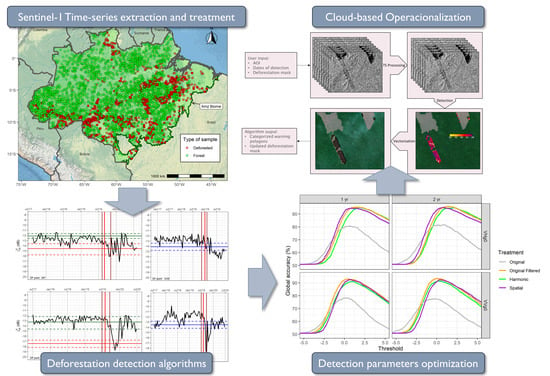
3. Materials and Methods

3.1. Materials

3.1.1. SAR Data

The data used in this research correspond to the Sentinel-1A (S1A) IW GRD dataset, made available by the European Space Agency (ESA) and pre-processed in the Google Earth Engine (GEE) platform [91]. The main characteristics of the input images are presented in Table 3.
The pre-processing procedure includes the following steps [92]:
  • Orbit file correction: Updates orbit metadata with a restituted orbit file.
  • GRD border noise removal: Removes low-intensity noise and invalid data on scene edges.
  • Thermal noise removal: Removes additive noise in sub-swaths to help reduce discontinuities between sub-swaths for scenes in multi-swath acquisition modes.
  • Radiometric calibration: Computes backscatter intensity using sensor calibration parameters in the GRD metadata.
  • Terrain correction (orthorectification): Converts data from ground range geometry, which does not take terrain into account, to normalized backscatter coefficient using the SRTM 30 m DEM.
Our area of interest (AOI) covers the entire Amazon biome within the Brazilian borders. The S1A data collection over the AOI stabilized between October and November 2016. Thus, the time interval that can be potentially used ranges between November 2016 and December 2019, totaling about 3 years of continuous acquisition, and approximately 30 yr−1 samples per location.
Most of the AOI can be considered as being flat or, at most, hilly, with few mountainous areas. A simple approach to angle correction was applied, where the original backscattering was corrected following the expression [93]:
γ 0 = σ 0 cos θ i
where σ 0 represents the normalized backscatter coefficient, θ i the local incidence angle (LIA), and γ 0 , known as gamma naught, is the backscattering coefficient normalized by the incidence angle. LIA was obtained using the procedure discussed in [94]. Mountainous areas should follow a more complex procedure, such as the one recently proposed in [95].

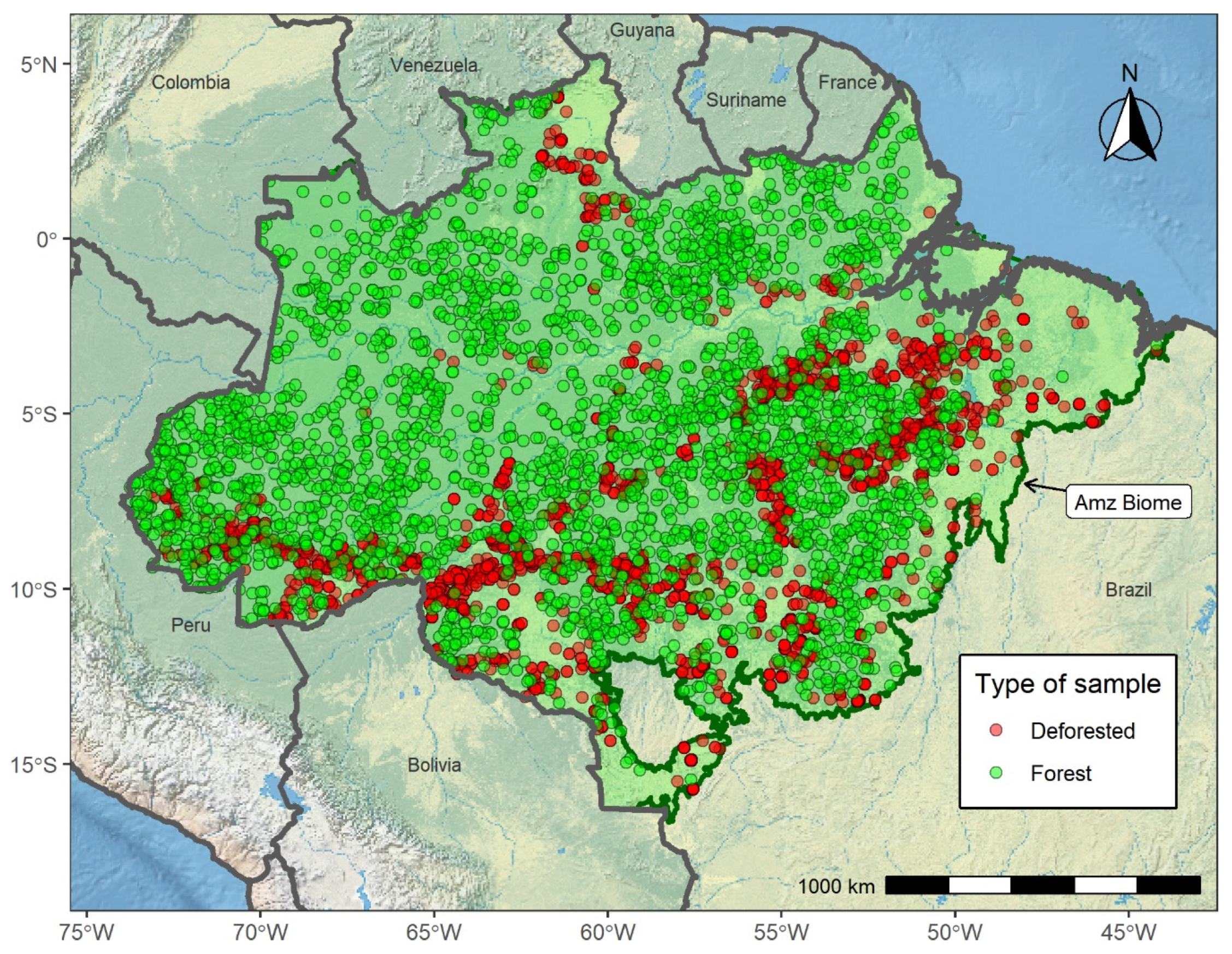
3.1.2. Sampling Spaces
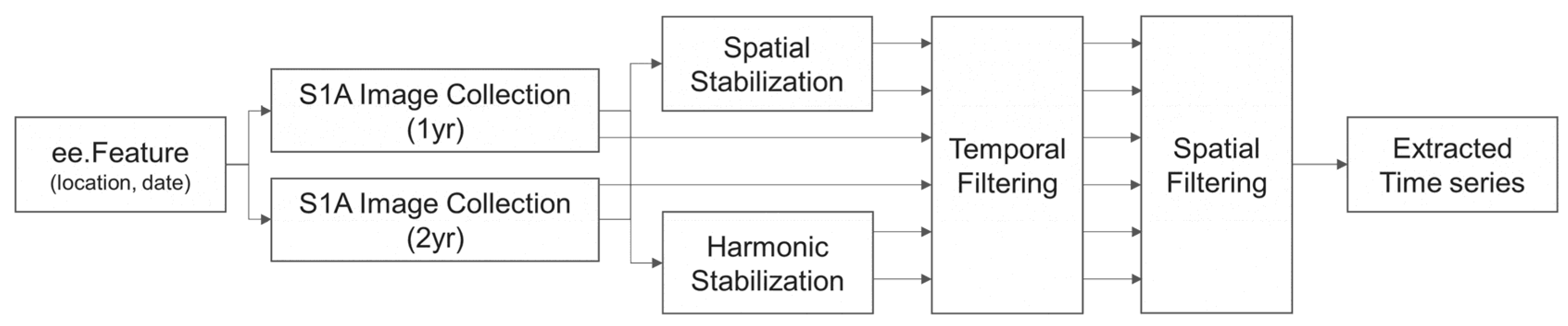
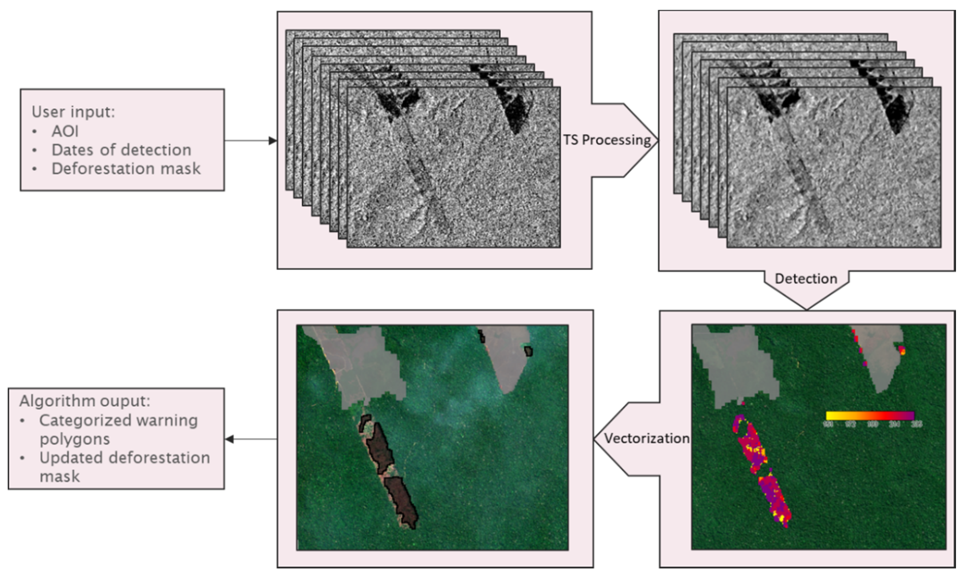
To test the proposed stabilization and detection techniques, we randomly sampled Sentinel-1A measurements in two different, basin-wide sampling spaces. The first sampling space corresponds to invariant forest regions. To define these areas with emerged, preserved primary forests, we excluded the forest areas affected by clear-cut deforestation and/or degradation from the Amazonian Biome region, as per the INPE up-to-date data available in the Terrabrasilis [96] website (http://terrabrasilis.dpi.inpe.br/). The resulting areas were then eroded using a 5000 m buffer to retain forest kernel areas. Finally, we retained all the pixels that had an NDVI median value higher than 0.85 during 2019, as measured in cloud-free observation of the Landsat-8 OLI sensor. As a result of those operations, performed using a GEE script, a total area of 18,630 Mha was delimited as the invariant forest sample region. The second sampling space corresponds to the deforested area sampling region—i.e., areas that have suffered a deforestation event. To define this space, we used the Mapbiomas Alerta confirmed and refined 2019 warning polygons (MBA2019). The MBA2019 collection (http://alerta.mapbiomas.org/) is the result of a sophisticated semi-automated processing chain that uses very high resolution daily optical images to confirm and refine warning polygons issued from different alert systems. Every MBA2019 warning polygon has two attributes, “before_dt” and an “after_dt”, which gives the date of the last cloud-free optical image before the deforestation and the first cloud-free optical image after the deforestation. An example of a selected MBA2019 polygon is shown in Figure 1. For this research, we built a subset from the MBA2019 collection, retaining the polygons issued from the DETER EWS system [97] larger than 1 ha, which had a validation time (lapse between the “before deforestation” and “after deforestation” optical image) lower than 4 months and a 3-month median NDVI greater than 0.82 before deforestation and lower than 0.69 after deforestation, as measured in a cloud-free observation of Landsat-8 OLI sensor. This selection is intended to avoid the effects of vegetation regrowth on the S1 signal. After selecting, a total of 2658 polygons were retained for analysis, encompassing all the Brazilian Amazon regions.
After defining the sampling spaces, a simple operation performed using the stratified sample routine of the GEE API allowed us to randomly sample 3000 locations in the invariant sample space and 3000 locations in the deforested area sample space. These locations are shown in Figure 2.

3.2. Methods

The extraction and processing sequence followed for every sample location is illustrated in Figure 3. To handle the number of images and processing needed to extract, filter, and stabilize in a time-effective fashion, we used the cloud-computing processing platform Google Earth Engine (GEE), which allowed us to perform a complex global analysis of remote sensing data using a simple programming interface. In this case, we used the GEE Python API.
To avoid the effect of the incidence angle in mountainous areas, we removed the observations that had local observation angles of more than 45° or less than 30°.

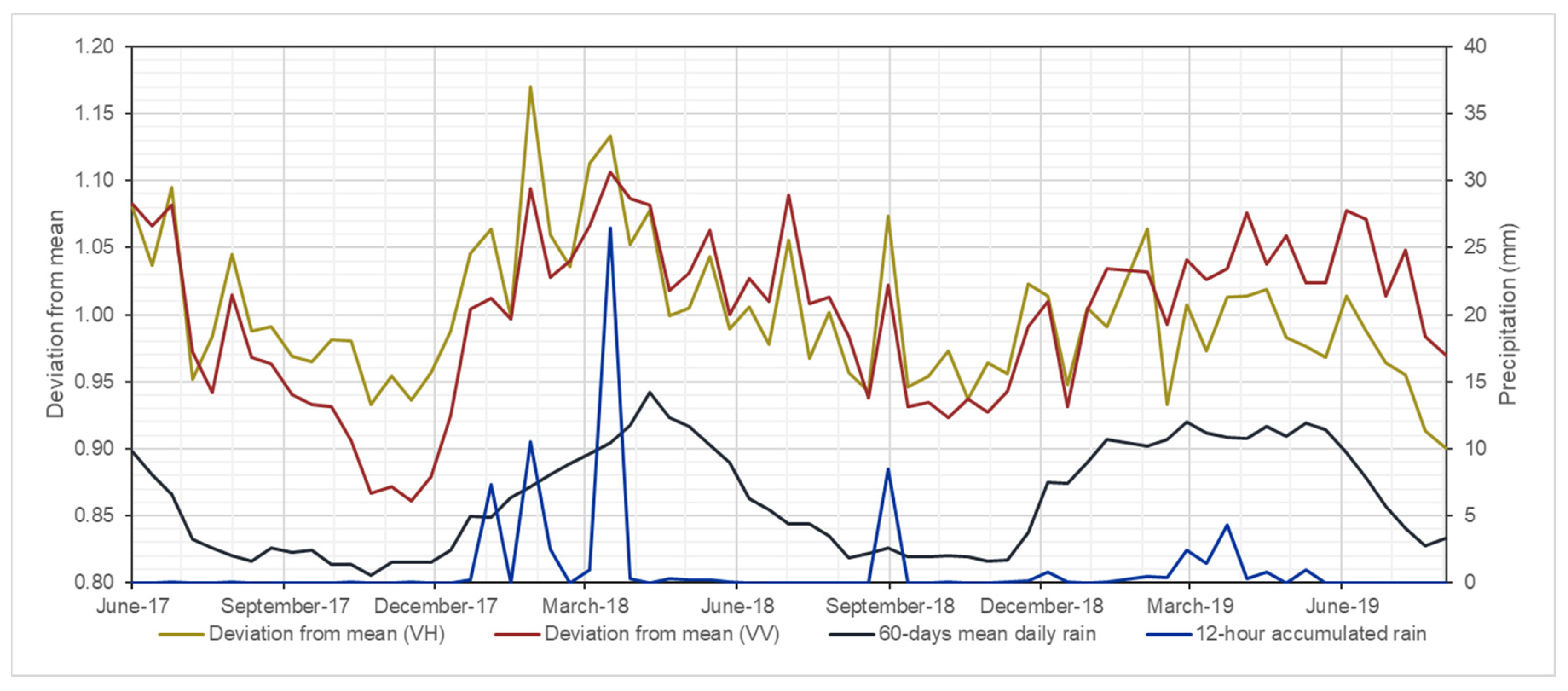
3.2.1. Time Series Stabilization

To stabilize SAR data time series, we used two different methods: First, we applied a simple pixel-wise no-trend harmonic fitting approach, like the one used in [28]. Additionally, we extended the spatial normalization technique used in [29] by improving its applicability to an operational environment. This proposed stabilization algorithm is built upon the premise that the variations of C-band backscattering over tropical dense forest areas are mainly due to variations in canopy moisture content, variations in the amount of intercepted rain, the occurrence of storm cells and variations in sensor calibration [26]. These variations can be slow pathed (alternation between dry and wet season) or quite fast (intense rain shower during the acquisition of the image data). Spatially, the variations have a global (calibration), regional (overall wetness of the canopy), or local (rain interception after a heavy shower) scale. Figure 4 shows an example of backscatter signal instabilities observed over an unaltered stretch of evergreen forest in Eastern Amazonia. In this example, one can see how the moisture content in the canopy directly influences the backscatter intensity in the long-term, following dry and wet season cycles, and in the short-term, due to heavy showers before the data acquisition.
In this regard, we may correct the variations of the SAR signal by computing a correction coefficient (CC) for every pixel of every image of a lengthy SAR image collection, taking the overall variations of the forested neighborhood of the pixel as a reference. Specifically, CC is computed as:
C C = F S ¯ T F S ¯ ¯  
where F S ¯ is the forest spatial mean of the pixel’s neighborhood, and T F S ¯ ¯ is the temporal mean of this same value, computed for every image of the time series.
”Forest spatial mean” denotes a spatial mean that solely considers the forest-covered areas of the pixel surroundings. The detailed steps in stabilization are as follows:
  • Masking of all the available images of the interest area, leaving only the forest pixels unmasked. The forest mask is computed from previous knowledge of the deforestation history of the area and then applied to all the sensor images of the interest area.
  • For every pixel of each image, the mean forest backscattering value is computed as the forest spatial mean of a 5 km radius neighborhood. This radius value was fixed considering the general spacing of the deforestation patches of the colonization roads of the Brazilian Amazon (the well-known ”fishbones”).
  • For every image, the correction coefficient is computed as the ratio between the forest spatial mean to the temporal mean of the same forest mean computed along the entire time series.
  • The final, stabilized backscatter value is computed by dividing the actual backscattering value by the correction coefficient.
This procedure allows the proposed stabilization to be applied to any area threatened by deforestation, with two caveats: (1) the user must have a reliable, up-to-date forest/non-forest map valid at the start of the detection period, and (2) the proposed procedure demands a great deal of computational resources. Its operational implementation should use a cloud-based solution, such as GEE.
To initially evaluate the effects of both stabilization algorithms, we computed the statistical parameters of the stabilized invariant forest time series and compared them with the original data. We used the standard deviation and coefficient of variation (CV) measures to perform this analysis. We then evaluated the stabilization algorithm using 1- and 2 year-long series.

3.2.2. Time Series Filtering

Speckle noise is a phenomenon common to all SAR measurement. In order to reduce speckle, we applied the spatio-temporal filtering procedure proposed in [98]. It has been applied with success over Sentinel-1A series [29,41,99], and it can be considered nowadays as a fundamental part of the processing chain of dense temporal SAR data. Following [21], the kth filtered image at position (x,y) is given by:
J k ( x , y ) = I k ( x , y ) N     i = 1 N I i ( x , y ) I i ( x , y ) ,   1 k N
where I k ( x , y ) is the backscattering value of image k at the position x,y and I k ( x , y ) is the speckle-free estimated value of the image k at the position x,y.
Additionally, a spatial filter was applied to every temporally-filtered image, as recommended by [98]. Previous works [100] point to the Refined Lee filter as a good compromise between noise-removal performance, edge preservation, and operational usability, reaching a performance similar to advanced filters based on complex computations. Thus, the filtering step is composed by the Quegan and Yu temporal filtering with a 5 × 5 box-car internal filter and 7 × 7 Refined Lee as the spatial filter.

3.2.3. Deforestation Detection

After stabilization and filtering, two different deforestation detection techniques were used, corresponding to the two main approaches to deforestation detection: Maximum Likelihood Classification and Adaptive Thresholding.
The pixel-wise maximum likelihood classification (MLC) approach used a Bayesian classification framework to classify S1 samples as belonging to forest or deforested areas. This approach has been successfully applied over SAR time series [69], and is based on the classic Bayesian conditional probability equation. Applied to our context, it is expressed by the following equation:
P ( ω i | x t ) = p ( x t | ω i ) P ( ω i ) 1 n p ( x t | ω j ) P ( ω j )    
where P ( ω i | x t ) is the posterior probability of the sample x t belong to the state ω i , P ( ω i ) is the prior probability of the state ω i , and p ( x t | ω i ) is the likelihood of x t given the state ω i .
The simplest Bayesian classification framework then builds a discriminant function g i ( x t ) = P ( ω i | x t ) for every possible state and then classify the state of x t based on the discriminant with the maximum value. Other monotonic discriminant functions can be used. Following [101], we used:
g i ( x t ) = ln P ( ω i | x t )
In our case, we consider only two possible states: forest (F) and deforested (DF). Following (4) we can define a two-class discriminant function (called a dichotomizer) as:
g ( x t ) = g D F ( x t ) g F ( x t ) = ln P ( ω D F | x t ) ln P ( ω F | x t )
Substituting (4) in (6), we obtain the final expression of our discriminator:
g ( x t ) = ln p ( x t | D F ) p ( x t | F ) ln P ( D F ) P ( F )
where p ( x t | D F ) is the likelihood of x f being deforested, given by the pdf of the deforestation state; p ( x t | F ) the likelihood of x f being forest, given by the probability density function (pdf) of the forest state; P ( D F ) the prior probability of the deforestation state; and P ( F ) the prior probability of the forest state.
Finally, we classify x t as being a deforested location if g ( x t ) > 0 .
As the ln P(DF)/P(F) constant (that we call the detection threshold) is initially unknown (although we know that generally, P(F) is much greater than P(DF)), we used the value that maximizes the accuracy of the detection results, following a heuristic approach. In this manner, we ran all the detection algorithms using a range of thresholds going from 0 (deforested and forested equally probable) to 10 (forest much more probable). A value of 3, for instance, means that the a priori probability of finding a forest pixel is e 3   20 times higher than the probability of finding a pixel that was deforested during the detection period.
The maximum-likelihood classification of the F/DF time series requires the determination of the probability density function of the backscattering values, for the F and DF classes. While the determination of the parameters of the speckle-filtered forest series was trivial once we had a wealth of data points of invariant forest locations, the deforestation samples are somewhat trickier to study as we do not know exactly the time of the deforestation. Additionally, even if we know that backscattering values normally drop after a deforestation event, we do not know exactly the time that every deforested location would take to recover the previous backscattering values. Thus, to separate the forest and non-forest samples of the deforestation time series, we used a 2-component finite mixture statistical modeling technique [102], using a six-month sampling of the training TS, starting at some point after the deforestation event (this date is given by the after_dt parameter associated with every warning polygon), and assuming the normality of the subjacent distributions. Then, we studied the relationship between the modeled F and DF distribution parameters, looking for a simple and meaningful relationship that might be applied to other locations where the time or occurrence of deforestation is unknown.
The statistical model to be applied to the F/DF classis during the maximum-likelihood is defined by studying the statistical distribution of the extracted time series. We used the Shapiro–Wilk and Kolmogorov–Smirnoff tests to determine the statistical distribution models more suitable for the forest-invariant extracted samples, before and after the stabilization and filtering processes. This characterization was made on a pixel-wise basis, taking all the available samples at the forest locations, building the corresponding γ0 time series (TS) and determining the Shapiro–Wilk and Kolmogorov–Smirnoff test p-values for normal and gamma distributions, respectively. We assumed the deforested samples to follow a similar statistical distribution model.
The second, more straight-forward detection approach uses an adaptive linear threshold (ALT) based on the relationship between the mean and the minimum value of the forest TS. The premise of this method is that the SAR signal variability over tropical forest tends to be constant, and thus, any sample that falls below an interval of backscattering values should be considered as being non-forest and flagged as a deforested sample. Following this premise, the forest threshold is defined as:
T h F = 1 n i [   γ F 0 ¯ i min ( γ F 0 ) i ]    
where n is the number of collected forest locations, γ F 0 ¯ i is the mean value of the forest TS of the ith location, and min ( γ F 0 ) i is the minimum value of the forest TS of the ith location.
Following (8), we defined the forest threshold T h F using (a) a set of training samples, extracted from the invariant forest locations, and (b) a set of training samples extracted from the deforested locations samples predating the deforestation event (soon-to-be deforested series). Then, all the TS were thresholded using the computed T h F value for both cases. In order to optimize the detection performance, we tested the detection performance of a set of thresholds around the T h F value.

3.2.4. Detection Validation

As the final purpose of the proposed SAR data processing techniques to improve near real-time deforestation detection at the pixel-level, we applied a validation framework based on the statistical evaluation of the detection results at randomly sampled 20-m sized pixels. We decided to operate at the 20-m pixel, as this is the resolution of the original S1A images in range-azimuth geometry after multi-looking.
Once defined, the sampling spaces for invariant forest and deforested classes, and the images processed following the steps detailed until here, we proceeded to extract data series at random locations using the GEE python API.
For every random location, we extracted the time series corresponding to:
  • Original backscattering values;
  • Stabilized values;
  • Filtered values.
Both VH and VV polarizations were used and evaluated during this phase. We also used two different time TS-lengths: 1 and 2 years. For every sampled location, we performed a complete detection processing using the two methods described above, looking for deforestation that occurred in a 4-month interval after the ”after deforestation” date, in the case of the deforested locations, and after a random date, in the case of the unaltered forest locations. If deforestation is detected, the day of the first deforestation warning will be recorded, and the sample will be classified as ”deforested”. If no deforestation is detected, the sample will be classified as ”no deforested”. This procedure will be repeated for every sample, using different detection thresholds.
Once the detection process was completed, we computed the confusion matrix for every combination of Polarization, Treatment, and Threshold. The confusion matrix elements were combined to compute global accuracy (ACC), Specificity (TNR), and Sensitivity (TPR). They are given by:
A c c u r a c y   ( A C C ) = T P + T N T P + F P + T N + F N
S p e c i f i t y   ( T N R ) = T N T N + F P
S e n s i t i v i t y   ( T P R )   = T P T P + F N
where:
  • TP = True Positives, or the number of deforested locations classified as deforested;
  • TN = True Negatives, or the number of forested locations classified as non-deforested;
  • FP = False Positives, or the number of forested locations classified as deforested;
  • FN = False Negatives, or the number of deforested locations classified as non-deforested
The Specificity, also called Selectivity or true negative rate (TNR), is the most important parameter to consider in an EWS, as it measures the ability of the algorithm to avoid false warnings (commission errors). The Sensitivity, also called Recall or true positive rate (TPR), complements the Specificity by informing the completeness of the algorithm detection (the lack of omission errors). The accuracy parameter is used as a measure of the global performance of the algorithms, but we use it with precaution, as it tends to give the same weight to omissions and commission errors, being our operational context much more sensitive to commission errors. Therefore, the different methods and treatments proposed here were compared using Accuracy, but also their relationship between Specificity and Sensitivity, by using Receiver–Operator Characteristic (ROC) curves and by comparing the TPR value for a given, optimal, TNR.

3.3. Code Availability

The above-described acquisition, processing, and validation of the Sentinel-1 data were performed in three different environments:
  • Earth Engine Javascript Code Editor: Definition of the sampling locations.
  • Earth Engine Python API: Extraction of filtered and stabilized time series at the selected locations.
  • R [103]: Analysis of the results.
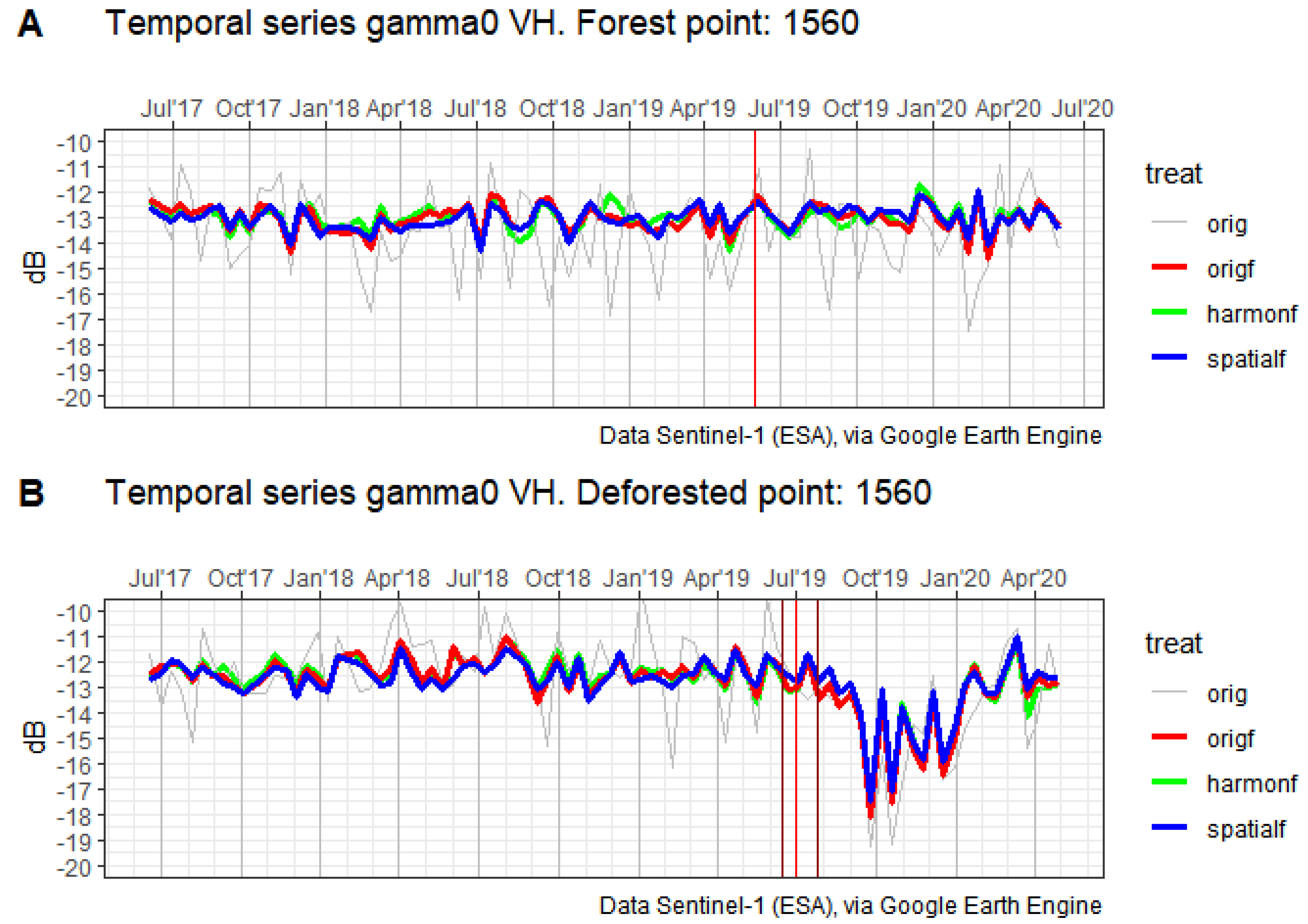
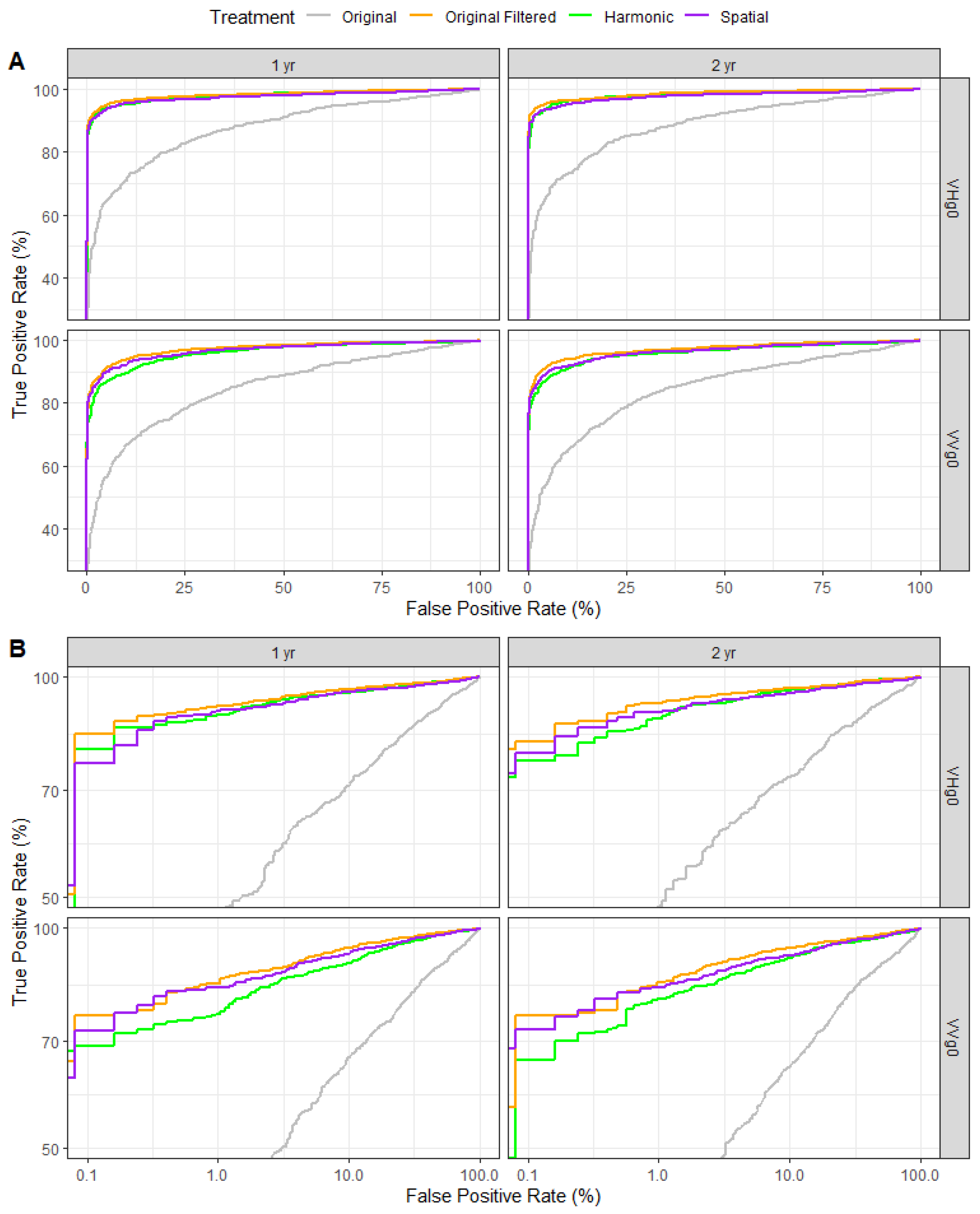
All the used scripts and the resulting data are available in https://github.com/jdoblas/DETER_SAR_RS.

4. Results

Following the proposed methodology, we extracted 24 different time-series of incidence angle-corrected intensity S1A backscattering (which we name as γ 0 ), in every one of the 6000 randomly selected locations. The number of series per location corresponds to the combinations of two different collecting periods (1 and 2 years) in two different polarizations (VH and VV), undergoing 6 different types of treatment, labeled as follows:
  • orig—original Sentinel-1 backscattering samples.
  • origf—original TS filtered.
  • harmon—original TS stabilized using harmonic fitting.
  • harmonf—original TS stabilized using harmonic fitting and then filtered.
  • spatial—original TS stabilized using spatial stabilization.
  • spatialf—original TS stabilized using spatial stabilization and then filtered
Figure 5 shows two examples of each set of time series.
As some of the randomly selected locations did not have an adequate Sentinel-1A covering, the initial extracting procedures resulted in 2978 deforested locations and 2983 invariant forest locations with complete (n ≥ 20) TS, rather than the expected 3000 locations for every class. The missing locations are located near the Brazilian southern border, where some marginal regions are being collected by the Sentinel-1B satellite, without any covering of the Sentinel-1A. At the initial stages of this research, we observed a substantial difference in the backscattering patterns of the satellites, and thus we decided to focus the remainder of this work on the S1A measurements.
After the Local Incidence Angle filtering procedure, we retained 2565 deforested locations and 2480 invariant forest locations, which represents 86.13% and 83.13% of the original deforested and forested points, respectively. The total number of collected SAR measurements is 8,726,898, divided into different polarizations, data collecting period, and treatments.
The main characteristics of the times series are summarized in Tables S1 and S2 (Supplementary Materials), for the forest and deforested locations, and for every treatment and polarization.
The mean value of the forest γ0 was determined as being −12.4 and −6.25 dB for VH and VV polarizations, respectively. The unfiltered series have a substantive variability in both polarizations of ~1.75 dB (1σ), which is reduced to ~0.57 dB when applied to the proposed speckle filtering.
The mean backscattering values of the deforested series are consistently lower than the forest series, reaching −13.1 and −7.6 dB for VH and VV polarizations.
Regarding stabilization results, all the tested stability measures showed a statistically significant difference between the non-stabilized series and the stabilized ones. The stabilized TS show a diminution of the variability, as measured by the CV, of 3%–5% (for harmonic stabilization) and ~10% for the spatial stabilization (Table S3 and Figure S1, Supplementary Materials). Other measures of variation, such as mean absolute deviation (MAD), standard deviation (SD), and interquantile ratio (IQR) yielded very similar results.
Before enterprise pixel-wise modeling, we tested the forest time-series for normality. The results of the normality Shapiro–Wilk testing showed that ~80% of the filtered TS are normal (p = 0.05) (see Figure S2 and Table S4, Supplementary Materials). The non-filtered series were successfully fitted using a Gamma distribution (see Table S5, Supplementary Materials).

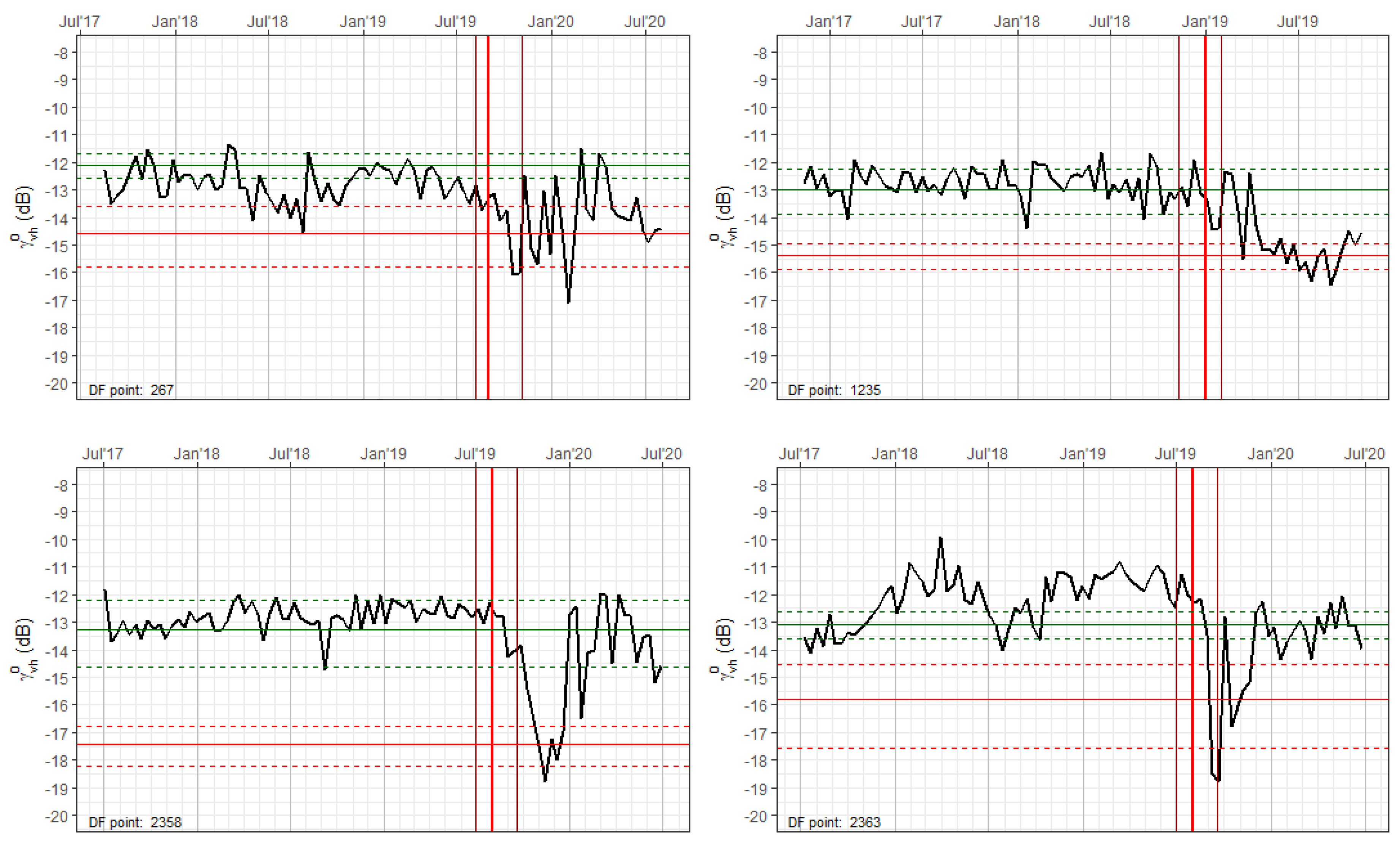
4.1. Detection of Deforestation

As detailed previously, the deforestation detection procedure followed two different approaches. The first approach, based on maximum-likelihood classification, uses the deforestation TS to build a 2-component mixture model of normal distributions, which should represent the statistical properties of the forested (F) and deforested (DF) samples (Figure 6).
To verify the separability of the obtained distributions, we computed the Jeffries–Matsushita (JM) distance [104] between the F and DF components, for every TS. All treatments presented a good separability with mean JM distances greater than 1.19 (see Figure S3, Supplementary Materials).
After deducing the parameters of the statistical distribution of the F/DF series in a set of training samples, we studied the relationship between them. As can be seen in Figure 7, the means of the deforested class have a good linear relationship with the means of the forest class, with R² values ranging from 0.59 to 0.64.
Meanwhile, the variance values of the deforested distributions did not correlate with the values of the variance, or the mean, of the forested samples, with R² values below 0.2. Thus, we used the mean value of the variance in every treatment to characterize deforestation variance.
Thus, the statistical distribution of the deforested class was modeled, in every location, as a normal distribution with a mean linearly related to the (known) mean of the forest class, and a constant variance, which was deducted from the training dataset.
Once we established the statistical parameters of the F/DF distributions, we were ready to start the maximum-likelihood detection process using the maximum likelihood approach. Initially, we computed the values of p(F) and p(DF) of every sample of the validation dataset during a four-month detection period. Then, the likelihood of the sample belonging to the deforested class was computed by dividing p(DF) by p(F) (Figure S4, Supplementary Materials).
The final results of the detection procedure using the Maximum Likelihood approach are represented in Table 4, Figure 8 and Figure 9.
We also considered the best results given an optimum level of TNR. Based on field experience, we fixed this level as 99.5%, which is equivalent to a rate of false positives of 0.5%. Table 5 shows the results of the MLC detection procedure given this level of TNR.
The second deforestation detection technique used—i.e., Adaptive linear thresholding (ALT)—is based on the study of the variability of the values of the forest time series. For every forest TS, we computed the difference between its mean and its p1 (1% percentile) value. We also computed this relationship for the deforested values, selecting the samples measured before the deforestation event (as specified by the corresponding warning polygon metadata) in a 50%-split training subset.
The results of this analysis show that the distance between the forest mean and the minimum value of the forest TS is nearly constant (see Figure 10). Similarly, we may use this finding as a straight-forward approach to detect deforestation by using a range of values around the distance to threshold and flagging deforestation-suspected values of the time-series (see how this can be applied to some TS in Figure 11).
After learning with the training dataset about the relationship between the forests’ backscattering means and minima, we applied this relationship to the validation dataset, flagging as deforested the samples that fell below the expected minimum, following a simple procedure to find the optimum thresholding level:
  • Forest_mean = mean value of the validation TS samples before the deforestation date.
  • Treatment_distance_mean = mean of the distances between the mean and the p1 value of the training dataset TS, for every treatment.
  • Treatment_distance_sd = standard deviation of the distances between the mean and the p1 value of the training dataset TS, for every treatment.
  • Central threshold = Forest_mean-Treatment_distance_mean.
  • For thresholding_factor = −5 to 5:
    • Threshold = Central_threshold-(Treatment_distance_sd*thresholding_factor).
    • Flag TS samples < Threshold.
We ran this procedure for all the training datasets’ TS and computed the TS that were correctly flagged and those that were not. Then, we computed the confusion matrix and accuracy measures (see Table 6, Figure 12 and Figure 13).
We also considered the best results of the ALT method given an optimum level of TNR. Based on field experience, we fixed this level as 99.5%, which is equivalent to a rate of false positives of 0.5% (Table 7).
The results of the validation phase showed that both methods yielded satisfactory results. However, the ALT method performed better than the MLC method, especially regarding the TPR measure of accuracy in a fixed false alarm rate context. This index reached 89.61% using ALT methodology, overcoming MLC’s best result (78.92%).

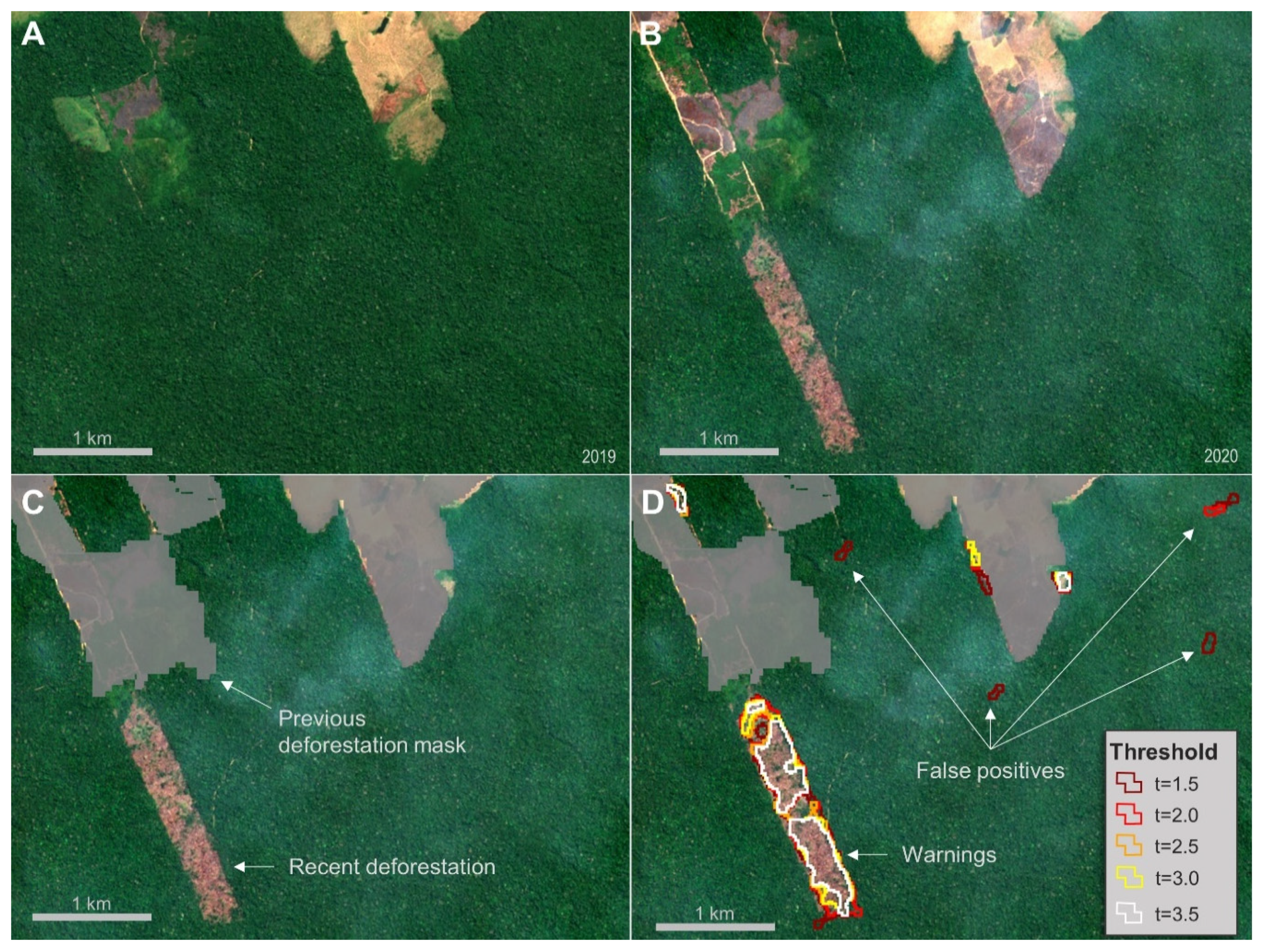
4.2. Algorithm Scalation to Support an EWS
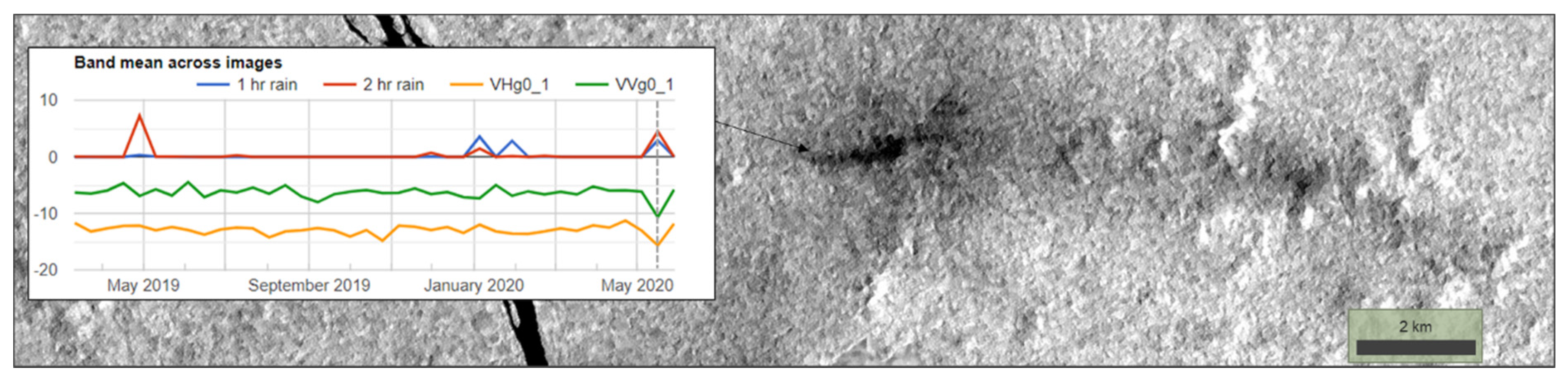
The preliminary results of the location-based algorithms led us to a further step, where we developed a set of algorithms to apply the proposed methodologies to arbitrary areas using the google earth engine (GEE) platform. Thus, we built a three-step procedure to create warning polygons associated with the backscattering anomalies, as detected by the ALT and MLC methods, in user-defined areas. The steps taken were: (1) processing of the image collections available for the area and period specified by the user (including a 2-year training period); (2) a pixel-based detection routine, which produces a multi-band image with the detection thresholding; and (3) vectorization of the warning raster to create a set of warning polygons.
This operational implementation is detailed in Figure 14.
A fully-operational, completely automated EWS based on the proposed methodologies was coded in the GEE Python API in the context of INPE’s DETER project. The so-called DETERSAR system has been up and running since 21 June 2020, and it has already issued 25,107 warning alerts over five critical areas in the Brazilian Amazon Basin (as of 22 September 2020).
During the development of the EWS version of the algorithms proposed here, we were forced to reevaluate the algorithm’s parametrization to fit the needs of the final users of the EWS. In this case, the user of the system will be willing to sacrifice accuracy in exchange for a very low false-positive rate (FPR). As a matter of fact, a false deforestation warning might misguide ground enforcement teams, and provoke an unnecessary waste of time and resources. This low-FPR aspect linked to the EWS is emphasized by [105].
To illustrate this point, we consider the case of the ALT method proposed here, in which the global accuracy optimum threshold (1.5) produces several false positives, linked to its FPR (1.9%). Even if this number is very low, a EWS user might want to choose a stricter threshold, in order to avoid those false positives. Visual inspection (Figure 15) suggests a threshold value of 2.5. By shifting the threshold in this way, we lost global accuracy—from 95.9% to 94.4%—but we lowered the FPR from 1.9% to 0.5%, which dramatically reduced the number of false warnings of a potential SAR-based EWS system.

5. Discussion

Initially, the vast number of time series collected for the present work allowed the examination of the sign of backscattering change related to deforestation events. The mean backscattering values of the deforested series are consistently lower than the forest ones, reaching −13.1 and −7.6 dB for VH and VV polarizations, respectively, against −12.4 and −6.25 dB for invariant forest areas. Thus, we can conclude that deforestation causes a decrease in C-band SAR backscattering. Meanwhile, a closer look at the extracted time series shows a more complex reality. The typical temporal profile of a clear-cut area in the Amazon tropical forest found during this work encompasses different stages, which we can tentatively summarize as:
  • Forest canopy with little or no damage.
  • Initial deforestation, where some tree trunks and standing trees remain.
  • Fire removes vegetation and promotes double bounce (remaining standing trees with bare soil) returns to the sensor.
  • Pasture grows with increasing precipitation and remnants of burned vegetation
  • Pasture reaches a decimetric height and becomes hardly distinguishable from the original forest cover for SAR-C incoherent signal.
Up to the submission of this article, no research has been published focusing on those short-term patterns, but based the patterns of the extracted time series, we consider that clear-cut deforestation will cause a ~6-month cycle of low backscattering in the C-SAR measurements as a working hypothesis. The length of this period will depend on a variety of factors, such as the type of deforestation, the season of the year, and the use of the deforested area.
Regarding variability, the extracted series variability ( σ 1.75   dB in both polarizations) is highly consistent with the models proposed by Benninga et al. [26], which predict a radiometric uncertainty of 2.02 dB for a 20 × 20 m measurement of VH and 1.77 dB for VV backscattering measures.
The results of the stabilization procedures indicate that the stabilized series are more stable than the original ones, the spatial stabilization being more performant than the harmonic stabilization.
The detection algorithm results, though very satisfactory, did not register substantial differences between the un-stabilized series and the stabilized ones. It is true that spatial stabilization offers the best results in MLC workflow, but the difference in accuracy (94.36% to 93.93%) was not as prominent as expected. The advantages of spatial stabilization are more evident when using higher thresholds, such as those used in operational EWS. In this case, the differences in accuracy of the MLC method can improve from 84.16% to 89.05% using spatial stabilization.
Visual inspection of the stabilized time series (available on the online repository) reveals that some of the contrast and spikes related to deforestation are reduced by the stabilization processes. This is especially true for the dry season, where the forest canopy reduces its moisture content, and thus its backscattering intensity. Stabilization algorithms then tend to raise values of the TS, diminishing the contrast of eventual deforestation events. Our work proves that the loss of accuracy linked to this effect can overcome the benefits of stabilization.
These results can be seen as complementary to those presented by Reiche et al. [28] which first applied harmonic fitting to stabilize SAR TS in Bolivian dry forests, which are known to have a strong seasonality. Our results show that this correction may be unnecessary for evergreen forests. We still think that stabilization can be of great value in transitional forests, such as those of the Amazonia-Cerrado ecotone.
False deforestation alerts due to high-density storm clouds, relatively frequent in the change-of-season months, are still a problem to be resolved. Several anomalies linked to this phenomenon were detected in time series while verifying false-alerts events, and in actual SAR images (Figure 16). This kind of anomalies can disrupt the operation of a fully-automated EWS, as they can create vast deforestation polygons in untouched forest areas. Future attempts to control and stabilize SAR measurements should rely on high-resolution meteorological measurements [27]. Until then, confirmation of alerts should be mandatory in a SAR-based EWS.
As an overall analysis of the detection results, it can be said that the obtained global accuracy and the false positive and negative rates were high, given the relative simplicity of the proposed methods and the continental extension of the experiment. An EWS user interested in reducing the false positive rate (FPR) to a minimum (e.g., 0.5%) will still have a true positive rate higher than 79%, in the case of the MLC method, and 90%, in the case of the ALT method. That means that using these principles we can build a very reliable EWS system with a low rate of omissions. The duration of the training period seems to improve the ALT method results. A 3-year period should slightly improve these results.
Another key aspect of the proposed TS-based pixel-wise detection methodologies is the ability to follow the dynamics of deforestation, as for every deforestation warning, it is possible to see the day of deforestation of every pixel (Figure 17).

6. Conclusions

In this work, we investigated the performance of two different stabilization methods using two different deforestation detection algorithms in an evergreen tropical forest context. The results indicate that spatial stabilization is useful and can improve detection results if used within a maximum-likelihood detection approach. Meanwhile, stabilization did not seem to improve the detection results while using an Adaptive Linear Thresholding approach.
Both deforestation detection methods offered good results, and its implementation as the base of an operation Early Warning System seems very promising, especially if combined with the use of thresholds that can spatially change as a function of the risk of deforestation.
The validation of our results used the DETER polygons refined by the MapBiomas Alerta initiative. These polygons constitute an extraordinary source of training and validating samples, and should be used in future developments, as the initiative continues to generate warnings polygons.
Global application of the proposed methodologies should be straightforward, by adapting the provided GEE scripts. The used mask layers, which are specific to the Brazilian Amazon, can be substituted by global datasets such as Hansen’s Global Forest Change data [106].
Further research should focus on the use of polarimetric and interferometric attributes of change detection, meteorological stabilization using high-resolution meteorological data, integration with other sensors, and detection in transitions to savanna regions.

Supplementary Materials

The following are available online at https://0-www-mdpi-com.brum.beds.ac.uk/2072-4292/12/23/3922/s1, Table S1: Characteristics of the collected forest Time Series, Table S2: Characteristics of the collected deforestation Time Series, Figure S1: Box-plot of the coefficient of variation of the forest speckle-filtered time series, Table S1: Mean reduction of the variability of the time series, Figure S2: Results of the Shapiro-Wilk normality test applied to the treated and non-treated forested TS, Table S4: Results of the Shapiro-Wilk test for normality of Forest time series, Table S5: Results of the Kolmogorov-Smirnoff test for gamma-distribution fitting of unfiltered Forest time series, Figure S3: Jeffries-Matsushita distance of the F/DF classes as computed by the finite mixture algorithm, Figure S4: Density distribution of the values of the deforestation log-likelihood of the validation samples.

Author Contributions

Conceptualization, methodology, programming, writing, J.D.; supervision, Y.S. and S.S.; writing—review and editing, Y.S., A.C., L.A., S.S., and C.A.; funding acquisition, C.A. All authors have read and agreed to the published version of the manuscript.

Funding

This research was funded by the National Council of Technological and Scientific Development—CNPq, grant number 444418/2018-0.

Acknowledgments

We are grateful to four anonymous reviewers for their feedback and suggestions that helped to improve the manuscript. The first author would like to thank Guido Lemoine (JRC) and Felix Greifeneder (EURAC) for their contributions to GEE coding.

Conflicts of Interest

The authors declare no conflict of interest.

References

  1. We Lost a Football Pitch of Primary Rainforest Every 6 Seconds in 2019. Available online: https://blog.globalforestwatch.org/data-and-research/global-tree-cover-loss-data-2019 (accessed on 30 June 2020).
  2. Monitoramento do Desmatamento da Floresta Amazônica Brasileira por Satélite. Available online: http://www.obt.inpe.br/OBT/assuntos/programas/amazonia/prodes (accessed on 10 July 2020).
  3. Early Warning Systems for Deforestation: An Explainer. Available online: https://blog.globalforestwatch.org/data-and-research/early-warning-systems-for-deforestation-an-explainer (accessed on 27 September 2019).
  4. Soares-Filho, B.; Moutinho, P.; Nepstad, D.; Anderson, A.; Rodrigues, H.; Garcia, R.; Dietzsch, L.; Merry, F.; Bowman, M.; Hissa, L.; et al. Role of Brazilian Amazon protected areas in climate change mitigation. Proc. Natl. Acad. Sci. USA 2010, 107, 10821–10826. [Google Scholar] [CrossRef] [PubMed] [Green Version]
  5. Assunção, J.; Gandour, C.; Rocha, R. DETERring Deforestation in the Brazilian Amazon: Environmental Monitoring and Law Enforcement TL-May. Clim. Policy Initiat. Rep. 2013, 1–36. Available online: https://climatepolicyinitiative.org/wp-content/uploads/2013/05/DETERring-Deforestation-in-the-Brazilian-Amazon-Environmental-Monitoring-and-Law-Enforcement-Technical-Paper.pdf (accessed on 30 October 2019).
  6. Nepstad, D.; McGrath, D.; Stickler, C.; Alencar, A.; Azevedo, A.; Swette, B.; Bezerra, T.; DiGiano, M.; Shimada, J.; Da Motta, R.S.; et al. Slowing Amazon deforestation through public policy and interventions in beef and soy supply chains. Science 2014, 344, 1118–1123. [Google Scholar] [CrossRef] [PubMed]
  7. Finer, B.M.; Novoa, S.; Weisse, M.J.; Petersen, R.; Mascaro, J.; Souto, T.; Stearns, F.; Martinez, R.G. Combating deforestation: From satellite to intervention. Science 2018, 360, 1303–1305. [Google Scholar] [CrossRef] [PubMed]
  8. Indonesian Ban on Clearing New Swaths of Forest to be Made Permanent. Available online: https://news.mongabay.com/2019/06/indonesian-ban-on-clearing-new-swaths-of-forest-to-be-made-permanent (accessed on 20 June 2020).
  9. Hansen, M.C.; Krylov, A.; Tyukavina, A.; Potapov, P.V.; Turubanova, S.; Zutta, B.; Ifo, S.; Margono, B.; Stolle, F.; Moore, R. Humid tropical forest disturbance alerts using Landsat data. Environ. Res. Lett. 2016, 11, 034008. [Google Scholar] [CrossRef]
  10. Reiche, J.; Lucas, R.; Mitchell, A.L.; Verbesselt, J.; Hoekman, D.H.; Haarpaintner, J.; Kellndorfer, J.M.; Rosenqvist, A.; Lehmann, E.A.; Woodcock, C.E.; et al. Combining satellite data for better tropical forest monitoring. Nat. Clim. Chang. 2016, 6, 120–122. [Google Scholar] [CrossRef]
  11. Argenti, F.; Lapini, A.; Alparone, L.; Bianchi, T. A tutorial on speckle reduction in synthetic aperture radar images. IEEE Geosci. Remote Sens. Mag. 2013, 1, 6–35. [Google Scholar] [CrossRef] [Green Version]
  12. Davies, K.; Smith, E.K. Ionospheric effects on satellite land mobile systems. IEEE Antennas Propag. Mag. 2002, 44, 24–31. [Google Scholar] [CrossRef]
  13. Bouvet, A.; Le Toan, T.; Floury, N.; MacKlin, T. An end-to-end error model for classification methods based on temporal change or polarization ratio of SAR intensities. IEEE Trans. Geosci. Remote Sens. 2010, 48, 3521–3538. [Google Scholar] [CrossRef]
  14. Atlas, D.; Rosenfeld, D.; Wolff, D.B. C-band attenuation by tropical rainfall in Darwin, Australia, using climatologically tuned Ze-R relations. J. Appl. Meteorol. 1993, 32, 426–430. [Google Scholar] [CrossRef] [Green Version]
  15. Kasilingam, D.; Lin, I.I.; Lim, H.; Khoo, V.; Alpers, W.; Lim, T.K. Investigation of tropical rain cells with ERS SAR imagery and ground-based weather radar. In Proceedings of the Third ERS Symposium on Space at the Service of our Environment, Florence, Italy, 14–21 March 1997; Guyenne, T.D., Danesy, D., Eds.; European Space Agency, ESA Publications Division: Noordwijk, The Netherlands, 1997; Volume 414, pp. 1603–1608. [Google Scholar]
  16. Lin, I.I.; Kasilingam, D.; Alpers, W.; Lim, T.K.; Lim, H.; Khoo, V. A quantitative study of tropical rain cells from ERS SAR imagery. In Proceedings of the International Geoscience and Remote Sensing Symposium, Singapore, 3–8 August 1997; Stein, T.I., Ed.; Institute of Electrical and Electronics Engineers: New York, NY, USA, 1997; pp. 1527–1529. [Google Scholar]
  17. Dobson, M.C.; Pierce, L.; McDonald, K.; Sharik, T. Seasonal change in radar backscatter from mixed conifer and hardwood forests in northern Michigan. Dig.-Int. Geosci. Remote Sens. Symp. 1991, 3, 1121–1124. [Google Scholar] [CrossRef]
  18. Henderson, F.M.; Lewis, A.J. Principles and Applications of Imaging Radar, Manual of Remote Sensing, 3rd ed.; John Wiley and Sons, Inc.: Somerset, NJ, USA, 1999; Volume 2. [Google Scholar]
  19. De Jong, J.; Klaassen, W.; Ballast, A. Rain storage in forests detected with ERS tandem mission SAR. Remote Sens. Environ. 2000, 72, 170–180. [Google Scholar] [CrossRef] [Green Version]
  20. Cisneros Vaca, C.; Van Der Tol, C. Sensitivity of sentinel-1 to rain stored in temperate forest. In Proceedings of the International Geoscience and Remote Sensing Symposium (IGARSS), Valencia, Spain, 22–27 July 2018; IGARSS: Valencia, Spain, 2018; pp. 5330–5333. [Google Scholar]
  21. Quegan, S.; Toan, L.; T, Y.; J, J.; Ribbes, F.; Floury, N. Multitemporal ERS SAR analysis applied to forest mapping. Remote Sens. Environ. 2000, 38, 741–753. [Google Scholar] [CrossRef]
  22. Danklmayer, A.; Doring, B.R.J.; Schwerdt, M.; Chandra, M. Assessment of atmospheric propagation effects in SAR images. IEEE Trans. Geosci. Remote Sens. 2009, 47, 3507–3518. [Google Scholar] [CrossRef]
  23. Moore, R.K.; Mogili, A.; Fang, Y.; Beh, B.; Ahamad, A. Rain measurement with SIR-C/X-SAR. Remote Sens. Environ. 1997, 59, 280–293. [Google Scholar] [CrossRef]
  24. Koyama, C.N.; Watanabe, M.; Hayashi, M.; Shimada, M. The effect of precipitation and soil moisture variations on (partial) polarimetric L-band SAR backscatter in tropical forest regions. In Proceedings of the International Geoscience and Remote Sensing Symposium, Singapore, 3–8 August 2017; Institute of Electrical and Electronics Engineers: New York, NY, USA, 2017; pp. 2450–2453. [Google Scholar]
  25. El Hajj, M.; Baghdadi, N.; Zribi, M.; Bazzi, H. Synergic use of Sentinel-1 and Sentinel-2 images for operational soil moisture mapping at high spatial resolution over agricultural areas. Remote Sens. 2017, 9, 1292. [Google Scholar] [CrossRef] [Green Version]
  26. Benninga, H.-J.F.; van der Velde, R.; Su, Z. Impacts of Radiometric Uncertainty and Weather-Related Surface Conditions on Soil Moisture Retrievals with Sentinel-1. Remote Sens. 2019, 11, 2025. [Google Scholar] [CrossRef] [Green Version]
  27. Doblas, J.; Carneiro, A.; Shimabukuro, Y.; Sant’Anna, S.; Aragão, L. Assessment of rainfall influence on sentinel-1 time series on amazonian tropical forests aiming deforestation detection improvement. In Proceedings of the IEEE Latin American GRSS ISPRS Remote Sensing Conference (LAGIRS), Santiago de Chile, Chile, 22–27 March 2020; IEEE: Santiago de Chile, Chile, 2020; pp. 397–402. [Google Scholar]
  28. Reiche, J.; Verhoeven, R.; Verbesselt, J.; Hamunyela, E.; Wielaard, N.; Herold, M. Characterizing tropical forest cover loss using dense Sentinel-1 data and active fire alerts. Remote Sens. 2018, 10, 777. [Google Scholar] [CrossRef] [Green Version]
  29. Reiche, J.; Hamunyela, E.; Verbesselt, J.; Hoekman, D.; Herold, M. Improving near-real time deforestation monitoring in tropical dry forests by combining dense Sentinel-1 time series with Landsat and ALOS-2 PALSAR-2. Remote Sens. Environ. 2017, 204, 147–161. [Google Scholar] [CrossRef]
  30. El Hajj, M.; Baghdadi, N.; Zribi, M.; Angelliaume, S. Analysis of Sentinel-1 radiometric stability and quality for land surface applications. Remote Sens. 2016, 8, 406. [Google Scholar] [CrossRef] [Green Version]
  31. Doblas, J.; Carneiro, A.; Shimabukuro, Y.; Sant’anna, S.; Aragão, L.; Pereira, F.R.S. Stabilization of sentinel-1 sar time-series using climate and forest structure data for early tropical deforestation detection. ISPRS Ann. Photogramm. Remote Sens. Spat. Inf. Sci. 2020, 5, 89–96. [Google Scholar] [CrossRef]
  32. FAO. Global Forest Resources Assessment 2020-Key Findings; Food and Agriculture Organization of the United nations: Rome, Italy, 2020. [Google Scholar] [CrossRef]
  33. FAO. Global Forest Resources Assessment 2020: Terms and Definition; Food and Agriculture Organization of the United nations: Rome, Italy, 2020. [Google Scholar]
  34. INPE. Metodologia Utilizada nos Projetos PRODES e DETER; INPE: São José dos Campos, Brazil, 2019. [Google Scholar]
  35. Almeida-Filho, R.; Rosenqvist, A.; Shimabukuro, Y.E.; Dos Santos, J.R. Evaluation and perspectives of using multitemporal L-band SAR data to monitor deforestation in the Brazilian Amazônia. IEEE Geosci. Remote Sens. Lett. 2005, 2, 409–412. [Google Scholar] [CrossRef]
  36. Shimabukuro, Y.E.; Almeida-Filho, R.; Kuplich, T.M.; de Freitas, R.M. Quantifying optical and SAR image relationships for tropical landscape features in the Amazônia. Int. J. Remote Sens. 2007, 28, 3831–3840. [Google Scholar] [CrossRef]
  37. Whittle, M.; Quegan, S.; Uryu, Y.; Stüewe, M.; Yulianto, K. Detection of tropical deforestation using ALOS-PALSAR: A Sumatran case study. Remote Sens. Environ. 2012, 124, 83–98. [Google Scholar] [CrossRef]
  38. Watanabe, M.; Koyama, C.; Hayashi, M.; Kaneko, Y.; Shimada, M. Development of early-stage deforestation detection algorithm (advanced) with PALSAR-2/ScanSAR for JICA-JAXA program (JJ-FAST). Int. Geosci. Remote Sens. Symp. 2017, 2017, 2446–2449. [Google Scholar] [CrossRef]
  39. Tanase, M.A.; Villard, L.; Pitar, D.; Apostol, B.; Petrila, M.; Chivulescu, S.; Leca, S.; Borlaf-Mena, I.; Pascu, I.S.; Dobre, A.C.; et al. Synthetic aperture radar sensitivity to forest changes: A simulations-based study for the Romanian forests. Sci. Total Environ. 2019, 689, 1104–1114. [Google Scholar] [CrossRef] [PubMed]
  40. Joshi, N.; Mitchard, E.T.A.; Woo, N.; Torres, J.; Moll-Rocek, J.; Ehammer, A.; Collins, M.; Jepsen, M.R.; Fensholt, R. Mapping dynamics of deforestation and forest degradation in tropical forests using radar satellite data. Environ. Res. Lett. 2015, 10, 034014. [Google Scholar] [CrossRef] [Green Version]
  41. Bouvet, A.; Mermoz, S.; Ballère, M.; Koleck, T.; Le Toan, T. Use of the SAR Shadowing Effect for Deforestation Detection with Sentinel-1 Time Series. Remote Sens. 2018, 10, 1250. [Google Scholar] [CrossRef] [Green Version]
  42. Rahman, M.M.; Sumantyo, J.T.S. Mapping tropical forest cover and deforestation using synthetic aperture radar (SAR) images. Appl. Geomatics 2010, 2, 113–121. [Google Scholar] [CrossRef] [Green Version]
  43. Balzter, H.; Cole, B.; Thiel, C.; Schmullius, C. Mapping CORINE land cover from Sentinel-1A SAR and SRTM digital elevation model data using random forests. Remote Sens. 2015, 7, 14876–14898. [Google Scholar] [CrossRef] [Green Version]
  44. Pereira, L.O.; Freitas, C.C.; Sant’Anna, S.J.S.; Reis, M.S. ALOS/PALSAR Data Evaluation for Land Use and Land Cover Mapping in the Amazon Region. IEEE J. Sel. Top. Appl. Earth Obs. Remote Sens. 2016, 9, 5413–5423. [Google Scholar] [CrossRef]
  45. Angelis, C.F.; Freitas, C.C.; Valeriano, D.M.; Dutra, L.V. Multitemporal analysis of land use/land cover JERS-1 backscatter in the Brazilian tropical rainforest. Int. J. Remote Sens. 2002, 23, 1231–1240. [Google Scholar] [CrossRef]
  46. Saatchi, S.S.; Soares, J.V.; Alves, D.S. Mapping deforestation and land use in Amazon rainforest by using SIR-C imagery. Remote Sens. Environ. 1997, 59, 191–202. [Google Scholar] [CrossRef]
  47. Mercier, A.; Betbeder, J.; Rumiano, F.; Baudry, J.; Gond, V.; Blanc, L.; Bourgoin, C.; Cornu, G.; Ciudad, C.; Marchamalo, M.; et al. Evaluation of Sentinel-1 and 2 Time Series for Land Cover Classification of Forest–Agriculture Mosaics in Temperate and Tropical Landscapes. Remote Sens. 2019, 11, 979. [Google Scholar] [CrossRef] [Green Version]
  48. Cassol, H.L.G.; Shimabukuro, Y.E.; Beuchle, R.; Aragão, L.E.O.C. Sentinel-1 Time-Series Analysis For Detection Of Forest Degradation By Selective Logging. In Proceedings of the Simpósio Brasileiro de Sensoriamento Remoto; INPE: Santos, SP, Brazil, 2019; pp. 755–758. [Google Scholar]
  49. Varghese, A.O.; Suryavanshi, A.; Joshi, A.K. Analysis of different polarimetric target decomposition methods in forest density classification using C band SAR data. Int. J. Remote Sens. 2016, 37, 694–709. [Google Scholar] [CrossRef]
  50. Yamaguchi, Y.; Moriyama, T.; Ishido, M.; Yamada, H. Four-Component Scattering Model for Polarimetric SAR Image Decomposition based on Asymmetric Covariance Matrix. IEEE Trans. Geosci. Remote Sens. 2005, 104, 1699–1706. [Google Scholar] [CrossRef]
  51. Cloude, S.R.; Pottier, E. A review of target decomposition theorems in radar polarimetry. IEEE Trans. Geosci. Remote Sens. 1996, 34, 498–518. [Google Scholar] [CrossRef]
  52. Wiederkehr, N.C.; Gama, F.F.; Santos, J.R.; Mura, J.C.; Bispo, P.C.; Liesenberg, V. Análise de imagens polarimétricas do sensor ALOS/PALSAR-2 para discriminação do uso e cobertura da terra em região de influência da Floresta Nacional do Tapajós. In Proceedings of the XXVII Congr. Bras. Cartogr., Rio de Janeiro, Brazil, 6–9 November 2017; SBC: Rio de Janeiro, Brazil, 2017; pp. 654–658. [Google Scholar]
  53. Gama, F.F.; Paradella, W.R.; Mura, J.C.; Santos, A.R. dos Técnicas de interferometria radar na detecção de deformação superficial utilizando dados orbitais. In Proceedings of the Anais XVI Simposio Brasileiro de Sensoriamento Remoto-SBSR, Foz do Iguaçu, Brazil, 13–18 April 2013; INPE: Foz de Iguaçu, Brazil, 2013; pp. 6917–6922. [Google Scholar]
  54. Hagberg, J.O.; Ulander, L.M.H.; Askne, J. Repeat-pass SAR interferometry over forested terrain. IEEE Trans. Geosci. Remote Sens. 1995, 33, 331–340. [Google Scholar] [CrossRef]
  55. Askne, J.I.H.; Dammert, P.B.G.; Ulander, L.M.H.; Smith, G. C-band repeat-pass interferometric SAR observations of the forest. IEEE Trans. Geosci. Remote Sens. 1997, 35, 25–35. [Google Scholar] [CrossRef]
  56. Luckman, A.; Baker, J.; Wegmuller, U. Repeat-pass interferometric coherence measurements of tropical forest from JERS and ERS satellites. In Proceedings of the IGARSS ’98. Sensing and Managing the Environment. 1998 IEEE International Geoscience and Remote Sensing. Symposium Proceedings: (Cat. No.98CH36174), Seattle, WA, USA, 6–10 July 1998; Volume 4, pp. 1828–1830. [Google Scholar]
  57. Strozzi, T.; Wegmuller, U.; Luckman, A.; Balzter, H. Mapping deforestation in Amazon with ERS SAR interferometry. Int. Geosci. Remote Sens. Symp. 1999, 2, 767–769. [Google Scholar] [CrossRef]
  58. Luckman, A.; Baker, J.; Wegmüller, U. Repeat-pass interferometric coherence measurements of disturbed tropical forest from JERS and ERS satellites. Remote Sens. Environ. 2000, 73, 350–360. [Google Scholar] [CrossRef]
  59. Gaboardi, C. Utilização de Imagem de Coerência SAR Para Classificação Do Uso Da Terra: Floresta Nacional Do Tapajós. Ph.D. Thesis, Instituto Nacional de Pesquisas Espaciais (INPE), Sao Jose dos Campos, Brazil, 11 June 2002. [Google Scholar]
  60. Hamadi, A.; Villard, L.; Borderies, P.; Albinet, C.; Koleck, T.; Le Toan, T. Comparative Analysis of Temporal Decorrelation at P-Band and Low L-Band Frequencies Using a Tower-Based Scatterometer over a Tropical Forest. IEEE Geosci. Remote Sens. Lett. 2017, 14, 1918–1922. [Google Scholar] [CrossRef]
  61. El Idrissi Essebtey, S.; Villard, L.; Borderies, P.; Koleck, T.; Monvoisin, J.P.; Burban, B.; Le Toan, T. Temporal Decorrelation of Tropical Dense Forest at C-Band: First Insights From the TropiScat-2 Experiment. IEEE Geosci. Remote Sens. Lett. 2019, 1–5. [Google Scholar] [CrossRef]
  62. Diniz, J.M. Avaliação do Potencial Dos Dados Polarimétricos Sentinel-1A Para Mapeamento Do Uso e Cobertura da Terra na Região de Ariquemes (RO). Master’s Thesis, Instituto Nacional de Pesquisas Espaciais (INPE), Sao Jose dos Campos, Brazil, 15 February 2019. [Google Scholar]
  63. Sica, F.; Pulella, A.; Nannini, M.; Pinheiro, M.; Rizzoli, P. Repeat-pass SAR interferometry for land cover classification: A methodology using Sentinel-1 Short-Time-Series. Remote Sens. Environ. 2019, 232, 111277. [Google Scholar] [CrossRef]
  64. Cihlar, J.; Pultz, T.J.; Gray, A.L. Change detection with synthetic aperture radar. Int. J. Remote Sens. 1992, 13, 401–414. [Google Scholar] [CrossRef]
  65. Dempster, A.P.; Laird, D.; Rubin, D.B. Maximum Likelihood from Incomplete Data via the EM Algorithm. J. R. Stat. Soc. Ser. B 1977, 39, 1–38. [Google Scholar]
  66. Bruzzone, L.; Prieto, D.F. Automatic Analysis of the Difference Image for Unsupervised Change Detection. IEEE Trans. Geosci. Remote Sens. 2000, 38, 1171–1182. [Google Scholar] [CrossRef] [Green Version]
  67. Kittler, J.; Illingworth, J. Minimum Error Thresholding. Pattern Recognit. 1986, 19, 41–47. [Google Scholar] [CrossRef]
  68. Bazi, Y.; Bruzzone, L.; Melgani, F. An Unsupervised Approach Based on the Generalized Gaussian Model to Automatic Change Detection in Multitemporal SAR Images. IEEE Trans. Geosci. Remote Sens. 2005, 43, 874–887. [Google Scholar] [CrossRef] [Green Version]
  69. Reiche, J.; de Bruin, S.; Hoekman, D.; Verbesselt, J.; Herold, M. A Bayesian approach to combine landsat and ALOS PALSAR time series for near real-time deforestation detection. Remote Sens. 2015, 7, 4973–4996. [Google Scholar] [CrossRef] [Green Version]
  70. Frontiers in Forest Monitoring: Research Horizons for Global Forest Watch. Available online: https://www.youtube.com/watch?v=aM227q31uZ8 (accessed on 15 August 2020).
  71. Pirrone, D.; Bovolo, F.; Bruzzone, L. A Novel Framework Based on Polarimetric Change Vectors for Unsupervised Multiclass Change Detection in Dual-Pol Intensity SAR Images. IEEE Trans. Geosci. Remote Sens. 2020, 1–16. [Google Scholar] [CrossRef]
  72. Conradsen, K.; Nielsen, A.; Schou, J.; Skriver, H. A test statistic in the complex wishart distribution and its application to change detection in polarimetric SAR data. IEEE Trans. Geosci. Remote Sens. 2003, 41, 4–19. [Google Scholar] [CrossRef] [Green Version]
  73. Yang, W.; Yang, X.; Yan, T.; Song, H.; Xia, G.S. Region-Based Change Detection for Polarimetric SAR Images Using Wishart Mixture Models. IEEE Trans. Geosci. Remote Sens. 2016, 54, 6746–6756. [Google Scholar] [CrossRef]
  74. Conradsen, K.; Nielsen, A.A.; Skriver, H. Determining the Points of Change in Time Series of Polarimetric SAR Data. IEEE Trans. Geosci. Remote Sens. 2016, 54, 3007–3024. [Google Scholar] [CrossRef] [Green Version]
  75. Muro, J.; Canty, M.; Conradsen, K.; Hüttich, C.; Nielsen, A.A.; Skriver, H.; Remy, F.; Strauch, A.; Thonfeld, F.; Menz, G. Short-term change detection in wetlands using Sentinel-1 time series. Remote Sens. 2016, 8, 795. [Google Scholar] [CrossRef] [Green Version]
  76. Cloude, S.R. The Dual Polarisation Entropy / Alpha Decomposition. In Proceedings of the 3rd International Workshop on Science and Applications of SAR Polarimetry and Polarimetric Interferometry, Frascati, Italy, 22–26 January 2007; pp. 1–6. [Google Scholar]
  77. Ji, K.; Wu, Y. Scattering mechanism extraction by a modified Cloude-Pottier decomposition for dual polarization SAR. Remote Sens. 2015, 7, 7447–7470. [Google Scholar] [CrossRef] [Green Version]
  78. Khati, U.; Kumar, V.; Bandyopadhyay, D.; Musthafa, M.; Singh, G. Identification of forest cutting in managed forest of Haldwani, India using ALOS-2/PALSAR-2 SAR data. J. Environ. Manag. 2018, 213, 503–512. [Google Scholar] [CrossRef]
  79. Lavalle, M. A new automated algorithm for detecting forest disturbances with the dual-polarimetric SAR alpha angle. Int. Geosci. Remote Sens. Symp. 2017, 2017, 5299–5302. [Google Scholar] [CrossRef]
  80. Wahl, D.E.; Yocky, D.A.; Jakowatz, C.V.; Simonson, K.M. A New Maximum-Likelihood Change Estimator for Two-Pass SAR Coherent Change Detection. IEEE Trans. Geosci. Remote Sens. 2016, 54, 2460–2469. [Google Scholar] [CrossRef]
  81. Rizzoli, P.; Bello, J.L.B.; Pulella, A.; Sica, F.; Zink, M. A Novel Approach to Monitor Deforestation in the Amazon Rainforest by Means of Sentinel-1 and Tandem-X Data. In Proceedings of the 2018 IEEE International Geoscience and Remote Sensing Symposium, {IGARSS} 2018, Valencia, Spain, 22–27 July 2018; pp. 192–195. [Google Scholar]
  82. White, R.G. Change detection in SAR imagery. Int. J. Remote Sens. 1991, 12, 339–360. [Google Scholar] [CrossRef]
  83. Zhu, X.X.; Tuia, D.; Mou, L.; Xia, G.-S.; Zhang, L.; Xu, F.; Fraundorfer, F. Deep Learning in Remote Sensing. IEEE Geosci. Remote Sens. Mag. 2017, 5, 8–36. [Google Scholar] [CrossRef] [Green Version]
  84. Gong, M.; Zhao, J.; Liu, J.; Miao, Q.; Jiao, L. Change Detection in Synthetic Aperture Radar Images Based on Deep Neural Networks. IEEE Trans. Neural Netw. Learn. Syst. 2016, 27, 125–138. [Google Scholar] [CrossRef]
  85. Gong, M.; Yang, H.; Zhang, P. Feature learning and change feature classification based on deep learning for ternary change detection in SAR images. ISPRS J. Photogramm. Remote Sens. 2017, 129, 212–225. [Google Scholar] [CrossRef]
  86. Liu, J.; Gong, M.; Qin, K.; Zhang, P. A Deep Convolutional Coupling Network for Change Detection Based on Heterogeneous Optical and Radar Images. IEEE Trans. Neural Netw. Learn. Syst. 2018, 29, 545–559. [Google Scholar] [CrossRef] [PubMed]
  87. Lv, N.; Chen, C.; Qiu, T.; Sangaiah, A.K. Deep Learning and Superpixel Feature Extraction Based on Contractive Autoencoder for Change Detection in SAR Images. IEEE Trans. Ind. Inform. 2018, 14, 5530–5538. [Google Scholar] [CrossRef]
  88. Chen, H.; Jiao, L.; Liang, M.; Liu, F.; Yang, S.; Hou, B. Fast unsupervised deep fusion network for change detection of multitemporal SAR images. Neurocomputing 2019, 332, 56–70. [Google Scholar] [CrossRef]
  89. Xu, S.; Mu, X.; Chai, D.; Zhang, X. Remote sensing image scene classification based on generative adversarial networks. Remote Sens. Lett. 2018, 9, 617–626. [Google Scholar] [CrossRef]
  90. Zhu, X.X.; Montazeri, S.; Ali, M.; Hua, Y.; Wang, Y.; Mou, L.; Shi, Y.; Xu, F.; Bamler, R. (In Press.) Deep Learning Meets SAR. Available online: https://arxiv.org/pdf/2006.10027.pdf (accessed on 1 September 2020).
  91. Gorelick, N.; Hancher, M.; Dixon, M.; Ilyushchenko, S.; Thau, D.; Moore, R. Google Earth Engine: Planetary-scale geospatial analysis for everyone. Remote Sens. Environ. 2017, 202, 18–27. [Google Scholar] [CrossRef]
  92. Sentinel-1 Algorithms. Available online: https://developers.google.com/earth-engine/guides/sentinel1 (accessed on 10 July 2020).
  93. Woodhouse, I.H. Introduction to Microwave Remote Sensing; CRC Press: Boca Raton, FL, USA, 2006; ISBN 0-415-27123-1. [Google Scholar]
  94. About Sentinel-1 Radiometric Terrain Correction in Preprocessing. Available online: https://groups.google.com/g/google-earth-engine-developers/c/3-q0TEwa-Tk (accessed on 10 July 2019).
  95. Vollrath, A.; Mullissa, A.; Reiche, J. Angular-based radiometric slope correction for Sentinel-1 on google earth engine. Remote Sens. 2020, 12, 1867. [Google Scholar] [CrossRef]
  96. Assis, L.F.F.G.; Ferreira, K.R.; Vinhas, L.; Maurano, L.; Almeida, C.; Carvalho, A.; Rodrigues, J.; Maciel, A.; Camargo, C. TerraBrasilis: A Spatial Data Analytics Infrastructure for Large-Scale Thematic Mapping. ISPRS Int. J. Geo-Inf. 2019, 8, 513. [Google Scholar] [CrossRef] [Green Version]
  97. Diniz, C.G.; de Almeida Souza, A.A.; Santos, D.C.; Dias, M.C.; da Luz, N.C.; de Moraes, D.R.; Maia, J.S.; Gomes, A.R.; da Silva Narvaes, I.; Valeriano, D.M.; et al. DETER-B: The New Amazon Near Real-Time Deforestation Detection System. IEEE J. Sel. Top. Appl. Earth Obs. Remote Sens. 2015, 8, 3619–3628. [Google Scholar] [CrossRef]
  98. Quegan, S.; Yu, J.J. Filtering of multichannel SAR images. IEEE Trans. Geosci. Remote Sens. 2001, 39, 2373–2379. [Google Scholar] [CrossRef]
  99. Carreiras, J.M.B.; Quegan, S.; Tansey, K.; Page, S. Sentinel-1 observation frequency significantly increases burnt area detectability in tropical SE Asia. Environ. Res. Lett. 2020. [Google Scholar] [CrossRef]
  100. Cozzolino, D.; Verdoliva, L.; Scarpa, G.; Poggi, G. Nonlocal CNN SAR image despeckling. Remote Sens. 2020, 12, 1006. [Google Scholar] [CrossRef] [Green Version]
  101. Duda, R.O.; Hart, P.E.; Stork, D.G. Pattern Classification; John Wiley & Sons: New York, NY, USA, 2001; ISBN 978-0-471-05669-0. [Google Scholar]
  102. Scrucca, L.; Fop, M.; Murphy, T.B.; Raftery, A.E. Mclust 5: Clustering, classification and density estimation using Gaussian finite mixture models. R J. 2016, 8, 289–317. [Google Scholar] [CrossRef] [PubMed] [Green Version]
  103. R Core Team. R: A Language and Environment for Statistical Computing; R Foundation for Statistical Computing: Vienna, Austria, 2020. [Google Scholar]
  104. Rees, G. The Remote Sensing Data Book; Cambridge University Press: Cambridge, UK, 1999; ISBN 052148040X. [Google Scholar]
  105. Weisse, M.J.; Noguerón, R.; Eduardo, R.; Vicencio, V.; Castillo Soto, D.A. Use of Near-Real-Time Deforestation Alerts: A Case Study from Peru; World Resources Institute: Washington, DC, USA, 2019. [Google Scholar]
  106. Hansen, M.C.; Potapov, P.V.; Moore, R.; Hancher, M.; Turubanova, S.A.; Tyukavina, A.; Thau, D.; Stehman, S.V.; Goetz, S.J.; Loveland, T.R.; et al. High-Resolution Global Maps of 21st-Century Forest Cover Change. Science 2013, 342, 850–853. [Google Scholar] [CrossRef] [PubMed] [Green Version]
Figure 1. Example of a selected MapBiomas Alerta warning polygon selected for deforestation signal characterization. The id of the displayed polygon is 6561, and it is located in the Novo Progresso municipality, Pará state (Brazil).
Remotesensing 12 03922 g001
Figure 2. Map of the sampling locations used during this research.
Remotesensing 12 03922 g002
Figure 3. Pixel-wise time series extraction and processing sequence. All the steps were executed using the Google Earth Engine Python API.
Remotesensing 12 03922 g003
Figure 4. Example of the relationship between the deviation of the backscatter signal from the three-year average and the short-term (12-h) and long-term (60 days) accumulated precipitation at the time of the image acquisition. Mean backscattering data extracted from Sentinel-1 IW-GRD images over a 5-km square of invariant forest patch in Portel (Brazil). Rainfall data computed from IMERG data.
Remotesensing 12 03922 g004
Figure 5. Example of extracted (A) forest and (B) deforested time series. Only VH two-year collections are showed. The red thin vertical lines represent the location reported before and after dates of deforestation. The red bold line represents the reported date of deforestation.
Remotesensing 12 03922 g005
Figure 6. Results of the finite mixture model algorithm in four different deforested locations in the Amazon basin. The time series are speckle-filtered non-stabilized VH backscattering. The continuous and dashed horizontal lines represent the mean and the 2σ interval of the two modeled components, assumed to represent forest (green) and deforested classes (red). The red thin vertical lines represent the location reported before and after dates of deforestation. The red bold line represents the reported date of deforestation.
Remotesensing 12 03922 g006
Figure 7. Correlation between the forest and deforested means for VH (A) and VV polarizations (B).
Remotesensing 12 03922 g007
Figure 8. Global accuracy of the maximum likelihood detection procedure.
Remotesensing 12 03922 g008
Figure 9. Receiver–Operator Characteristic (ROC) curves associated with the maximum likelihood detection procedure. (A) ”Classical” chart in linear scale; (B) detailed view using a logarithmic scale. The vertical red line indicates the optimal TNR level (1%) for an Early Warning System (EWS).
Remotesensing 12 03922 g009
Figure 10. Relationship between the mean value of the forest VH backscattering and the minimum (p1) value of the time series in forest pixels (A). As an alternative analysis, chart (B) shows the relationship between the mean and the difference between the mean and the p1 value.
Remotesensing 12 03922 g010
Figure 11. Speckle-filtered original VH time series of four deforested locations in the Amazon. The blue line represents the adaptive threshold automatically computed based on the regional relationship between backscattering means and minima. The dashed lines represent the 2σ interval of the global threshold distribution. The red thin vertical lines represent the location reported before and after dates of deforestation. The red bold line represents the reported date of deforestation.
Remotesensing 12 03922 g011
Figure 12. Global accuracy of the adaptive linear thresholding detection procedure.
Remotesensing 12 03922 g012
Figure 13. ROC curves associated to the adaptive linear thresholding detection procedure. (A) Using a linear scale. (B) Log-scaled detail.
Remotesensing 12 03922 g013
Figure 14. Proposed operationalization of the reviewed methods.
Remotesensing 12 03922 g014
Figure 15. ALT detection results in a deforested area in Apuí municipality, Amazonas state (Brazil). (A): Optical image before deforestation. (B): Optical image after deforestation. (C): Previous deforestation mask showed in grey. (D): Detected deforestation polygons. The application of the global accuracy optimal threshold (1.5) creates some false deforestations alerts, corresponding to the FPR associated with the threshold. More rigorous thresholds avoid false positives while maintaining a reasonable rate of true positives. In this case, the selected threshold would be around 2.5. Background images: Sentinel-2 10-m resolution mosaics. The GEE scripts used to produce this figure are available at the project repository.
Remotesensing 12 03922 g015
Figure 16. Anomalies in Sentinel-1 backscattering measurements due to heavy rainstorms can produce false deforestation alerts. In the figure, a deforestation warning, measuring 359 ha. was related to a heavy-rain episode registered by Global Precipitation Measurement (GPM) records (left panel, the vertical dashed line shows the date of the image). Other peaks in rain profiles did not provoke anomalies. This is due to the difference in the resolution of the SAR data (20 m) and the GPM data (~5 km).
Remotesensing 12 03922 g016
Figure 17. Time-series based detection can be used to track the dynamics of deforestation. In the figure, the progression of deforestation in a cleared patch in Apuí (Amazonas State, Brazil), from the primer clearings (yellow) to the last ones (purple).
Remotesensing 12 03922 g017
Table 1. Summary of the most important sources of errors and ambiguity in Synthetic Aperture Radar (SAR) measurements over forested surfaces found in the literature.
EffectBandRef
XCLP
Faraday Rotation- --+++[12]
Raincells+++
(−2 to −2.4 dB@80 mm/hr)
--[22,23]
Rain interception+
+ 2 to +3 dB
-
+1 to +1.5 dB
-
+1 to +2 dB
- -[17,24]
Soil moistureNR-
0.11–0.5 dB/[vol%] (VV)
0.08–0.01 dB/[vol%] (VH)
+
+1 dB (HH) +2 dB (HV)
NR[24,25]
”- -”: negligible; “-“: little importance; ”+”: require correction or masking before normal use; ”++”: compromise the use of data; ”NR”: non-reviewed.
Table 2. Selected references for backscattering change after tropical forest clear-cut.
BandPolarizationBackscattering ChangeReferenceForest Type and Location
CVH−2.0 dB[28]Tropical forest with dry season (Riau, Indonesia)
VV−2.0 dB[41]
−2.57 dB[29]Dry tropical forest (Santa Cruz, Bolivia)
LHH+1.2 dB[38]Early deforestation stage, tropical rainforest (Uyacali, Peru)
−5.0 dB[36]Completed deforestation, tropical rainforest w/dry season (Rondônia, Brazil)
−1.0 to −2.0 dB[42]Tropical rainforest (Bangladesh)
HV−11.0 dB[29]Dry tropical forest (Santa Cruz, Bolivia)
−2.3 to −3.0 dB[40]Tropical rainforest (Madre de Dios, Peru)
−6.0 dB[42]Tropical rainforest (Bangladesh)
−1.2 dB[38]Completed deforestation, tropical rainforest (Uyacali, Peru)
Table 3. Main characteristics of the SAR data during the study.
CharacteristicValue
Observation satelliteSentinel-1A (S1A)
SAR bandC-band (5.405 GHz, 5.625 cm)
Acquisition modeInterferometric Wide Swath (IW)
Orbit modeDescending
Image productGRD, high resolution
Multilooking4 × 1
Spatial resolution10 m *
Revisit time12 days
*: Nominal resolution. The real resolution of the multi-looked image is 20 (azimuth) × 22 m (range).
Table 4. Final results of the maximum likelihood classification (MLC) detection (only 10 best results in terms of global accuracy showed). DF = Number of deforested TS, F = Number of forest TS, TP = True positives, FP = False positives FP = False positives, TNR = True Negative Rate, TPR = True Positive Rate, ACC = Global Accuracy.
PeriodPol.TreatmentThreshold FactorDFFTPFPACC (%)TNR (%)TPR (%)
2 yrVHg0spatialf2.361280123911864894.3696.1392.66
1 yrVHg0spatialf2.741281123911734394.0196.5391.57
2 yrVHg0origf2.821280123911926593.9394.7593.12
1 yrVHg0origf2.581281123912058093.8193.5494.07
1 yrVHg0origf2.561281123912068193.8193.4694.15
2 yrVHg0harmonf3.281280123911978893.2192.993.52
1 yrVHg0harmonf3.3212811239119411192.1491.0493.21
1 yrVHg0harmonf3.2612811239119811592.1490.7293.52
1 yrVHg0harmonf3.2412811239119911692.1490.6493.60
2 yrVVg0origf2.081280123911597792.1493.7990.55
Table 5. Final results of the MLC detection with a fixed TNR~99.5% (0.5% of false positives), ordered by TPR. Only the 10 top results shown. DF = Number of deforested TS; F = Number of forest TS; TP = True positives; FP = False positives; TNR = True Negative Rate; TPR = True Positive Rate; ACC = Global Accuracy.
PeriodPol.TreatmentThreshold FactorDFFTPFPACC (%)TNR (%)TPR (%)
1 yrVHg0spatialf4.36128112391011689.0599.5278.92
2 yrVHg0spatialf4.5612801239986688.0999.5277.03
2 yrVHg0origf5.0612801239887684.1699.5269.3
2 yrVVg0spatialf4.212801239847682.5799.5266.17
2 yrVVg0spatialf4.1812801239847682.5799.5266.17
2 yrVHg0harmonf6.3612801239751778.7299.4458.67
2 yrVVg0origf4.0212801239750678.7299.5258.59
1 yrVHg0origf5.8412811239747678.5799.5258.31
1 yrVVg0spatialf4.9612811239724677.6699.5256.52
1 yrVHg0harmonf7.2212811239667675.499.5252.07
Table 6. Final results of the ALT detection (only the 10 best results in terms of global accuracy showed). DF = Number of deforested TS; F = Number of forest TS; TP = True positives; FP = False positives; TPR = True Positive Rate; TNR = True Negative Rate; ACC = Global Accuracy.
PeriodPol.TreatmentThreshold FactorDFFTPFPACC (%)TNR (%)TPR (%)
2 yrVHg0origf1.41280123912002395.9198.1493.75
1 yrVHg0origf1.41281123912033895.4096.9393.91
1 yrVHg0origf1.381281123912043995.4096.8593.99
1 yrVHg0origf1.361281123912054095.4096.7794.07
1 yrVHg0harmonf1.91281123911933795.0497.0193.13
2 yrVHg0spatialf0.961280123911762295.0098.2291.88
2 yrVHg0harmonf2.121280123911722294.8498.2291.56
2 yrVHg0harmonf2.11280123911732394.8498.1491.64
2 yrVHg0harmonf2.081280123911742494.8498.0691.72
2 yrVHg0harmonf2.061280123911752594.8497.9891.80
Table 7. Final results of the ALT detection with a fixed TNR~99.5% (0.5% of false positives), ordered by TPR. Only the 10 top results shown. DF = Number of deforested TS; F = Number of forest TS; TP = True positives; FP = False positives; TNR = True Negative Rate; TPR = True Positive Rate; ACC = Global Accuracy.
PeriodPol.TreatmentThreshold FactorDFFTPFPACC (%)TNR (%)TPR (%)
2 yrVHg0origf2.36128012391147694.4899.5289.61
1 yrVHg0origf2.5128112391144694.3399.5289.31
1 yrVHg0spatialf1.86128112391133693.8999.5288.45
2 yrVHg0spatialf1.74128012391125693.6199.5287.89
1 yrVHg0harmonf2.98128112391115793.1399.4487.04
2 yrVHg0harmonf3.46128012391084791.9499.4484.69
1 yrVVg0spatialf1.8128112391055790.7599.4482.36
1 yrVVg0origf1.88128112391050690.699.5281.97
1 yrVVg0origf1.86128112391050690.699.5281.97
2 yrVVg0spatialf1.58128012391043690.3599.5281.48
Publisher’s Note: MDPI stays neutral with regard to jurisdictional claims in published maps and institutional affiliations.

