Article

Accuracy Assessment of GEDI Terrain Elevation and Canopy Height Estimates in European Temperate Forests: Influence of Environmental and Acquisition Parameters

Department for Earth Observation, Friedrich-Schiller-University Jena, Loebdergraben 32, 07743 Jena, Germany
*
Author to whom correspondence should be addressed.
Remote Sens. 2020, 12(23), 3948; https://0-doi-org.brum.beds.ac.uk/10.3390/rs12233948
Submission received: 14 October 2020 / Revised: 18 November 2020 / Accepted: 1 December 2020 / Published: 2 December 2020
(This article belongs to the Special Issue Advances in LiDAR Remote Sensing for Forestry and Ecology)

Abstract

:
Lidar remote sensing has proven to be a powerful tool for estimating ground elevation, canopy height, and additional vegetation parameters, which in turn are valuable information for the investigation of ecosystems. Spaceborne lidar systems, like the Global Ecosystem Dynamics Investigation (GEDI), can deliver these height estimates on a near global scale. This paper analyzes the accuracy of the first version of GEDI ground elevation and canopy height estimates in two study areas with temperate forests in the Free State of Thuringia, central Germany. Digital terrain and canopy height models derived from airborne laser scanning data are used as reference heights. The influence of various environmental and acquisition parameters (e.g., canopy cover, terrain slope, beam type) on GEDI height metrics is assessed. The results show a consistently high accuracy of GEDI ground elevation estimates under most conditions, except for areas with steep slopes. GEDI canopy height estimates are less accurate and show a bigger influence of some of the included parameters, specifically slope, vegetation height, and beam sensitivity. A number of relatively high outliers (around 9–13% of the measurements) is present in both ground elevation and canopy height estimates, reducing the estimation precision. Still, it can be concluded that GEDI height metrics show promising results and have potential to be used as a basis for further investigations.

Graphical Abstract

1. Introduction

Accurate information about ground elevation and canopy height are of great use in various scientific fields. Light detection and ranging (lidar) is as a powerful tool for the acquisition of ground elevation and canopy height information on large scales, both in the form of airborne laser scanning (ALS) and spaceborne lidar. Airborne lidar systems, however, have some disadvantages, especially the high costs and limited spatial coverage of the data. Spaceborne lidar systems on the other hand can provide lidar-based ground and canopy metrics on a global scale. Studies carrying out investigations on this topic have mostly been using data from the Geoscience Laser Altimeter System (GLAS), a full waveform lidar on board of the Ice, Cloud and Land Elevation Satellite (ICESat) [1], which was active from 2003 to 2009. Its measurements were used to derive parameters like ground elevation [2,3], canopy height [4,5,6,7], aboveground biomass [8,9,10], and global canopy height maps [11,12]. The results from these studies show a generally good accuracy of the derived metrics and present spaceborne lidar as a powerful tool for estimating ground elevation and vegetation parameters on large scales. However, GLAS was not originally build to derive vegetation structure, and therefore some of its specifications (like the large footprint size of 70 m) are not ideal for these applications [13].
The Global Ecosystem Dynamics Investigation (GEDI) can be seen as the next step in using spaceborne lidar remote sensing for the investigation of ecosystems. The main instrument of this mission is a full waveform lidar, which was installed on the International Space Station (ISS) in December 2018, and is the first spaceborne lidar that is specifically designed to derive vegetation structure. The lidar system operates three lasers, one of which is split up into two beams (coverage beams) while the others stay at full power (power beams). Coverage beams and power beams are able to detect the ground through 95% and 98% canopy cover, respectively [14]. Footprints of the lidar have a diameter of 25 m and are separated by 60 m along-track and 600 m across-track. Every second beam of every laser is dithered slightly across-track, creating eight parallel tracks of footprints on the ground. GEDI started acquiring measurements in 2019, resulting datasets with derived elevation and vegetation metrics (e.g., ground elevation, vegetation height, canopy cover) have been available since early 2020. While simulated GEDI data has been incorporated in some studies, with promising results [15,16], the accuracy of the recently available version 1 GEDI ground elevation and canopy height data has not yet been analyzed.
This paper therefore presents an accuracy analysis of the first version of GEDI ground elevation and canopy height estimates in two study areas in southern and eastern Thuringia, central Germany. GEDI-derived heights are compared to heights from a digital terrain model (DTM) and a canopy height model (CHM) derived from airborne laser scanning data. The performance of different algorithm setting groups used to derive height metrics from GEDI waveforms is analyzed. In addition, the influence of certain environmental factors (e.g., slope, land cover) and acquisition parameters (e.g., acquisition time, laser beam mode) on the accuracy of GEDI height estimates is assessed. The authors are aware that the GEDI data used here are first releases and that geolocation accuracy is expected to improve with further calibration [14]. Hence, next versions of GEDI data might improve on some of the issues raised in this publication. Still, the results from this analysis may give first indications as to whether GEDI height metrics show an improved accuracy compared to earlier spaceborne lidar missions, and whether they may be used as a basis for further investigations.

2. Materials and Methods

2.1. Study Areas

Two study areas were considered, both located in the Free State of Thuringia, central Germany (Figure 1). The first study area is the catchment area of the Roda river in eastern Thuringia, with a size of about 260 km2. The valleys of the Roda and its tributaries create areas with steep slopes (up to 63°) in the otherwise relatively flat study area (mean slope: 8.61°). The climate is temperate, with relatively warm summers and mild winters. The annual mean temperature is around 8.5 °C, with a mean annual precipitation of around 600 mm [17]. About 50% of the area is covered by mostly planted and intensively managed forests (Figure 2), which are dominated by Norway spruce (Picea abies) and Scots pine (Pinus sylvestris), sometimes mixed with European larch (Larix decidua), birch (Betula pendula), and European beech (Fagus sylvatica). The rest of the study area is mainly comprised of agricultural areas (fields and grassland) and urban areas. In parts of the forests, trees stressed by drought periods in 2018/19 were logged off in June of 2019 [18].
The second study area, with an area of about 340 km2, is situated in the Thuringian forest, a low mountain range in southern Thuringia, characterized by a hilly topography with steep slopes (mean slope: 14.21°). The area is for the most part situated in the UNESCO biosphere reserve Thuringian Forest. While mean temperature and precipitation in the area varies depending on elevation, the climate is generally slightly cooler and wetter than in the Roda area, with an annual mean temperature of 4–7 °C and a mean annual precipitation of 800–1200 mm [19]. About 87% of the area is covered by forest, which is dominated by Norway spruce. In some areas, forests with European beech, sometimes mixed with European silver fir (Abies alba), can be found, as well as various types of bogs. Areas that are not covered by forests are predominantly grassland. Though forest types in the study area are for the most part results of forestry, efforts have been made in the last decades for a conversion to forests that are closer to the potential natural vegetation of the area (mostly mixed and deciduous forest) [19].
The study areas were chosen for several reasons: The State of Thuringia is one of only a few states in Germany that offers free high resolution digital elevation and land cover models that can be used as reference data. The Roda study area offers the opportunity to analyze GEDI accuracy over various land covers. However, since this area is relatively flat and therefore not optimal for analyzing the influence of slope on GEDI accuracy, the Thuringian forest study area was used additionally, which included both a more diverse topography and slightly different climatic conditions and forest types.

2.2. Data

2.2.1. GEDI-Data

GEDI data used in this study consists of datasets of both the L2A and L2B processing level. GEDI L2A data provides (among other information) six different ground elevation and canopy height values for each footprint, derived with different algorithm setting groups [24] (see Table 1). L2B data only includes the height metrics from algorithm setting group 1 for each footprint, it does however include additional derived canopy metrics like canopy cover [25]. The datasets also include the beam sensitivity for each footprint, which is defined as the maximum canopy cover through which the GEDI lidar can detect the ground with 90% probability [26]. The minimal sensitivity of the beams used in this study is 90%. The methods and algorithms used to derive these metrics from the recorded waveform can be found in Hofton & Blair [27] and Tang & Armston [28]. Estimated accuracy of GEDI estimates, as derived from early mission measurements, is about 10–20 m horizontally and about 50 cm vertically, though accuracy improvement is expected with further calibration [14].
The data used in this study was acquired between 19 April 2019 and 11 November 2019. After downloading, the datasets were converted into the ESRI shapefile format. Each footprint is represented by a point-shaped polygon, with the derived height metrics as well as acquisition and quality parameters stored as attributes. A total of 22,989 and 22,822 footprints were available in the Thuringian forest and in the Roda area, respectively (Figure 3).

2.2.2. ALS-Data

To assess the accuracy of GEDI height estimates, a DTM and a digital surface model (DSM) derived from discrete return airborne lidar data were used as reference data. They were provided by the Thuringian land surveying office [22]. The acquisition date of the data varies spatially, from January/February 2014 in the Roda area to March 2015, April 2018, and April 2019 in the Thuringian forest. The reported point density of the ALS data is 4 points per square meter, with a horizontal accuracy of 30 cm and a vertical accuracy of 15 cm [29]. The height models are provided as raster datasets with a spatial resolution of 1 m. A CHM was derived by subtracting the DTM-values from the DSM-values. Cells with height values lower than 5 m were removed from the CHM, since they most likely do not represent noteworthy forest canopy. Original ALS-data possess a horizontal coordinate reference system ETRS89, UTM Zone 32N and GRS80-Ellipsoid, and a vertical reference system DHHN2016 (Deutsches Haupthöhennetz) with heights above a German Combined QuasiGeoid 2016 (GCG2016). The vertical datum was converted to the WGS84 ellipsoid, which is the same vertical reference system as the one used for the GEDI data.

2.2.3. Additional Data

To assess the influence of land cover on GEDI accuracy, a digital land cover model (DLM), provided by the Thuringian land surveying office, was used [23]. This dataset consists of several shapefiles, representing landcover classes as polygons and other notable topographic objects as lines and points. The shapefiles were created between 2017 and 2020, with a geolocation accuracy of around 3 m [29].

2.3. Methods

The methods applied in this study can be divided into two sections: the pre-processing of the data and their statistical analysis. Pre-processing of the data and cartographic visualization were done using QGIS 3.12.1. The statistical analysis was done using the statistical software R 3.5.2 [30] with the tidyverse-package [31].

2.3.1. Pre-Processing

The shapefiles of the main landcover classes in the study area were extracted from the DLM-dataset, merged, and converted into a raster data format (.tif), where land cover classes were represented by integers. A slope raster was derived from the DTM-raster and resampled to a 5 m resolution. This resampling was done to minimize the influence of raster cells with extreme slope values, a method that can be found in other similar studies [32]. As a result, four raster datasets—representing terrain elevation, slope, canopy height, and land cover—were available for further investigation.
For every footprint of the GEDI-datasets (polygon), statistics based on the values of the raster cells within the polygons were extracted to the attribute table of the GEDI-dataset. For the DTM-raster, the median of the cell values was extracted. The terrain height measured by the GEDI lidar represents the mean terrain height within the footprint. Here, the median was used instead to reduce the influence of potential outliers in the ALS-DTM. The same was done for the slope raster. Since canopy heights in the GEDI-datasets are calculated by subtracting the ground elevation from the elevation of the waveform start (assuming that the waveform starts at the highest point of vegetation within the footprint), the maximum of the cell values of the ALS-CHM was extracted for each footprint. The use of these parameters for the comparison of airborne and spaceborne lidar height estimates can be found in similar studies [4]. Finally, the maximum and minimum values from the DLM-raster were extracted for each footprint, and the attribute tables of the GEDI-datasets were extracted and merged. The solar elevation angle information included in the GEDI datasets was used to add the acquisition time (day/night) of each measurement, with elevation angles greater than zero being set as daytime acquisitions.

2.3.2. Statistical Analysis

For the statistical analysis, only footprints covering one land cover class (that is, where the maximum and minimum DLM value were the same) were used. Since the Thuringian forest is for the most part covered by forest, only footprints over forests were used in this area. Additionally, footprints with ALS-CHM values over 70 m were excluded, since, considering the average height of the tree species in the study areas (around 25–30 m [33]), they most likely do not represent actual vegetation heights. To better visualize the influence of continuous variables (e.g., slope, canopy cover density) on GEDI measurement accuracy, variables with discrete categories for each continuous variable (e.g., slope classes) were added to the datasets, so accuracy metrics could later be grouped by these categories. In order to quantify the accuracy, the difference between GEDI-DTM and the median of the ALS-DTM (henceforth called ‘DTM-differences’) as well as the difference between the GEDI-CHM and the maximum of the ALS-CHM (henceforth called ‘CHM-differences’) was calculated for each footprint. Since both DTM- and CHM-differences are not normally distributed (Figure 4), robust parameters were used for their statistical evaluation. These are median and median absolute deviation (MAD). They have also been used in similar studies [34]. Based on Höhle & Höhle [35] (p. 400), the MAD is calculated as
M A D   =   1.4826 × m e d i a n j Δ h j   m Δ h ,
where Δhj are the individual differences between the analyzed (GEDI) heights and reference (ALS) heights, and 𝑚Δℎ is the median of these differences. The MAD therefore is proportional to the median of the absolute differences between GEDI- and ALS-heights and the median of these differences, multiplied by 1.4826. This factor is used so that the MAD is equivalent to the standard deviation if the distribution is gaussian [36].
In addition to the general analysis of GEDI height metrics, the dependency of their accuracy on several environmental and acquisition parameters was assessed. They are listed in Table 2.
Height metrics from both GEDI L2A and L2B datasets were used for the analysis. The GEDI-DTM and -CHM values used from the L2B datasets are the “elev_lowestmode” and “rh100” values. These metrics were used for the general accuracy analysis as well as for the analysis of the influence of environmental and acquisition parameters. The ground elevation metric corresponds to the elevation of the center of the lowest mode of the received waveform. The canopy height metric corresponds to the height above ground of the received waveform signal start [27]. The height metrics used from the L2A datasets (which are “elev_lowestmode_aN” and “rh_100_aN”, with N identifying the used algorithm setting group (1–6)) were only used to assess the influence of the algorithm setting group on measurement accuracy. This influence was only analyzed for footprints covering forested areas. For the analysis of the influence of the other parameters listed in Table 2, stratified samples with the same number of footprints for each parameter level were drawn. The size of each sample was lower than 10% of all available footprints, while the minimal number of sampled footprints for each parameter level was 140. The information about canopy cover density was taken from the estimated canopy cover included in the GEDI L2B data for each footprint.

3. Results

In the following, we present the results of the analysis described in the previous section. It is divided into subsections, considering both the study area and the analyzed height metrics.

3.1. Roda Study Area

3.1.1. GEDI-DTM Accuracy

The scatterplot of GEDI-DTM and ALS-DTM values shows a strong linear relationship (R2 = 0.985), with some outliers in the lower and medium elevation range (Figure 5). The median of the DTM-differences is −0.259 m, with a MAD of 1.67 m. 13.1% of the measurements have a DTM-difference whose distance to the median DTM-difference is more than 3 times the MAD.
The statistical indices of the DTM-differences based on GEDI height metrics derived with different algorithm setting groups included in the L2A data can be found in Table 3. Median and MAD of the DTM-differences vary relatively little in relation to the algorithm setting group, with the exception of setting group 5, which in this case delivers height estimates with relatively low accuracy. Note that this part of the analysis only includes height estimates over forested areas.
In the following, the relation between GEDI-DTM accuracy and various environmental and acquisition parameters is explored, corresponding boxplots are depicted in Figure 6. In order to improve visualization of the results, the value range of the boxplots was set to be between −15 m and +15 m. Therefore, some outliers are not depicted. However, the boxplots always depict at least 90% of the data used. Tables containing the exact accuracy metrics are provided as Appendix A.1 (Table A1, Table A2, Table A3, Table A4, Table A5, Table A6 and Table A7). The influence of the slope parameter is represented only for the test site “Thuringian forest”, as more categories could be defined due to the rougher topography.
The DTM-differences vary little over the different land cover categories that can be found in the Roda area. Only a slightly higher MAD for height estimates over grassland and mixed forests can be observed. Similarly, DTM-differences are relatively constant over different levels of canopy cover, with measurement accuracy decreasing only in areas with more than 75% canopy cover. Accuracy of height estimates over forests also appears not to be affected by vegetation height, except for an increase of the MAD in areas with a maximal vegetation height of over 30 m. Little variation is also found when analyzing the accuracy with regard to acquisition time and beam type. Height estimates acquired during daytime have a slightly higher median and MAD of DTM-differences, while height estimates acquired with GEDI power beams have a minimally lower median DTM-difference than height estimates from coverage beams. Similarly, DTM-accuracy remains relatively constant over the range of beam sensitivity values of the footprints.
It also needs to be noted that two of the 19 orbit-tracks whose footprints are included in the Roda dataset show height estimates with significantly higher median and/or MAD of DTM-differences (Table 4). Since footprints from these orbit-tracks span over a relatively large part of the study area and none of the parameters included in this analysis show significantly deviating values for these footprints, it seems unlikely that the low accuracy of height estimates from these orbit-tracks is caused by one of the parameters whose influence is analyzed here.

3.1.2. GEDI-CHM Accuracy

The scatterplot of GEDI-CHM and ALS-CHM values (Figure 7) shows a rather weak linear relationship (R2 = 0.27). Notable features of this distribution are the relatively high number of footprints in where the GEDI-CHM significantly overestimates canopy height, but also a number of negative outliers. The median of the CHM-differences is 2.11 m, with a MAD of 2.98 m. 8.2% of the measurements have a CHM-difference whose distance to the median CHM-difference is more than 3 times the MAD.
The statistical indices of the CHM-differences based on GEDI height metrics derived with different algorithm setting groups included in the L2A data can be found in Table 5. It shows a relatively high accuracy of algorithm 4 and a relatively low accuracy of algorithm 5, while the other algorithms are similar in their accuracy.
Boxplots visualizing the relations between GEDI canopy height measurement accuracy and environmental and acquisition parameters can be found in Figure 8. Here, the value range of the boxplots is set between −15 m and 15 m (−35 to +35 for the canopy cover boxplot), therefore some outliers are not depicted. However, the boxplots always depict at least 90% of the data used. Tables containing the exact accuracy metrics are provided as Appendix A.2 (Table A8, Table A9, Table A10, Table A11, Table A12, Table A13 and Table A14).
No clear differences in accuracy can be observed with regard to the forest type: The median of the CHM-differences is lower over mixed forests, while their MAD is lower over coniferous forests. A stronger trend can be found over different canopy cover classes. GEDI canopy height estimates over areas with canopy cover lower than 25% have a significantly lower accuracy than estimates over areas with higher canopy cover. Accuracy is more or less constant for canopy cover classes over 25%. The results also show an increase of measurement accuracy with increasing canopy height. Similarly to the results of the DTM-accuracy, CHM-accuracy shows little variation with regard to acquisition time and beam type of the footprints, though height estimates from coverage beams have a slightly lower median of CHM-differences than height estimates from power beams. However, unlike with the GEDI-DTM, the accuracy of the GEDI-CHM decreases with increasing beam sensitivity: while the MAD of the CHM-differences shows little variation, their median gradually increases.
The two orbit-tracks whose estimates showed a significantly lower DTM accuracy display a similar pattern with regard to the CHM accuracy, with relatively high negative medians and high MAD (Table 6).

3.2. Thuringian Forest Study Area

3.2.1. GEDI-DTM Accuracy

The scatterplot of GEDI-DTM and ALS-DTM values shows a strong linear relationship (R2 = 0.934), despite a number of positive outliers, where elevation height is significantly overestimated by GEDI (Figure 9). The median of the DTM-differences is 0.182 m, with a MAD of 3.42 m. 9.7% of the measurements have a DTM-difference whose distance to the median DTM-difference is more than 3 times the MAD.
The statistical indices of the DTM-differences based on GEDI height metrics derived with different algorithm setting groups included in the L2A data can be found in Table 7. Medians of the DTM-differences show more variation than the corresponding medians for the Roda study area, with some algorithm setting groups overestimating elevation height, while others underestimate it. Similar to the Roda test site, height metrics derived with setting group 5 again have a significantly lower accuracy.
Figure 10 shows the relation between GEDI-DTM accuracy and the median slope within each footprint in the Thuringian forest study area. Similar to the Roda area boxplots, some extreme outliers are not depicted. While the median of the DTM-differences changes relatively little with increasing slope, the MAD continuously increases with each slope class.
Similar to the datasets used for the Roda study area, a number of orbit-tracks whose footprints are included in the dataset used for the Thuringian forest area contain height estimates with significantly lower accuracy than the rest (Table 8). These height estimates are responsible for most (though not all) of the outliers visible in Figure 9. The means of the median slope values of footprints from these orbit-tracks are slightly higher than the mean of the median slope values of the other footprints; however, it seems unlikely that this difference alone explains the decreased accuracy, especially considering the relative large number and spatial dispersion of the footprints.

3.2.2. GEDI-CHM Accuracy

The scatterplot of GEDI-CHM and ALS-CHM (Figure 11) shows a similar pattern as the corresponding scatterplot from the Roda study area. The correlation (R2 = 0.343) is relatively weak compared to the DTM, caused by a dispersed group of negative outliers, where canopy heights were significantly underestimated by GEDI. The median of the CHM-differences is −0.23 m, with a MAD of 3.17 m. 9.9% of the measurements have a CHM-difference whose distance to the median CHM-difference is more than 3 times the MAD.
The statistical indices of the CHM-differences based on GEDI height metrics derived with different algorithm setting groups included in the L2A data can be found in Table 9. Again, the variation of the values is higher than that of the corresponding values from the Roda study area. Relatively high accuracy is found for algorithm 3, low accuracy for algorithms 4 and 5.
Boxplots displaying the relation between GEDI-CHM accuracy and slope (Figure 12) show a pattern similar to that of the DTM accuracy. The MAD of CHM-differences increases with increasing slope (though less sharply than for the DTM), while the median stays slightly more constant, only changing from negative to positive for slopes over 20°.
The orbit-tracks with lower DTM-accuracy in this area (see Table 8) also show a low CHM-accuracy (Table 10).

4. Discussion

In the following, the results of the GEDI-DTM and -CHM accuracy analysis from the previous section are discussed and put in the context of existing literature. However, a number of factors that may limit this discussion needs to be addressed beforehand: at the moment of writing (October 2020), no similar studies analyzing the accuracy of GEDI height metrics are available. Therefore, studies that analyzed the accuracy of height metrics from similar spaceborne lidar missions (especially ICESat) have to be used. In addition to using data from a different mission, these studies mostly use mean and standard deviation to describe the height differences between the analyzed heights and reference heights. These indices are susceptible to outliers and therefore deliver values that may differ from the values of the parameters used here (median and MAD), if the analyzed distribution is not gaussian. Unless the studies used for this discussion specifically mention the nature of the height differences distribution (which is rarely the case), their error indices may not be fully comparable with those from this study. It also has to be taken into account that the reference data in this study is itself based on lidar height estimates. Their specified accuracy is much higher than that of the GEDI lidar, in addition to a different acquisition method (discrete return vs. full waveform). Still, their height estimates might also contain certain errors (e.g., a general underestimation of forest heights) that are characteristic for lidar height estimates.
Finally, two factors need to be recognized especially for this study: potential geolocation errors of GEDI and the timespan between the acquisition of GEDI and reference data. While time difference of course mainly influences CHM accuracy, geolocation errors can affect both DTM and CHM accuracy. Since horizontal accuracy is between 10–20 m for the data used here [14], these errors can have a significant influence, considering GEDI’s footprint diameter of 25 m.

4.1. GEDI-DTM

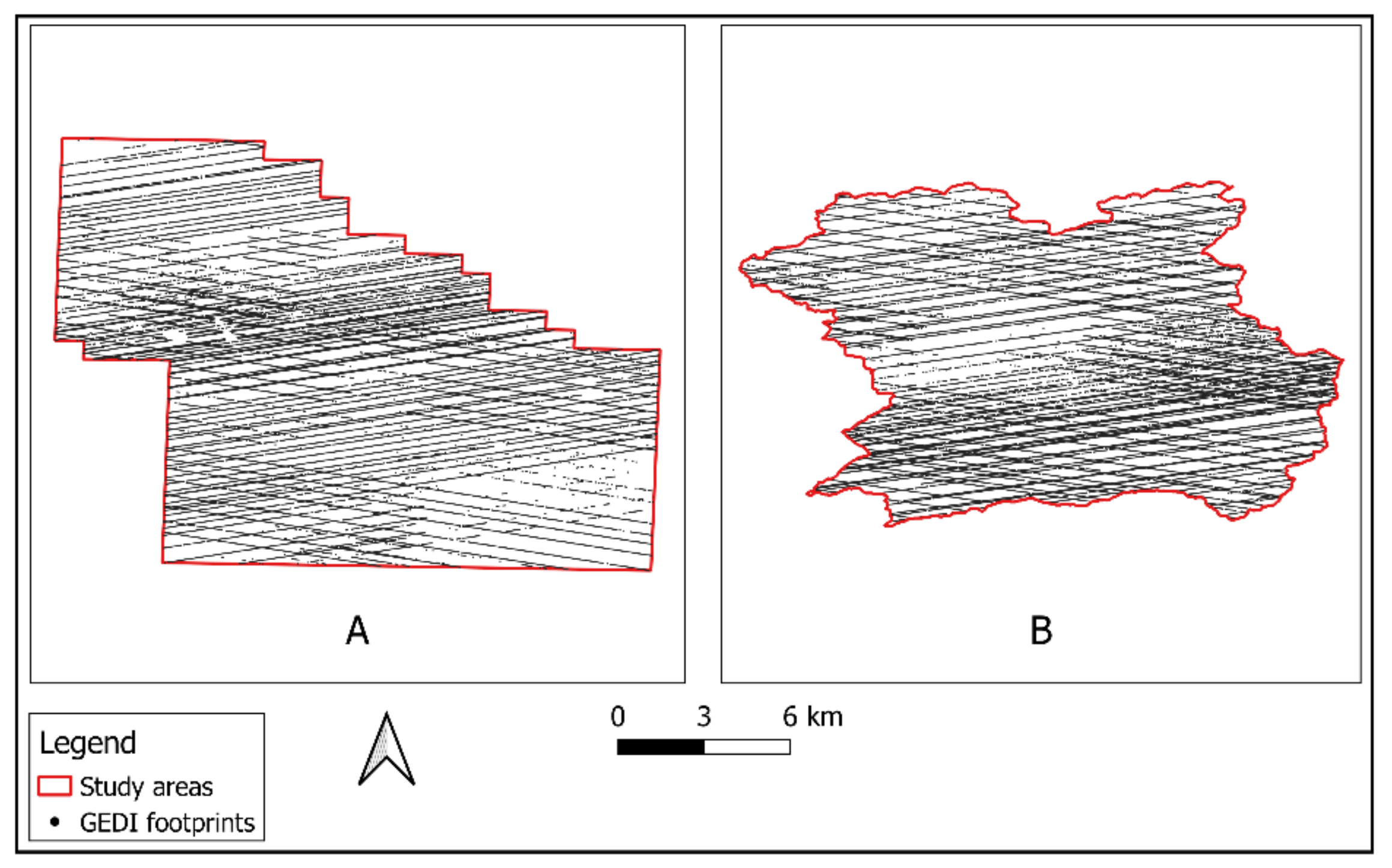
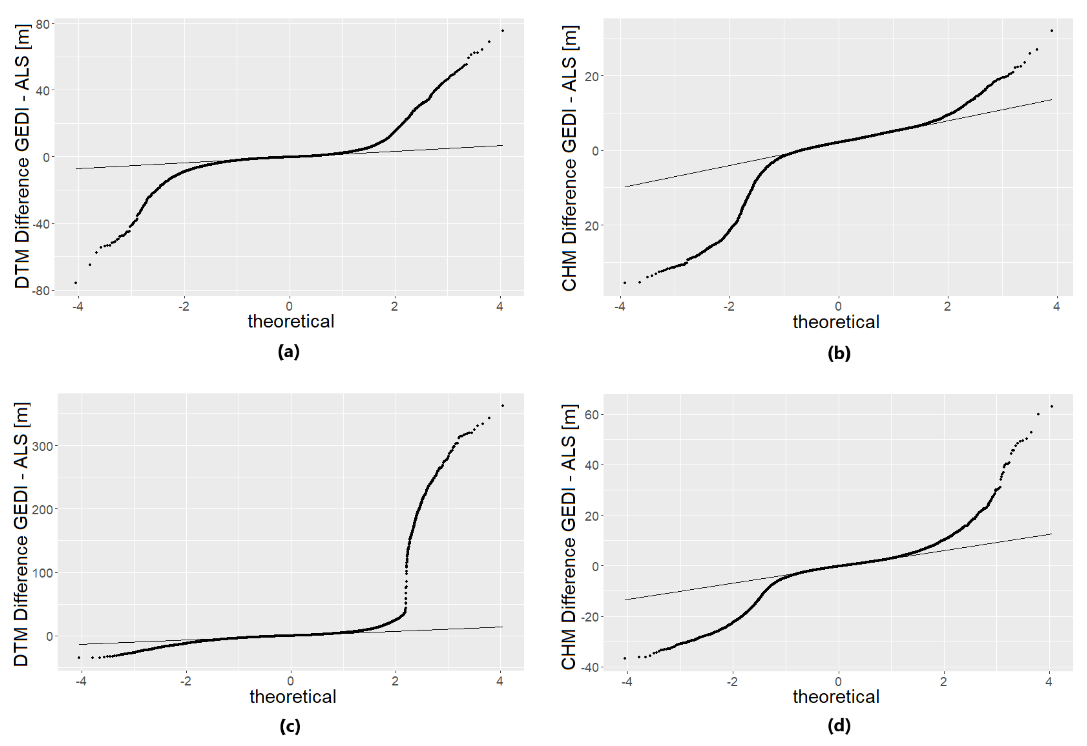
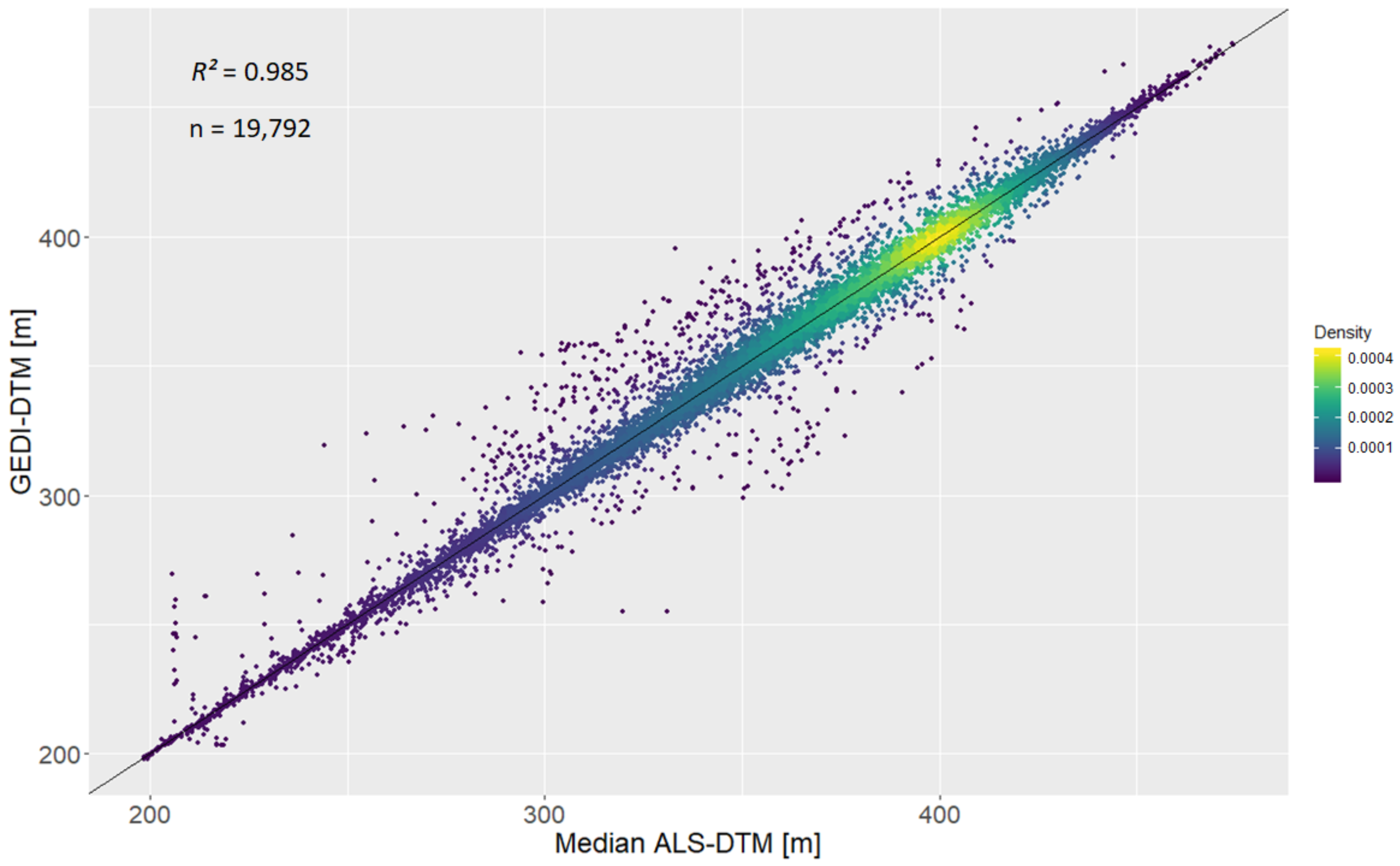
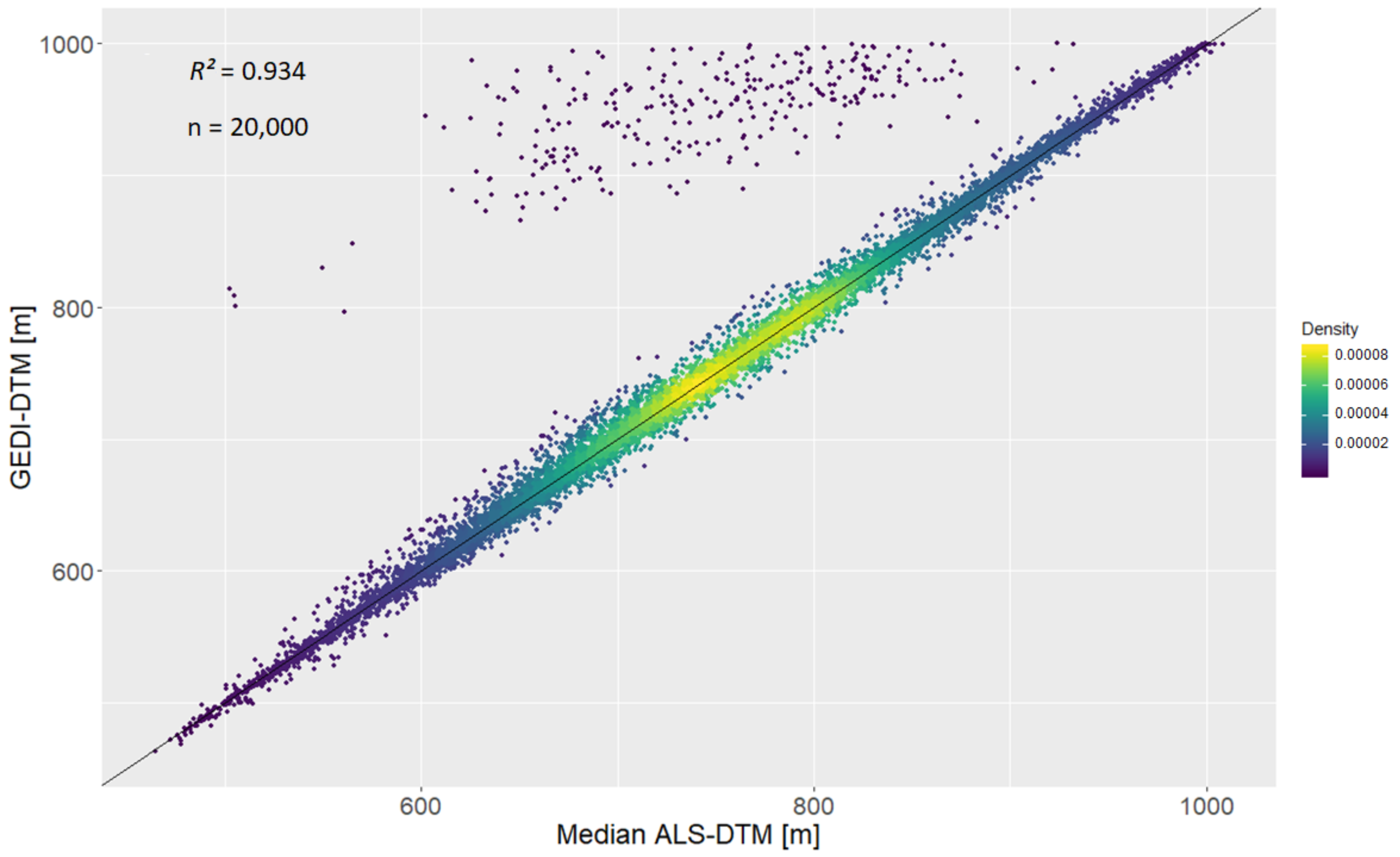
The general statistical analysis of the DTM-differences reveals a relatively low median (and therefore a relatively high accuracy of the GEDI terrain height estimates), but also a high MAD (and therefore a relatively low precision of the GEDI terrain height estimates). The high accuracy is further indicated by the high R2-values, while a number of high outliers, especially in the Thuringian forest area, mirror the relatively low precision. These outliers are dispersed over the study areas and not spatially clustered, though some of them are part of the same orbit-tracks and are therefore spread over the study areas along these tracks.
The median DTM-differences from this study (Roda: −0.26 m, Thuringian forest: 0.18 m) are in the same value range as corresponding mean values from similar studies. Chen [3] found a mean difference of −0.97 m for a study area in North Carolina (using ICESat data), while Wang et al. [32] found a mean difference of −0.61 m for Alaska (using ICESat-2 data). The standard deviation values in both studies were similar to the MAD values found here, however the value range of the DTM-differences was much smaller. In both studies, diverse study areas with various types of land cover and topographies were used. Hilbert and Schmullius [
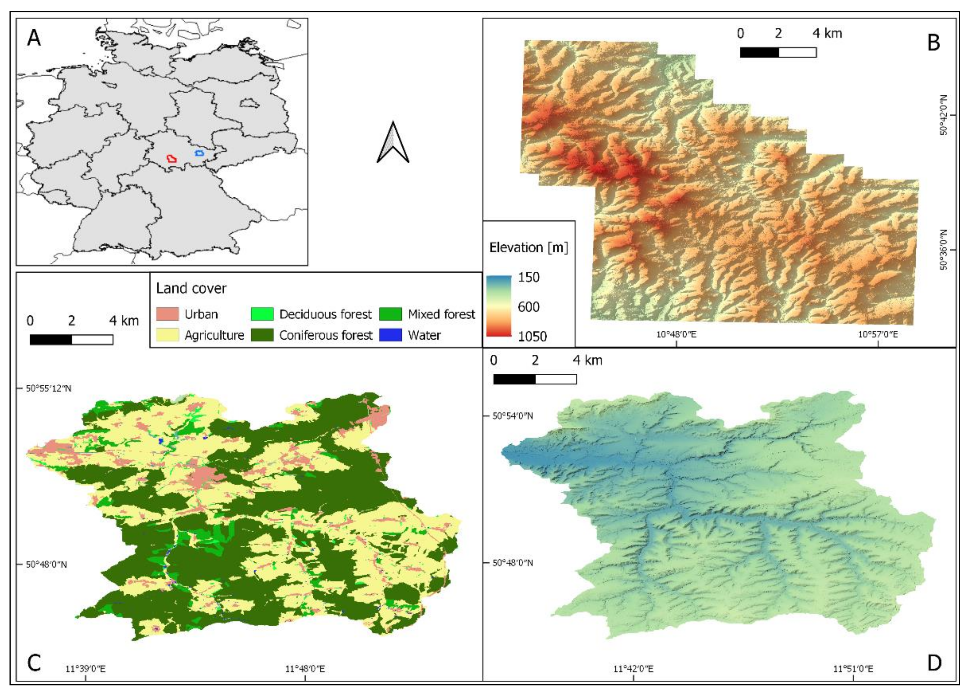
4] analyzed ICESat height estimates in forested and rugged terrain. Their results are especially relevant for this discussion, since their study area is also situated in the Thuringian forest, partially overlapping with the Thuringian forest study area from this study. Using height metrics derived from the ICESat-GLAS GLA01 product, Hilbert and Schmullius calculated a mean difference of 0.19 m compared to a reference ALS-DTM, which is remarkably close to the median of 0.18 m found in this study. Standard deviation of the differences was 5.01 m. In all studies mentioned, the R2 for the correlation between analyzed and reference heights was between 0.98 and 1.
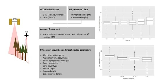
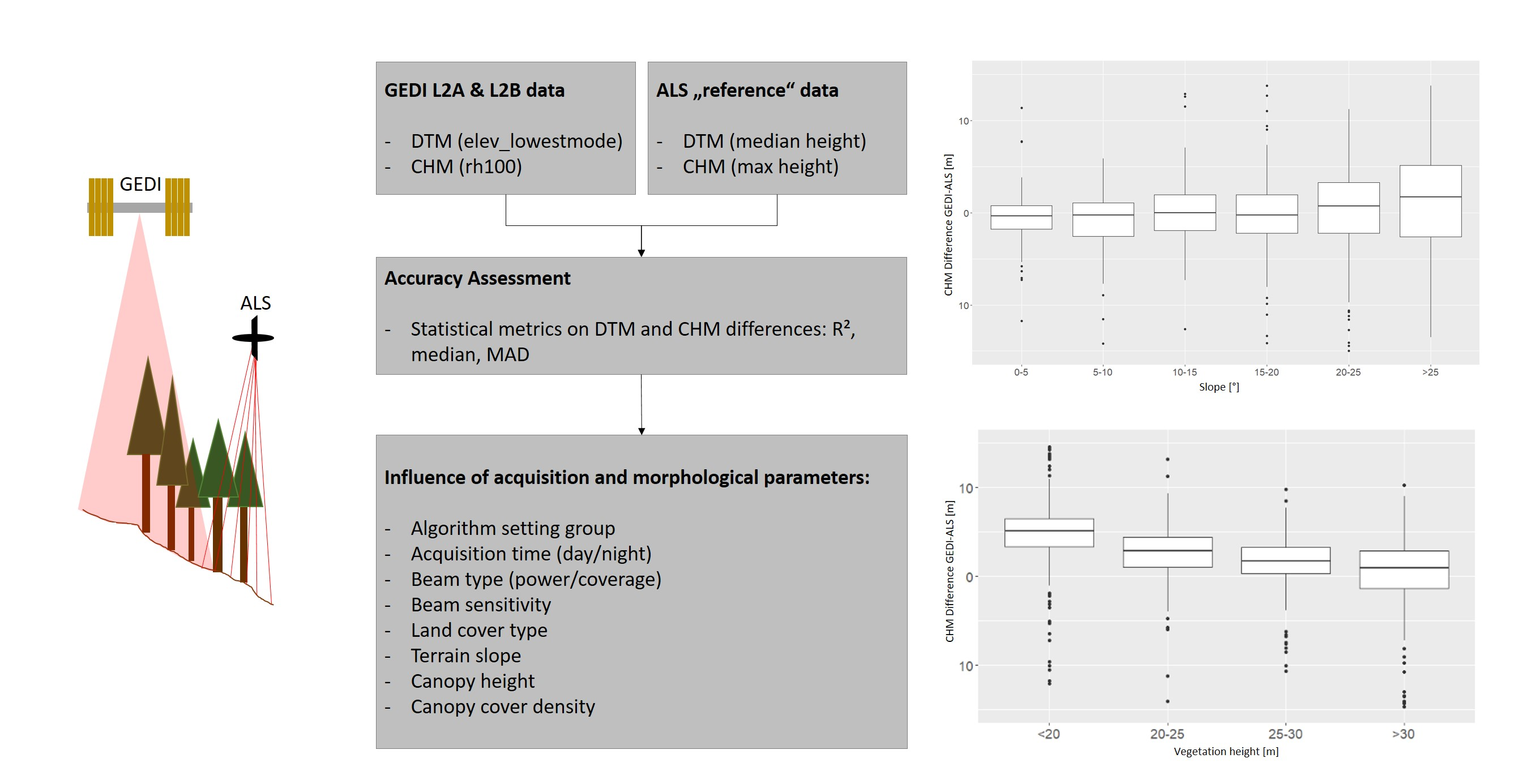
The analysis of the DTM accuracy based on height estimates derived with different algorithm setting groups shows both similarities and differences between the two study areas. The variation of median DTM-differences is higher in the Thuringian forest area. The height metrics from algorithm setting group 1, which are included in the L2B-datasets of the data used here, indeed are the most accurate for the Roda area, but not for the Thuringian forest area. Here, algorithm setting group 3 delivers the most accurate height estimates. In both areas, algorithm setting group 5 delivers a significantly lower accuracy than all other groups. This is caused by its lower waveform signal end threshold compared to the other five setting groups. A low threshold can lead to the detection of noise below the actual ground return signal, resulting in an underestimation of the ground elevation [27]. Algorithms with higher signal end thresholds (e.g., algorithm 1 and 3) are more accurate in this study, allowing the conclusion that these algorithms seem to be preferable for estimating ground elevation in temperate forests. The identical accuracy of algorithm setting groups 1 and 4 is due to the fact that these algorithms only differ in regard to the signal start threshold, which has no effect on ground elevation estimations. It has to be noted that these accuracies are averages over all forest conditions present in these study areas. For the acquisition over more homogenous forests (e.g., with consistently high canopy cover), different algorithms might be preferable.
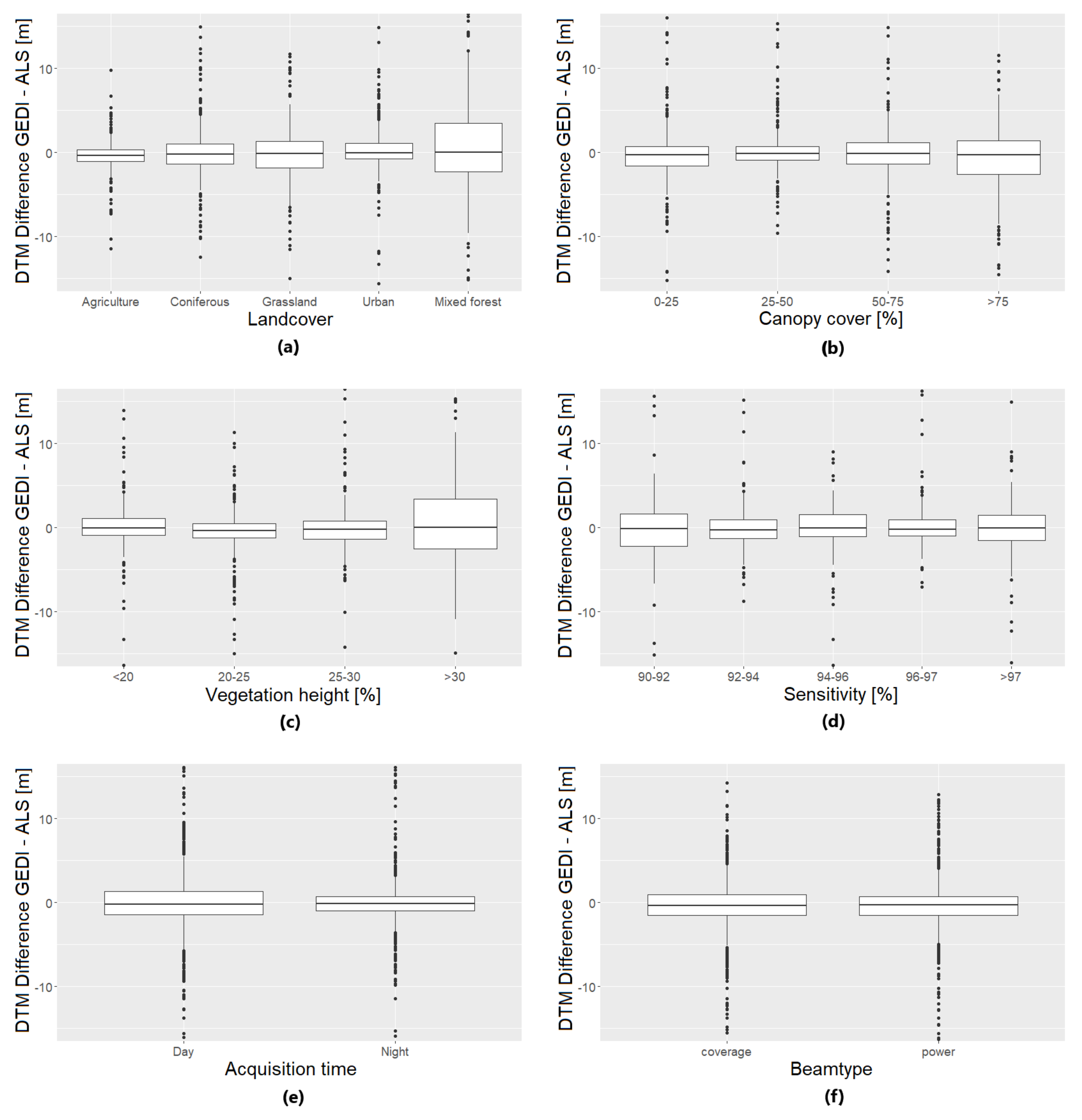
The analysis of the relation between GEDI-DTM accuracy and various environmental and acquisition parameters yields somewhat surprising results. An example is the low influence of land cover within the footprint. Several studies (e.g., Hodgson et al. [37]) observed a lower accuracy of lidar-based DTM over areas with dense/high vegetation. In such areas, the assumption that the lowest mode of a received lidar waveform represents the ground is problematic, since this signal can also stem from low vegetation [38]. However, the results from this study show a slightly higher accuracy of the DTM in mixed forests than in agriculture or grassland areas. The high accuracy of the DTM in urban areas is equally surprising, since those areas are usually challenging when generating lidar-based DTM [39].
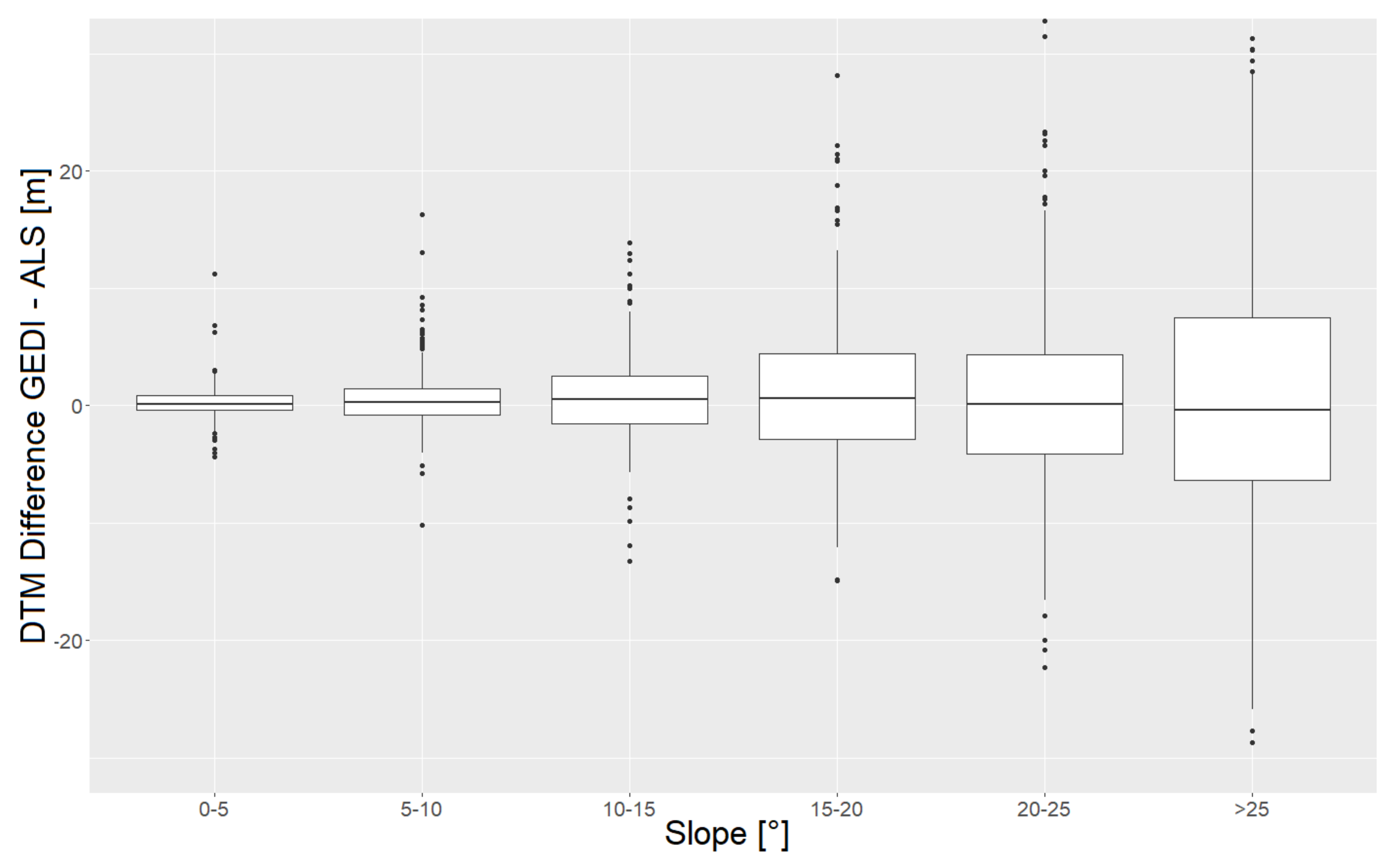
Other results of the analysis are more in accordance with literature. The increased scattering of DTM-differences with increasing slope has been observed in numerous studies [2,32,40]. This effect can occur due to different reasons: on sloped and forested terrain, lidar returns from both vegetation and ground can occur at the same height and therefore might not be distinguishable in the return waveform, especially since the ground returns are spread out over different heights [41]. Also, geolocation errors of footprints can lead to height errors if the footprint area is sloped in the same direction that the footprint is misplaced, since the elevation where the footprint was (falsely) located can be different from the elevation at the actual position of the footprint [42]. This possibility needs to be considered especially for this analysis, given the low current geolocation accuracy of GEDI data. For example, in an area with a slope of 8.31° (which is the mean value of the median slopes within the footprints of the Roda study area), two points along the slope gradient with a horizontal distance of 10 m (which is the lower end of the specified geolocation accuracy of GEDI), have a ground elevation height difference of 1.46 m, while a horizontal distance of 20 m (the upper end of the specified geolocation accuracy of GEDI) results in a ground elevation height difference of 2.92 m. These numbers may give a rough estimation on what scale geolocation errors can influence GEDI DTM accuracy in sloped terrain.
The slight decrease of accuracy with increasing canopy cover within the footprint has also been observed in other studies [32]. This is due the fact that the number of laser impulses that can penetrate the canopy and reach the ground decreases with increasing canopy cover. Stereńczak et al. [43] did not observe an influence of canopy height when analyzing lidar DTM accuracy in a temperate coniferous forest, which is in line with the results found here.
The higher accuracy of height estimates acquired during nighttime can be explained by the lower background noise level (which is increased by sunlight during daytime). This improves the lidar’s capability to detect the ground through dense vegetation [44]. The fact that the beam type of the footprint has almost no influence on DTM accuracy is most likely a result of the overall relatively low density of the forests in the study area. The ability of GEDI’s power beam to penetrate a canopy cover of up to 98% (in comparison to the 95% penetrable by the coverage beam) brings no advantage in this case, since only 20 of the used footprints have a canopy cover of over 95%. The value range of canopy cover values in the Roda area is most likely also the reason for the lack of influence of beam sensitivity on DTM accuracy in this study. Only 16 of the footprints used in the Roda study area have a canopy cover that is higher than their beam sensitivity, meaning that the probability of the laser beam detecting the ground is below 90% for these footprints.
The significantly lower accuracy of height estimates from a number of orbit-tracks in both the Thuringian forest and the Roda study area appears to be not completely explainable. As mentioned, it can be assumed that this result is not caused by one of the parameters whose influence is analyzed here (e.g., an increased slope). The only attribute that is consistent for all footprints of each orbit-track is the acquisition date. Therefore, it could be suspected that certain atmospheric conditions on these dates are the reason for the low accuracy. One parameter of this kind that can influence lidar height estimates is rainfall [45]. While precipitation was indeed recorded in the Thuringian forest area on all three acquisition dates of the orbit-tracks listed in Table 8, no precipitation was recorded in the Roda area on the two acquisition dates of the respective orbit-tracks listed in Table 4 [46].

4.2. GEDI-CHM

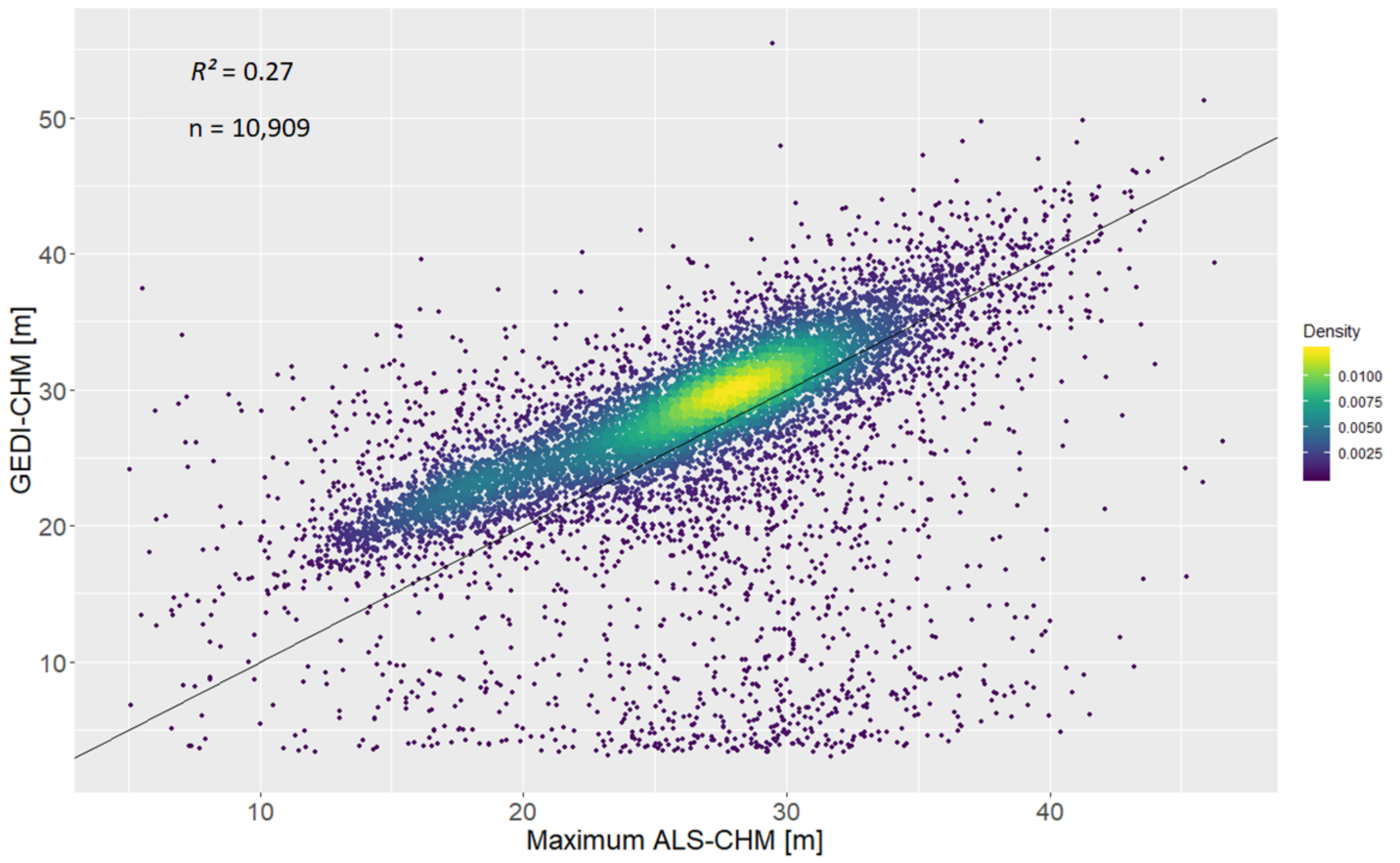
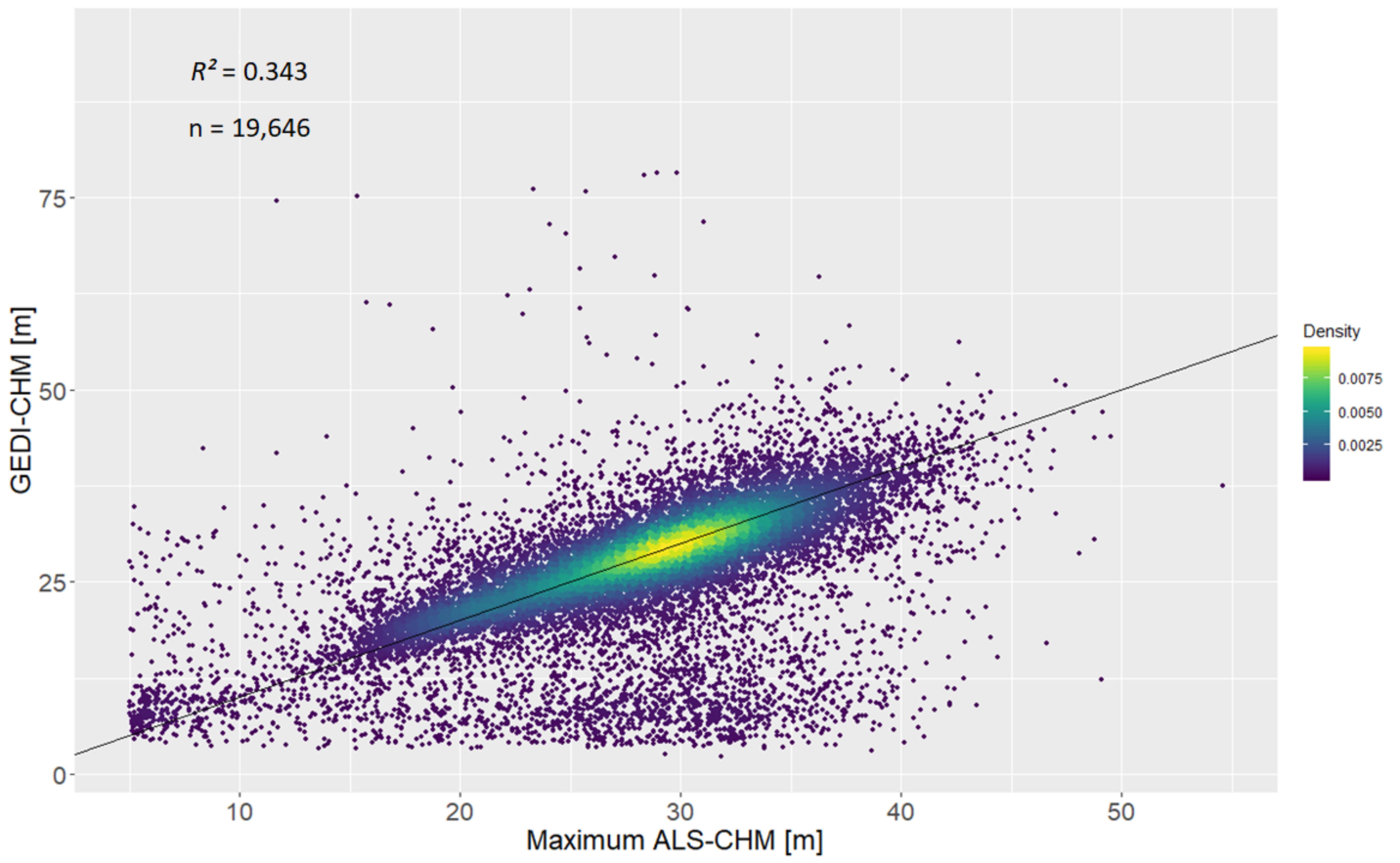
The differences between the two study areas regarding the accuracy of the GEDI-CHM are much larger than for the DTM. While the MAD of the CHM-differences is similar in both areas (with values close to 3), there is a significant difference between the medians: 2.11 m in the Roda area versus −0.23 m in the Thuringian forest area. However, these results are still somewhat in accordance with literature, since the results from similar studies also show rather large differences: while Nie et al. [47] and Popescu et al. [10] observed negative mean differences, Enßle et al. [3], and Hilbert and Schmullius [4] observed positive mean differences. The absolute values of these differences range from 0.2 to 2.5 m, about the same range as the median values observed in this study. It also has to be noted that Hilbert and Schmullius also observed a significantly lower accuracy of the CHM than the DTM derived from the same dataset. Two possible reasons for this generally lower accuracy of CHM compared to DTM are the dependency of CHM accuracy on DTM accuracy and the much more heterogenous surface of the canopy, which requires higher geolocation accuracy of the data.
The differences in the results from the two study areas are also present in the analysis of the algorithm setting groups. While CHM accuracy is still generally higher in the Thuringian forest, this is not the case for every single algorithm. Most notably, algorithm 4 is the second least accurate for the Thuringian forest, but the most accurate for the Roda area. This may be due to its high waveform signal start threshold: the mostly sloped ground of the Thuringian forest means that the return signals from the canopy top are spread out over the return waveform and therefore might not be high enough to surpass the high signal start threshold. This leads to an underestimation of canopy height. It seems that this pattern of high canopy tops not being able to trigger the waveform start in this algorithm is also present in the Roda area. However, in this case it leads to a relatively high accuracy of the algorithm, because this ‘underestimation’ reduces the positive bias of GEDI canopy height estimates that the other algorithms display. Still, the generally higher CHM accuracy in the Thuringian forest area is somewhat surprising, since increased slopes are more known to lead to an overestimation of canopy height (see below). Of course, the accuracy of canopy height estimates derived from waveforms also depends on the accuracy of the ground estimation. For example, the low CHM accuracy of algorithm 5 in both study areas is most likely caused by its low DTM accuracy: here, the underestimation of ground elevation results in a subsequent overestimation of canopy height. The accuracy metrics are also again averages over all forests in the study areas and might be different for specific, more homogenous forest areas.
Certain characteristics of the ALS reference data might have also influenced the results. Small-footprint, discrete return lidar systems tend to underestimate tree heights, especially of coniferous trees, because their laser impulses often miss the top of the tree crowns [38]. The time span between the acquisition of the ALS height estimates and the GEDI height estimates also has to be taken into account when analyzing the GEDI-CHM accuracy. This time difference is consistent for the Roda area (5 years) but varies in the Thuringian forest area (between several months and 4 years). The mean annual height growth rate of the main tree types in the Roda area (pine and spruce) varies between 20–60 cm [48,
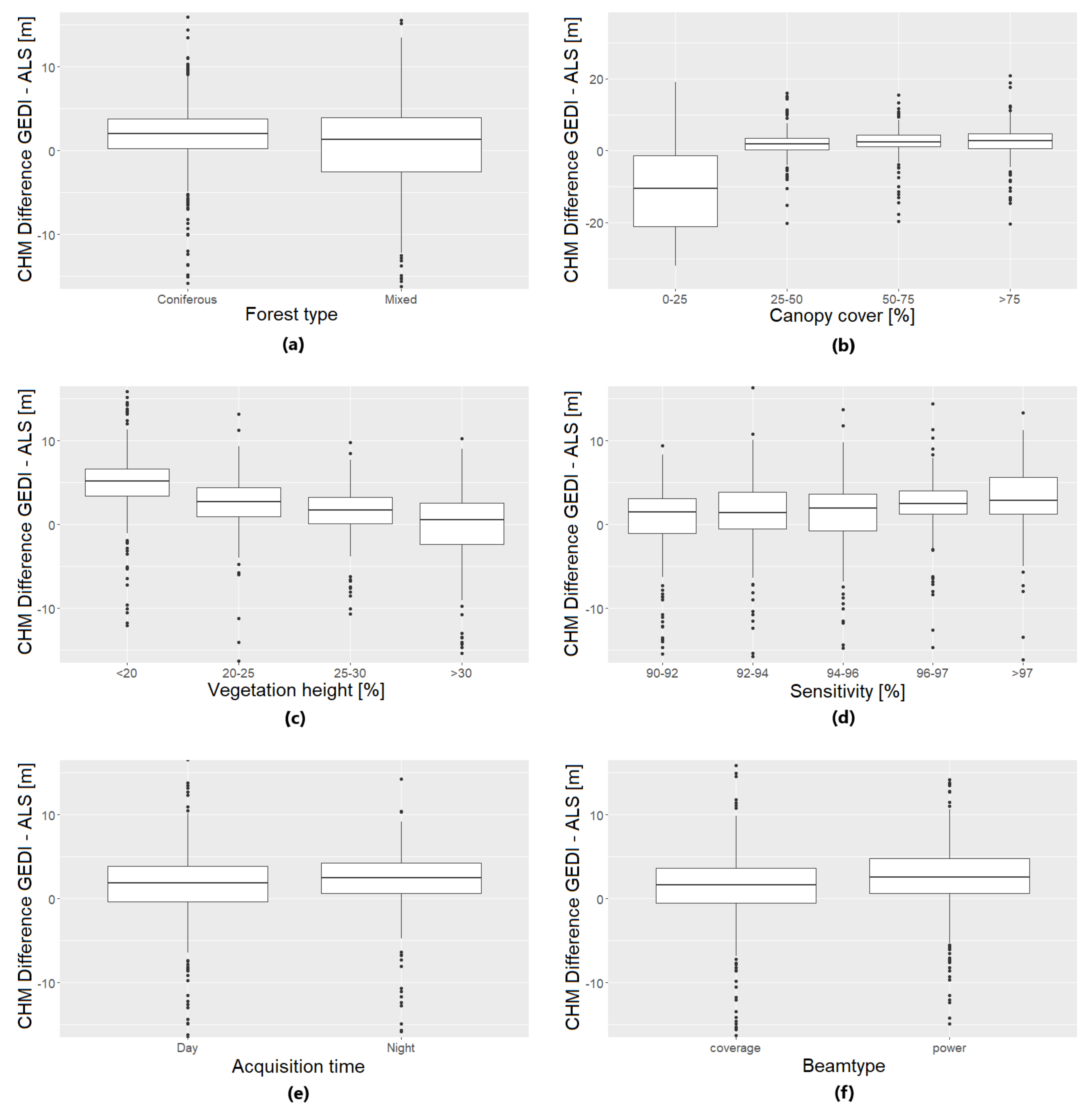
49]. A mean annual height growth of 40 cm would amount to 2 m in 5 years. Therefore, it seems at least possible that the median CHM-difference of around 2 m can be explained to a certain degree by the height increase of the canopy between the acquisition dates. Another result that might suggest this is the apparent influence of vegetation height on CHM accuracy. In general, the annual height growth of trees slows down after the trees reach a certain age (depending on tree type and environmental factors) [50]. This might explain why the median CHM-difference in this study is much higher for shorter (presumably younger) trees than for taller (presumably older) trees (Table 11), assuming they experienced a larger height increase between the acquisition dates. However, this difference in accuracy appears to be too large to be solely explainable by height growth differences, and therefore may not be adequate to accurately quantify the influence of the acquisition time difference on GEDI-CHM accuracy. Also, there is no significant influence of acquisition time differences in the Thuringian forest area. Here, CHM accuracy does not significantly decrease with increasing time difference between the GEDI and ALS acquisitions (Table 12). It also has to be noted that while the relation between CHM accuracy and vegetation height can be used to at least roughly assess whether vegetation growth between the acquisition dates had an effect on CHM accuracy, this does not give indications as to whether potential changes in land cover between the acquisitions might have influenced the results. There is, however, the possibility that the logging of trees in the Roda study area in June 2019 is the reason for at least some of the observed negative outliers.
The analysis of GEDI-CHM accuracy with regard to environmental and acquisition parameters shows, in some cases, discrepancies with the results from other studies. As an example, many studies [51,52] observe a higher accuracy of lidar CHM in coniferous forests than in deciduous or mixed forests. This is because deciduous forests (during leaf-on conditions) tend to have a more closed structure with less gaps for the laser impulse to detect the ground through [4]. This could at least explain the higher MAD over mixed forests observed in this study.
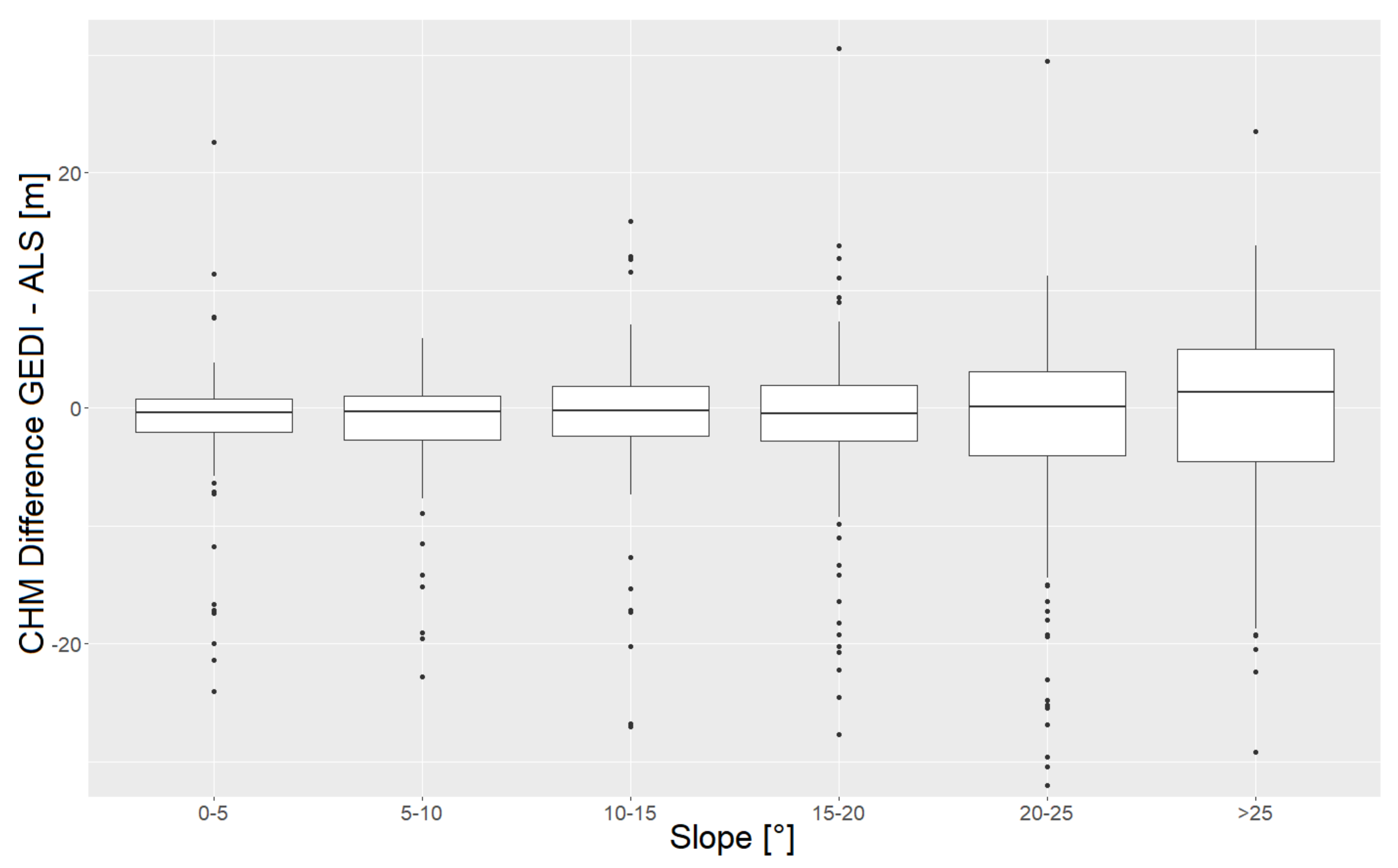
The increased MAD of the CHM-differences in areas with steeper slopes in the Thuringian forest study area is more in accordance with literature. Hilbert and Schmullius [4] observed a similar trend in an adjacent study area, using ICESat-GLAS canopy height estimates. Aside from the reasons for this effect that are stated in Section 4.1 (regarding the influence of slope on DTM accuracy), increasing slopes also lead to an increased lidar waveform extent [53]. This can lead to an overestimation of canopy height if the canopy height is derived from the height differences between the waveform signal start and the ground elevation.
The significantly lower CHM accuracy in areas with a canopy cover lower than 25% may be due to several reasons: in sloped areas with low canopy cover, the return signals from the canopy top might not exceed the waveform recording start threshold, so the waveform recording is triggered by lower canopy layers or ground return signals. In this case, the height difference between the waveform signal start and the ground elevation is lower or (close to) zero. In addition, if the vegetation is concentrated in the lower part of a sloped area, the waveform recording might also be triggered by ground surface from the upper part of the area, which has a higher elevation than the canopy top [3]. The relatively low horizontal geolocation accuracy of GEDI footprints can also reduce CHM accuracy in areas with low and heterogenous canopy cover, if a footprint that covered vegetation is falsely located in an area with bare land, or vice versa. As Table 13 shows, accuracy in areas with low canopy cover (<25%) improves when only footprints in flat terrain (median slope <3°) are considered, suggesting that slope is the dominant factor influencing CHM accuracy in areas with low canopy cover. The difference in accuracy between areas with low and high canopy cover that is still present in flat terrain (Table 13) is most likely caused by geolocation errors, therefore giving a rough estimation on the influence of these errors on GEDI CHM accuracy.
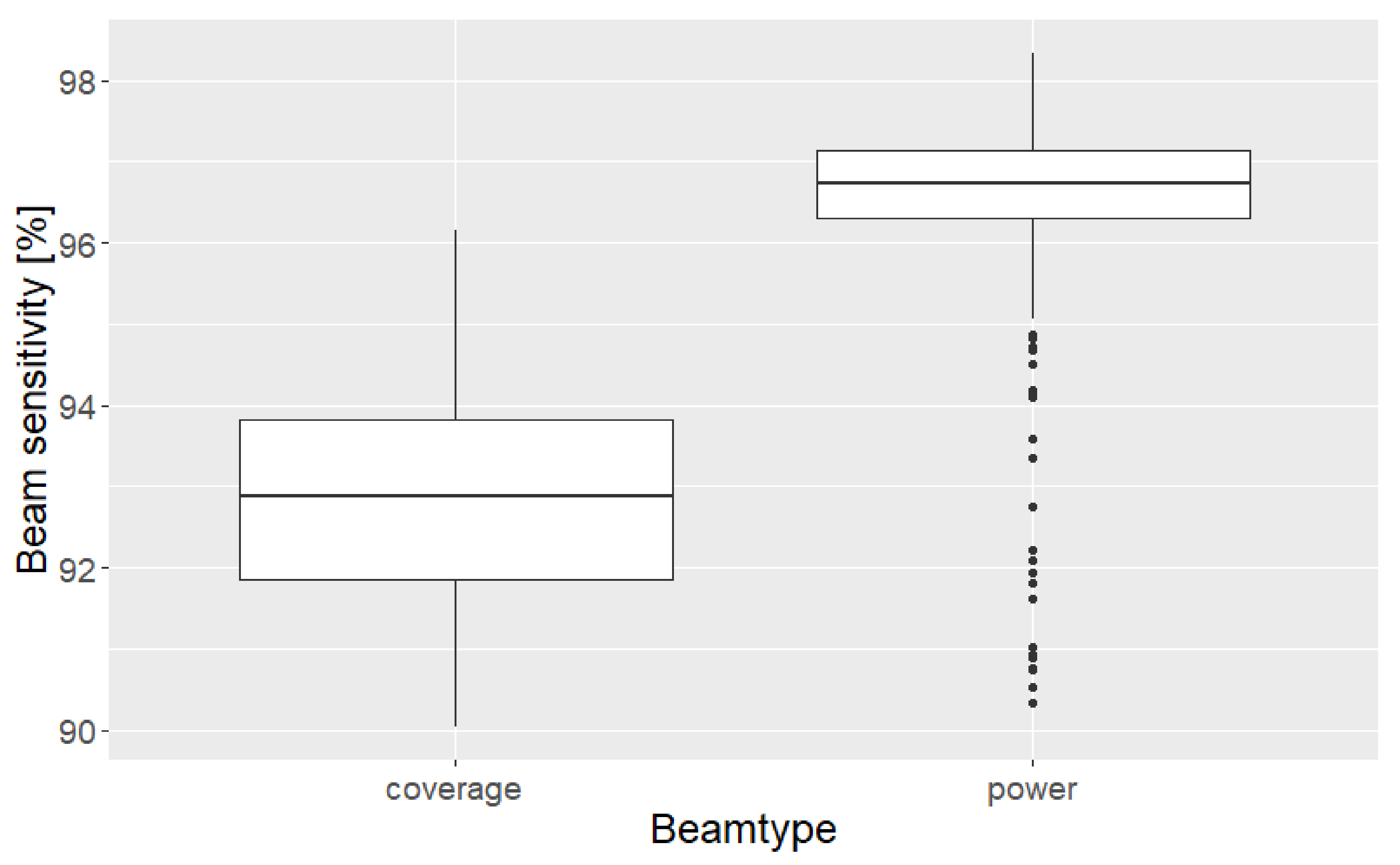
The influence of acquisition time and beam type on CHM accuracy is generally similar to the results from the DTM, with the exception of the lower median of CHM differences from coverage beams compared to power beams. This may be connected to the increased median beam sensitivity of power beams (Figure 13). For the dataset used here, the median CHM-difference increases with increasing beam sensitivity.
The connection between beam sensitivity and beamtype does not explain the increase of median CHM-differences with increasing beam sensitivity. As mentioned in Section 4.1, the number of footprints where the beam sensitivity could have an influence on CHM accuracy is small, and, if anything, a positive influence of increasing beam sensitivity on CHM accuracy was to be expected. This may lead to the conclusion that beam sensitivity correlates with another parameter that has an influence on the accuracy. However, no parameter included in this analysis shows a noteworthy correlation with beam sensitivity (the highest being the correlation with slope, with a Pearsons’s r of −0.11).
As with the DTM, the low accuracy of height estimates from certain footprints in both the Roda and Thuringian forest area cannot be fully explained, with the influence of rainfall during the acquisition only being a possible explanation for the Thuringian forest footprints. In addition, values that form clusters of outliers in the scatterplots (Figure 7 and Figure 11) are dispersed over the study areas and not spatially clustered.

5. Conclusions

The results of the analysis presented in this study show both similarities and differences to the results of comparable studies. GEDI ground elevation metrics have a relatively high accuracy, with median DTM-differences below 30 cm. These values suggest an increased accuracy compared to the results from studies using other spaceborne lidar-based height metrics. However, the MAD of the DTM-differences are relatively high, indicating a relatively low measurement precision. While the analysis of the different algorithm setting groups for the calculation of ground elevation metrics did not point to a single most accurate group, it can be concluded that algorithms with a high waveform signal end threshold seem to be preferable for deriving ground elevation over temperate forests.
The analysis of the influence of various environmental and acquisition parameters shows that GEDI-DTM accuracy stays more or less constant under most conditions. Certain characteristics of lidar-based height metrics (e.g., a decrease in accuracy with increasing slope or a higher accuracy of nighttime acquisitions) can be confirmed in GEDI elevation height metrics, while others (e.g., a lower accuracy over forests and urban areas in comparison to open fields) cannot be corroborated with the analyzed datasets. However, only steep slopes seem to lead to a significant decline in accuracy. Also, for the ground elevation estimates over temperate forests analyzed in this study, differences in beamtype and sensitivity of the GEDI beams do not affect the accuracy.
GEDI canopy height metrics are less accurate than elevation heights, with much higher medians and MAD of the differences to reference heights and a much lower correlation. Apart from the more complex surface of canopy, some of the results suggest that changes of the vegetation (growth and logging) may have influenced these results, due to the time difference between the acquisition of GEDI and reference data. The differences in accuracy between the two study areas as well as the algorithm setting groups are larger than for the DTM, with a generally higher accuracy in the more mountainous Thuringian forest area. Though comparability is somewhat limited, the results show a similar accuracy compared to the results from other studies. Less similarities are found in the analysis of CHM accuracy with regard to environmental and acquisition parameters. While the reduced accuracy over areas with low canopy cover or in steep slopes follows expected and previously observed patterns, other parameters show less expectable (and explainable) influences. Among those are a higher accuracy over mixed than over coniferous forests and especially the decreasing accuracy with increasing beam sensitivity.
In addition, the significantly lower accuracy of the footprints from certain orbit-tracks (both for the DTM and the CHM) remains surprising, since none of the variables considered in this analysis (including rainfall) hold a complete explanation for these results. Finally, the observed influence of parameters like slope or canopy cover, whose values can vary spatially on the scale of GEDI geolocation accuracy, suggest that the results for both DTM and CHM accuracy are to a certain degree influenced by GEDI geolocation errors and will probably be improved in further versions.
It can be concluded that GEDI ground elevation estimates show a slightly increased accuracy compared to the results from earlier studies, while no clear improvement could be observed for the canopy height estimates. In general, GEDI height metrics have the potential to be used as a solid basis for further investigations and applications that require large scale ground elevation or canopy height information. At the same time, some of the observed characteristics of GEDI height estimates remain unexplained. Whether these are isolated cases unique to the datasets analyzed here, or general characteristics of GEDI data, can only be determined with further investigations of GEDI lidar performance under different environmental and acquisition conditions. Further research might also address or compensate for some of the factors that might have influenced the results from this study, like geolocation accuracy of GEDI data (which is expected to improve in the future), or potential errors and acquisition time differences in the reference data.

Author Contributions

Conceptualization, M.U. and C.D.; Methodology, M.A., M.U. and C.D.; Validation, M.A.; Formal analysis, M.A.; Investigation, M.A.; Resources, M.U.; Data curation, M.A. and M.U.; Writing—original draft preparation, M.A.; Writing—review and editing, M.U. and C.D.; Visualization, M.A.; Supervision, M.U. and C.D.; Project administration, M.U., C.D. and C.S. All authors have read and agreed to the published version of the manuscript.

Funding

This research received no external funding.

Acknowledgments

The authors would like to thank NASA and University of Maryland for providing spaceborne GEDI data and Thuringian land surveying office for providing ALS and land cover data. M.U. was supported in part by the 2017–2018 Belmont Forum and BiodivERsA joint call for research proposals, under the BiodivScen ERA-Net COFUND program, and in part by the funding organization of the German Federal Ministry of Education and Research (BMBF) under grant no. 01LC1808A. The authors also thank two anonymous reviewers for their helpful and valuable comments.

Conflicts of Interest

The authors declare no conflict of interest.

Appendix A

Appendix A.1. Tables Containing Accuracy Metrics of the GEDI DTM

Table A1. Accuracy metrics of GEDI DTM height estimates depending on land cover (Roda study area).
Land CoverMedian DTM-Difference (m)MAD DTM-Difference (m)
Agriculture−0.321.02
Coniferous forest−0.191.77
Grassland−0.162.34
Mixed forest−0.0054.34
Urban−0.0591.24
Table A2. Accuracy metrics of GEDI DTM height estimates depending on canopy cover (Roda study area).
Canopy Cover (%)Median DTM-Difference (m)MAD DTM-Difference (m)
0–25−0.291.75
25–50−0.151.22
50–75−0.151.85
>75−0.313.06
Table A3. Accuracy metrics of GEDI DTM height estimates depending on canopy height (Roda study area).
Canopy Height (m)Median DTM-Difference (m)MAD DTM-Difference (m)
<20−0.041.47
20–25−0.371.29
25–30−0.171.62
>300.014.44
Table A4. Accuracy metrics of GEDI DTM height estimates depending on beam sensitivity (Roda study area).
Beam Sensitivity (%)Median DTM-Difference (m)MAD DTM-Difference (m)
90–92−0.093.06
92–94−0.301.87
94–96−0.052.03
96–97−0.211.42
>97−0.072.19
Table A5. Accuracy metrics of GEDI DTM height estimates depending on acquisition time (Roda study area).
Acquisition TimeMedian DTM-Difference (m)MAD DTM-Difference (m)
Day−0.232.08
night−0.121.24
Table A6. Accuracy metrics of GEDI DTM height estimates depending on beam type (Roda study area).
Beam TypeMedian DTM-Difference (m)MAD DTM-Difference (m)
Coverage−0.351.78
power−0.281.65
Table A7. Accuracy metrics of GEDI DTM height estimates depending on slope (Thuringian forest study area).
Slope (°)Median DTM-Difference (m)MAD DTM-Difference (m)
0–50.090.95
5–100.261.67
10–150.552.97
15–200.655.45
20–250.086.32
>25−0.3910.82

Appendix A.2. Tables Containing Accuracy Metrics of the GEDI CHM

Table A8. Accuracy metrics of GEDI canopy height estimates depending on forest type (Roda study area).
Forest TypeMedian CHM-Difference (m)MAD CHM-Difference (m)
Coniferous2.002.64
Mixed1.334.39
Table A9. Accuracy metrics of GEDI canopy height estimates depending on canopy cover (Roda study area).
Canopy Cover (%)Median CHM-Difference (m)MAD CHM-Difference (m)
0–25−10.4714.41
25–501.852.43
50–752.442.16
>752.733.05
Table A10. Accuracy metrics of GEDI canopy height estimates depending on canopy height (Roda study area).
Canopy Height (m)Median CHM-Difference (m)MAD CHM-Difference (m)
<205.152.51
20–252.752.61
25–301.692.31
>300.543.63
Table A11. Accuracy metrics of GEDI canopy height estimates depending on beam sensitivity (Roda study area).
Beam Sensitivity (%)Median CHM-Difference (m)MAD CHM-Difference (m)
90–921.512.99
92–941.423.20
94–961.973.42
96–972.492.04
>972.883.03
Table A12. Accuracy metrics of GEDI canopy height estimates depending on acquisition time (Roda study area).
Acquisition TimeMedian CHM-Difference (m)MAD CHM-Difference (m)
Day1.903.13
Night2.502.67
Table A13. Accuracy metrics of GEDI canopy height estimates depending on beam type (Roda study area).
Beam TypeMedian CHM-Difference (m)MAD CHM-Difference (m)
Coverage1.653.17
Power2.603.06
Table A14. Accuracy metrics of GEDI canopy height estimates depending on slope (Thuringian forest study area).
Slope (°)Median CHM-Difference (m)MAD CHM-Difference (m)
0–5−0.402.06
5–10−0.292.85
10–15−0.223.22
15–20−0.463.59
20–250.135.02
>251.406.03

References

  1. Schutz, B.E.; Zwally, H.J.; Shuman, C.A.; Hancock, D.; DiMarzio, J.P. Overview of the ICESat Mission. Geophys. Res. Lett. 2005, 32. [Google Scholar] [CrossRef] [Green Version]
  2. Enßle, F.; Heinzel, J.; Koch, B. Accuracy of vegetation height and terrain elevation derived from ICESat/GLAS in forested areas. Int. J. Appl. Earth Obs. Geoinf. 2014, 31, 37–44. [Google Scholar] [CrossRef]
  3. Chen, Q. Assessment of terrain elevation derived from satellite laser altimetry over mountainous forest areas using airborne lidar data. ISPRS J. Photogramm. Remote Sens. 2010, 65, 111–122. [Google Scholar] [CrossRef]
  4. Hilbert, C.; Schmullius, C. Influence of Surface Topography on ICESat/GLAS Forest Height Estimation and Waveform Shape. Remote Sens. 2012, 4, 2210–2235. [Google Scholar] [CrossRef] [Green Version]
  5. Hayashi, M.; Saigusa, N.; Oguma, H.; Yamagata, Y. Forest canopy height estimation using ICESat/GLAS data and error factor analysis in Hokkaido, Japan. ISPRS J. Photogramm. Remote Sens. 2013, 81, 12–18. [Google Scholar] [CrossRef]
  6. Fang, Z.; Cao, C. Estimation of Forest Canopy Height over Mountainous Areas Using Satellite Lidar. IEEE J. Sel. Top. Appl. Earth Obs. Remote Sens. 2014, 7, 3157–3166. [Google Scholar] [CrossRef]
  7. Mahoney, C.; Hopkinson, C.; Held, A.; Kljun, N.; van Gorsel, E. ICESat/GLAS Canopy Height Sensitivity Inferred from Airborne Lidar. Photogramm. Eng. Remote Sens. 2016, 82, 351–363. [Google Scholar] [CrossRef]
  8. Lefsky, M.A.; Harding, D.J.; Keller, M.; Cohen, W.B.; Carabajal, C.C.; Del Bom Espirito-Santo, F.; Hunter, M.O.; de Oliveira, R. Estimates of forest canopy height and aboveground biomass using ICESat. Geophys. Res. Lett. 2005, 32. [Google Scholar] [CrossRef] [Green Version]
  9. Boudreau, J.; Nelson, R.; Margolis, H.; Beaudoin, A.; Guindon, L.; Kimes, D. Regional aboveground forest biomass using airborne and spaceborne LiDAR in Québec. Remote Sens. Environ. 2008, 112, 3876–3890. [Google Scholar] [CrossRef]
  10. Popescu, S.C.; Zhao, K.; Neuenschwander, A.; Lin, C. Satellite lidar vs. small footprint airborne lidar: Comparing the accuracy of aboveground biomass estimates and forest structure metrics at footprint level. Remote Sens. Environ. 2011, 115, 2786–2797. [Google Scholar] [CrossRef]
  11. Lefsky, M.A. A global forest canopy height map from the Moderate Resolution Imaging Spectroradiometer and the Geoscience Laser Altimeter System. Geophys. Res. Lett. 2010, 37. [Google Scholar] [CrossRef] [Green Version]
  12. Simard, M.; Pinto, N.; Fisher, J.B.; Baccini, A. Mapping forest canopy height globally with spaceborne lidar. J. Geophys. Res. 2011, 116. [Google Scholar] [CrossRef] [Green Version]
  13. Pang, Y.; Lefsky, M.; Sun, G.; Ranson, J. Impact of footprint diameter and off-nadir pointing on the precision of canopy height estimates from spaceborne lidar. Remote Sens. Environ. 2011, 115, 2798–2809. [Google Scholar] [CrossRef]
  14. Dubayah, R.; Blair, J.B.; Goetz, S.; Fatoyinbo, L.; Hansen, M.; Healey, S.; Hofton, M.; Hurtt, G.; Kellner, J.; Luthcke, S.; et al. The Global Ecosystem Dynamics Investigation: High-resolution laser ranging of the Earth’s forests and topography. Sci. Remote Sens. 2020, 1, 100002. [Google Scholar] [CrossRef]
  15. Qi, W.; Saarela, S.; Armston, J.; Ståhl, G.; Dubayah, R. Forest biomass estimation over three distinct forest types using TanDEM-X InSAR data and simulated GEDI lidar data. Remote Sens. Environ. 2019, 232, 111283. [Google Scholar] [CrossRef]
  16. Duncanson, L.; Neuenschwander, A.; Hancock, S.; Thomas, N.; Fatoyinbo, T.; Simard, M.; Silva, C.A.; Armston, J.; Luthcke, S.B.; Hofton, M.; et al. Biomass estimation from simulated GEDI, ICESat-2 and NISAR across environmental gradients in Sonoma County, California. Remote Sens. Environ. 2020, 242, 111779. [Google Scholar] [CrossRef]
  17. Rödiger, T. Charakterisierung und Modellierung des Buntsandsteinfließsystems im Osten des Thüringer Beckens. Ph.D. Thesis, Friedrich-Schiller-University Jena, Jena, Germany, 2005. [Google Scholar]
  18. Thiel, C.; Müller, M.M.; Berger, C.; Cremer, F.; Dubois, C.; Hese, S.; Baade, J.; Klan, F.; Pathe, C. Monitoring Selective Logging in a Pine-Dominated Forest in Central Germany with Repeated Drone Flights Utilizing A Low Cost RTK Quadcopter. Drones 2020, 4, 11. [Google Scholar] [CrossRef] [Green Version]
  19. Thüringer Ministerium für Landwirtschaft, Naturschutz und Umwelt (TMLNU). Bericht zur Überprüfung des UNESCO-Biosphärenreservates “Vessertal—Thüringer Wald"; TMLNU: Erfurt, Germany, 2003. [Google Scholar]
  20. Natural Earth. Admin 0—Countries. Available online: https://www.naturalearthdata.com/downloads/50m-cultural-vectors/ (accessed on 11 November 2020).
  21. DIVA-GIS. DEU_adm. Available online: https://www.diva-gis.org/gdata (accessed on 6 October 2020).
  22. Thüringer Landesamt für Bodenmanagement und Geoinformation (TLBG). Höhendaten. Available online: https://www.geoportal-th.de/de-de/Downloadbereiche/Download-Offene-Geodaten-Th%C3%BCringen/Download-H%C3%B6hendaten (accessed on 1 June 2020).
  23. Thüringer Landesamt für Bodenmanagement und Geoinformation (TLBG). ATKIS Basis-DLM, Thüringen komplett. Available online: https://www.geoportal-th.de/de-de/Downloadbereiche/Download-Offene-Geodaten-Th%C3%BCringen/Download-ATKIS-Basis-DLM (accessed on 18 May 2020).
  24. Dubayah, R.; Hofton, M.; Blair, J.B.; Armston, J.; Tang, H.; Luthcke, S. GEDI L2A Elevation and Height Metrics Data Global Footprint Level V001. NASA EOSDIS Land Processes DAAC. Available online: https://0-doi-org.brum.beds.ac.uk/10.5067/GEDI/GEDI02_A.001 (accessed on 10 August 2020).
  25. Dubayah, R.; Tang, H.; Armston, J.; Luthcke, S.; Hofton, M.A.; Blair, J.B. GEDI L2B Canopy Cover and Vertical Profile Metrics Data Global Footprint Level V001. NASA EOSDIS Land Processes DAAC. Available online: https://0-doi-org.brum.beds.ac.uk/10.5067/GEDI/GEDI02_B.001 (accessed on 10 August 2020).
  26. Hancock, S.; Armston, J.; Hofton, M.; Sun, X.; Tang, H.; Duncanson, L.I.; Kellner, J.R.; Dubayah, R. The GEDI Simulator: A Large-Footprint Waveform Lidar Simulator for Calibration and Validation of Spaceborne Missions. Earth Space Sci. 2019, 6, 294–310. [Google Scholar] [CrossRef]
  27. Hofton, M.A.; Blair, J.B. Algorithm Theoretical Basis Document (ATBD) for GEDI Transmit and Receive Waveform Processing for L1 and L2 Products. Available online: https://lpdaac.usgs.gov/documents/581/GEDI_WF_ATBD_v1.0.pdf (accessed on 20 June 2020).
  28. Tang, H.; Armston, J. Algorithm Theoretical Basis Document (ATBD) for GEDI L2B Footprint Canopy Cover and Vertical Profile Metrics. Available online: https://lpdaac.usgs.gov/documents/588/GEDI_FCCVPM_ATBD_v1.0.pdf (accessed on 20 June 2020).
  29. Thüringer Landesamt für Bodenmanagement und Geoinformation (TLBG).Geobasisdaten; TLBG Produktverzeichnis No. 2, 2018. Available online: https://www.thueringen.de/de/publikationen/pic/pubdownload1547.pdf (accessed on 2 June 2020).
  30. R Core Team. R: A Language and Environment for Statistical Computing; R Foundation for Statistical Computing: Vienna, Austria, 2018. [Google Scholar]
  31. Wickham, H.; Averick, M.; Bryan, J.; Chang, W.; McGowan, L.; François, R.; Grolemund, G.; Hayes, A.; Henry, L.; Hester, J.; et al. Welcome to the Tidyverse. JOSS 2019, 4, 1686. [Google Scholar] [CrossRef]
  32. Wang, C.; Zhu, X.; Nie, S.; Xi, X.; Li, D.; Zheng, W.; Chen, S. Ground elevation accuracy verification of ICESat-2 data: A case study in Alaska, USA. Opt. Express 2019, 27, 38168–38179. [Google Scholar] [CrossRef]
  33. Wellhausen, K.; Heym, M.; Pretzsch, M. Mischbestände aus Kiefer (Pinus sylvestris L.) und Fichte (Picea abies (KARST.) L.): Ökologie, Ertrag und waldbauliche Behandlung. Allg. Forst-und Jagdztg. 2017, 188, 3–34. [Google Scholar]
  34. Escobar Villanueva, J.R.; Iglesias Martínez, L.; Pérez Montiel, J.I. DEM Generation from Fixed-Wing UAV Imaging and LiDAR-Derived Ground Control Points for Flood Estimations. Sensors 2019, 19. [Google Scholar] [CrossRef] [PubMed] [Green Version]
  35. Höhle, J.; Höhle, M. Accuracy assessment of digital elevation models by means of robust statistical methods. ISPRS J. Photogramm. Remote Sens. 2009, 64, 398–406. [Google Scholar] [CrossRef] [Green Version]
  36. Rousseeuw, P.J.; Croux, C. Alternatives to the Median Absolute Deviation. J. Am. Stat. Assoc. 1993, 88, 1273–1283. [Google Scholar] [CrossRef]
  37. Hodgson, M.E.; Jensen, J.; Raber, G.; Tullis, J.; Davis, B.A.; Thompson, G.; Schuckman, K. An Evaluation of Lidar-derived Elevation and Terrain Slope in Leaf-off Conditions. Photogramm. Eng. Remote Sens. 2005, 71, 817–823. [Google Scholar] [CrossRef] [Green Version]
  38. Lim, K.; Treitz, P.; Wulder, M.; St-Onge, B.; Flood, M. LiDAR remote sensing of forest structure. Prog. Phys. Geogr. Earth Environ. 2003, 27, 88–106. [Google Scholar] [CrossRef] [Green Version]
  39. Chen, Z.; Devereux, B.; Gao, B.; Amable, G. Upward-fusion urban DTM generating method using airborne Lidar data. ISPRS J. Photogramm. Remote Sens. 2012, 72, 121–130. [Google Scholar] [CrossRef]
  40. Hyyppä, H.; Yu, X.; Hyyppä, J.; Kaartinen, H.; Hokavaara, E.; Rönnholm, P. Factors affecting the quality of DTM generation in forested areas. In Proceedings of the ISPRS Workshop Laser Scanning 2005, Enschede, The Netherlands, 12–14 September 2005; pp. 85–90. [Google Scholar]
  41. Harding, D.J.; Carabajal, C.C. ICESat waveform measurements of within-footprint topographic relief and vegetation vertical structure. Geophys. Res. Lett. 2005, 32, 1–4. [Google Scholar] [CrossRef] [Green Version]
  42. Hodgson, M.E.; Bresnahan, P. Accuracy of Airborne Lidar-Derived Elevation. Photogramm. Eng. Remote Sens. 2004, 70, 331–339. [Google Scholar] [CrossRef] [Green Version]
  43. Stereńczak, K.; Ciesielski, M.; Balazy, R.; Zawiła-Niedźwiecki, T. Comparison of various algorithms for DTM interpolation from LIDAR data in dense mountain forests. Eur. J. Remote Sens. 2016, 49, 599–621. [Google Scholar] [CrossRef]
  44. Qi, W.; Dubayah, R.O. Combining Tandem-X InSAR and simulated GEDI lidar observations for forest structure mapping. Remote Sens. Environ. 2016, 187, 253–266. [Google Scholar] [CrossRef]
  45. Bretar, F.; Chauve, A.; Mallet, C.; Jutzi, B. Managing full waveform LiDAR data: A challenging task for the forthcoming years. Int. Arch. Photogramm. Remote Sens. Spat. Inf. Sci. 2008, 37, 415–420. [Google Scholar] [CrossRef]
  46. Deutscher Wetterdienst (DWD). tageswerte_KL_02444_akt, tageswerte_KL_04501_akt. Available online: https://opendata.dwd.de/climate_environment/CDC/observations_germany/climate/daily/kl/recent/ (accessed on 6 October 2020).
  47. Nie, S.; Wang, C.; Zeng, H.; Xi, X.; Xia, S. A revised terrain correction method for forest canopy height estimation using ICESat/GLAS data. ISPRS J. Photogramm. Remote Sens. 2015, 108, 183–190. [Google Scholar] [CrossRef]
  48. Konôpka, B.; Pajtík, J.; Bošeľa, M.; Hlásny, T.; Sitková, Z. Inter- and intra-annual dynamics of height increment in young beech and spruce stands in relation to tree size and weather conditions. For. J. 2014, 60, 52–60. [Google Scholar] [CrossRef] [Green Version]
  49. Jansons, Ā.; Matisons, R.; Zadiņa, M.; Sisenis, L.; Jansons, J. The effect of climatic factors on height increment of Scots pine in sites differing by continentality in Latvia. Silva Fenn. 2015, 49. [Google Scholar] [CrossRef] [Green Version]
  50. Ryan, M.G.; Yoder, B.J. Hydraulic Limits to Tree Height and Tree Growth. BioScience 1997, 47, 235–242. [Google Scholar] [CrossRef] [Green Version]
  51. Wasser, L.; Day, R.; Chasmer, L.; Taylor, A. Influence of vegetation structure on lidar-derived canopy height and fractional cover in forested riparian buffers during leaf-off and leaf-on conditions. PLoS ONE 2013, 8, e54776. [Google Scholar] [CrossRef] [Green Version]
  52. Heurich, M.; Thoma, F. Estimation of forestry stand parameters using laser scanning data in temperate, structurally rich natural European beech (Fagus sylvatica) and Norway spruce (Picea abies) forests. Forestry 2008, 81, 645–661. [Google Scholar] [CrossRef] [Green Version]
  53. Sun, G.; Ranson, K.; Kimes, D.; Blair, J.; Kovacs, K. Forest vertical structure from GLAS: An evaluation using LVIS and SRTM data. Remote Sens. Environ. 2008, 112, 107–117. [Google Scholar] [CrossRef]
Figure 1. Study areas. (A) location of the Thuringian forest study area (red) and Roda study area (blue) in Germany; (B) DTM of the Thuringian forest study area; (C) land cover of the Roda study area; (D) DTM of the Roda study area. Elevations are obtained from the ALS-DTM. Data sources: [20,21,22,23].
Remotesensing 12 03948 g001
Figure 2. Forest areas in the Roda study area (a) and in the Thuringian forest region (b). Photo: Department for Earth Observation, Friedrich-Schiller-University Jena.
Remotesensing 12 03948 g002
Figure 3. Distribution of GEDI footprints used in this study within the Thuringian forest study area (A) and the Roda study area (B).
Remotesensing 12 03948 g003
Figure 4. Quantile-quantile plots showing distributions of: (a) DTM-differences, Roda area; (b) CHM-differences, Roda area; (c) DTM-differences, Thuringian forest area; (d) CHM-differences, Thuringian forest area.
Remotesensing 12 03948 g004
Figure 5. Scatterplot of GEDI elevation height estimates and the median ALS-DTM of each footprint (Roda study area).
Remotesensing 12 03948 g005
Figure 6. Boxplots of the differences between GEDI and ALS ground elevation estimates depending on: (a) land cover; (b) canopy cover; (c) vegetation height; (d) beam sensitivity; (e) acquisition time; (f) beam type. Lower and upper hinge of the boxes indicate the 25th and 75th percentile of the data, respectively.
Remotesensing 12 03948 g006
Figure 7. Scatterplot of GEDI canopy height estimates and the maximum of the ALS-CHM of each footprint (Roda study area).
Remotesensing 12 03948 g007
Figure 8. Boxplots of the differences between GEDI and ALS canopy height estimates depending on: (a) forest type; (b) canopy cover; (c) vegetation height; (d) beam sensitivity; (e) acquisition time; (f) beamtype. Lower and upper hinge of the boxes indicate the 25th and 75th percentile of the data, respectively. Note the increased y-axis value range of the canopy cover boxplots.
Remotesensing 12 03948 g008
Figure 9. Scatterplot of GEDI elevation height estimates and the median of the ALS-DTM of each footprint (Thuringian forest study area).
Remotesensing 12 03948 g009
Figure 10. Boxplots showing differences between GEDI and ALS ground elevation estimates depending on the median slope within the footprint (Thuringian forest study area). Lower and upper hinge of the boxes indicate the 25th and 75th percentile of the data, respectively. Some extreme outliers (1.91% of the data) outside of the y-axis values range are not depicted.
Remotesensing 12 03948 g010
Figure 11. Scatterplot of GEDI canopy height estimates and the maximum of the ALS-CHM of each footprint (Thuringian forest study area).
Remotesensing 12 03948 g011
Figure 12. Boxplots showing the differences between GEDI and ALS canopy height estimates depending on the median slope within the footprint (Thuringian forest study area). Lower and upper hinge of the boxes indicate the 25th and 75th percentile of the data, respectively. Some extreme outliers (0.39% of the data) outside of the y-axis value range are not depicted.
Remotesensing 12 03948 g012
Figure 13. Boxplots showing the relation between beamtype and beam sensitivity of footprints from the Roda study area. Lower and upper hinge of the boxplots indicate the 25th and 75th percentile of the data, respectively.
Remotesensing 12 03948 g013
Table 1. GEDI L2A algorithm setting groups. σ represents the standard deviation of the background noise level (adapted from: Hofton & Blair [27]).
Algorithm Setting GroupSmoothing Width (Noise)Smoothing Width (Signal)Waveform Signal Start ThresholdWaveform Signal End Threshold
16.5 σ6.5 σ3 σ6 σ
26.5 σ3.5 σ3 σ3 σ
36.5 σ3.5 σ3 σ 6 σ
46.5 σ6.5 σ6 σ6 σ
56.5 σ3.5 σ3 σ2 σ
66.5 σ3.5 σ3 σ4 σ
Table 2. Overview showing which parameter was analyzed in which study area (marked with X) and which GEDI product level was used for this analysis.
ParameterRoda AreaThuringian Forest AreaGEDI Product Level
Algorithm setting groupXXL2A
Land coverXL2B
Terrain slopeXL2B
Canopy heightXL2B
Canopy cover densityXL2B
Acquisition time (day/night)XL2B
Beam type (power/coverage)XL2B
Beam sensitivityXL2B
Table 3. Accuracy metrics of GEDI elevation height estimates derived with different algorithm setting groups (over forested areas in the Roda study area).
Algorithm Setting GroupMedian DTM-Difference (m)MAD DTM-Difference (m)
1−0.1731.93
2−0.2741.93
3−0.2211.93
4−0.1731.93
5−2.935.20
6−0.3902.12
Table 4. GEDI orbit-tracks with ground elevation estimates of low accuracy, compared to the accuracy of other orbit-tracks (Roda area).
Orbit-TrackMedian DTM-Difference (m)MAD DTM-Difference (m)Number of FootprintsAcquisition Date
O02440_T008561.0628.6811019 May 2019
O02944_T003975.8218.3665221 June 2019
Others−0.271.5619,030various
Table 5. Accuracy of GEDI canopy height estimates derived with different algorithm setting groups (Roda study area).
Algorithm Setting GroupMedian CHM-Difference (m)MAD CHM-Difference (m)
12.112.98
22.372.98
32.223.02
40.863.32
55.005.68
62.553.17
Table 6. GEDI orbit-tracks with canopy height estimates of low accuracy compared to the accuracy of other orbit-tracks (Roda area).
Orbit-TrackMedian CHM-Difference (m)MAD CHM-Difference (m)Number of FootprintsAcquisition Date
O02440_T00856−19.338.086319 May 2019
O02944_T00397−3.4411.2026421 June 2019
others2.172.8910,582various
Table 7. Accuracy metrics of GEDI elevation height estimates derived with different algorithm setting groups (Thuringian forest study area).
Algorithm Setting GroupMedian DTM-Difference (m)MAD DTM-Difference (m)
10.1823.42
2−0.1413.48
3−0.0323.49
40.1823.42
5−3.756.50
6−0.403.79
Table 8. GEDI orbit-tracks with ground elevation estimates of low accuracy compared to other orbit-tracks (Thuringian forest area).
Orbit-TrackMedian DTM-Difference (m)MAD DTM-Difference (m)Number of FootprintsAcquisition DateMean of Slope Medians (°)
O03280_T021726.509.862713 July 201917.83
O04608_T017135.4611.671156 October 201919.11
O05020_T0359513.9332.964742 November 201918.35
others0.143.3219,384various14.73
Table 9. Accuracy metrics of GEDI canopy height estimates derived with different algorithm setting groups (Thuringian forest study area).
Algorithm Setting GroupMedian CHM-Difference (m)MAD CHM-Difference (m)
1−0.233.17
20.293.31
30.053.38
4−2.103.74
53.716.67
60.503.62
Table 10. GEDI orbit-tracks with canopy height estimates of low accuracy compared to the other orbit-tracks (Thuringian forest area).
Orbit-TrackMedian CHM-Difference (m)MAD CHM-Difference (m)Number of FootprintsAcquisition
Date
Mean of Slope Medians (°)
O03280_T02172−5.2811.422613 July 201917.62
O04608_T01713−3.496.851156 October 201919.11
O05020_T03595−6.2712.534602 November 201918.41
Others−0.193.1019,045various14.75
Table 11. GEDI-CHM accuracy in relation to vegetation height (Roda study area).
Maximum ALS-CHM within the Footprint (m)Median CHM-Difference (m)MAD CHM-Difference (m)
5–155.912.24
35–45−0.584.42
Table 12. GEDI-CHM accuracy in relation to the time difference between ALS and GEDI acquisition (Thuringian forest area).
Acquisition Time of ALS-CHMMedian CHM-Difference (m)MAD CHM-Difference (m)
03/2015−0.303.90
04/2018−0.162.99
04/2019−0.392.91
Table 13. GEDI-CHM accuracy in relation to canopy cover for footprints in flat terrain (median slope <3°) and for all footprints.
Canopy Cover (%)Footprints in Flat TerrainAll Footprints
Median CHM-Difference (m)MAD CHM-Difference (m)Median CHM-Difference (m)MAD CHM-Difference (m)
0–25−0.543.63−10.4714.41
25–502.152.031.852.43
50–752.392.192.442.16
> 752.242.332.733.05
Publisher’s Note: MDPI stays neutral with regard to jurisdictional claims in published maps and institutional affiliations.

