Comparison of Major Sudden Stratospheric Warming Impacts on the Mid-Latitude Mesosphere Based on Local Microwave Radiometer CO Observations in 2018 and 2019

Abstract

In this paper, a comparison of the impact of major sudden stratospheric warmings (SSWs) in the Arctic in February 2018 (SSW1) and January 2019 (SSW2) on the mid-latitude mesosphere is given. The mesospheric carbon monoxide (CO) and zonal wind in these two major SSW events were observed at altitudes of 70–85 km using a microwave radiometer (MWR) at Kharkiv, Ukraine (50.0°N, 36.3°E). Data from ERA-Interim and MERRA-2 reanalyses and Aura Microwave Limb Sounder measurements were also used. It is shown that: (i) The differences between SSW1 and SSW2, in terms of local variability in zonal wind, temperature, and CO in the stratosphere and mesosphere, were clearly defined by the polar vortex (westerly in cyclonic circulation) and mid-latitude anticyclone (easterly) migrating over the MWR station, therefore; (ii) mesospheric intrusions of CO-rich air into the stratosphere over the Kharkiv region occurred only occasionally, (iii) the larger zonal wave 1–3 amplitudes before SSW1 were followed by weaker polar vortex recovery than that after SSW2, (iv) the strong vortex recovery after SSW2 was supported by earlier event timing (midwinter) favoring vortex cooling due to low solar irradiance and enhanced zonal circulation, and (v) vortex strengthening after SSW2 was accompanied by wave 1–3 amplification in March 2019, which was absent after SSW1. Finally, the influence of the large-scale circulation structures formed in individual major SSW events on the locally recorded characteristics of the atmosphere is discussed.

1. Introduction

The troposphere–stratosphere–mesosphere interaction in the Northern Hemisphere (NH) is limited to the winter season (which usually lasts from November to April), when the westerly zonal winds in the stratosphere favor a vertical propagation of planetary waves from the troposphere to stratosphere [1,2,3]. One of the most dramatic examples of the wintertime troposphere–stratosphere–mesosphere interaction is major sudden stratospheric warming (SSW) [2,4], which has a strong impact on the middle atmosphere and provides valuable information about atmospheric vertical exchange. These events are mostly NH phenomena [4,5,6], as the more inhomogeneous topography at northern mid-latitudes produces stronger planetary wave activity than in the Southern Hemisphere [1,7]. The major SSWs approximately occur with a mean frequency of 0.62 per NH winter season (or six events per decade) [5]. The SSW climatology has been presented by the authors [2,4,5,6] and detailed information on recent major SSW features has been described by the authors of [8,9,10].

In the late 1970s, the World Meteorological Organization [11] proposed to define the occurrence of an SSW event as the reversal of the zonal wind at 60° N and 10 hPa pressure level with an accompanying stratospheric temperature increase [2,4,6]. In addition to the reversal of zonal winds, a positive gradient in the 10 hPa zonal mean temperature between 60° N and 90° N designates an event as a major warming [2,4,6]. Minor warmings also consist of a temperature increase, but this is noticeably smaller than that for major events. Further, the zonal wind weakens but does not reverse direction [4,12,13]. Charlton and Polvani [5] described the main characteristics of different SSW types based on reanalysis data from 1958 to 2002. They developed an algorithm based on the WMO [11] definition, which identifies SSWs and classifies them into events that either split or do not split the stratospheric polar vortex. They provided a dynamical distinction of the two SSW types based on their different effects on the vertical and horizontal structures of the stratosphere and troposphere. In particular, a vortex split event requires a much stronger zonal flow in the troposphere and has more barotropic influence at the onset date than a vortex displacement event, which tends to have a long-term tropospheric influence. The existence of a bell-shaped “continuum” of warming events without distinction between the different SSW types, particularly in terms of dynamical coupling between the stratosphere and troposphere, has also been described [4].

SSW events can significantly affect the entire middle atmosphere, causing variations in the thermal and dynamical structure within the stratosphere, mesosphere, and lower thermosphere regions, as has been shown from observations [14,15,16] and numerical models [17,18,19]. Nonetheless, the impact of a SSW event in different years also varies widely, depending on the degree of vortex disturbance. Dramatic changes occur at the stratopause level. Breakdown of the stratopause and its subsequent reformation at very high (~75–80 km) altitudes some days after the central SSW date are observed, and then the stratopause warms and drops slowly as the SSW develops [5,16,20,21,22,23].

The mesospheric response to a SSW event can be traced by the planetary wave amplitude, zonal wind reversal, significant air cooling [10,15,19,20,24], stratopause elevation [16,18,20,21], and mesosphere-to-stratosphere descent of trace species [16,25,26]. Long-lived trace species are transported with airflows due to meridional circulation. Thus, through changes in their concentrations, global meridional or vertical transport can be tracked. Among the trace gases, the carbon monoxide (CO) molecule has a long lifetime and can be used as a unique indicator of stratosphere–mesosphere interactions during SSWs [19]. The CO molecule is produced near the Earth’s surface from the oxidation of hydrocarbons and is transported into the stratosphere and mesosphere by the Brewer–Dobson circulation. CO can also be produced within the stratosphere and mesosphere as an end product of the chemical reactions mainly involving CO₂, methane, and OH [27,28]. The CO mixing ratio increases with height in the upper stratosphere and mesosphere, and with latitude toward the winter pole, due to the mean meridional circulation [19]. Large-scale planetary wave activity during an SSW event can cause a large abundance of CO in the winter polar regions. Downward transport is sensitive to planetary wave activity, which may induce descent of CO from the mesosphere to the stratosphere as low as 25–30 km [16,29,30,31].

State-of-the-art microwave radiometry is a ground-based technique that can provide vertical profiles of atmospheric species, such as CO, H₂O, and O₃, and wind data in the upper stratosphere and mesosphere (see, e.g., [32,33,34]). Recently, microwave studies of trace gases in the atmosphere have begun to use a new generation of receiving systems, demonstrating the unique possibility of the long-term monitoring of dynamic processes from the troposphere to mesopause heights (see, e.g., [26,35]). One such microwave radiometry system has been developed in Kharkiv, Ukraine, in order to measure CO and wind speed in the mesosphere [26,36] at the southern boundary of the northern subpolar jet stream [37]. Wind measurements are provided at 70–85 km altitudes, which are not yet widely covered by other methods, including satellite observations. The initial 3 years of measurements with this system have provided results on dynamic processes in the mesosphere and their influence on atmospheric characteristics [26,36], as well as changes in weather conditions [38].

The purpose of this paper is to provide a comparison of the degree of perturbation introduced by two consecutive major SSWs on the mid-latitude mesosphere. In contrast to studies conducted by the authors of [8,9,39], where the large-scale stratospheric evolution of the major SSWs in 2018 and 2019 were studied, an analysis of local measurements of mesospheric parameters during the same events is presented here. The events of the major SSW in February 2018 (SSW1) and the major SSW in January 2019 (SSW2) are compared using mesospheric CO and zonal wind measurements from the microwave radiometer (MWR) at Kharkiv. Data from the Interim European Centre for Medium-range Weather Forecasts reanalysis (ERA-Interim) [40] and version 2 of the Modern-Era Retrospective analysis for Research and Applications (MERRA-2) reanalysis [41], as well as Aura Microwave Limb Sounder (MLS) measurements [42], are used. The sudden stratospheric warming events in 2018 and 2019 were classified as major SSWs [8,9]. They had a similar persistence in the stratosphere (19 days in 2018 and 21 days in 2019), although the magnitude of the zonal wind reversal differed (–24 m⋅s⁻¹ in 2018 and only −10 m⋅s⁻¹ in 2019) [8,39].

Microwave observations of the daily CO profiles from January–March 2018 (SSW1 winter) and December 2018–January 2019 (SSW2 winter) allowed for the retrieval of mesospheric zonal wind at 70–85 km (below the winter mesopause) over the Kharkiv site. The use of local measurements of mesospheric parameters over Kharkiv by microwave radiometry during these two SSW events is the main advantage of this study. The MWR results for SSW1 have already been discussed by Wang et al. [26]. The results of Wang et al. are used for comparison with the SSW2 behavior in the current study. For the SSW2 event, the discussion is provided by creating the similar plots as in Wang et al. [26]: Mesospheric wind changes, temperature anomalies, and CO volume mixing ratio (VMR) altitudinal distributions.

The main goal of this work is examination of the variability of CO and zonal wind in the mesosphere in two successive SSW events using local measurements with the new MWR installed in Kharkiv, Ukraine. In Section 2, the microwave radiometer and data processing software are briefly described. The impact of the SSW2 event on the NH mid-latitudes is considered in Section 3, where the differences in changes in CO, temperature, and zonal wind relative to SSW1 are presented. A discussion is given in Section 4, and Section 5 provides a summary and conclusions.

2. Materials and Methods

The mid-latitude mesospheric data used in this article were obtained in 2018–2019 by microwave radiometer observations in Kharkiv (50.0°N, 36.3°E), Ukraine. The effects of winter stratospheric warming events on mid-latitude atmosphere were analyzed using data from satellite observations (Aura MLS) and reanalyses (ERA-Interim and MERRA-2). The differences between the SSW1 and SSW2 events were investigated based on the MWR CO and zonal wind variations and compared to variations in CO, zonal wind, temperature, and zonal wave spectral components from other data sources. As ground-based MWR mesospheric measurements are limited in space coverage, they were compared to regional and zonal mean data. The satellite and reanalyses data were averaged over both the region 30–40°E, 48–52°N (centered at Kharkiv location) and the 48–52° N latitude band (centered at Kharkiv latitude).

2.1. Microwave Radiometer

The Kharkiv MWR measures the CO profile and zonal wind velocity in the upper stratosphere and mesosphere using an emission line of 115.3 GHz. The radiometer can continuously provide a vertical profile of the mesospheric CO layer, excluding times of adverse weather conditions.

The radiometer receiving system is a double-sideband, frequency-switched heterodyne receiver system for measurement of atmospheric CO at 115.3 GHz [43]. The MWR data allows for the retrieval of wind speeds from the Doppler shift of the CO line emission and CO volume mixing ratio (VMR) profiles using radiative transfer calculations with the Qpack package version 1.0.93 [44,45] and the forward model of the Atmospheric Radiative Transfer Simulator (ARTS) [46,47]. This method provides average values of the zonal wind speed at altitudes in the range of 70–85 km with a daily integration time scale. The accuracy of the MWR measurement is mainly determined by the radiometric sensitivity of the receiving system, which depends on the temperature of the radiometer, the temperature of the troposphere, and the signal integration time. The VMR CO error of the microwave measurement does not exceed 30% depending on the weather conditions. More details on the MWR measurements have been presented by Wang et al. [26].

The results of microwave measurements of CO and zonal wind in the mid-latitude mesosphere at 70–85 km altitudes, which is still not adequately covered by ground-based observations, are useful for improving our understanding of the impact of SSWs in this region. In this paper, the daily average zonal wind speed at altitudes of 70–85 km and CO profiles in the mesosphere and upper stratosphere during the January–March 2018 (SSW1) [26] and December 2018–January 2019 (SSW2) intervals are discussed and compared. These data cover the main stages of the major SSW1 and SSW2 events.

2.2. Data from Other Databases

Daily data sets from ERA-Interim atmospheric reanalysis [48] were used from Reference [40] to plot local zonal wind velocity altitude profiles and zonal wind field in the NH lower mesosphere and stratosphere. The downloaded ERA-Interim data were compared with the MWR observations.

Zonal mean zonal wind and zonal wave amplitudes in geopotential height at 10 hPa were analyzed using the MERRA-2 reanalysis data from the National Aeronautics and Space Administration Goddard Space Flight Center, Atmospheric Chemistry and Dynamics Laboratory (NASA GFC ACDL) site [41].

Aura MLS measurements of the air temperature and CO volume mixing ratio were also analyzed. The MLS CO data accuracy is quoted as +20% to +50% at pressure levels from 1 to 0.0022 hPa [42,49,50,51].

The description of the data analysis methods used has been given by Wang et al. [26] in their Supplementary Materials.

3. Results: The Local SSW Effects Over the Mid-Latitude Station

The major SSWs were distinguished from minor events by requiring a reversal (from westerly to easterly) of the zonal winds at 10 hPa, 60° latitude, and an increase in the zonal mean temperature poleward of 60° at 10 hPa [5]. In February 2018, easterly zonal winds appeared (up to –20 m s⁻¹) appeared and then returned to westerly (at +10 m s⁻¹) in March (Figure 1a). On January 2, 2019, there was a wind reversal of up to –10 m s⁻¹.

Following this, the vortex became strong again in February–April 2019, with the greatest westerly wind being over 50 m s⁻¹, which was higher than that in the preceding November–December (Figure 1b; see also Butler et al. [8]). Both SSWs had a similar persistence of the mean zonal wind reversal in the stratosphere—19 days in 2018 and 21 days in 2019 [8]—but differed in post-SSW westerly wind persistence (compare blue and red rectangles in Figure 1). The final warming occurred in late April in both events.

The local microwave observations at the Kharkiv site, combined with the MLS and reanalysis data, show wide-ranging daily variability in CO, zonal wind, and temperature in the mesosphere and stratosphere during the SSW1 and SSW2 events. The observed local CO variability can be explained mainly by horizontal and vertical air mass redistribution due to planetary wave activity [26].

Horizontal replacement of the CO-rich polar vortex air by the CO-poor air from more equatorward latitudes (outside the vortex) led to a significant mesospheric CO decrease over the station during SSW1, whereas downward motion caused an enhancement of stratospheric CO at about 30 km [26]. The contributions of large-scale processes to the local atmosphere variability over the station during SSW1 and SSW2 are compared below.

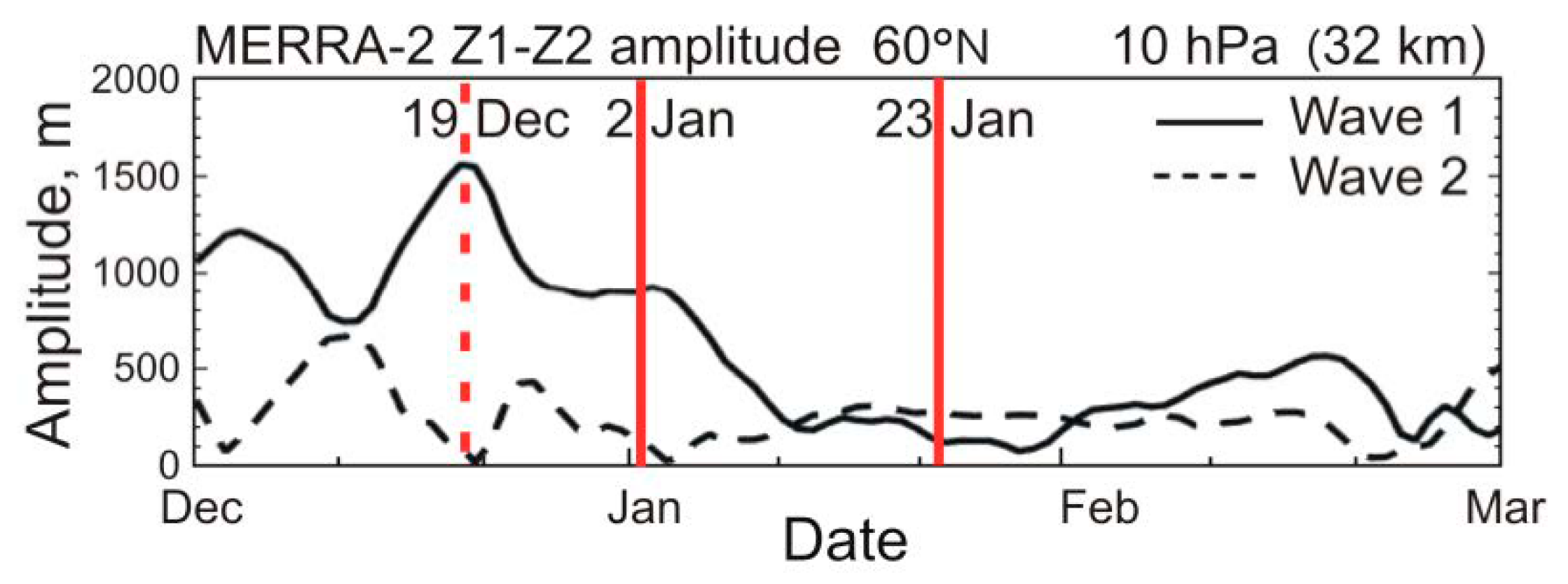
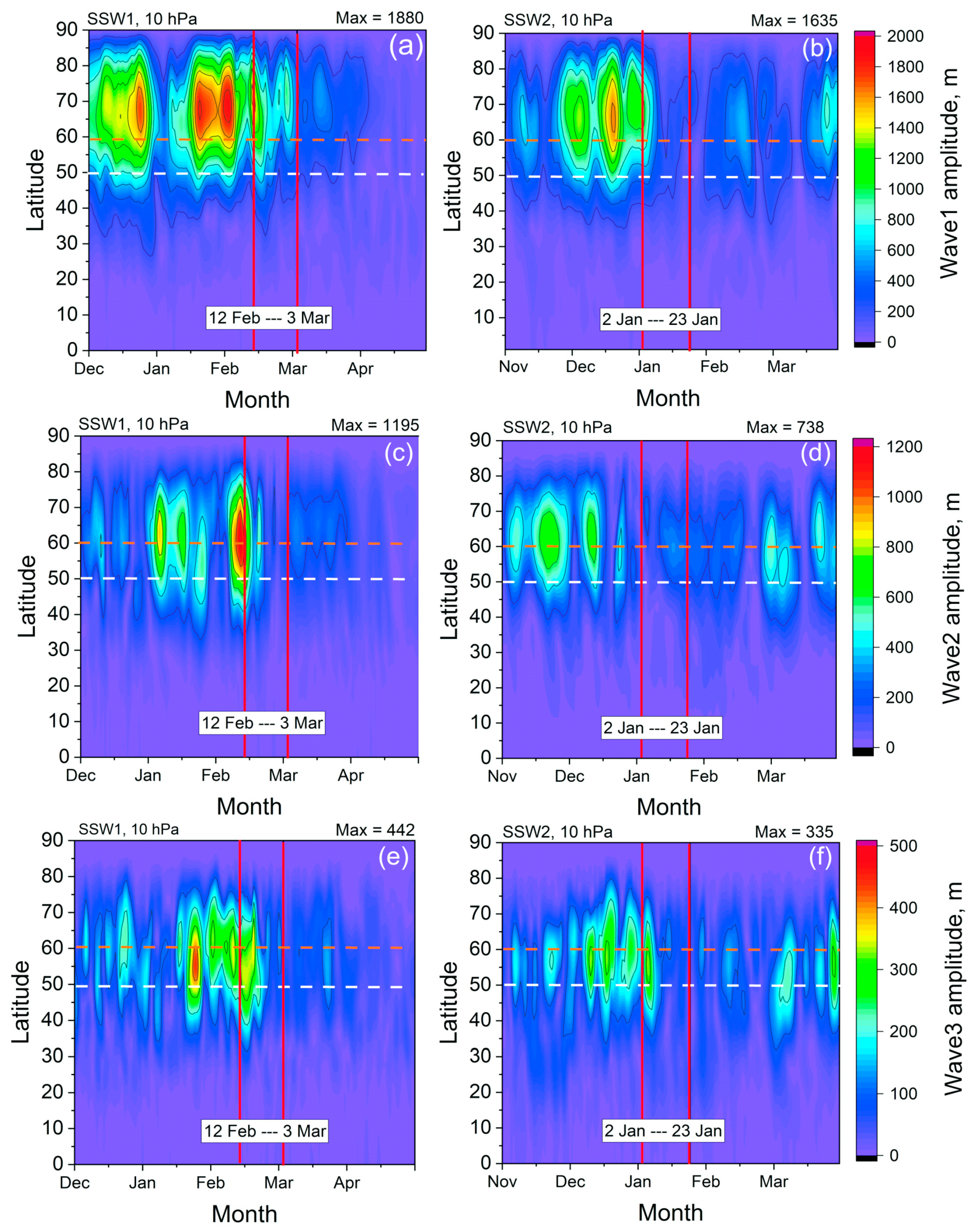
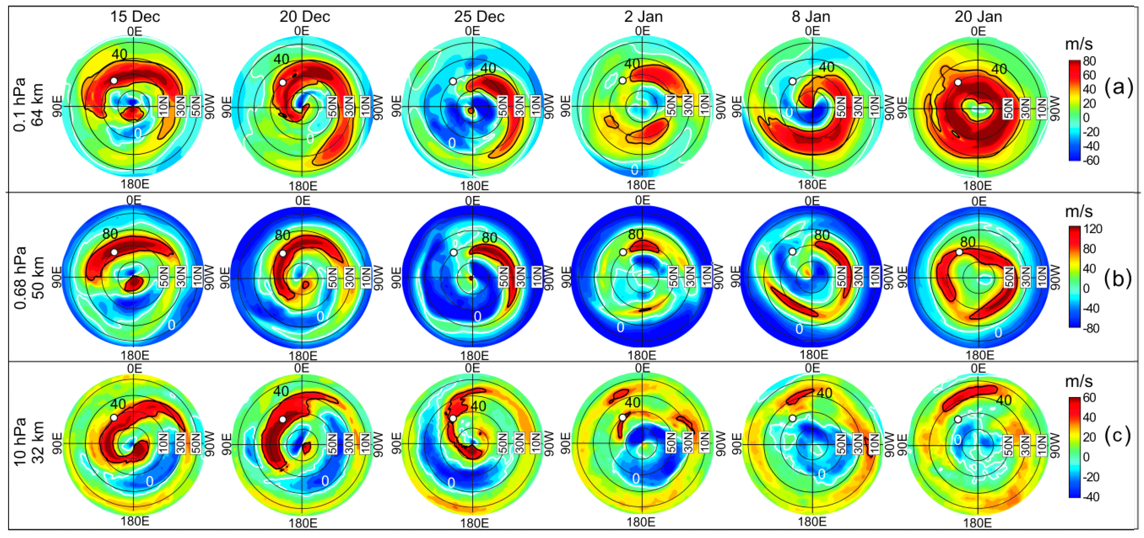
3.1. Planetary Wave Activity

A comparison of the planetary wave activity in geopotential height during the SSW1 and SSW2 events is presented in Figure 2. The planetary wave amplitudes were calculated from MERRA-2 daily mean geopotential height data at 60°N, 10 hPa, using Fourier decomposition. In the pre-warming period, the wave 1 amplitudes reached about 1700 m [26] and 1500 m (Figure 2), respectively. At the onset of SSW1, the amplitude of wave 1 decreased, and that of wave 2 increased to about 1000 m in February 2018 [26].

In early January 2019 (SSW2), the wave 1 amplitude also decreased to about 1000 m. However, the wave 2 amplitude was very small at approximately 100 m (Figure 2). Figure 1 and Figure 2 characterize the conditions of the middle stratosphere (10 hPa) at the polar vortex edge (60°N), which could affect the station region (50°N). Note that the SSW evolution occurred with (without) wave 2 amplification in the first (second) event.

In Figure 3, the latitude–time cross-sections of planetary waves 1–3 amplitudes in geopotential height at 10 hPa in NH for the winters of 2017–2018 (December–April, left) and 2018–2019 (November–March, right) are presented. The differences between the winters of 2017–2018 and 2018–2019 are very noticeable. In winter 2017–2018, all three wave components were more active and persistent than in 2018–2019 during the pre-warming time interval (Figure 3, left and right, respectively). At the same time, wave activity similarly weakened during and immediately after SSWs. This was likely caused by the easterly limitation for upward wave propagation during the SSW and the general seasonal decrease of wave activity later in spring.

There was a similar latitudinal shift of maximum amplitude between waves 1, 2, and 3 in both events: 60–80°N, 50–70°N, and 50–60°N, respectively. There was a similar latitudinal shift of maximum amplitude between waves 1, 2, and 3 in both events: 60–80°N (polar vortex region), 50–70°N (around vortex edge at 60°N, red dashed line in Figure 3), and 50–60°N (sub-vortex region), respectively.

The wave 1 and wave 2 peaks were nearly anticorrelated in time, indicating an interaction between them and the zonal flow. In the observed ‘wave 1–wave 2′ anticorrelation, wave 1 oscillations in response to ‘wave–mean flow’ interaction played a role in causing the decline of wave 2 to coincide with amplification of wave 1 due to ‘wave–wave’ interaction [52]. The anticorrelation between wave 1 and wave 2 in the stratosphere during major SSW events has been known for a long time due to observations [53] and modeling [52]. The wave 3 activity changed independently of waves 1 and 2, possibly because wave 3, on an interannual timescale, generally represents a Pacific–North America (PNA) pattern and is less associated with the annular mode [54]. The effects of wave 3, which interacted with waves 1–2, have been shown by Shi et al. [55]. The authors analyzed the modulation effects of wave 3 on wave 1–2 activity fluxes in the stratosphere during SSW in 2005. Wave 3 can enhance (weaken) the poleward wave activity, which produces conditions for upward (downward) propagation of wave 1–2 fluxes into the stratosphere. Wave 1–2 fluxes are suppressed, and wave 3 is able to enter upward into the stratosphere, causing warming to stagnate [55]. The behavior of wave 3 was closely related to the evolution of the Atlantic blocking high and the nearby structures of the temperature and pressure fields. Amplifications of wave 3 in SSW2 in Figure 3 (right) avoided those in wave 1 and wave 2, suggesting an interaction between waves 1–3.

Wave 1–3 activity in winter covered both polar and mid-latitude zones. At the MWR station latitude (50°N; white dashed line in Figure 3), the role of the higher wave number increased due to the equatorial shift of maximum amplitude noted above. Particularly, the relative contribution of wave 3 to the stratosphere disturbance at 50°N became more significant during the weakening of waves 1 and 2 (compare Figure 3e,f and Figure 3a–d, respectively, around white dashed line).

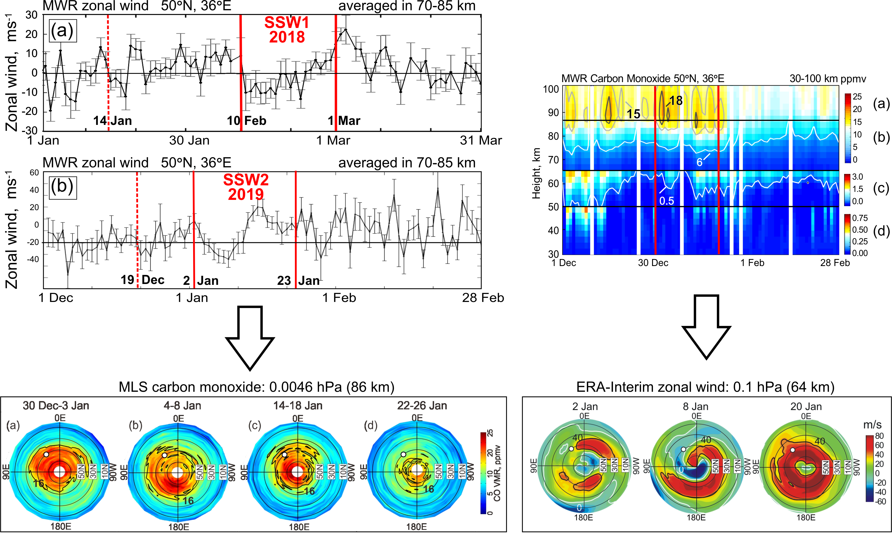
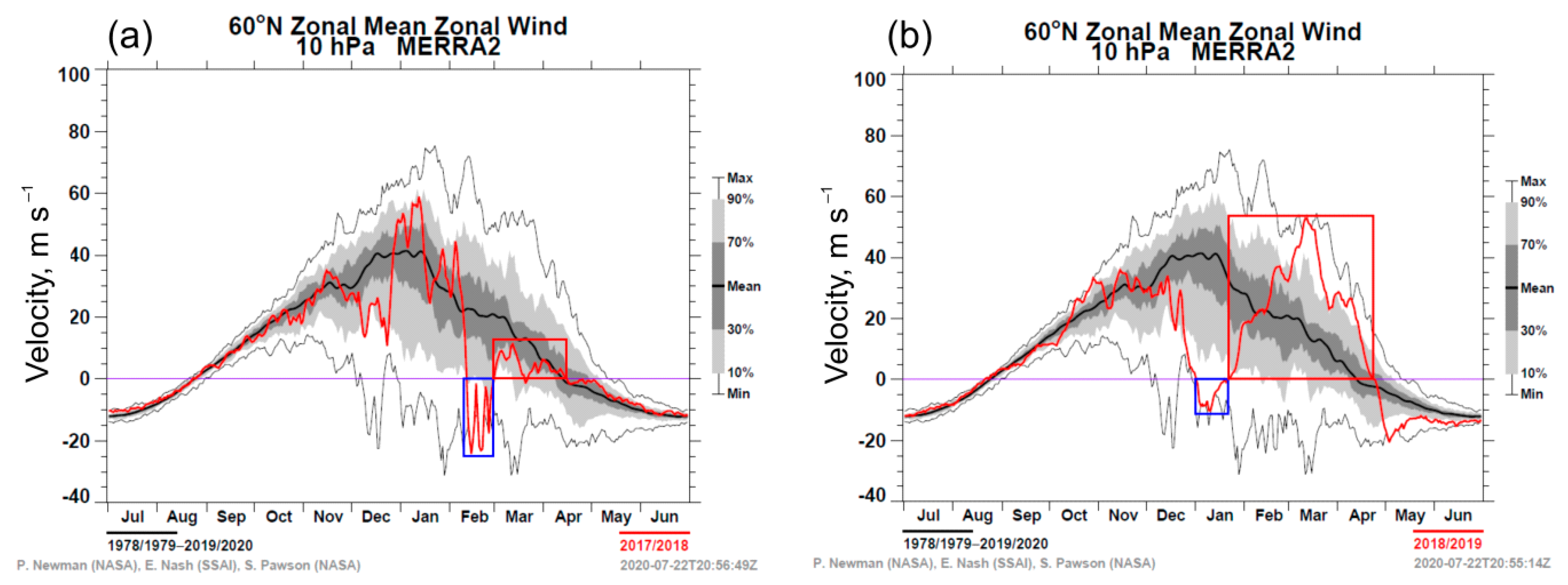
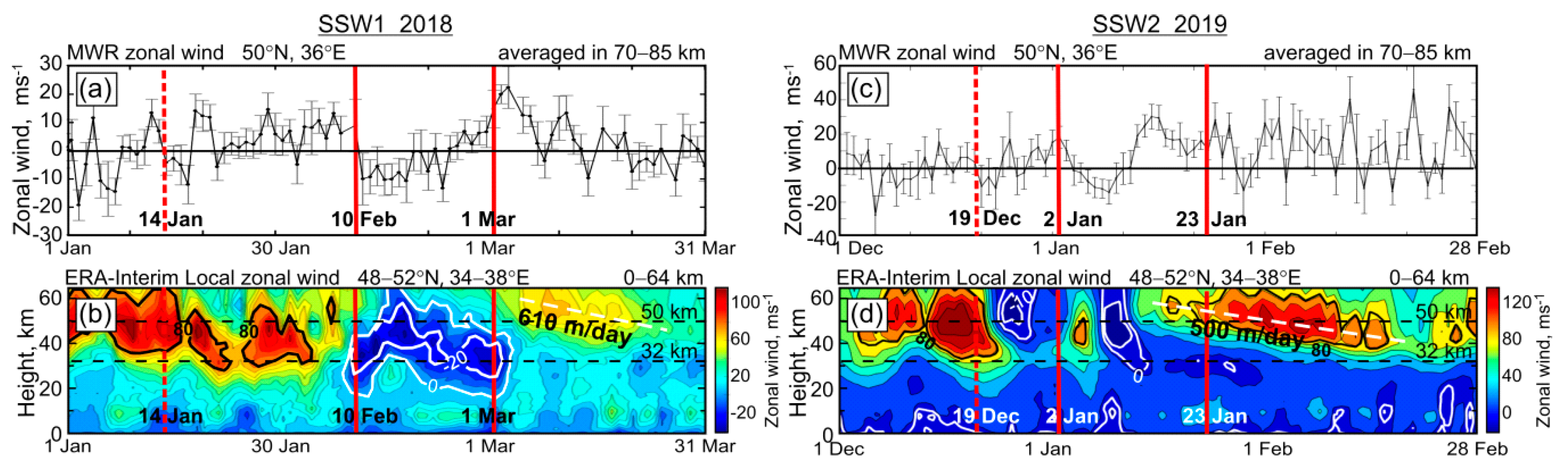
3.2. Zonal Wind Variability in the Mesosphere and Stratosphere

The MWR observations at 70–85 km over Kharkiv showed that, in SSW2, the mesospheric westerlies started to decrease (between 18 m s⁻¹ on 2 January 2019 and −12 m s⁻¹ on 7 January 2019), with reversal from westerly to easterly around 4 January (Figure 4c). For comparison, the zonal wind variations in SSW1 are reproduced in Figure 4a, based on Figure 5a of Wang et al. [26]. The westerly in SSW2 recovered after 12 January (instead of 23 January by the SSW criterion for 60°N, 10 hPa, Figure 1b) and increased to 30 m s⁻¹ on 15 January.

Both the MWR measurements and ERA-Interim data (48–52°N, 34–38°E) showed that two zonal wind reversal events over Kharkiv took place in winter 2018–2019. The event on 2 January 2019 was preceded by the event on 19 December 2018, which was locally observed between the mesosphere (Figure 4c) and upper stratosphere, where it started on 22 December 2018 (Figure 4d).

The averaged wind velocity in the mesosphere varied between +5 m s⁻¹ and −10 m s⁻¹ around 19 December 2018, according to the MWR data (Figure 4c). At the stratopause level, the change was between approximately +100 m s⁻¹ and −10 m s⁻¹ from mid- to late-December 2018, based on ERA-Interim data (Figure 4d). This reversal event did not appear from the mean zonal wind in the mid-stratosphere (at 10 hPa, 60°N, Figure 1b), providing evidence that it was a localized feature in the atmospheric circulation. Polar maps of the zonal wind from the ERA-Interim reanalysis [40] (Figure 5) may clarify how the hemispheric wind patterns affected the local observations. The white circle in Figure 5 shows the location of the MWR site Kharkiv relative to the westerly maximum outlined by the black contour. Zero wind velocity is shown by the white contour, which separates the easterly (light to dark blue) from the westerly (light green–yellow–red).

In the mid-stratosphere, a strong local westerly dominated up to mid-January, after which there was strong deceleration toward zero speed (white contour ‘0′ in mid-January at dashed horizontal line for 32 km in Figure 4d). The maps in Figure 5 show that Kharkiv was below a spiral (latitudinal-varying) structure of strong zonal wind from December 2018–early January 2019, which turned cyclonical toward the pole. This spiral-jet is a known feature and is due to planetary wave breaking, with a spiral direction due to the breaking of anticyclonic waves [56]. Due to the equatorward shift of the westerly maximum, the Kharkiv region was surrounded by near-zero zonal winds on 8 and 20 January 2019 (Figure 5c).

As noted above, the two local wind reversals appeared at the stratopause level (horizontal line at 50 km in Figure 4d). Figure 5b confirms that, due to displacements of the westerly maximum, Kharkiv was below the easterly area on 25 December 2018 and 8 January 2019. The location of Kharkiv below the easterly area in the lower mesosphere (at the 64 km level) occurred on the same dates (Figure 5a; 25 December and 8 January).

Thus, the maps for 25 December 2018 and 8 January 2019 in Figure 5a,b explain how zonal wind reversals over Kharkiv in the middle stratosphere–lower mesosphere in December and January (Figure 4d) related to the changes in horizontal wind patterns. In general, Figure 5 shows that the polar vortex structure became more fragmented below the stratopause (Figure 5c) than above the stratopause (Figure 5a). It can also be seen that the polar vortex at the stratopause and in the lower mesosphere became more much stronger between the onset and end of the SSW2 event (red to dark red between 2 and 20 January in Figure 5a,b).

The two wind reversals in the lower mesosphere (Figure 4d) occurred a few days later than in the upper mesosphere (Figure 4c), as was similarly observed during the SSW1 (Figure 4b and Figure 4a, respectively). At the Kharkiv latitudes, the wind reversal in the SSW2 did not penetrate as low into the middle stratosphere (Figure 4d) as that in SSW1 (Figure 4b). Therefore, in terms of time delay with respect to the upper mesosphere, it was impossible to compare the two events at these altitudes.

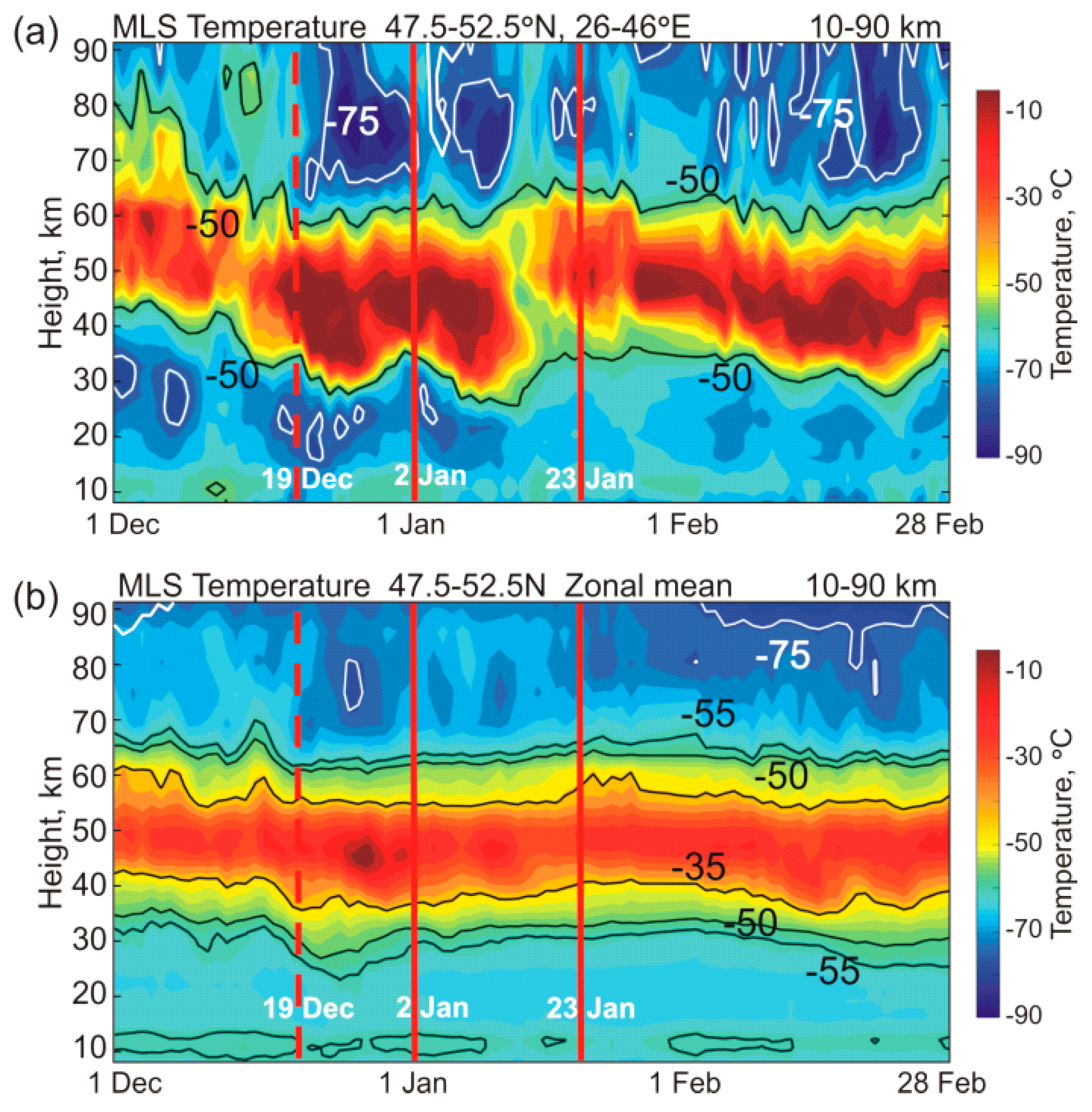
3.3. Temperature Profile Changes

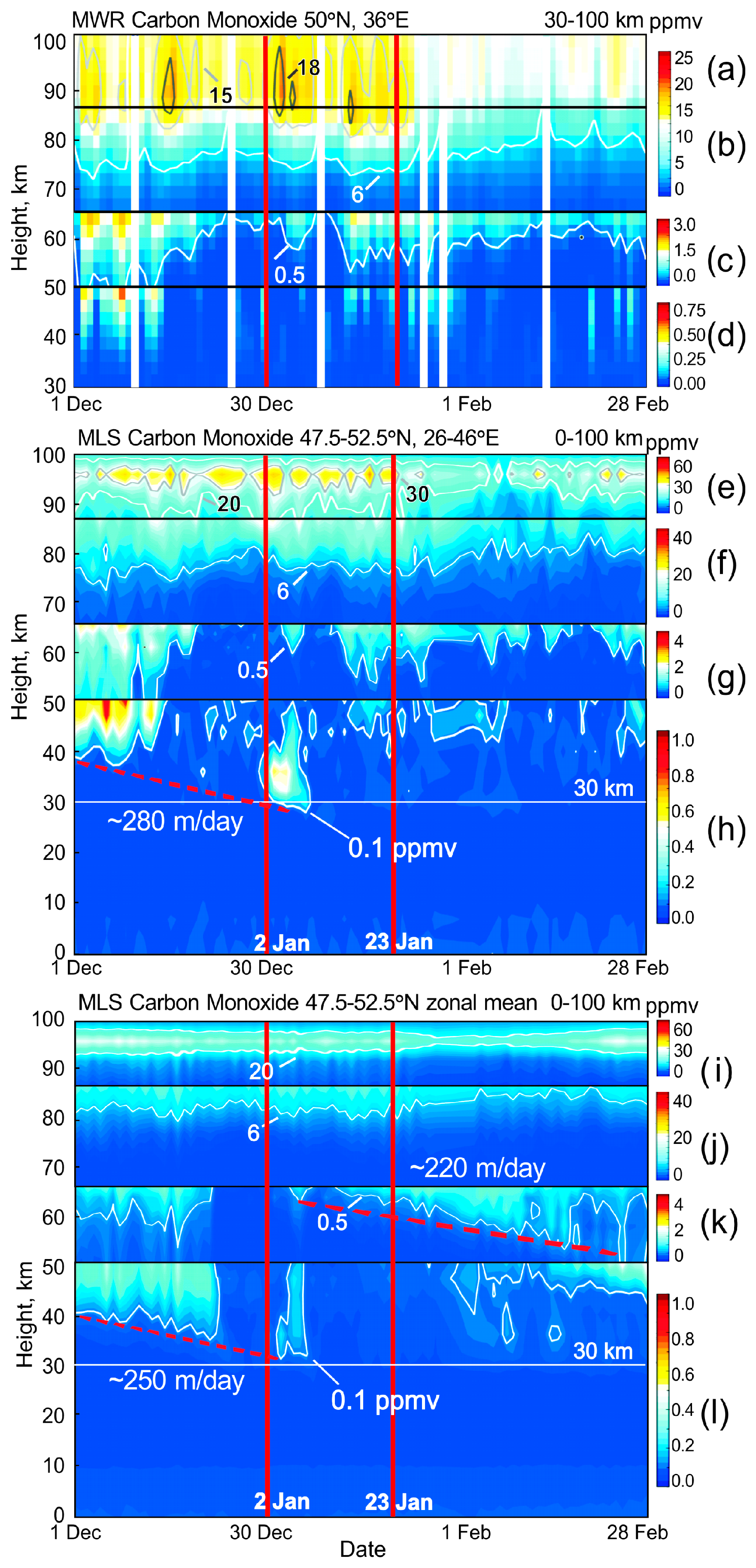
The changes in the vertical temperature profile in the Kharkiv region from the MLS measurements [42] in winter 2018–2019 (Figure 6) correspond to the changes in the zonal wave 1 activity (Figure 3b) and in the zonal circulation structure (Figure 5). Instead of the mean stratopause location at about 50 km [22], the temperature maximum was elevated to 50–60 km in the first half of December 2018 and later descended to 40–50 km until about the SSW2 end date (Figure 6a). These changes coincided with enhanced and weakened zonal wave 1 activity, respectively, in the mid-latitudes (Figure 3b) and with dominant cyclonic (westerly, 15 and 20 December 2018) and anticyclonic (easterly, 25 December 2018 and 8 January 2019) circulation over the MWR station (Figure 5a,b).

It appears that the change between the elevated and descended stratopause over the station region (Figure 6a) was influenced by the local transition from westerly to easterly due to replacement of the polar cyclone by mid-latitude anticyclone (Figure 5a,b), which, in turn, was associated with the action of zonal wave 1 (Figure 3b). Climatology has demonstrated similar anomalies in the geographical structure of polar winter stratopause temperature and height, with respect to the location of the polar vortices and anticyclones in both observations [15,16,20] and numerical modeling [17,22].

The temperature altitude–time distribution shows that the overall regional temperature in SSW2 was 10–15 °C higher (Figure 6a) than in the SSW1, as shown by Figure 6 in Wang et al. [26]. The regional temperature maximum in the stratopause region was relatively stable around the 50 km height in SSW1 but was broader (see [26]) compared to that of SSW2 (Figure 6) in both regional and zonal mean data. The downward propagation of the increased temperature anomaly between the upper and lower stratosphere observed in the first event [24] was not observed in the second event (Figure 6).

The regional stratospheric temperature in the descended stratopause region increased sharply by 15–20 °C during the SSW2 event, accompanied by a sharp decrease in the mesospheric temperature (Figure 6a), in agreement with the significant anticorrelation between mesospheric and stratospheric temperatures during SSWs (see, e.g., Siskind et al. [57]). Similar to SSW1 [26], the zonal mean temperature changes for 47.5–52.5°N in the SSW2 were not as significant and sharp (Figure 6b) as the regional ones (Figure 6a). Figure 6b confirms that the variability in the zonal means in the mid-latitude atmosphere was significantly smoothed out compared to the local and regional variability (Figure 4 and Figure 6a). The latter strongly depended on the zonal asymmetry between the polar vortex and mid-latitude anticyclones, their displacements, and possible vortex fragmentation, displaying relationships between the zonal wave 1–3 amplitudes.

3.4. CO Variability

In this section, we analyze changes in the stratosphere and mesosphere over the Kharkiv site (30–100 km; Figure 7a–c), over the Kharkiv region (47.5–52.5°N, 26–46°E, 0–100 km; Figure 7e–h), and over the latitude belt 47.5–52.5°N (Figure 7i–l). The wintertime interval from 1 December 2018 to 28 February 2019 covers the SSW2 event, including the pre- and post-warming periods.

According to the MWR data, the local CO maximum was between 90 and 100 km, with peak values of about 18 ppmv in mid-December 2018 and at the beginning of SSW2, 2–5 January 2019 (Figure 7a). The CO concentration decreased by a third between the pre-warming (~15 ppmv) and post-warming (~10 ppmv) periods. This change at the maximum of the CO layer differed from that in SSW1, in which more stable CO levels (around ~15 ppmv) were observed in winter–spring (January–March) 2018, although the CO peak at 18 ppmv was the same (Wang et al. [26], Figure 3a).

A difference also existed at the lower edge of the mesospheric CO layer, as shown by the 6 ppmv level (white curve in Figure 7b). The sharp elevation of the 6 ppmv contour (by about 8 km) observed in SSW1 [26] was completely absent in SSW2 (Figure 7b).

At the same time, a general slow increase in the height of the 6 ppmv boundary, starting at 75 km, was observed in both events. This increase was due to the seasonal trend in CO concentration between winter and summer at this altitude, as shown by Solomon et al. [27] and Lee et al. [58].

As can be seen from the CO maps near the height of the CO layer maximum (at 86 km), Kharkiv was located inside the CO-rich polar area during SSW2 (Figure 8a–c) and outside of it during the post-warming period (Figure 8d). This explains the sharp post-warming CO decrease in Figure 7a. In contrast, the Kharkiv location was in the CO-poor area at the CO layer maximum in SSW1, which resulted in the CO decrease just during the SSW1 [26].

Thus, the change in the position of the edge of the mesospheric polar vortex—which bounds the high-CO area—relative to the ground-based instrument may play a more important role in modulation of the observed CO level than the general evolution of the SSW itself.

The 0.5 ppmv level in SSW2 varied over the same altitude range of 50–65 km, but was several kilometres higher in mean altitude (Figure 7c) than that in SSW1 [26]. At the stratopause level around 50 km, a lower (higher) CO amount was observed in the first (second) half of January 2019 (Figure 7d), again determined by the Kharkiv location being outside (inside) the CO-rich area (Figure 8i–l).

Regionally averaged MLS CO data showed a post-warming CO decrease by about 10 ppmv, which is generally consistent with the local MWR data (Figure 7a) described above. The 6 ppmv and 0.5 ppmv levels also demonstrated very close variability in the local MWR data (white curves in Figure 7b,c) and the regional MLS data (white curves in Figure 7f,g). The changes in stratospheric CO during the beginning of SSW2 were unexpectedly different in the two data types (Figure 7d,h, respectively). The satellite data for the Kharkiv region in the first half of January showed the presence of mesospheric CO levels up to 0.4–0.6 ppmv in the middle–upper stratosphere (30–50 km, Figure 7h). A similar CO increase to 0.1–0.2 ppmv in the stratosphere was seen in the zonal mean MLS data (Figure 7l).

The difference between the MWR and MLS data can be explained by a small fragment of CO-rich air near Kharkiv (Figure 8n). This fragment did not appear in the local MWR record (Figure 7d), but it was partially covered by the regional MLS data (Figure 7h) averaged over a 5-degree latitudinal zone (47.5–52.5°N) and a 20-degree longitudinal sector (26–46°E), as well as by zonal mean data (Figure 7l). Generally, local and regional CO variability from MWR and MLS observations (Figure 4c, Figure 7a–h and Figure 8) is consistent with change in the polar vortex structure seen from the ERA-Interim reanalysis (Figure 5).

Zonal mean MLS data showed an even sharper mesospheric CO maximum (near 97 km, Figure 7i) than local MWR and regional MLS data (Figure 7a,e, respectively). In addition, zonal means revealed the downward motion of increased CO amount in the lower mesosphere and stratosphere (red dashed lines in Figure 7k,l) with velocities of about 220–250 m day⁻¹ (~280 m day⁻¹ from the regional MLS data in Figure 7h). These estimates are in agreement with the results for the pre-warming period of SSW1 ([26], Figure 3), in which descent tendency in the post-warming period has not been identified. The red dashed lines in Figure 7k,l show that CO-rich mesospheric air took about 2 months to penetrate from the lower mesosphere (~60 km) into the upper stratosphere (~40 km) by crossing the stratopause (~50 km). From ERA-Interim data for the Kharkiv region, the somewhat higher velocity of 500 m day⁻¹ was observed in the post-warming descent of the zonal wind maximum in the same altitude range (white dashed line in Figure 4d).

4. Discussion

In Section 3, it was shown that local zonal wind, air temperature, and the CO amount observed above the ground-based station during a SSW are dependent on the evolution of the large-scale circulation influenced by planetary wave activity. The SSW and post-SSW effects in the stratosphere and mesosphere are largely determined by the pre-warming vortex state and wave activity [8,9,39,59].

4.1. Zonal Waves, Zonal Wind, and Temperature

The stronger pre-warming wave activity in SSW1 (Figure 3) caused more complete destruction of the vortex, without significant following recovery (Figure 1a), in contrast to SSW2 (Figure 1b). In addition, SSW1 occurred in February, when the polar vortex tends to weaken seasonally (black curve in Figure 1). The timing of SSW2 occurred in January—a month and a half earlier—when minimal solar radiation was reaching the Arctic, allowing for enhanced radiative cooling in the polar region and a post-warming transition to a strong vortex [39]. The westerly zonal wind at 10 hPa, 60° N in March 2019 reached 40–50 m s⁻¹ (Figure 1b; Lee and Butler [39]). These conditions were favorable for tropospheric planetary wave propagation into the stratosphere, as confirmed by the increase of wave 1–3 amplitudes in March 2019 (Figure 3b,d,f). Similar wave amplification did not appear in the post-SSW1 period in March 2018 (Figure 3a,c,e) because of a much weaker westerly zonal wind of 5–10 m s⁻¹ (Figure 1a).

The advantages of our results are the detailed identification and comparison of SSW1 and SSW2 in terms of the locally observed changes in relation to variability in the large-scale circulation structures compared in other works [8,9,39]. As shown in Section 3.2 and Section 3.4, local mid-latitude measurements of the mesospheric wind and CO were strongly influenced by the location of the polar vortex and mid-latitude anticyclone, as well as their fragments, relative to the MWR station. A similar dependence was found in the local and regional stratopause temperature and height (Section 3.3).

Strong anticyclonic circulation adverts polar vortex air toward the equator, causing zonal asymmetries in temperature and chemical conditions in polar and mid-latitude zones due to zonal wave 1 dominance [60]. The polar maps in Figure 5 show the variable roles of cyclonic (westerly, red) and anticyclonic (easterly, blue) zonal circulation over the station (white circle) in the locally observed variations of the zonal wind velocity (Figure 4c). Note that small, well-defined fragments of vortex and anticyclone remnants, which usually exist after an SSW [16], appeared in the onset of SSW2 (2 January 2019 in Figure 5), when wind reversal started (Figure 4c). They disappeared with the polar vortex recovery at the stratopause and in the lower mesosphere (20 January in Figure 5a,b).

The stratopause temperature (height) over the Kharkiv region in the pre-warming period was lower (higher) than that during SSW2 (Figure 6a), due to the transition from westerly (in cyclonic circulation) to easterly (in anticyclonic circulation (Figure 5)). This is consistent with climatology, which has demonstrated similar differences in winter stratopause temperatures and heights with respect to the location of the polar vortices and anticyclones [22], as well as with case study results [16], composite event analysis [15], and model data [23,31].

In general, the differences between SSW1 and SSW2, in terms of local and regional wind and temperature over the MWR station at Kharkiv, were largely determined by causal relationships between the locations of the polar vortex, the mid-latitude anticyclone, and the fragments formed under planetary wave influence during the individual event.

4.2. Descent of the Mid-Latitude CO Anomalies

Due to the sharp meridional CO gradient at the polar vortex edge in winter, zonal asymmetry of the vortex accompanied by latitudinal displacements due to wave effects should dramatically affect local CO densities [27]. When comparing close dates, one can see that the CO-rich areas in Figure 8 are located poleward of the vortex edge outlined by black contours for zonal wind maximum in Figure 5 (i.e., inside the polar vortex). As in SSW1 [26], the vortex asymmetry, deformation, and fragmentation in the mesosphere led to appearance of high polar CO levels in the mid-latitudes of 30–50°N (see contours of 16 ppmv in Figure 8a–d and of 6 ppmv in Figure 8e–h).

The CO descent occurred mainly through the core of the highly displaced vortex, accompanied by an intrusion of CO-rich air from the mesosphere into the mid-stratosphere, which appears to be a defining signature of winters with major SSWs [31]. The mesospheric intrusions resulted in the increase of CO levels to 0.1–0.4 ppmv in the mid-latitude stratosphere around 50°N (30–50 km; Figure 7h,l for regional and zonal mean data, respectively). It is worth noting that the typical CO level in the mid-latitude stratosphere in winter is about 0.01–0.02 ppmv [27,29,30,61]. It should also be noted that the typical lifetime of CO in the stratosphere is about 10–20 days [28] and may be about 1 week in the presence of sunlight [27]. In the mesosphere, its lifetime is about 2 months, and in regions of total darkness, it is extremely long, and CO is approximately conserved [28]. As the SSWs in 2018 and 2019 evolved near the minimum in the 11-year solar activity change between cycles 24 and 25 (see, e.g., in [62]), the influence of solar irradiance on the CO lifetime [58] did not differ in the two events.

Due to its relatively low lifetime in the stratosphere, the increased CO amount in December and early January (Figure 7h,l) was continuously maintained by downward CO transport from the mesosphere. As noted in Section 1, the descent of CO from the mesosphere to the stratosphere induced by planetary wave activity may occur as low as 25–30 km [16,26,27,28,29,30,31].

The CO descent velocities in SSW2 (220–280 m day⁻¹ (Figure 7h,k,l)) are consistent with those observed in SSW1 with MWR at Kharkiv by Wang et al. [26] and in previous SSW events from ground-based and satellite measurements [30,59,63,64]. The CO-rich air was concentrated more uniformly inside the polar vortex region in the mesosphere (Figure 8a–h), was very heterogeneously distributed in relatively small areas at the stratopause level (Figure 8i–l) and was present only in small fragments in the stratosphere (Figure 8m–p). Therefore, registration of the CO descent in the stratosphere by local, regional, or zonal mean data depends on whether these fragments fall into the field of view of the ground-based instrument or into a certain longitudinal sector and latitudinal zone when satellite data are used. The results of Figure 8m–p and those presented in Figure 4m–p by Wang et al. [26] provide evidence that intrusions of the CO-rich air from the mesosphere into the stratosphere occur in spatially limited areas in high- and mid-latitude zones.

The 6 ppmv level in the mesosphere, on the contrary, showed a steady rise in altitude (between about 70 km and 85 km (Figure 7b,f,j, Wang et al. [26], Figure 3)). As the CO-rich air at these altitudes was replaced by CO-poor air (seen also in Figure 8a–h), a gradual decrease in the CO level took place during December–February (January–March in Wang et al. [26]). This tendency was consistent with the seasonal decrease in mesospheric CO level between winter and summer [27,58].

5. Conclusions

MWR measurements over Kharkiv, Ukraine (50.0°N, 36.3°E), located geographically in the mid-latitude region of the Eastern Europe, were presented in this paper. The local and regional manifestations of the stratospheric warming event in January 2019 (SSW2) were compared with those occurring in February 2018 (SSW1; [26]). The comparison was based on both original data from local MWR records and regional and zonal mean data from reanalyses and Aura MLS measurements. These results have advantages over earlier studies, presenting a detailed identification of the origins of the locally observed anomalies. This was achieved through analysis of the large-scale structure migration over the station, which occurred due to the interaction of the polar vortex with the mid-latitude anticyclone and could be seen from the zonal wind pattern in the ERA-Interim reanalysis data. The characteristic changes and distinctions in the mesosphere, stratosphere, and at the stratopause level between the pre- and post-warming periods (including the SSW events) were established.

The local variability of CO was explained by zonal and meridional migrations of the CO-rich polar vortex air mass, accompanied by changes in vortex asymmetry, deformation, and fragmentation. Fragments of the vortex or sub-vortex area, which appeared over Kharkiv during the SSW evolution, determined the CO levels recorded by MWR and MLS. Different locations of the vortex edge relative to the Kharkiv location resulted in the main difference between the major SSW1 and SSW2 events in terms of CO change in the pre-warming, warming, and post-warming periods. During the main phase of the SSW2 event, the CO layer maximum within the polar vortex was located over Kharkiv (Figure 8a–c) and moved away in the post-warming period. This explained the sharp post-warming CO decrease observed for this event (Figure 8d), unlike the situation for SSW1, during which Kharkiv was generally located outside the vortex edge at the time of the warming. A general slow increase in the height of the lower edge of the CO layer (at the 6 ppmv level), starting at 75 km, was observed during both events. This increase was consistent with the seasonal trend in CO concentration between winter and summer at this altitude, as shown earlier by Solomon et al. [27] and Lee et al. [58].

Fewer and fewer fragments of CO-rich air appear with decreasing height between the mesosphere and stratosphere. Therefore, changing the position of the polar vortex, which is unevenly filled with CO, affects whether the descent of CO in such fragments into the stratosphere will be observed by a ground-based instrument. The results of this work and those of Wang et al. [26] provide evidence that mesospheric intrusions of CO-rich air into the stratosphere in the major SSW1 and SSW2 events occurred only in spatially limited areas in the high- and mid-latitudes.

The mesospheric CO evolution in the major SSW1 and SSW2 events was broadly consistent between the MWR and MLS data. This was due to the more uniform filling of the CO vortex and the lesser effect of vortex fragmentation on local observation compared to the stratospheric CO.

In addition, we note that, due to the reduction in the 11-year solar activity between cycles 24 and 25, the change in solar irradiance did not cause a significant difference in the CO lifetime between the major SSW events in 2018 and 2019.

It was shown that: (i) The larger zonal wave 1–3 amplitudes before SSW1 were followed by a weaker polar vortex recovery than that after SSW2; (ii) the strong vortex recovery after SSW2 was supported by earlier event timing (midwinter); [39]; (iii) vortex strengthening after SSW2 was accompanied by wave 1–3 amplification in March 2019 (Figure 3b,d,f), which did not occur after SSW1 (Figure 3a,c,e); and (iv) the differences between SSW1 and SSW2, in terms of variability in zonal wind, temperature, and CO in the stratosphere and mesosphere, were clearly defined by the polar vortex (westerly in cyclonic circulation) and mid-latitude anticyclone (easterly) which migrated over the station (Figure 5 and Figure 8).

These results demonstrate that the large-scale circulation structures formed during the individual SSW events under the influence of planetary waves may play a major role in the locally observed variability in zonal wind, air temperature, and trace gases.

References

1. Matsuno, T. A dynamical model of the stratospheric sudden warming. J. Atmos. Sci. 1971, 28, 1479–1494. [Google Scholar] [CrossRef]
2. Butler, A.H.; Gerber, E.P. Optimizing the definition of a Sudden Stratospheric Warming. J. Clim. 2018, 31, 2337–2344. [Google Scholar] [CrossRef]
3. Vargin, P.N.; Volodin, E.M.; Karpechko, A.Y.; Pogoreltsev, A.I. Stratosphere-troposphere interactions. Her. Russ. Acad. Sci. 2015, 85, 56–65. [Google Scholar] [CrossRef]
4. Maury, P.; Claud, C.; Manzini, E.; Hauchecorne, A.; Keckhut, P. Characteristics of stratospheric warming events during Northern winter. J. Geophys. Res. Atmos. 2016, 121, 5368–5380. [Google Scholar] [CrossRef] [Green Version]
5. Charlton, A.J.; Polvani, L.M. A new look at stratospheric sudden warmings. Part I: Climatology and modeling benchmarks. J. Clim. 2007, 20, 449–469. [Google Scholar] [CrossRef]
6. Butler, A.H.; Sjoberg, J.P.; Seidel, D.J.; Rosenlof, K.H. A sudden stratospheric warming compendium. Earth Syst. Sci. Data 2017, 9, 63–76. [Google Scholar] [CrossRef] [Green Version]
7. Kruger, K.; Naujokat, B.; Labitzke, K. The unusual midwinter warming in the Southern Hemisphere stratosphere 2002: A comparison to northern hemisphere phenomena. J. Atmos. Sci. 2005, 62, 603–613. [Google Scholar] [CrossRef]
8. Butler, A.H.; Lawrence, Z.D.; Lee, S.H.; Lillo, S.P.; Long, C.S. Differences between the 2018 and 2019 stratospheric polar vortex split events. Q. J. R. Meteorol. Soc. 2020, 1–19. [Google Scholar] [CrossRef]
9. Ma, Z.; Gong, Y.; Zhang, S.D.; Luo, J.H.; Zhou, Q.H.; Huang, C.M.; Huang, K.M. Comparison of stratospheric evolution during the major sudden stratospheric warming events in 2018 and 2019. Earth Planet. Phys. 2020, 4, 493–503. [Google Scholar] [CrossRef]
10. Vargin, P.N.; Luk’yanov, A.N.; Kiryushov, B.M. Dynamic processes in the Arctic stratosphere in the winter of 2018/2019. Russ. Meteorol. Hydrol. 2020, 45, 387–397. [Google Scholar] [CrossRef]
11. WMO (World Meteorological Organization); Commission for Atmospheric Sciences. Abridged Final Report of the Seventh Session, Manila, 27 February–10 March 1978, WMO—No. 509; Secretariat of the World Meteorological Organization: Geneva, Switzerland, 1978; p. 113. [Google Scholar]
12. Manney, G.L.; Lawrence, Z.D.; Santee, M.L.; Read, W.G.; Livesey, N.J.; Lambert, A.; Froidevaux, L.; Pumphrey, H.C.; Schwartz, M.J. A minor sudden stratospheric warming with a major impact: Transport and polar processing in the 2014/2015 Arctic winter. Geophys. Res. Lett. 2015, 42, 7808–7816. [Google Scholar] [CrossRef]
13. Charlton-Perez, A.J.; Baldwin, M.P.; Birner, T.; Black, R.X.; Butler, A.H.; Calvo, N.; Davis, N.A.; Gerber, E.P.; Gillett, N.; Hardiman, S.; et al. On the lack of stratospheric dynamical variability in low-top versions of the CMIP5 models. J. Geophys. Res. Atmos. 2013, 118, 2494–2505. [Google Scholar] [CrossRef]
14. Hoffmann, C.G.; Raffalski, U.; Palm, M.; Funke, B.; Golchert, S.H.W.; Hochschild, G.; Notholt, J. Observation of strato-mesospheric CO above Kiruna with ground-based microwave radiometry–retrieval and satellite comparison. Atmos. Meas. Tech. 2011, 4, 2389–2408. [Google Scholar] [CrossRef]
15. Stray, N.H.; Orsolini, Y.J.; Espy, P.J.; Limpasuvan, V.; Hibbins, R.E. Observations of planetary waves in the mesosphere–lower thermosphere during stratospheric warming events. Atmos. Chem. Phys. 2015, 15, 4997–5005. [Google Scholar] [CrossRef] [Green Version]
16. Manney, G.L.; Schwartz, M.J.; Krüger, K.; Santee, M.L.; Pawson, S.; Lee, J.N.; Daffer, W.H.; Fuller, R.A.; Livesey, N.J. Aura Microwave Limb Sounder observations of dynamics and transport during the record-breaking 2009 Arctic stratospheric major warming. Geophys. Res. Lett. 2009, 36, L12815. [Google Scholar] [CrossRef] [Green Version]
17. Chandran, A.; Collins, R.L.; Garcia, R.R.; Marsh, D.R.; Harvey, V.L.; Yue, J.; de la Torre, L. A climatology of elevated stratopause events in the whole atmosphere community climate model. J. Geophys. Res. Atmos. 2013, 118, 1234–1246. [Google Scholar] [CrossRef]
18. Limpasuvan, V.; Orsolini, Y.J.; Chandran, A.; Garcia, R.R.; Smith, A.K. On the composite response of the MLT to major sudden stratospheric warming events with elevated stratopause. J. Geophys. Res. Atmos. 2016, 121, 4518–4537. [Google Scholar] [CrossRef] [Green Version]
19. Shepherd, M.G.; Beagley, S.R.; Fomichev, V.I. Stratospheric warming influence on the mesosphere/lower thermosphere as seen by the extended CMAM. Ann. Geophys. 2014, 32, 589–608. [Google Scholar] [CrossRef] [Green Version]
20. Zülicke, C.; Becker, E.; Matthias, V.; Peters, D.H.W.; Schmidt, H.; Liu, H.-L.; de la Torre Ramos, L.; Mitchell, D.M. Coupling of stratospheric warmings with mesospheric coolings in observations and simulations. J. Clim. 2018, 31, 1107–1133. [Google Scholar] [CrossRef]
21. Tomikawa, Y.; Sato, K.; Watanabe, S.; Kawatani, Y.; Miyazaki, K.; Takahashi, M. Growth of planetary waves and the formation of an elevated stratopause after a major stratospheric sudden warming in a T213L256 GCM. J. Geophys. Res. 2012, 117, D16101. [Google Scholar] [CrossRef]
22. France, J.A.; Harvey, V.L. A climatology of the stratopause in WACCM and the zonally asymmetric elevated stratopause. J. Geophys. Res. Atmos. 2013, 118, 2241–2254. [Google Scholar] [CrossRef]
23. Chandran, A.; Collins, R.L.; Garcia, R.R.; Marsh, D.R. A case study of an elevated stratopause generated in the Whole Atmosphere Community Climate Model. Geophys. Res. Lett. 2011, 38, L08804. [Google Scholar] [CrossRef] [Green Version]
24. Zülicke, C.; Becker, E. The structure of the mesosphere during sudden stratospheric warmings in a global circulation model. J. Geophys. Res. Atmos. 2013, 118, 2255–2271. [Google Scholar] [CrossRef]
25. Salmi, S.M.; Verronen, P.T.; Thölix, L.; Kyrölä, E.; Backman, L.; Karpechko, A.Y.; Seppälä, A. Mesosphere-to-stratosphere descent of odd nitrogen in February–March 2009 after sudden stratospheric warming. Atmos. Chem. Phys. 2011, 11, 4645–4655. [Google Scholar] [CrossRef] [Green Version]
26. Wang, Y.; Shulga, V.; Milinevsky, G.; Patoka, A.; Evtushevsky, O.; Klekociuk, A.; Han, W.; Grytsai, A.; Shulga, D.; Myshenko, V.; et al. Winter 2018 major sudden stratospheric warming impact on midlatitude mesosphere from microwave radiometer measurements. Atmos. Chem. Phys. 2019, 19, 10303–10317. [Google Scholar] [CrossRef] [Green Version]
27. Solomon, S.; Garcia, R.R.; Olivero, J.J.; Bevilacqua, R.M.; Schwartz, P.R.; Clancy, R.T.; Muhleman, D.O. Photochemistry and transport of carbon monoxide in the middle atmosphere. J. Atmos. Sci. 1985, 42, 1072–1083. [Google Scholar] [CrossRef]
28. Minschwaner, K.; Manney, G.L.; Livesey, N.J.; Pumphrey, H.C.; Pickett, H.M.; Froidevaux, L.; Lambert, A.; Schwartz, M.J.; Bernath, P.F.; Walker, K.A.; et al. The photochemistry of carbon monoxide in the stratosphere and mesosphere evaluated from observations by the Microwave Limb Sounder on the Aura satellite. J. Geophys. Res. 2010, 115, D13303. [Google Scholar] [CrossRef] [Green Version]
29. Huret, N.; Pirre, M.; Hauchecorne, A.; Robert, C.; Catoire, V. On the vertical structure of the stratosphere at midlatitudes during the first stage of the polar vortex formation and in the polar region in the presence of a large mesospheric descent. J. Geophys. Res. 2006, 111, D06111. [Google Scholar] [CrossRef] [Green Version]
30. Funke, B.; López-Puertas, M.; García-Comas, M.; Stiller, G.P.; von Clarmann, T.; Höpfner, M.; Glatthor, N.; Grabowski, U.; Kellmann, S.; Linden, A. Carbon monoxide distributions from the upper troposphere to the mesosphere inferred from 4.7μm non-local thermal equilibrium emissions measured by MIPAS on Envisat. Atmos. Chem. Phys. 2009, 9, 2387–2411. [Google Scholar] [CrossRef] [Green Version]
31. Kvissel, O.K.; Orsolini, Y.J.; Stordal, F.; Limpasuvan, V.; Richter, J.; Marsh, D.R. Mesospheric intrusion and anomalous chemistry during and after a major stratospheric sudden warming. J. Atmos. Sol. Terr. Phys. 2012, 78–79, 116–124. [Google Scholar] [CrossRef]
32. Rüfenacht, R.; Kämpfer, N.; Murk, A. First middle-atmospheric zonal wind profile measurements with a new ground-based microwave Doppler-spectroradiometer. Atmos. Meas. Tech. 2012, 5, 2647–2659. [Google Scholar] [CrossRef] [Green Version]
33. Scheiben, D.; Straub, C.; Hocke, K.; Forkman, P.; Kämpfer, N. Observations of middle atmospheric H2O and O3 during the 2010 major sudden stratospheric warming by a network of microwave radiometers. Atmos. Chem. Phys. 2012, 12, 7753–7765. [Google Scholar] [CrossRef] [Green Version]
34. Forkman, P.; Christensen, O.M.; Eriksson, P.; Billade, B.; Vassilev, V.; Shulga, V.M. A compact receiver system for simultaneous measurements of mesospheric CO and O3. Geosci. Instrum. Method Data Syst. 2016, 5, 27–44. [Google Scholar] [CrossRef] [Green Version]
35. Rüfenacht, R.; Baumgarten, G.; Hildebrand, J.; Schranz, F.; Matthias, V.; Stober, G.; Lübken, F.-J.; Kämpfer, N. Intercomparison of middle-atmospheric wind in observations and models. Atmos. Meas. Tech. 2018, 11, 1971–1987. [Google Scholar] [CrossRef] [Green Version]
36. Piddyachiy, V.; Shulga, V.; Myshenko, V.; Korolev, A.; Antyufeyev, O.; Shulga, D.; Forkman, P. Microwave radiometer for spectral observations of mesospheric carbon monoxide at 115 GHz over Kharkiv, Ukraine. J. Infrared Millim. Terahertz Waves 2017, 38, 292–302. [Google Scholar] [CrossRef]
37. Angot, G.; Keckhut, P.; Hauchecorne, A.; Claud, C. Contribution of stratospheric warmings to temperature trends in the middle atmosphere from the lidar series obtained at Haute-Provence Observatory (44 N). J. Geophys. Res. 2012, 117, D21102. [Google Scholar] [CrossRef] [Green Version]
38. Wang, Y.; Evtushevsky, O.; Milinevsky, G.; Shulga, V.; Yukhymchuk, Y.; Han, W.; Shulga, D.; Grytsai, A. The major sudden stratospheric warming impact on mid-latitude surface weather. EPJ Web Conf. 2020, 237, 04007. [Google Scholar] [CrossRef]
39. Lee, S.H.; Butler, A.H. The 2018–2019 Arctic stratospheric polar vortex. Weather 2020, 75, 52–57. [Google Scholar] [CrossRef]
40. ERA-Interim Global Atmospheric Reanalysis. Available online: https://www.ecmwf.int/en/forecasts/datasets/archive-datasets/reanalysis-datasets/era-interim (accessed on 30 August 2020).
41. MERRA-2: Atmospheric Chemistry and Dynamics Laboratory (Code 614). Available online: https://acd-ext.gsfc.nasa.gov/Data_services/met/ann_data.html (accessed on 10 September 2020).
42. MLS: Microwave Limb Sounder EOS MLS Data Readers. Available online: https://mls.jpl.nasa.gov/data/readers.php (accessed on 30 August 2020).
43. Piddyachiy, V.I.; Shulga, V.M.; Myshenko, V.V.; Korolev, A.M.; Myshenko, A.V.; Antyufeyev, A.V.; Poladich, A.V.; Shkodin, V.I. 3-mm wave spectroradiometer for studies of atmospheric trace gases. Radiophys. Quantum Electron. 2010, 53, 326–333. [Google Scholar] [CrossRef]
44. Eriksson, P.; Jiménez, C.; Buehler, S.A. Qpack, a tool for instrument simulation and retrieval work. J. Quant. Spectrosc. Radiat. Transf. 2005, 91, 47–64. [Google Scholar] [CrossRef] [Green Version]
45. Eriksson, P.; Buehler, S.A.; Davis, C.P.; Emde, C.; Lemke, O. ARTS, the atmospheric radiative transfer simulator, version 2. J. Quant. Spectrosc. Radiat. Transf. 2011, 112, 1551–1558. [Google Scholar] [CrossRef] [Green Version]
46. Buehler, S.A.; Mendrok, J.; Eriksson, P.; Perrin, A.; Larsson, R.; Lemke, O. ARTS, the atmospheric radiative transfer simulator–version 2.2, the planetary toolbox edition. Geosci. Model Dev. 2018, 11, 1537–1556. [Google Scholar] [CrossRef] [Green Version]
47. ARTS: The Atmospheric Radiative Transfer Simulator. Available online: http://www.radiativetransfer.org/ (accessed on 1 October 2020).
48. Dee, D.P.; Uppala, S.M.; Simmons, A.J.; Berrisford, P.; Poli, P.; Kobayashi, S.; Andrae, U.; Balmaseda, M.A.; Balsamo, G.; Bauer, P.; et al. The ERA-Interim reanalysis: Configuration and performance of the data assimilation system. Q. J. R. Meteorol. Soc. 2011, 137, 553–597. [Google Scholar] [CrossRef]
49. Xu, X.; Manson, A.H.; Meek, C.E.; Chshyolkova, T.; Drummond, J.R.; Hall, C.M.; Riggin, D.M.; Hibbins, R.E. Vertical and interhemispheric links in the stratosphere-mesosphere as revealed by the day-to-day variability of Aura-MLS temperature data. Ann. Geophys. 2009, 27, 3387–3409. [Google Scholar] [CrossRef] [Green Version]
50. Pumphrey, H.C.; Filipiak, M.J.; Livesey, N.J.; Schwartz, M.J.; Boone, C.; Walker, K.A.; Bernath, P.; Ricaud, P.; Barret, B.; Clerbaux, C.; et al. Validation of middle-atmosphere carbon monoxide retrievals from the Microwave Limb Sounder on Aura. J. Geophys. Res. 2007, 112, D24S38. [Google Scholar] [CrossRef] [Green Version]
51. Livesey, N.J.; Filipiak, M.J.; Froidevaux, L.; Read, W.G.; Lambert, A.; Santee, M.L.; Jiang, J.H.; Pumphrey, H.C.; Waters, J.W.; Cofield, R.E.; et al. Validation of Aura Microwave Limb Sounder O3 and CO observations in the upper troposphere and lower stratosphere. J. Geophys. Res. 2008, 113, D15S02. [Google Scholar] [CrossRef] [Green Version]
52. Robinson, W.A. A model of the wave 1–wave 2 vacillation in the winter stratosphere. J. Atmos. Sci. 1985, 42, 2289–2304. [Google Scholar] [CrossRef] [Green Version]
53. Labitzke, K. Interannual variability of the winter stratosphere in the Northern Hemisphere. Mon. Wea. Rev. 1977, 105, 762–770. [Google Scholar] [CrossRef]
54. Teng, H.; Branstator, G. A zonal wavenumber 3 pattern of northern hemisphere wintertime planetary wave variability at high latitudes. J. Clim. 2012, 25, 6756–6769. [Google Scholar] [CrossRef]
55. Shi, C.; Xu, T.; Guo, D.; Pan, Z. Modulating effects of planetary wave 3 on a stratospheric sudden warming event in 2005. J. Atmos. Sci. 2017, 74, 1549–1559. [Google Scholar] [CrossRef]
56. Kuang, X.; Zhang, Y.; Huang, Y.; Huang, D. Spatial differences in seasonal variation of the upper-tropospheric jet stream in the Northern Hemisphere and its thermal dynamic mechanism. Theor. Appl. Climatol. 2014, 117, 103–112. [Google Scholar] [CrossRef]
57. Siskind, D.E.; Coy, L.; Espy, P. Observations of stratospheric warmings and mesospheric coolings by the TIMED SABER instrument. Geophys. Res. Lett. 2005, 32, L09804. [Google Scholar] [CrossRef] [Green Version]
58. Lee, J.N.; Wub, D.L.; Ruzmaikin, A.; Fontenla, J. Solar cycle variations in mesospheric carbon monoxide. J. Atmos. Sol. Terr. Phys. 2018, 170, 21–34. [Google Scholar] [CrossRef]
59. Orsolini, Y.J.; Limpasuvan, V.; Pérot, K.; Espy, P.; Hibbins, R.; Lossow, S.; Larsson, K.R.; Murtagh, D. Modelling the descent of nitric oxide during the elevated stratopause event of January 2013. J. Atmos. Sol. Terr. Phys. 2017, 155, 50–61. [Google Scholar] [CrossRef]
60. Harvey, V.L.; Pierce, R.B.; Hitchman, M.H. A climatology of stratospheric polar vortices and anticyclones. J. Geophys. Res. 2002, 107, 4442. [Google Scholar] [CrossRef]
61. Engel, A.; Möbius, T.; Haase, H.-P.; Bönisch, H.; Wetter, T.; Schmidt, U.; Levin, I.; Reddmann, T.; Oelhaf, H.; Wetzel, G.; et al. Observation of mesospheric air inside the arctic stratospheric polar vortex in early 2003. Atmos. Chem. Phys. 2006, 6, 267–282. [Google Scholar] [CrossRef] [Green Version]
62. Sunspot Index and Long-Term Solar Observations. Available online: http://www.sidc.be/silso/DATA/SN_m_tot_V2.0.txt (accessed on 30 August 2020).
63. McLandress, C.; Scinocca, J.F.; Shepherd, T.G.; Reader, M.C.; Manney, G.L. Dynamical control of the mesosphere by orographic and non-orographic gravity wave drag during the extended northern winters of 2006 and 2009. J. Atmos. Sci. 2013, 70, 2152–2169. [Google Scholar] [CrossRef]
64. Ryan, N.J.; Kinnison, D.E.; Garcia, R.R.; Hoffmann, C.G.; Palm, M.; Raffalski, U.; Notholt, J. Assessing the ability to derive rates of polar middle-atmospheric descent using trace gas measurements from remote sensors. Atmos. Chem. Phys. 2018, 18, 1457–1474. [Google Scholar] [CrossRef] [Green Version]
Figure 1. Mean zonal wind during the (a) 2018 and (b) 2019 sudden stratospheric warming (SSW) events at 60° N, 10 hPa by MERRA-2 data [41]. Note the difference in the easterly and westerly persistence and velocity change in the SSW and post-SSW time intervals (outlined by blue and red rectangles, respectively).
Remotesensing 12 03950 g001
Figure 2. Wave 1 and wave 2 amplitudes in geopotential height at 60°N, 10 hPa, in December 2018–February 2019 by the MERRA-2 time series data [41]. The SSW2 event is bounded by red vertical lines. The dashed red vertical line marks the beginning of zonal wind reversal from the local microwave radiometer (MWR) measurements in December 2018.
Remotesensing 12 03950 g002
Figure 3. Latitude–time cross-section of the amplitudes of planetary waves 1, 2, and 3 at 10 hPa in Northern Hemisphere (NH) for: (a,c,e) December 2017–April 2018 and (b,d,f) November 2018–March 2019 by MERRA-2 data [41]. Red vertical lines mark the SSW start and end dates. Red (white) dashed horizontal lines mark the mean vortex edge latitude of 60° N (MWR site latitude 50°N).
Remotesensing 12 03950 g003
Figure 4. Zonal wind variability in (a,b) SSW1 in January–March 2018 and (c,d) SSW2 in December 2018–February 2019 by (a,c) the MWR data averaged in the altitude range of 70–85 km; and (b,d) time–altitude sections of the ERA-Interim [40] zonal wind averaged over latitudes 48–52°N and longitudes 34–38°E (centered at the Kharkiv microwave radiometer site; 50°N, 36°E). The vertical bars in (a,c) are standard deviations that reflects the wind speed variability at daily timescale. The SSW events are bounded by red vertical lines. Dashed vertical lines in (c,d) mark the start date of zonal wind reversal in December 2018 and 2019. Dashed horizontal lines in (c,d) mark the stratopause level at ~50 km and middle stratosphere level at ~32 km. Plots (a,b) modified from Wang et al. [26], their Figure 5.
Remotesensing 12 03950 g004
Figure 5. The zonal wind field over the NH (0–90°N) on selected dates between 15 December 2018 and 20 January 2019 from the ERA-Interim reanalysis [40]: (a) At the lower mesosphere (64 km); (b) stratopause (50 km); and (c) middle stratosphere (32 km) levels before (15, 20, and 25 December 2018) and during (2, 8, and 20 January 2019) the SSW2 event. The white circle shows location of the MWR site Kharkiv relative to the westerly maximum marked by the black contours. The white contour corresponds to zero zonal wind.
Remotesensing 12 03950 g005
Figure 6. Temperature altitude profiles by Aura Microwave Limb Sounder (MLS) data [42] for SSW2 in winter 2019: (a) Over the Kharkiv region, and (b) zonal average in the band 47.5–52.5°N.
Remotesensing 12 03950 g006
Figure 7. Vertical profile variations of mesospheric carbon monoxide (CO) by MWR (Kharkiv) and MLS [42] data in the SSW2 event: (ad) Local mesospheric and stratospheric CO profiles from MWR measurements over Kharkiv in the altitude range 30–100 km; (eh) regional CO profiles from MLS measurements averaged over latitudes 47.5–52.5°N and longitudes 26–46°E centered at the Kharkiv MWR site (50°N, 36°E); and (il) CO profiles from the MLS zonal means in latitudinal band 47.5–52.5°N. Selected CO levels are highlighted by white, grey, and black contours (see text for details). Data for December 2018–February 2019 are presented and the time interval of significant variations in atmosphere parameters due to the SSW2 event from 2–23 January 2019 is bounded by red vertical lines.
Remotesensing 12 03950 g007
Figure 8. The 5-day mean CO field in the NH stratosphere/mesosphere (0–90°N, between 32 km and 86 km) from the MLS measurements [42] before (a,e,i,m), during (b,f,j,n) and (c,g,k,o), and after (d,h,l,p) the SSW2 in 2019. The white circle shows the location of the MWR Kharkiv site relative to the high and low CO content areas, which are separated by black contours. Note that Kharkiv fell under the high CO area in the mesosphere during SSW2 (b,c,f,g), which was displaced relative to Kharkiv afterward (d,h). This displacement explains the stepwise decrease in the post-warming CO level from the MWR data in Figure 7a and from regional MLS data in Figure 7e.
Remotesensing 12 03950 g008
Publisher’s Note: MDPI stays neutral with regard to jurisdictional claims in published maps and institutional affiliations.