Driven by Drones: Improving Mangrove Extent Maps Using High-Resolution Remote Sensing

Abstract

This study investigated how different remote sensing techniques can be combined to accurately monitor mangroves. In this paper, we present a framework to use drone imagery to calculate correction factors which can improve the accuracy of satellite-based mangrove extent. We focus on semi-arid dwarf mangroves of Baja California Sur, Mexico, where the mangroves tend to be stunted in height and found in small patches, as well as larger forests. Using a DJI Phantom 4 Pro, we imaged mangroves and labeled the extent by manual classification in QGIS. Using ArcGIS, we compared satellite-based mangrove extent maps from Global Mangrove Watch (GMW) in 2016 and Mexico’s national government agency (National Commission for the Knowledge and Use of Biodiversity, CONABIO) in 2015, with extent maps generated from in situ drone studies in 2018 and 2019. We found that satellite-based extent maps generally overestimated mangrove coverage compared to that of drone-based maps. To correct this overestimation, we developed a method to derive correction factors for GMW mangrove extent. These correction factors correspond to specific pixel patterns generated from a convolution analysis and mangrove coverage defined from drone imagery. We validated our model by using repeated k-fold cross-validation, producing an accuracy of 98.3% ± 2.1%. Overall, drones and satellites are complementary tools, and the rise of machine learning can help stakeholders further leverage the strengths of the two tools, to better monitor mangroves for local, national, and international management.

1. Introduction

For over 20 years, researchers have published literature on the economic and ecologic value of mangroves and their ecosystem services. From supporting local fisheries to mitigating climate change, the value of mangrove ecosystem services totals at least $50,000 USD (2007) per hectare annually [1]. Mangroves are considered an essential ocean variable—a term developed by the Global Ocean Observing System, a program born from the 1992 United Nations Conference on Environment and Development—as their extent is an indicator of tropical coastal ecosystem health [2]. The societal and ecological importance of mangroves is further highlighted in Halpern et al. [3], in which mangroves form part of three sub-goals of ten goals that make up the ocean health index. Mangroves provide fundamental societal and economic value; yet, relative to other essential ocean variables with high social impact, mangroves are currently observed and monitored at low spatial and temporal scales [4].

Mangrove-related ecosystem services such as fisheries, coastal protection, and carbon sequestration are currently calculated based on area, driving a need for robust extent maps [1]. The development of an accurate, systematic monitoring system can greatly improve our understanding of the global and local state of mangroves and facilitate effective conservation at these various scales [5]. Even though there are large advancements in technology, and monitoring methodologies are quickly developing, accurate, reliable, and timely information on the distribution of mangrove forests has yet to be attained [6,7].

To address this need, the use of remote-sensing and machine-learning technology to quickly map mangroves has been on the rise [8,9,10,11]. Efforts have largely focused on the use of satellite imagery, due to its ability to capture large areas at a time, its low cost, and the large range of sensors that satellites are equipped with [12,13]. The most recent global effort to map mangroves comes from Global Mangrove Watch (GMW), which leverages machine learning on L-band synthetic aperture radar (SAR) data and optical imagery to estimate mangrove extent for multiple years [14]. Similar national mangrove inventories have also been undertaken. For example, since 2005, in Mexico, the National Commission for the Knowledge and Use of Biodiversity (CONABIO) established a mangrove-monitoring baseline, mapping national mangrove extent every five years, using satellite imagery, machine learning, and verification by helicopter aerial surveys [15,16]. Mexico’s national-level monitoring is among the highest frequency and regularity among countries with mangroves.

Though satellite imagery is able to map the entire globe, the spatial scale of 10 m/pixel such as that of the Sentinel satellite imagery is still much coarser than the centimeters/pixel resolution of small unmanned aerial vehicles (drones), resulting in different estimations in mangrove extent (Yang et al., 2020). Even very high-resolution satellite imagery, such as WorldView-2 (5 m/pixel) and Pleiades-1B (50 cm/pixel), is outperformed by drones [13,17]. Drones’ ability to map at a fine resolution permits successful habitat identification [10,18]. Drones also have the advantage of flexibility. Drones can collect data at any given time and in very targeted areas, as compared to satellites, which must fly their set mission path [19,20]. For these reasons, drones are filling in the gap between satellite and on-the-ground surveys.

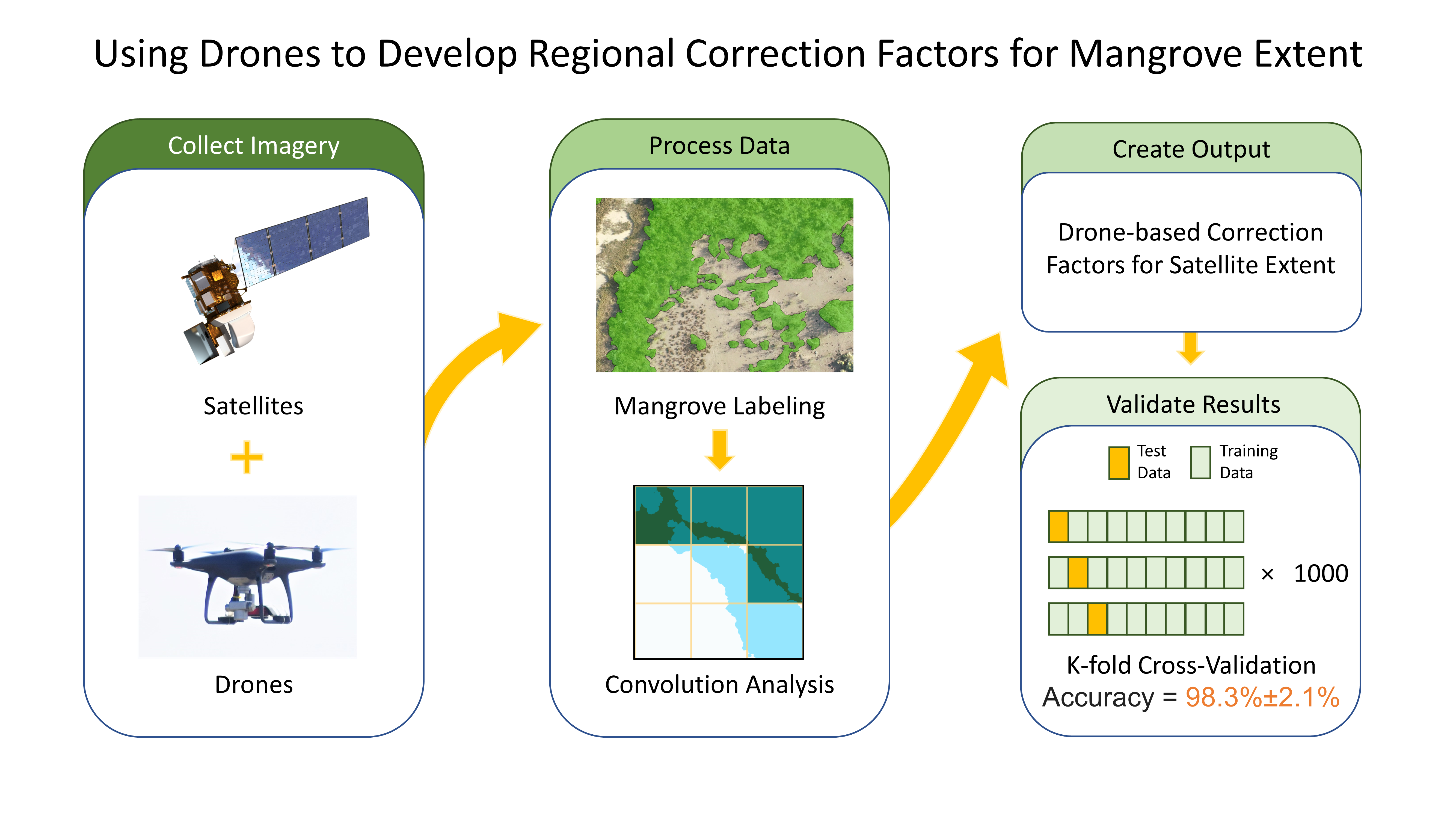
This study investigates how drones can be leveraged to correct satellite estimates of local mangrove coverage. We compared estimations of mangrove extent derived from a spectrum of remote sensing methodologies and machine learning integration. Specifically, we addressed the need to link global data with local management by contextualizing global datasets, such as GMW, to local areas [11,21]. We analyze the differences in reported mangrove extent among GMW, CONABIO, and drones and highlight patterns of overestimation that can be corrected. We present a framework for developing correction factors from drones to improve mangrove area estimations derived from satellites. By analyzing specific pixel patterns, we calculated correction factors to be applied on the GMW dataset and improved the estimation by up to 99% per raster cell in dwarf mangroves. This study ultimately reveals the importance of coupled remote sensing tools for monitoring mangrove extent. The methodology presented here can be adapted to other regions, to contextualize existing global or national datasets to local areas, and can be particularly useful in fragmented or threatened mangrove ecosystems.

2. Materials and Methods

2.1. Study Sites

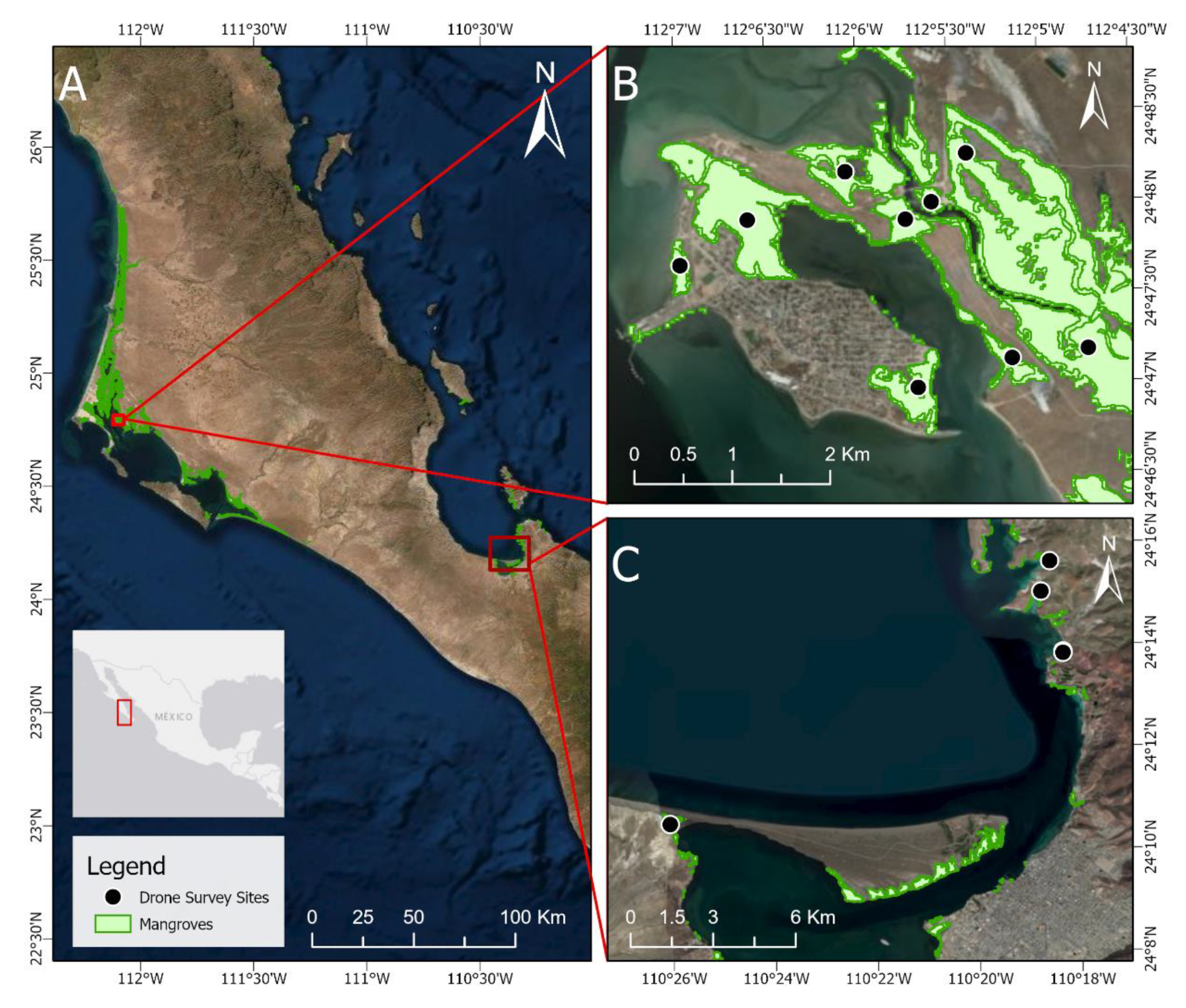
Our efforts were concentrated in two locations in Baja California Sur (BCS), Mexico: Puerto San Carlos in the Comondú Municipality and Ensenada de La Paz in the La Paz Municipality (Figure 1A). Puerto San Carlos is located within Magdalena Bay, facing the Pacific Ocean (Figure 1B), 266 km northwest from the capital city of La Paz (24°47′6.73″ N; 112°06′20.10″ W). The area maintains a semi-arid climate, with the annual average temperature oscillating between 18 and 22 °C, and the greatest contributions of fresh water are from precipitation from May to October [15,22]. The area is surrounded by rocky islands, with sand dunes and dwarf mangroves. These mangroves cover approximately 22,312 hectares in the bay and are composed of three species: Rhizophora mangle, Avicennia germinans, and Laguncularia racemosa [16,23,24].

The second sampling area is the lagoon system of Ensenada de La Paz on the southeastern coast of the Baja California Peninsula, facing the Gulf of California (Figure 1C), (24°19′17.13″ N; 24°19′17.13″ N). La Paz is also considered a semi-arid region, with an average annual temperature of 23.5 °C and a rainy season between July and October that is also the main source of fresh water to the region. The region is characterized by intertidal plains, scrub coastal plains, dunes, and low hills. These mangrove ecosystems cover a total of 9184 hectares [25,26] and are composed of the same three species as in Puerto San Carlos [27,28]. Both Puerto San Carlos and La Paz have semi-arid mangroves that are dwarfed in height (from one to seven meters) [29].

2.2. Datasets

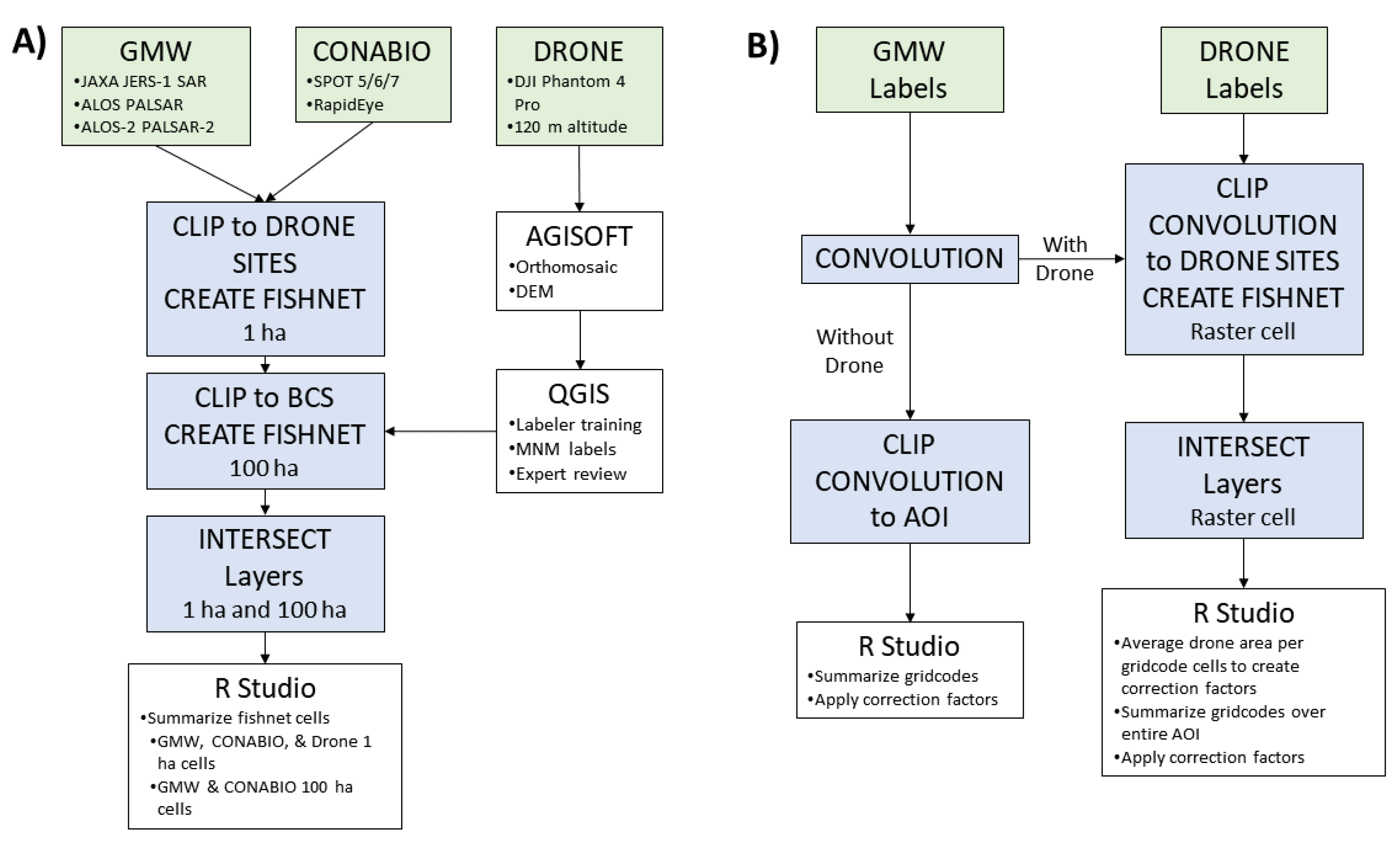
Our study used data of mangrove extent published by CONABIO in 2015 (Valderrama-Landeros et al., 2017), by GMW in 2016 (Bunting et al., 2018), and drone imagery collected from La Paz and Puerto San Carlos in BCS during May and July 2018 and July 2019 (Figure 1). GMW data have the coarsest imagery, with 25 m pixel resolution, and the mangrove classification was generated by machine learning algorithms. CONABIO data have a 10 m pixel resolution, and mangrove classification was generated from a mixture of statistical analyses and aerial verification. Drones had the highest resolution among the imagery used in this study, with a 3 cm pixel resolution and mangrove classification manually achieved. A workflow of how these datasets were processed in this study is provided in Figure 2.

2.2.1. Satellite Data

In their 2015 estimation of mangrove extent, CONABIO primarily used imagery from SPOT-5 (10 m resolution), and imagery from SPOT-6 (6 m resolution), SPOT-7 (6 m resolution), and RapidEye (5 m resolution) when SPOT-5 imagery was unavailable or of insufficient quality [26]. The spectral bands on SPOT-5 are green, red, near-IR, and SWIR, while SPOT-6, SPOT-7, and RapidEye only have visible to near-IR bands. CONABIO normalized the imagery to 10 m resolution and employed supervised and unsupervised classification schemes to map mangrove extent, using past mangrove mapping efforts as a baseline reference. These classifications were validated with aerial photos from helicopter flights in 2015 and 2016, achieving an overall accuracy of 90% to 93%.

GMW used a combination of synthetic aperture radar data from JAXA JERS-1 SAR, ALOS PALSAR, and ALOS-2 PALSAR-2, with optical image data from Landsat-5 and Landsat-7, using the blue, green, red, near-IR, SWIR1, and SWIR2 bands [14]. GMW then generated mangrove extent maps by using machine learning algorithms (Extremely Randomized Trees Classifier) trained on previous mangrove maps. Accuracy was reported at 93.6–94.5% by assessing 53,878 points across 20 global sites.

Additionally, we used 100% cloud free RapidEye 5 m resolution imagery downloaded from Planet Labs, for February 2015, to rectify the temporal differences within this paper’s methodology [30]. This imagery was used to visually inspect significant changes in mangrove extent, as compared to our drone surveys from 2018 and 2019.

2.2.2. Drone Data

In 2018 and 2019, we captured drone imagery across 14 sites in BCS, covering 455.43 ha, using the built-in camera of a DJI Phantom 4 Pro. Missions were planned by using DJI Ground Station Pro. For each site, we collected two sets of images: one at 120 m above ground level, and another at 10 m above canopy height. When needed, we conducted multiple flights at 120 m altitude, to cover the entire forest. The flights at 10 m only covered a small portion of each site and were used to verify habitat identification. Images were taken at 85% overlap in all directions. Further details of this flight method can be found in Hsu et al. [31].

We performed image orthorectification on the drone imagery, using Agisoft Photoscan version 1.4.2 or newer. Individual photos were reviewed, to exclude those with poor quality, and we removed any with severe reflections from the water. After aligning the photos, we reviewed the resulting sparse point cloud and removed obvious outlying points. Dense point clouds were then generated by using the highest quality setting, further cleaned of outliers, and then used to generate orthomosaics with a 3 cm pixel resolution.

Trained labelers applied a manual classification to the drone imagery, using QGIS version 2.18 or newer, with polygons classified into mangrove and non-mangrove categories [32]. Each labeler was extensively trained on how to identify mangroves from aerial imagery, and their labels were reviewed by mangrove experts and cross-referenced with the drone imagery taken at 10 m.

2.3. Dataset Comparison

We first compared our drone extent layer with satellite extent layers, to investigate the discrepancies among the datasets. We downloaded GMW and CONABIO data from Ocean Data Viewer by United Nations Environment Programme World Conservation Monitoring Centre [14] and CONABIO [26], respectively. We uploaded both datasets, along with our drone label dataset into ArcGIS Pro 2.4, and clipped the datasets to the extent of our drone images, before projecting into North American Albers Equal Area Conic. To compare the mangrove areas’ estimations from such different datasets and heterogeneous study area, we first subdivided our study area into standardized 1-hectare fishnet cells, and then, within each cell, we compared the percent overlap among the datasets (Figure 3). To maximize the number of samples from our limited drone dataset while maintaining the minimum area of analysis recommended by Bunting et al. (2018), we set fishnet cells to one hectare. Cells on the edges of drone imagery had areas less than one ha, as the fishnet cells were constricted to the area covered by drones.

To calculate the percent overlap among the datasets, we created additional layers of mangrove area: (i) the area of the drone and CONABIO datasets combined (union); (ii) the area of the drone and GMW combined (union); (iii) and (iv) the area where the respective datasets agree (intersection); (v) and (vi) the drone area, excluding the respective intersecting data; (vii) the CONABIO data, excluding intersecting data; and (viii) the GMW data, excluding intersecting data. We then intersected these new layers with the fishnet cells, calculated the area for each of the layers in each cell, and assigned unique IDs, to create the final dataset for statistical analyses in R. We repeated this process with just CONABIO and GMW datasets for all of BCS, to provide a reference of our analysis beyond the sites imaged by drones, setting fishnet cells at 100 ha, to reflect the greater area analyzed.

All statistical procedures were completed in R Studio (version 1.2). Using 2015 RapidEye satellite imagery from Planet Lab, we also visually identified types of habitat overestimation from CONABIO and GMW datasets.

We then investigated if the differences in mangroves’ extent between GMW and drones was caused by a systematic error or just noise from image resolution differences. We converted our mangrove label shapefiles generated from drones to a raster (WGS 1984), downsampling the imagery by using nearest neighbor to match the pixel resolution of the GMW raster. We then intersected the two datasets and used raster cell statistics to calculate the intersection over union of all pixels between the two datasets.

2.4. Correction Factor

To correct the differences between the satellite-derived mangrove area and our drone data, thereby localizing a global dataset, we generated correction factors for GMW based on a convolution analysis (Figure 2). We only defined correction factors for GMW, as the CONABIO data are restricted to Mexico, while GMW is a more widely used global dataset.

2.4.1. Convolution Analysis

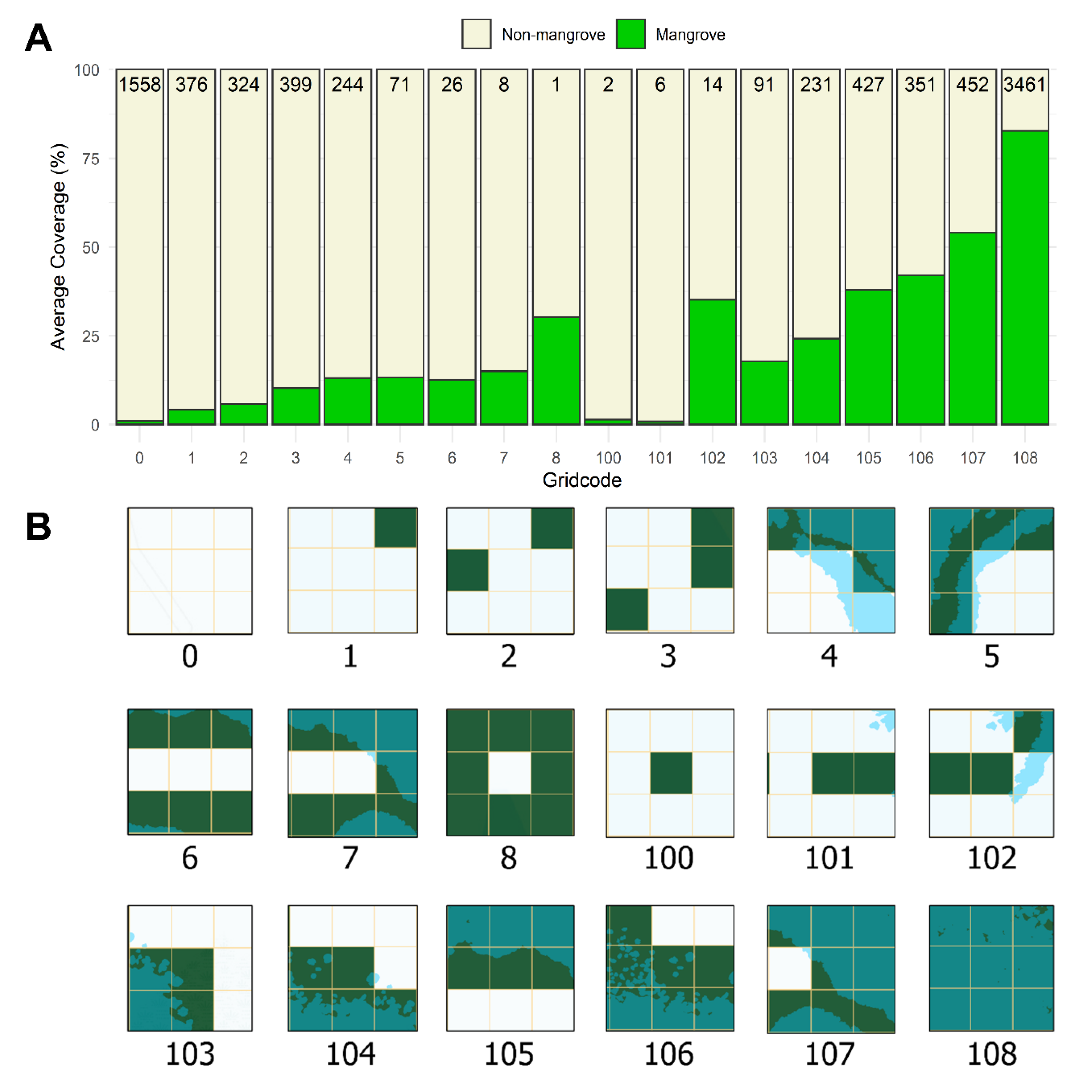
Using ArcGIS Pro, we projected the GMW 2016 raster layer and drone mangrove labels into WGS 1984. We ran the raster function “Convolution” and then clipped the GMW convolution raster to the drone sites. We defined our own 3 × 3 convolution, with a center cell value of 100 and the eight surrounding boundary cell values of one. A cell value (hereby referred to as gridcode) greater or equal to 100 represents that a GMW mangrove pixel was detected in the center cell. The ones digit of the gridcode indicated the number of adjacent cells that detect mangrove. From our convolution, there are a total of 18 different gridcodes, from 0 to 8 (non-mangrove center cell) and from 100 to 108 (mangrove center cell).

2.4.2. Gridcode Analysis

We then intersected the following layers: the GMW raster with gridcodes, a fishnet (a shapefile with cells the same size as a GMW raster cell), and the drone labels. Each fishnet cell was given a unique ID. Next, we projected the resulting layer to Albers North America Equal Area Conic and calculated the area of each cell. Because the GMW raster is limited to the drone imagery, for this specific analysis, we analyzed cells that captured at least 99% of the fishnet area with both the GMW and drone labels. We then calculated mangrove and non-mangrove coverage of each individual raster cell and computed the average percent of mangrove coverage for each gridcode. To use this average as a correction factor for GMW mangrove extent, the following formula was implemented for each gridcode:

$$\begin{gathered} \mathrm{Mangrove}\mathrm{Area}=\mathrm{Average}\mathrm{mangrove}\mathrm{cover}(\%)\times \mathrm{Cell}\mathrm{count}\mathrm{of}\mathrm{gridcode} \\ \times \mathrm{raster}\mathrm{cell}\mathrm{area} \end{gathered}$$

(1)

2.4.3. Validation

We validated this methodology in two ways. First, we summed the area by using the formula above for all gridcodes, and then compared it with the total mangrove area detected by the drone. Second, we conducted a repeated k-fold cross-validation. We set k equal to 10 and repeated the k-fold cross validation 1000 times, as each run splits the data differently [33]. The error of the model was measured to be 1.7% ± 2.1% (SD). We define the error as the mean absolute difference between the estimated and hand-labeled mangrove extent. Finally, we performed the same convolution analysis to generate gridcodes for all the mangroves in BCS and applied the correction factors calculated above, to improve area estimation. We compared our corrected results with the area reported by GMW and CONABIO for the whole BCS state.

3. Results

3.1. Drone Validation

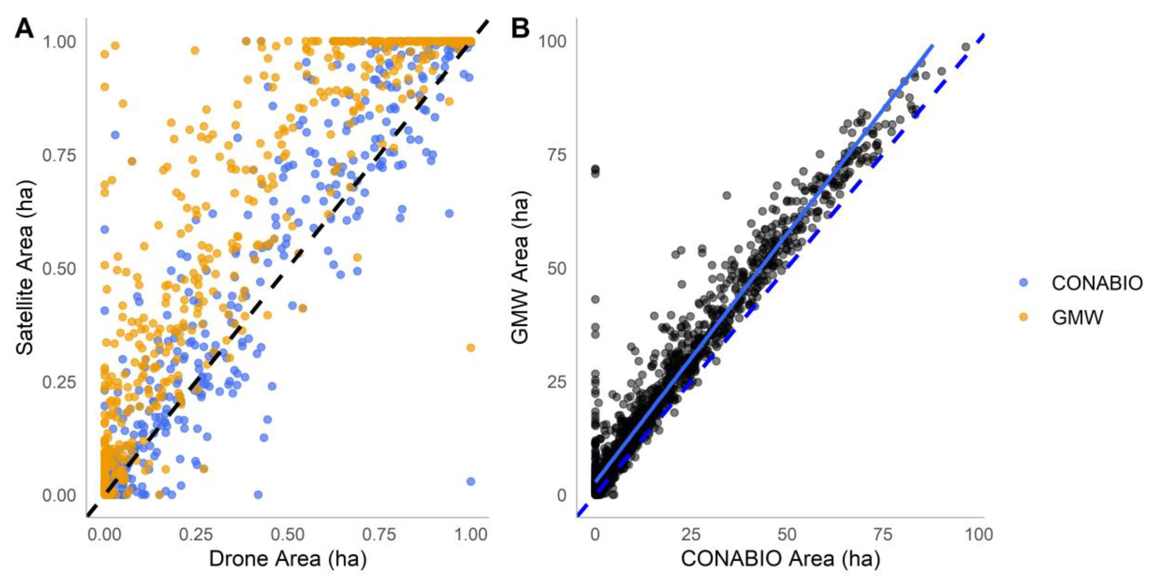
Of 542 fishnet cells sized at one hectare with mangrove registered in CONABIO, GMW, or drone datasets, drones detected a total area of 206.04 ha, while CONABIO detected 232.20 ha and GMW detected 294.33 ha, with drone estimating 11% and 30% less mangrove area, respectively. Drone and CONABIO datasets overlapped in extent by an average of 71% ± 2% (SEM) while drones overlapped with GMW by an average of 78% ± 2% (SEM). On average, drones detected 0.38 ± 0.02 (SEM) ha of mangroves, while CONABIO and GMW detected 0.43 ± 0.016 ha and 0.54 ± 0.017 ha, respectively. Agreement with either satellite sources or drones in regard to mangrove extent is highly variable at lower areas of mangroves (Figure 4B).

We found that consensus on mangrove identification rose with the increase in mangrove area. Regarding an analysis of the average and standard error across datasets, we found that, at an 85% confidence interval, all three datasets were statistically different. However, at a 95% confidence interval, only GMW data were statistically different from both drone and CONABIO datasets. Thus, GMW estimates were significantly higher than both drone and CONABIO estimates, while CONABIO’s was only significantly higher than drone data at 85% confidence.

Through our raster analysis between downsampled drone and GMW mangrove extent, we found an intersection over union for all pixels of 0.68, suggesting a similarity between GMW and at 68% similar. Likewise, the ratio of all drone to all GMW pixels was found to be 0.72. This raster comparison indicated that GMW systemically overestimated mangrove extent compared to downsampled mangrove extent by drones by approximately 30%.

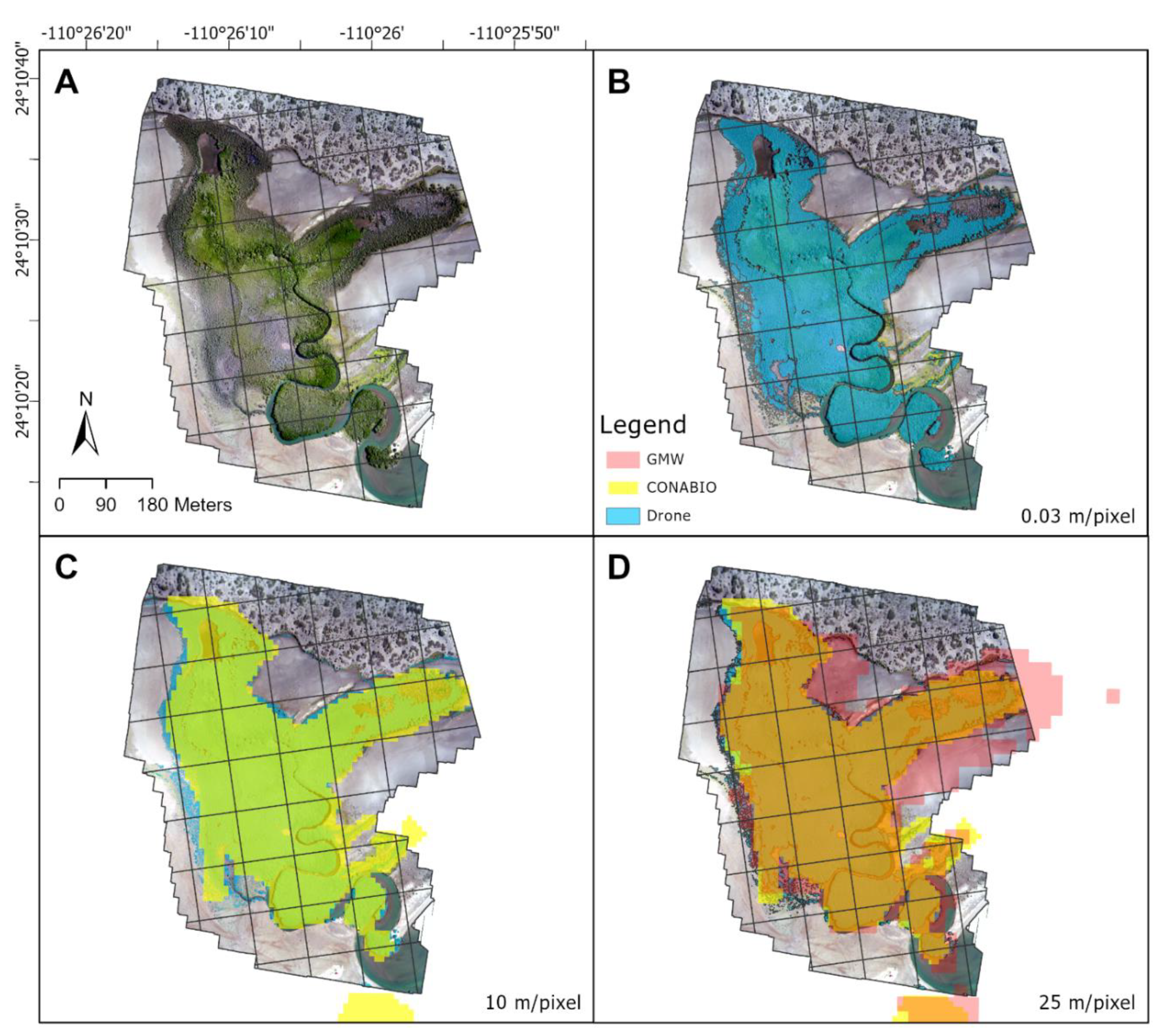
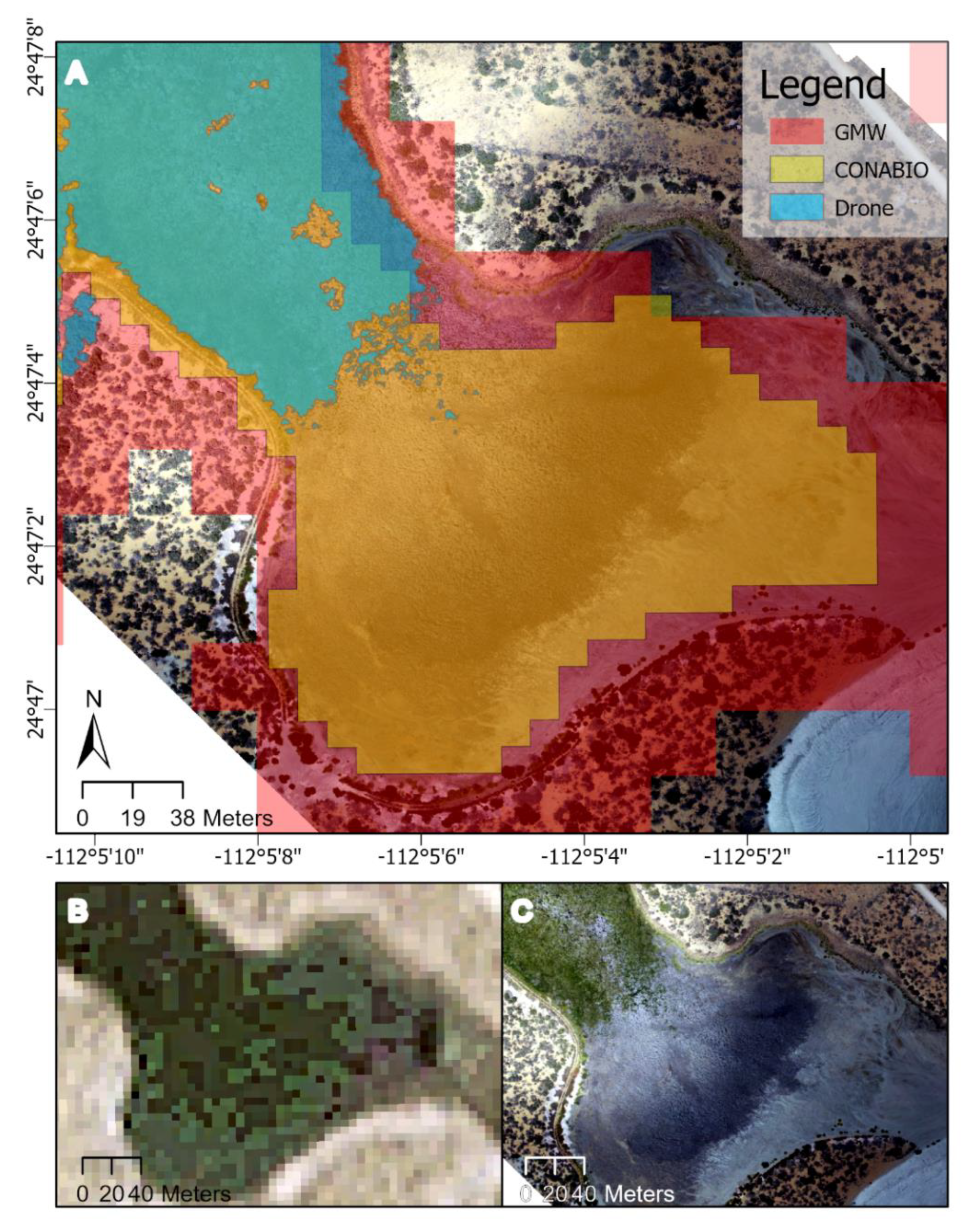
Among all sites, CONABIO and GMW datasets consistently identified bodies of water as mangroves (Figure 5). Lagoons of various sizes were mistakenly labeled as mangroves, as were dirt patches, rivers, and roads. It was common that patches of non-mangrove area, when surrounded by mangroves, were misidentified as mangroves or largely underestimated in area.

3.2. Comparing Satellite-Based Datasets for BCS

Of 1678 fishnet cells sized at 100 hectares with mangrove area registered in either GMW or CONABIO dataset for Baja California Sur, CONABIO’s data resulted in a total area of 26,843.44 ha, while GMW registered 34,052.54 ha. The area of mangrove identified in either CONABIO or GMW datasets totaled 35,200.97 ha, while the area of intersection or overlap totaled 25,695.23 ha (73%). The difference in area averaged 5.66 ± 0.15 (SEM) ha per cell, with a range of 0.00 to 71.82 ha. On average, the two datasets’ mangrove coverage overlapped 50.68% ± 0.78% (SEM). The percent intersection ranged from 0.00% to 98.36%.

GMW data significantly overestimated mangrove area compared to that of CONABIO (Figure 4B, p < 2.2 × 10⁻¹⁶. Of the area identified by CONABIO as mangrove, on average, 6.83% ± 0.38% (SEM) disagreed with the area identified by GMW. Conversely, on average, 42.48% ± 0.80% (SEM) of GMW data disagreed with CONABIO data.

3.3. Convolution Analysis of GMW and Drone Datasets

From our convolution analysis, we calculated averages of drone-identified mangrove extent (Figure 6) and correction factors (

Table 1. Table of averages for mangrove extent based on convolution analyses of GMW data.

Gridcode	Correction Factor	Count
0	0.0%	1558
1	4.14%	376
2	5.79%	324
3	10.02%	399
4	13.10%	244
5	13.30%	71
6	12.60%	26
7	14.98%	8
8	30.22%	1
100	1.36%	2
101	0.88%	6
102	32.15%	14
103	17.80%	91
104	24.21%	231
105	37.97%	427
106	42.02%	351
107	54.06%	452
108	82.75%	3461

) for each gridcode. With the exception of the gridcode 0, gridcode averages were the same as the correction factors. Gridcode 0 is corrected to model zero mangrove coverage because this gridcode is inclusive of habitats that do not have any mangroves (e.g., open ocean, inland, etc.). As such, to ensure accuracy for these large swaths of non-mangrove area, gridcode 0 was assigned a correction factor of 0%.

Gridcodes 1–8 and 100–104 represented patchy mangrove forests, while gridcodes 105–108 represented more uniform mangrove forests. Counts of gridcode 0 and 108 were, respectively, three times and seven times higher than that of the next highest gridcode (107), indicating a clustering of non-mangrove cells and enclosed mangrove cells from GMW. This is further highlighted by the rarity of gridcodes 7, 8, 100, and 101 (Figure 6A). Our results further demonstrated that, as GMW increased gridcode values (as the last digit in the gridcode approaches 8), there were increased drone estimations of mangrove coverage. As gridcode approached 0 and 108, there was increased agreement between satellites and drone estimations of non-mangrove and mangrove habitat, respectively (Figure 6A).

Finally, for all BCS, we found an area of 24,901.66 ha of mangroves after correction. This area is 8% less than CONABIO’s area of 26,843.44 ha and 17% less than GMW’s area of 34,052.54 ha.

3.4. Dramatic Mangrove Loss Event

In one case, we found that CONABIO (data from 2015) and GMW (data from 2016) surveyed mangroves that were no longer present by the time this study began in 2018. To determine this, we downloaded RapidEye 5 m imagery from February 2015, similar to what CONABIO may have had access to, and performed a comparison for Puerto San Carlos, BCS (Figure 7) [26]. In this instance, the difference in mangrove extent was not due to error on mangrove identification, but rather widespread die-off of mangroves due to anthropogenic activity. Dredged sediment had been placed at the end of this mangrove forest, thereby impacting the forest during this three-year period. Drones estimated an extent of 4.3 ha, while CONABIO estimated 6.6 ha and GMW estimated 11.5 ha, resulting in a discrepancy of 2.3–7.2 ha contributed by the dredging event.

4. Discussion

As decision-making around mangrove conservation relies heavily on mangrove extent, there is a need to increase the accuracy of current local and global mangrove extent data. To address this, we conducted analyses of extent maps from GMW, CONABIO, and drones, to disentangle the differences in classified mangrove area and to identify opportunities for improving satellite datasets at the local scale. This study outlines a method to produce local correction factors to GMW mangrove extent based on drone imagery.

4.1. Comparing Mangrove Extent from CONABIO, GMW, and Drone Datasets

On average, GMW estimated greater mangrove extent compared to CONABIO and drone measurements, which corresponds with their use of coarser imagery. Likewise, CONABIO and GMW datasets demonstrated higher variability of mangrove measurements in cells with lower mangrove extent, and higher agreement in areas with greater extent (Figure 4). We downsampled our drone extent produced from shapefiles, and by comparing them to the GMW mangrove extent, we concluded that, even at the same resolution, GMW systematically overestimates mangrove extent. This overestimation is further exemplified in our convolution analysis with GMW, in which clustered GMW pixels—representing greater mangrove extent—corresponded with higher averages of mangrove extent measured by drones (Figure 6A). Areas that were consistently overestimated by satellite-based extent maps are where rivers and lagoons are present and patches of enclosed non-mangrove habitat (Figure 5). With drones providing an avenue for precise photo interpretation, we can leverage the tool to produce high-resolution imagery and generate correction factors.

Though both CONABIO and GMW datasets quoted an accuracy of above 90%, our results show that, in the local region of Baja California Sur, accuracy dips to 85% and 77%, respectively. Our results are in line with Bunting et al.’s notes that GMW has the greatest errors with fine-scale features, common to our drone dataset (2018).

4.2. Correction Factors

When leveraging remote-sensing applications, one must consider that regional differences in mangrove communities and environments will require regional-scale evaluation and training [11]. Drones fulfill the niche of very high-resolution imagery needed for regional validation, and they can be used to bridge the gap between the most advanced satellites and “in-person” observations.

In regions such as Baja California Sur, mangroves tend to form elongated patches along coasts: this elongated and highly fragmented structure will result in higher numbers of lower-valued GMW gridcodes (last digit of gridcode approaches 0). Our results demonstrate that these regions are especially susceptible to overestimation by GMW (as much as 99% correction on a raster cell) and can greatly benefit from corrections described in this study. It is worthwhile to note that, based on our results, gridcodes 1–8 tend to represent areas where GMW underestimated mangrove area, as GMW classified these cells as “non-mangrove” despite there being partial mangrove coverage (Figure 6B). Conversely, gridocodes 100–108 tend to represent areas where GMW overestimated mangrove area, as GMW classified these cells as “mangrove”, despite partial non-mangrove coverage.

Based on our framework validation presented in Section 2.4.3, we determined that drones can be used to generate a set of correction factors that can accurately adjust GMW extent, and applied our set of correction factors from our sites to all of the mangroves in BCS. The corrected BCS extent is 8% less than CONABIO’s estimate and 17% less than GMW’s estimate. This pattern agrees with our results from Section 3.1, in that extent estimations from drones are lower than CONABIO (by 11%) and GMW (30%). The discrepancy of GMW and drone generated/corrected extent between the site level (30%) and a state level (17%) was due to the larger forests that were analyzed at the state level, such as mangroves found in Magdalena Bay [15]. Our results demonstrate that, as gridcodes approach the value of 108 (representative of fuller mangrove forests), GMW and drone estimations agree. Across BCS, the cell count with a gridcode value of 108 is 8 times more plentiful than the gridcode with the next highest count. Thus, this dominance of high gridcode cell values across all of BCS reduces GMW’s overestimation of mangrove area, but it further highlights the value of these correction factors for local and fragmented areas.

Using Correction Factors and the Framework

The creation and use of the correction factors for site-specific and state-wide adjustments of mangrove extent exemplifies how this framework for correcting satellite-based estimations of mangroves can be extended to areas without drone imagery. Thus, this framework is applicable to both stakeholders with and without access to drones.

If an interested party does not have access to drones, they should first conduct a convolution analysis of the GMW extent for their area of interest. They may then use the correction factors presented in this study if their study sites include mangrove forests with similar bioclimatic conditions to BCS (Table 1). Using the results of the convolution analysis for their area of interest and tallying up the cell count for each gridcode, they can apply our correction factors (Equation (1)) per gridcode and sum the resulting mangrove areas across the gridcodes, thereby adjusting GMW estimates for their local mangroves.

If an interested party does have access to drones, they have the opportunity to implement the framework to develop regional correction factors anywhere with mangroves. In this case, we also recommend that they begin by conducting a convolution analysis. Because of the low agreement between satellites and drones in gridcodes 6–8 and 100 to 104, drones are particularly advantageous in these cells. Stakeholders can use the convolution analysis to ensure that all gridcodes are imaged by drones to develop correction factors for their own gridcode analysis. This will require, as our framework shows (Figure 2), distinguishing and labeling mangrove and nonmangrove habitat within the drone imagery. Thus, these new regional correction factors can be used with mangroves in similar environments.

As such, our convolution framework expands the application of drone imagery to be much larger than its photographic footprint. Our framework demonstrates how drones ultimately complement satellite imagery of mangroves and can be leveraged to produce higher accuracy local mangrove extent maps.

4.3. Limitations

Drones have many advantages, such as capturing imagery at high resolutions and greater flexibility on where and when to fly, but their coverage is far more limited than that of satellites. Additional logistical shortcomings of using drones include restrictions by local regulations, expertise, and limited financial resources for procurement of equipment/software [34].

One limitation of this study is the opportunistic sampling of drone imagery. While the samples are limited to mangrove forests in La Paz and Puerto San Carlos rather than the ideal random sampling throughout the entire BCS state, these sites are assumed to be representatives of mangroves in the Gulf of California and Pacific coast of the Baja California Peninsula, respectively. We thereby recommend that correction factors be produced and tested in mangrove forests in regions with higher rainfall. High-resolution imagery of drones and subsequent correction factors may be more advantageous here, where mangrove forests intermingle with other jungle vegetation and increase the difficulty of distinction at coarse resolution. Our study also demonstrated high agreement between satellites and drone at around 0% and 100% mangrove coverage. This clustering can be attributed to the limit of one-hectare analysis, which thereby constrains the upper threshold of variability, and the large resolution size of GMW imagery. Differences in labeling method may also contribute to the difference in reported accuracy.

Lastly, while we used the most recent years available for our data—2016 for GMW, 2015 for CONABIO, and 2018/2019 for drones—changes in mangrove extent and water levels could have occurred among the timings of collection. This is evidenced by the significant loss of mangroves attributing to differences in mangrove extent among datasets (Figure 7). We found that our correction factors as described in Section 3.3 may be limited in their application in regard to the difference in time of when drone and satellite imagery were captured and if dramatic mangrove loss occurs. Withholding extreme cases of mangrove loss, for this study, the state of BCS generally has an annual deforestation rate of 0.225% [35], which would amount to a total of 0.675% difference in mangrove extent and is considered insignificant beyond the example described. Variation in water level (i.e., tidal levels) may explain some of the discrepancies between satellite and drones, assigning larger error to satellite data. However, the consistency of the overestimation we are measuring cannot be exclusively from these events. Therefore, despite these limitations, we believe our method stands robust and can still achieve an improvement of area estimations.

4.4. Potential of Machine Learning

The rise of machine-learning applications provides an opportunity for mangrove conservation to use drone imagery and labels to fine-tune estimations produced by satellites. Hand-labeling of mangroves took over 1000 h for just over 455 hectares imaged by drones, but these labeled data can be leveraged as training data for machine learning algorithms. Global Mangrove Watch has already demonstrated the use of machine learning algorithms to measure global mangrove extent almost annually [14]. There is potential for different resolution imagery to be integrated to produce algorithms for mangrove detection that are more scalable than just drone-based monitoring, but with higher accuracy than current satellite-based estimations, especially with the availability of higher resolution satellite imagery from Digital Globe and Planet Labs [36]. This integration can lead to the development of fine-spatial resolution mapping on a global level [7].

4.5. Management Implications

National decisions regarding climate sustainability loom ahead. The Convention of Biodiversity is set to convene to adopt a post-2020 framework, and Nationally Determined Contributions of the Paris Agreement for the next five years are to be submitted marked with increasing ambition. Additionally, 2021–2030 is the United Nations Decade of Ocean Science for Sustainable Development. Mangroves are poised to serve as solutions for climate adaption and mitigation, but they lack the support needed for effective implementation [5,35,37]. As an essential ocean variable that provides high social value, mangroves require higher spatial and temporal monitoring, especially in areas that are at high risk of loss [4]. Desert mangroves in regions such as our study area, Baja California Sur, have been shown to store large amounts of carbon, up to 3000 Mg C/ha, and, thus, accurately monitoring these systems is of importance for climate mitigation [38].

The overestimation of mangrove coverage due to satellite-based methods may provide a false sense of security or overconfidence in the area of mangroves that the world has, and their capacity to mitigate climate change. Specifically, overestimation of mangrove extent results in the miscalculation of total global economic value of mangrove ecosystem services and the overestimation of the capacity for mangroves to mitigate climate change. This is due to the fact that both ecosystem service value and climate mitigation capacity are calculated based on mangrove extent [39,40]. Likewise, as our case studies in Puerto San Carlos and La Paz demonstrate, as loss of mangroves occurs, it is important to intervene and take timely action rather than a passive, backward-looking approach. Fine-scale monitoring in both resolution and time can provide details on deforestation activities as they begin, not after large areas have already been deforested. This is especially crucial for local enforcement and governance in light of climate change, as mangrove deforestation releases carbon stores and further contributes to climate warming [34,41].

As we increasingly lean on technology to produce more accurate and timely baselines, we must synchronize the use of satellites and drones, to monitor at the same resolution and pace as our changing environment. Ultimately, satellites and drones are tools that can facilitate collaborations among various stakeholders with different but complementary interests. Both tools can be integrated into communities to empower local people and increase local capacity to better manage natural resources in a cost-efficient manner [42]. In complementing drones with satellites in the hands of the local community, mangrove monitoring can transition from the passive documentation of changes in extent to active management and intervention.

5. Conclusions

From ecosystem valuation to international commitments, the use, management, and conservation of mangroves relies on mangrove extent maps. In particular, mangrove extent is referenced as a metric to achieve international conservation commitments (i.e., Ramsar Convention, Sustainable Development Goals), and researchers have turned to remote sensing tools, to better track this shifting baseline. This study compares satellite mangrove extent from the CONABIO (2015) and the GMW (2016) with in situ drone imagery in Baja California Sur, Mexico (2018, 2019). We found that satellite-based mangrove extent maps tend to overestimate mangrove coverage, especially at the local scale. We developed a framework and correction factors by using drone imagery and convolution analysis to correct these maps. This framework provides a method to correct GMW extent data and reveals a key avenue for using drones to enhance satellite imagery.

Drones complement satellite imagery and will enable researchers, resource managers, and other end-users to improve current and future datasets on mangrove extent, by highlighting systematic errors and reducing overestimation. By providing a more accurate map of mangrove extent, the valuation of mangrove ecosystem services, including estimations of mangroves’ capacity to mitigate climate change, will more accurately capture reality. Together, drones and satellites can better inform mangrove management and support the achievement of international conservation commitments.