An Improved Correction Method of Nighttime Light Data Based on EVI and WorldPop Data

Abstract

Defense Meteorological Satellite Program’s Operational Linescan System (DMSP/OLS) data has the shortcomings of discontinuous and pixel saturation effect. It was also incompatible with the Soumi National Polar-Orbiting Partnership Visible Infrared Imaging Radiometer Suite (NPP/VIIRS) data. In view those shortcomings, this research put forward the WorldPop and the enhanced vegetation index (EVI) adjusted nighttime light (WEANTL) using EVI and WorldPop data to achieve intercalibration and saturation correction of DMSP/OLS data. A long time series of nighttime light images of china from 2001 to 2018 was constructed by fitting the DMSP/OLS data and NPP/VIIRS data. Corrected nighttime light images were examined to discuss the estimation ability of gross domestic product (GDP) and electric power consumption (EPC) on national and provincial scales, respectively. The results indicated that, (1) after correction, the nighttime light (NTL) data can guarantee the growth trend on national and regional scales, and the interannual volatility of the corrected NTL data is lower than that of the uncorrected NTL data; (2) on the national scale, compared with the established model of NTL data and GDP data (NTL-GDP), the determination coefficient (R²) and the mean absolute relative error (MARE) are 0.981 and 8.518%. The R² and MARE of the established model of NTL data and EPC data (NTL-EPC) were 0.990 and 4.655%; (3) on the provincial scale, the R² and MARE of NTL-GDP model under the provincial units are 0.7386 and 38.599%. The R² value and MARE of NTL-EPC model are 0.8927 and 29.319%; (4) on the provincial scale, the R² and MARE of NTL-GDP model on time series are 0.9667 and 10.877%. The R² and MARE of NTL-GDP model on time series are 0.9720 and 6.435%; the established TNL-GDP and TNL-EPC models with 30 provinces data all passed the F-test at the 0.001 level; (5) the prediction accuracy of GDP and EPC on time series was nearly 100%. Therefore, the correction method provided in this research can be applied in estimating the GDP and EPC on multiple scales reliably and accurately.

1. Introduction

Night light remote sensing, as an active branch of remote sensing [1], can obtain the information of visible light and near infrared electromagnetic wave emitted from the ground surface on cloudless nights [2] It can reflect the urban night lighting and capture the night lighting of fishing boats [3], natural gas combustion [4], and forest fire light [5]. It intuitively reflects the human activities and social development rules [6] and is widely applied in the estimation of socioeconomic parameters such as GDP [7], population density [8], electric power consumption (EPC) [9], greenhouse gas emissions [10] and poverty index [11]; urban expansion [12] and urbanization research [13]; major events assessment such as energy crisis [14], earthquake [15] and war [16]; environmental effect analysis of urban expansion [17]; light pollution [18] and effect analysis [19]. Consequently, it has become the main data source for monitoring human socioeconomic activities and natural phenomena.

The Defense Meteorological Satellite Program’s Operational Linescan System (DMSP/OLS) and Soumi National Polar-Orbiting Partnership Visible Infrared Imaging Radiometer Suite (NPP/VIIRS) are the most widely used to obtain the nighttime light data. In this research, it provides nighttime light (NTL) data from 1992 to 2013 and 2012 to 2018, which are named as DMSP/OLS and NPP/VIIRS, respectively.

The Operational Linescan System is one of the principal sensors on the DMSP satellite platform. The radiation value detected by OLS sensors at night is four orders of magnitude lower than that of other sensors [20]. Due to the superior performance of OLS sensors, the NTL data is often used for exploring human activities. However, DMSP/OLS data also has a series of shortcomings [21]. Light saturation in the city center, blooming effect, and lack of airborne calibration are the major obstacles to the application of DMSP/OLS data. The light saturation phenomenon is caused by the low 6-bit radiation resolution of OLS sensor. The pixel value of DMSP/OLS data ranges from 0 to 63. When the radiation brightness of a light source in the city center exceeds to the detection upper limit (10⁻⁸ W/ (cm²*sr*um)), the DN values of DMSP/OLS data are all forced to be 63 [22]. Therefore, it is impossible to distinguish the spatial difference of actual lighting intensity in the urban central area where the lighting intensity exceeds the detection limit [23]. Furthermore, the correlation between the detected NTL and economic activity is reduced, which increases errors in the established model [24,25], and limits the application of NTL data [26]. At the same time, DMSP/OLS dataset is made up of NTL data collected by different satellite sensors in different years. In the absence of airborne calibration [4], the night stable light data was affected by the difference of sensors, the difference of satellite cross time, and the influence of the sensor performance degradation [27]. Therefore, the data cannot be directly compared [28]. In addition, the illumination area is overestimated due to the reflection of urban light to urban edge and internal water body, and then increases the error of distribution estimation [29].

In order to improve the accuracy of nighttime light data in representing social and economic activities, many studies have attempted to solve the problems in DMSP/OLS data. Aiming at the saturation problem of DMSP/OLS data, scholars have proposed a series of methods to correct the saturation. The correction method is mainly divided into only using the NTL data and using other satellite data to correct the NTL data. There are three calibration methods that only use the NTL data: (1) radiation calibration desaturation method. This method is used to adjust the sensor gain to make it lower than the typical work settings and obtain the nighttime light change in the city center [30]. The limited nighttime light data obtained can be combined with the nighttime light data obtained under the high gain setting to generate the unsaturated nighttime light data [23]. Although this method can effectively reduce the saturation effect of NTL data, it is labor intensive and cost intensive. Therefore, calibration data only can be obtained with a limited number of years (1996, 1999, 2000, 2002, 2004, 2006, and 2010). (2) Desaturation method based on frequency distribution of the DN value of light pixels [31]. This method is based on the assumption that the variation trend of the DN value of night light in saturated regions which is consistent with that in unsaturated regions, the number of pixels in saturated regions can be predicted by establishing a linear correction model of the number of pixels in unsaturated regions and the DN value [32]. Letu et al. used the cubic regression model to construct the DN value frequency of light pixels to correct the saturation problem of light images on the basis of the linear correction model [33]. This method is a desaturation method on the regional scale which is not suitable for the pixel scale. (3) The desaturation method based on the invariant target area. This method realizes the saturation correction of the NTL image by determining the corresponding relationship between DN value in the invariant target area of the stable image and Radiance Calibrated Nighttime Lights (RCNTL). Letu et al. realized the correction of the light data of the saturated region in the year of 1999 by constructing a regression model of the nighttime light data of the unsaturated region of the target region in 1999 and the nighttime light data of the radiometric calibration image in 1996–1997 [24]. Wu et al. used the NTL data of RCNTL in 2006 to achieve the correction of DMSP/OLS saturated images by defining Mauritius, Puerto Rico, and Okinawa as invariant target areas [34]. This correction method can reduce the saturation of the pixel to a certain extent, but the saturated pixel is corrected to the same DN value through the regression model, which means that the corrected pixels lack spatial difference and cannot reflect the real nighttime light data. At the same time, saturation correction will lead to distortion of unsaturated pixels in suburban and rural areas of underdeveloped areas [35]. There are also three calibration methods that use other satellite data to correct the NTL data: (1) correction of nighttime light data based on vegetation index. Vegetation adjusted normalized urban index (VANUI) [36,37] was proposed by combining normalized difference vegetation index (NDVI) with DMSP/OLS data based on the principle that urban characteristics (including nighttime light) should be inversely proportional to vegetation coverage [38]. Enhanced vegetation index adjusted nighttime light index (EANTLI) [39,40] was proposed combined with the advantages of enhanced vegetation index (EVI) [41] to make it impossible for VANUI to effectively highlight the difference of nighttime light intensity in saturated areas under the rapid urbanization process in China and other countries. EVI data is the vegetation index obtained by the calculation of infrared band, near-infrared band, and blue light band [42] in remote sensing data. It is an important numerical expression method for monitoring the growth information of surface vegetation, which can effectively describe the growth and biomass information of green plants. However, at present, this method is mostly used to correct DMSP/OLS images of specific years, and rarely to correct long time series DMSP/OLS datasets. Moreover, rare studies have been conducted on the consistency correction of DMSP/OLS data based on EVI correction and NPP/VIIRS data. (2) NTL data was corrected based on surface temperature and vegetation index spatial distribution difference of vegetation was a natural factor and the influence of human factors on the evolution of urban internal structure. LST and EVI Regulated NTL City Index (LERNCI) based on EVI, land surface temperature (LST), and nighttime light data was proposed [43]. LERNCI based on the double correction of LST and EVI can better improve the spatial difference caused by single index correction. (3) Other data to correct the NTL data: GDP data can effectively reflect the urban development vitality. Therefore, a linear model between the GDP grid data of corresponding time and the NTL data of unsaturated areas is constructed, and the NTL data of saturated areas can be calculated by the model to eliminate the saturation phenomenon [44].

In view of the lack of airborne calibration, the invariant region method was used to realize intercalibration of DMSP/OLS data [45]. Assuming that there are relatively unchangeable pixels in the multi time nighttime light image, and building calibration model of invariant pixels in different images, the calibration model is used to correct the corresponding night light image to get comparable night light images. Elvidge et al. [4] assumed that the NTL data of Sicily in Italy remained basically unchanged from 1994 to 2008. Based on the baseline image in F121999, the regression model of other images from 1994 to 2008 was constructed to achieve intercalibration. Liu et al. [46] used the second order regression model to realize intercalibration of Chinese DMSP/OLS data from 1992 to 2008 by taking Jixi city of Heilongjiang province as the invariant target area. The above two intercalibration methods solve the problem of incomparability of DMSP/OLS data, but do not effectively correct the saturation problem in the image. How to effectively solve the problem of data saturation in DMSP/OLS data while solving the problem of data incomparability in DMSP/OLS data is still a hot research topic.

With the attenuation and failure of DMSP/OLS, NPP/VIIRS data became the new generation of NTL data [47]. As NPP/VIIRS data with higher spatial and radiating quality than DMSP/OLS data [48], it addresses the shortcomings existing in DMSP/OLS data (saturation of city center light data and lack of airborne calibration), but the published NPP/VIIRS monthly composites is a preliminary product which has not been filtered to screen out lights from aurora, fires, boats, and other temporal lights. To solve this problem, Li et al. [26] proposed to extract the corresponding pixel in NPP/VIIRS data as the stable pixel in NPP/VIIRS data by using the bright pixel in DMSP/OLS data of 2010. Wu et al. [49] used the bright pixel of an annual composite of 2015 to extract the corresponding pixel in the NPP/VIIRS data from 2015 to 2017 as the stable pixel in the NPP/VIIRS data of respective years. Although the above methods can remove some unstable pixels in the NPP/VIIRS data, the first method to extract the NPP/VIIRS data from 2012 to 2018 will cause more information to be lost in later years due to the rapid urbanization process in China. The second method can better retain the information in NPP/VIIRS data, but some information will be lost from 2016 to 2018.

Moreover, combination of DMSP/OLS data and NPP/VIIRS data to study continuity over long time series has great advantages and prospects in the significant application of NTL data in socioeconomic activity studies. However, the inconsistency between NPP/VIIRS data and DMSP/OLS data is more serious than that between the different products of the DMSP/OLS data [50]. Xu et al. [51] achieved the evaluation of urban land expansion in China from 1992 to 2015 by comparing DMSP/OLS data from 1992 to 2013 and NPP/VIIRS data in 2015, but failed to achieve the fitting of the two data. Li et al. [50] fitted NPP/VIIRS monthly composite product and DMSP/OLS monthly composite product by power function and gaussian low-pass filter, but the data set used was not accessible to the public. Researchers [22,52] constructed the regression model between stable image and RCNTL to realize the correction of DMSP/OLS data, and realized the fitting between the two data by establishing the regression relationship between the total nighttime light of DMSP/OLS data and NPP/VIIRS data on the county scale in 2012 and 2013. However, there are still defects in the process of correcting DMSP/OLS data and NPP/VIIRS data, which reduces the correlation between NTL data and socioeconomic indicators.

Scholars have done a lot of research on the processing of DMSP/OLS data and NPP/VIIRS data, but there are still some limitations in the existing research results: (1) in the saturation correction of DMSP/OLS data, the existing research did not distinguish the spatial differences of the saturated pixels and carried out the saturation correction of the unsaturated pixels, thus failed to effectively correct the saturation of the DMSP/OLS data. (2) When processing the NPP/VIIRS annual image data, the existing research usually mistakenly classified some stable pixels as unstable pixels and lost some effective information. (3) When fitting DMSP/OLS data and NPP/VIIRS data, some scholars used the same fitting function to fit the data of 31 provinces, without considering the data differences of each province, thus reducing the ability of night light data to represent economic data.

Aiming at the problems in the current research, this paper proposes a correction method of nighttime light data using EVI and WorldPop data based on the principle that urban characteristics (including nighttime light) should be inversely proportional to vegetation coverage [38] and directly proportional to population distribution data [53,54], so as to obtain the nighttime light dataset from 2001 to 2018 to represent economic data reliably and accurately. On the basis of related research, the invariant region method is used to realize the intercalibration of the DMSP/OLS data from 2001 to 2013. The annual EVI and WorldPop data from 2001 to 2013 is used to realize the saturation correction of DMSP/OLS data. The corrected unsaturated DMSP/OLS data from 2001 to 2013 is obtained. The corrected DMSP/OLS data and NPP/VIIRS data are fitted by using a regression model to obtain the regional scale DMSP/OLS data from 2001 to 2018. The validity of the correction method is evaluated by constructing indexes such as total nighttime light (TNL), normalized difference index (NDI), and the sum of normalized difference index (SNDI). The correlation between NTL data and GDP or EPC and the relative error of the estimation model are calculated.

2. Study Area and Data

A total of 30 provinces were chosen as the study areas in mainland of China due to the lack of economic statistics from Hong Kong, Macau, Taiwan, and Tibet. For regional comparison, the study area was divided into four regions (Northeast, East, Central and West). These regions, in addition to their geographical location, are a broad reflection of overall differences in socioeconomic development.

Eight types of data were used in this study, including DMSP/OLS data, NPP/VIIRS data, EVI data, WorldPop data, gas combustion area mask, county level administrative boundary vector map, river and lake data, and socioeconomic statistics.

DMSP/OLS night lighting data set from 2001 to 2013 was collected from the website (https://eogdata.mines.edu/dmsp/downloadV4composites.html) of Paynes Institute for Public Policy, Colorado School of Mines. There are three annual average data types in the dataset which are cloud-free coverage, average visible light, and stable light. Among the three types of data, the stable light data contains light from cities, towns, and other locations with continuous lighting, while fires, volcanoes, background noise, and other transient events are discarded [27]. The 20 images were captured by four different DMSP satellites, F14 (2001–2003), F15 (2001–2007), F16 (2004–2009), and F18 (2010–2013). In this paper, the radiometric calibration product of F162010 (https://eogdata.mines.edu/dmsp/download_radcal.html) was used to compare the influence of calibration method on the saturation effect of nighttime lighting data.

NPP/VIIRS data from 2012 to 2018 was also collected from the website of Paynes Institute for Public Policy, Colorado School of Mines (https://eogdata.mines.edu/download_dnb_composites.html). The images used for this study were monthly VIIRS DNB composite from 2012 to 2018 and two annual composites of 2015 and 2016. However, the NPP/VIIRS monthly composite was not filtered to eliminate light detection associated with gas flares, fires, volcanoes or auroras, and the data set was not processed to eliminate background noise. Temporary lighting and background noise were eliminated in the annual composite image.

EVI data is the EVI monthly composite of the moderate resolution imaging spectroradiometer (MODIS). The data set was provided by Geospatial Data Cloud site, Computer Network Information Center, Chinese Academy of Sciences. (http://www.gscloud.cn).

The WorldPop dataset was developed by the WorldPop Project (https://www.worldpop.org). The dataset provides annual gridded population data from the 2000–2020 period, with a spatial resolution of 100 m. The input variables of WorldPop include the most recent official census population data and a wide range of spatial ancillary datasets. The spatial datasets include settlement locations and extents, nighttime satellite images, land cover, roads, building maps, health facility locations, vegetation, topography, and refugee camps. A random forest regression tree-based mapping approach was used to generate a predictive weighting layer to reallocate population counts into gridded pixels [55]. The WorldPop dataset has two products, one is the number of people per hectare, the other is the number of people per grid, and the latter dataset was used in this paper.

Gas burning zones are generated due to insufficient infrastructure in the oil producing areas to make full use of natural gas. The data of the gas burning area used in this paper can be downloaded from the website of Paynes Institute for Public Policy, Colorado School of Mines (https://eogdata.mines.edu/download_global_flare.html).

Vector maps of China’s county-level administrative boundaries and rivers and lakes data were obtained from 1:400 million database in the National Fundamental Geographic Information System. All nighttime lighting data were extracted according to China’s administrative boundary.

The socioeconomic statistics from 2002 to 2019 were provided by the China statistical yearbook which was published by China National Bureau of statistics (http://www.stats.gov.cn/tjsj/ndsj/). These include two attributes for reference: gross domestic product (GDP) and electric power consumption (EPC). The unit of the GDP is billion RMB, and the unit of EPC is billion·kilowatt·h⁻¹.

Agriculture is an important part of social and economic activities, especially in a traditional agricultural country like China. However, most of the agricultural production is located in the darker area of the nighttime light image, so the nighttime light data cannot represent the agricultural part of economic activities [56]. Therefore, it is necessary to remove the contribution of agricultural sector to economic activities when using nighttime data to predict GDP. The GDP data in the following paragraphs are all subtracting the data of the agricultural sector.

3. Methodology

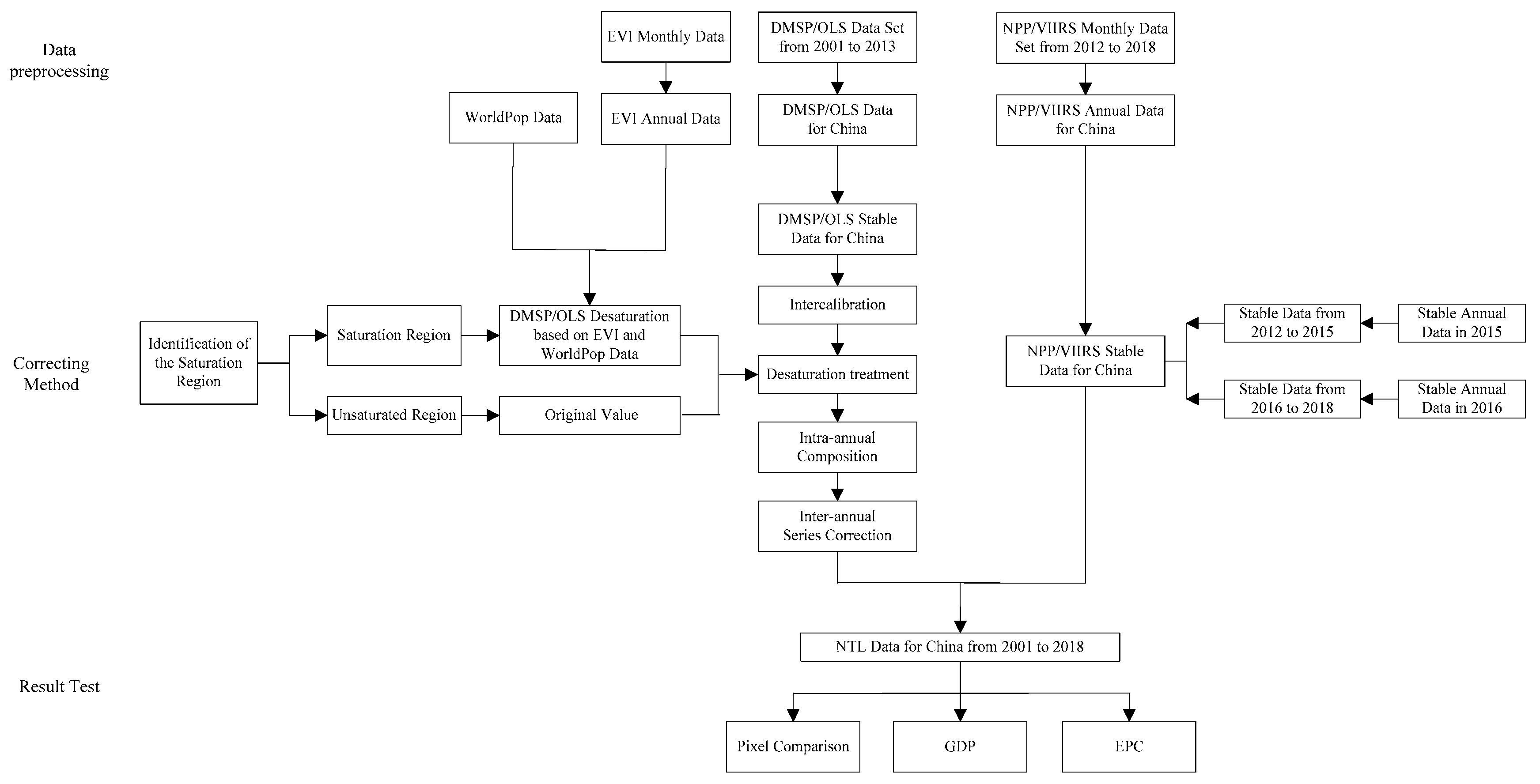
This section introduces the method of NTL data processing and result verification. The method is divided into three steps (Figure 1): (1) data preprocessing: preprocessing of DMSP/OLS data, NPP/VIIRS data, and EVI data. (2) Calibration method: the calibration method is divided into DMSP/OLS data calibration method and NPP/VIIRS data calibration method. The DMSP/OLS data and NPP/VIIRS data of the same year after calibration are fitted and analyzed by linear regression model to obtain a long time series NTL data in China. (3) Result verification: the accuracy of the results was quantitatively verified by comparing the corrected pixels and analyzing the linear relationship between GDP, EPC, and NTL data.

3.1. Data Preprocessing

3.1.1. Image Clipping and Resampling

The coordinate system of DMSP/DLS (version 4) nonradiometric calibrated night light intensity image from 2001 to 2013, NPP/VIIRS composite from April in 2012 to December in 2018, and NPP/VIIRS annual composite of 2015 and 2016 are all WGS-84 (World Geodetic System 1984). With the increase of latitude, image mesh decreases [4]. To avoid the influence of image grid deformation on night image data and facilitate the calculation of light pixel area, all night light intensity images were first extracted in the administrative region of China. Then, the extracted image coordinate system was transformed to Lambert equal area projection coordinate system and the nearest-neighbor resampling algorithm (NEAREST) was used to resample the mesh in the image to 1000 m.

3.1.2. Removal of Water and Gas Burning Areas

The reliability of NTL data can be further improved by removing NTL data from water and natural gas combustion areas in DMSP/OLS and NPP/VIIRS images [57].

3.1.3. Preprocessing of NPP/VIIRS Data

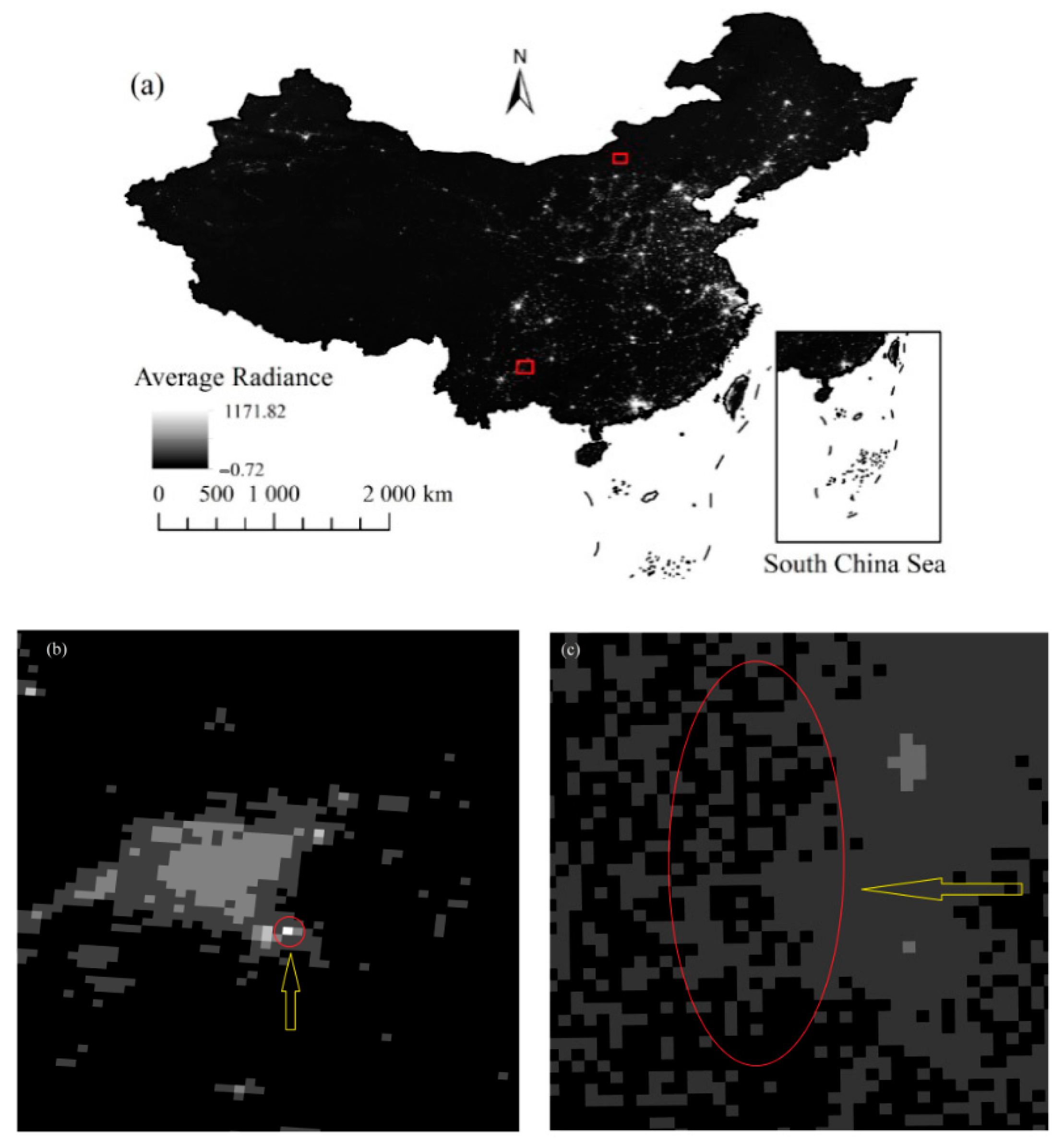
Radiation value of night light image data in January 2013 is from −0.72 to 1171.82 (Figure 2), but the image is a preliminary data set which is not filtered to eliminate light detection associated with auroras, fires, ships, and other temporary lights [22]. Therefore, it is necessary to reduce the impact of unstable night lighting and background noise on nighttime lighting images. Usually, an appropriate threshold interval is set to remove abnormal values (high and low values) to extract effective nighttime lighting images. In general, threshold interval can be set by percentage method, total light area increase method, and economic intensity method. In this paper, the economic intensity method was used to extract the effective night light image [58]. Beijing, Shanghai, and Guangzhou are the three most developed cities in China. Therefore, the pixel values of all regions in China should theoretically be less than the maximum values of these three cities. Hence, the maximum radiation value of these three cities was taken as the upper limit value of the threshold interval. For example, in January 2013, the maximum radiation value of Beijing, Shanghai, and Guangzhou was 255.68, so 255.68 was used as threshold value to correct abnormal value of China nighttime light image data in January 2013. The pixel points higher than the threshold value in the nighttime light image were identified as the abnormal pixel points. As the abnormal pixel points may gather, in order to ensure the complete elimination of the abnormal pixel points, the average value of 24 pixels around the outliers was assigned to the outliers with average filtering method [59]. After processing, the corrected NTL data in January 2013 were all lower than 255.68.

Table A1. Upper limit of nighttime thresholds for each month from 2012 to 2018.

	1	2	3	4	5	6	7	8	9	10	11	12
2012	-	-	-	238.61	-	-	-	349.68	337.06	323.07	490.64	323.48
2013	255.68	220.03	212.53	251.44	-	-	-	382.74	226.43	292.99	407.68	342.24
2014	268.78	249.83	277.99	216.80	-	-	-	249.16	308.24	278.46	335.64	358.81
2015	291.88	259.75	219.36	309.58	-	-	-	296.66	340.50	314.39	308.13	274.78
2016	289.55	288.25	217.33	245.23	-	-	-	916.30	2465.71	270.01	810.06	289.59
2017	242.50	277.57	412.74	260.47	-	-	-	348.81	256.25	429.59	258.93	321.35
2018	391.84	395.66	380.31	309.81	-	-	-	395.62	1101.97	336.33	239.81	746.02

in the Appendix A shows the upper limit of nighttime thresholds for each month from 2012 to 2018.

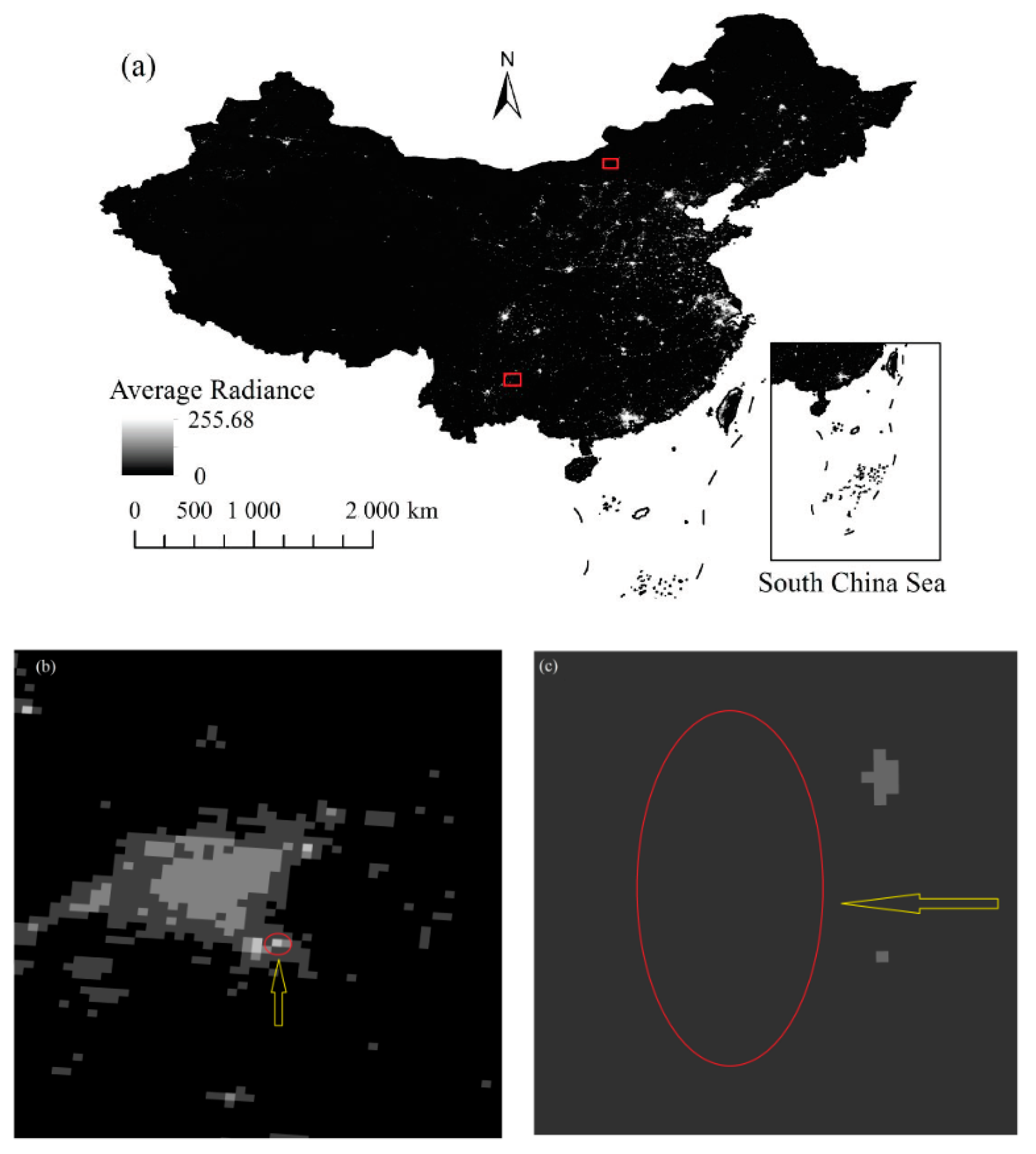
In general, NPP/VIIRS monthly composite image has negative radiation value pixels. This is because in the dark current correction process, the average night ocean data in the northern hemisphere is used and there is system noise which makes the pixels in the dark area appear as negative values [60]. Therefore, the pixels with negative radiation value are assigned as zero [61]. After the above two processing steps, the corrected nighttime light image of China in January 2013 was obtained as shown in Figure 3. Compared with Figure 2 and Figure 3, it can be found that after the above processing, the abnormally highlighted pixels and the pixels with radiation value less than zero were processed.

Therefore, 60 NPP/VIIRS monthly corrected nighttime light images from 2012 to 2018 were obtained by the above correction methods, and then Formula (1) was used to process the NPP/VIIRS monthly corrected nighttime light images to obtain the preliminary corrected NPP/VIIRS annual composite images from 2012 to 2018.

$$D{N}_y=\frac{{\displaystyle {\displaystyle \sum }_{i=1}^{12}}D{N}_i}{n}$$

(1)

where, $D{N}_y$ is the annual average nighttime light value, and $D{N}_i$ is the monthly average nighttime light value in ith month. Due to the serious lack of NPP/VIIRS data from May to July, they are not involved in the calculation, hence: $i\ne$ 5, 6, 7; n = 9.

3.1.4. Preprocessing of EVI Data

In order to reduce the sensitivity of seasonal and grade fluctuations [37], Formula (2) was used in this paper to process monthly products to obtain annual average EVI data instead of annual maximum EVI data. Due to the lack of monthly EVI data in 2004 and 2008, the average EVI data in 2003 and 2005 was assigned to the average EVI data in 2004, and the average EVI data in 2007 and 2009 was assigned to the average EVI data in 2008. The 13 EVI images calculated from 2001 to 2013 were extracted from the administrative region of China by ArcGIS, and then the extracted image coordinate system was transformed to Lambert equal area projection coordinate system and the nearest-neighbor resampling algorithm (NEAREST) was used to resample the mesh in the image to 1000 m.

$$EV{I}_y=\frac{{\displaystyle {\displaystyle \sum }_{i=1}^{12}}EV{I}_i}{n}$$

(2)

where, $EV{I}_y$ is the annual average EVI value, and $EV{I}_i$ is the monthly average EVI value in ith month.

3.2. DMSP/OLS Data Calibration Method

Since DMSP/OLS data was not radiometric calibrated, the existing DMSP/OLS nighttime light image data set was obtained by six different sensors. The image data of different years cannot be directly compared due to the differences in the performance of different sensors, the decline of their detection performance with the use time, and the different imaging environment. Moreover, due to the upper limit of sensor detection, pixel saturation exists in the city center. Based on the principle that urban characteristics (including nighttime light) should be inversely proportional to vegetation coverage [38] and directly proportional to population distribution data [53,54], WorldPop and the enhanced vegetation index adjusted nighttime light (WEANTL) constructed by EVI, WorldPop, and DMSP/OLS data can restore the light intensity in the saturated area to a certain extent, alleviate the saturation phenomenon of light intensity in the urban center, increase the spatial difference of light intensity, and make the nighttime light data better reflect social and economic activities. Therefore, in this paper, the invariant region method was used to conduct intercalibration of DMSP/OLS data, and then EVI and WorldPop data were used to conduct saturation calibration of DMSP/OLS data, so as to obtain higher quality and analyzable long time series nighttime light images.

3.2.1. Intercalibration

Obtaining historical stable images in China, it is necessary to consider the image data collected by the same sensor in different years and different sensors in the same year. The stable bright pixels obtained by different sensors in the same year should be consistent. The bright pixel of the previous year must be the stable bright pixel of the next year [62].

Processing of nighttime light images in China from 2001 to 2013: in ArcGIS software, the DN value of pixels which is larger than zero is assigned as one and the DN of pixels which is equal to zero remains unchanged by using the grid calculator tool. By assuming that all the pixels is which DN values are equal to one in the processed nighttime light image of F182013 are all stable light pixels, after image intersection processing between the nighttime light image of F182013 and nighttime light image of F182012, the pixels in which DN values are equal to one in the nighttime light image is the stable bright pixel of 2012. The processed nighttime light image is called the stable nighttime light image mask. If there are multiple nighttime light images in the same year, such as the nighttime light image of F162007 and F152007, the stable nighttime light image mask of 2008 and the nighttime light image of F162007 and F152007 processed by binary method are intersecting, processed to obtain the stable nighttime light image mask of 2007. By that analogy, the stable nighttime light image masks from 2001 to 2013 are obtained.

Obtaining the stable night light image of China: each stable nighttime light image mask is used to remove the unstable pixels from the nighttime light image of the corresponding year, and get the stable nighttime light image of China after removing the unstable pixels.

Sample data area and reference calibration nighttime light image selected: according to the principle of small interannual fluctuation of DN values and wide dynamic range distribution in the year [46], Jixi city, Heilongjiang province [63] was selected as the sample area. F162007 nighttime light image with high total gray value and good continuity was used as the reference calibration nighttime light image [62].

Correction model determined: the single quadratic regression model shown in Formula (3) is used to fit and regress the image data of Jixi City in each year with the reference nighttime light image (F162007). The regression parameters of each image are shown in

Table A2. Intercalibration model regression parameters of DMSP/OLS image

Satellite	Year	a	b	c	R2	Standard Error
F14	2001	−0.002	1.118	0.274	0.845	1.765
	2002	−0.007	1.28	0.268	0.803	1.990
	2003	−0.009	1.447	0.224	0.860	1.678
F15	2001	−0.001	1.054	0.266	0.808	1.965
	2002	−0.0001	1.004	0.237	0.849	1.745
	2003	−0.012	1.652	0.229	0.830	1.848
	2004	−0.011	1.549	0.155	0.881	1.547
	2005	−0.006	1.393	0.139	0.886	1.514
	2006	−0.006	1.35	0.138	0.941	1.085
	2007	−0.005	1.313	0.016	0.980	0.637
F16	2004	−0.004	1.15	0.152	0.865	1.647
	2005	−0.003	1.249	0.114	0.930	1.185
	2006	−0.003	1.227	0.094	0.952	0.982
	2007	0	1	0	1	0
	2008	0.001	0.913	0.013	0.962	0.877
	2009	0.003	0.671	0.011	0.922	1.255
F17	2010	0.005	0.486	0	0.881	1.550
	2011	0.001	0.732	0.005	0.866	1.643
	2012	0.003	0.586	0.004	0.893	1.470
	2013	0.005	0.394	−0.103	0.856	1.704

in the Appendix A. The regression model of the corresponding year is used to regress and correct the obtained DN value of regional stable nighttime light images in China.

$$D{N}_{correct}=a\times D{N}^2+b\times DN+c$$

(3)

where, $D{N}_{correct}$ is the DN value after intercalibration; DN is the original DN value; a, b, and c are the regression coefficients of quadratic regression equations.

3.2.2. Saturation Calibration

DMSP/OLS nighttime light images of different years after intercalibration are comparable, but intercalibration does not diminish the saturation effect of pixels in the urban center. Therefore, based on the principle of negative correlation trend between vegetation and human activities [38,64,65,66] and reducing the impact of soil background and atmosphere on vegetation index and overcoming the NDVI saturation problem [66], and on the basis of the nighttime light data proportional to the population distribution data [53,54], WEANTL was put forward based on correction of EVI, WorldPop, and NTL data.

WEANTL is defined as:

$$WEANTL=(\frac{WorldPop}{WorldPopAV{G}_S}+\frac{EVIAV{G}_S}{EVI})\times D{N}_{correct}$$

(4)

where, $WorldPop$ and $EVI$ stand for the corresponding values of pixels to be corrected, respectively.$WorldPopAV{G}_S$ and $EVIAV{G}_S$ are average values of all the saturated NTL pixels that represent the mean averages of $WorldPo{p}_S$ and $EV{I}_S$ of the saturated pixels. $D{N}_{correct}$ is the DN value after intercalibration.

Firstly, the DMSP/OLS image was divided into saturated and unsaturated regions [67]. In this paper, the region of pixel point with DN value equal to $D{N}_{correctmax}$ was defined as the saturated region, and the region of pixel point with DN value less than $D{N}_{correctmax}$ was defined as the unsaturated region. In this paper, only the pixel points in the saturated area were corrected for saturation calibration, and the pixel points in the unsaturated area remained as the original value.

Therefore, the DN value after saturation calibration is noted as $D{N}_{WEANTL}$, then $D{N}_{WEANTL}$ can be calculated by Formula (5):

$$D{N}_{WEANTL}=\{\begin{array}{cc}(\frac{WorldPop}{WorldPopAV{G}_S}+\frac{EVIAV{G}_S}{EVI})\times D{N}_{correct}& D{N}_{correct}=D{N}_{correctmax}\\ D{N}_{correct}& D{N}_{correct}<D{N}_{correctmax}\end{array}$$

(5)

The WEANTL is based on the assumption that the NTL data are positively related to population data [53,54] and negatively related to EVI data [39,40]. Here, WEANTL is proposed based on the common observation that, as a result of high population densities and decreased vegetation cover, the nighttime light is brighter. We expect that WEANTL can better improve the problem of spatial difference caused by single index correction, distinguish the spatial difference of nighttime light data in saturated areas more effectively, and retain the original night light data in unsaturated areas.

3.2.3. Intra-Annual Composition

In order to make full use of the data information of nighttime light images obtained by two different sensors in the same year and solve the problem of inconsistency of luminous pixels [68], intra-annual composition of nighttime light images after intercalibration and saturation calibration was conducted by Formula (6). Years requiring integration include 2001–2007. Since the unstable pixels in the nighttime light image were eliminated in the intercalibration process, it is only necessary to take the average value of the two nighttime light images as the fusion result of the year.

$$D{N}_{(n,i)}=\frac{D{N}_{(n,i)}^a+D{N}_{(n,i)}^b}{2}$$

(6)

where, n is equal to 2001, 2002 … 2007; $D{N}_{(n,i)}^a$ and $D{N}_{(n,i)}^b$ represent the DN value of ith pixel obtained by two different sensors in nth years nighttime light image after intercalibration and saturation calibration. $D{N}_{(n,i)}$ is the DN value of ith pixel in nth years nighttime light images after intra-annual composition.

3.2.4. Interannual Series Correction

There is no reverse urbanization process in China [69,70]. Therefore, it is assumed that the bright pixels detected in the nighttime light image of the previous year will not disappear in the next year nighttime light image [71]. Therefore, Formula (7) is used to carry out interannual series correction for nighttime light images in China to ensure that the DN value of pixels in the image of the previous year is not greater than that in the next year image.

$$D{N}_{(n,i)}=\{\begin{array}{cc}D{N}_{(n+1,i)}& D{N}_{(n,i)}\ge D{N}_{(n+1,i)}\\ D{N}_{(n,i)}& D{N}_{(n,i)}<D{N}_{(n+1,i)}\end{array}$$

(7)

where, n is equal to 2001, 2002 … 2012; $D{N}_{(n,i)}$ and $D{N}_{(n+1,i)}$ represent the DN value of ith pixel in nth years and in (n+1)th year nighttime light image, respectively.

After correction, the DN value of each pixel of the nighttime light image in 2013 did not change, but the DN value of the pixel after correction of the nighttime light image before 2013 may be significantly reduced, resulting in the DN value of the early image being less than the DN value after intra-annual composition.

Therefore, Formula (8) [72] was used to carry out the interannual series correction in the opposite direction for the nighttime light image in China, so as to ensure that the DN value of the pixel in the image of the next year is not less than the DN value of the pixel in the image of the previous year.

$$D{N}_{(n,i)}=\{\begin{array}{cc}D{N}_{(n-1,i)}& D{N}_{(n-1,i)}\ge D{N}_{(n,i)}\\ D{N}_{(n,i)}& D{N}_{(n-1,i)}<D{N}_{(n,i)}\end{array}$$

(8)

where, n is equal to 2002, 2003 … 2013; $D{N}_{(n-1,i)}$ and $D{N}_{(n,i)}$ represent the DN value of ith pixel in (n−1)th years and in nth year nighttime light image, respectively.

This adjustment sequence can avoid excessively weakening the DN value of the pixels in the early annual image, but it will also cause the DN value of the pixels in the later annual image to be excessively enlarged. Therefore, the average DN value of the pixels in the same year after the two times interannual series correction is processed by Formula (9) [73], so as to obtain the nighttime light image closer to the actual situation.

$$D{N}_{(n,i)}=\frac{D{N}_{(n,i)}^c+D{N}_{(n,i)}^d}{2}$$

(9)

where, n is equal to 2001, 2002 … 2013; $D{N}_{(n,i)}^c$ represents the DN value of ith pixel in nth year nighttime light image corrected by Formula (7); $D{N}_{(n,i)}^d$ represents the DN value of ith pixel in nth year nighttime light image corrected by Formula (8).

3.3. NPP/VIIRS Data Calibration Method

In the data preprocessing process, the abnormal values and negative values in NPP/VIIRS nighttime light image have been processed by threshold method, and monthly composite have been synthesized into annual composite. However, the short-term data such as forest fire, aurora, or volcanic eruption still exist in the annual composite after processing, so the mask method [63] was used to process the annual data synthesized in 2012–2018.

The time series from 2012 to 2018 was divided into two stages: from 2012 to 2015 and from 2016 to 2018. It is hypothesized that there will not be a large number of pixels changing from dim pixel to bright pixel in the two stages. Therefore, in this paper, the annual composite of 2015 NPP/VIIRS annual nighttime light images processed by binary-value method was multiplied by the annual composites from 2012 to 2015, so as to obtain stable annual composites from 2012 to 2015. Then the annual composite of 2016 NPP/VIIRS annual nighttime light images processed by binary-value method was multiplied by the annual composites from 2016 to 2018, so as to obtain stable annual composites from 2016 to 2018.

3.4. Calibration Method of Two NTL Data

First of all, the total nighttime lights on the county scale of 31 provinces by using Formula (10) for the corrected DMSP/OLS data and NPP/VIIRS data in 2012 and 2013 was calculated. The single quadratic regression model [52] shown in Formula (11) was chosen as the regression model to carry out the regression analysis on the total nighttime lights of DMSP/OLS data and NPP/VIIRS data in 2012 and 2013, respectively.

$$TNL={\displaystyle \sum _{i=1}^{n}D{N}_i}$$

(10)

where, $D{N}_i$ is the DN value of ith pixel in the nighttime light image, n is the total number of pixels, and TNL is the total nighttime lights.

$$TN{L}_{DMSP/OLS}=a\times TN{L}_{NPP/VIIRS}^2+b\times TN{L}_{NPP/VIIRS}+c$$

(11)

where, $TN{L}_{DMSP/OLS}$ represents the total nighttime lights of DMSP/OLS data in 2012 and 2013, $TN{L}_{NPP/VIIRS}$ represents the total nighttime lights of NPP/VIIRS data in 2012 and 2013, a, b, and c are the regression coefficients of single quadratic regression equations.

The regression parameters of each province are shown in

Table A3. Regression parameters of correction model between DMSP/OLS data and NPP/VIIRS data.

Provincial-Level Units	a	b	c	R2
Anhui	−0.0002630	4.9002480	2445.2012525	0.773
Beijing	−0.0000001	4.2209421	6360.8339506	0.995
Chongqing	−0.0001816	5.3005241	1159.3572594	0.970
Fujian	−0.0003867	6.4775021	876.0695227	0.929
Gansu	−0.0001780	5.6383748	840.2483365	0.929
Guangdong	−0.0000513	5.2621760	3410.0116072	0.958
Guangxi	−0.0004280	7.4319379	1182.6790650	0.863
Guizhou	−0.0002099	5.2788251	227.6516017	0.962
Hainan	−0.0019222	11.5944094	−191.8732716	0.949
Hebei	−0.0004865	6.8233024	2131.2940330	0.859
Heilongjiang	−0.0002024	6.3308114	4602.7719274	0.906
Henan	−0.0001145	5.2336310	3133.4327950	0.845
Hubei	−0.0001350	7.0019215	1042.6185035	0.981
Hunan	−0.0005438	6.2876187	944.1562756	0.864
Inner Mongolia	−0.0003701	7.4447820	1224.9877011	0.917
Jiangsu	−0.0000720	4.0314525	6473.4855968	0.848
Jiangxi	−0.0010405	7.7068339	878.2817517	0.860
Jilin	−0.0001758	5.9558635	2569.2752753	0.928
Liaoning	−0.0000110	4.2965208	3175.5810444	0.964
Ningxia	−0.0003711	5.9789660	738.1757754	0.961
Qinghai	−0.0007875	7.0860892	38.6388842	0.966
Shaanxi	−0.0001792	5.6812655	1181.1945326	0.955
Shandong	−0.0002863	7.0188813	4270.7298911	0.851
Shanghai	0.0000660	0.5544706	15642.4824787	0.986
Shanxi	−0.0002311	6.2736985	1760.8430390	0.912
Sichuan	−0.0001108	4.8290398	705.0486426	0.926
Tianjin	−0.0000543	5.5088105	7668.2347235	0.999
Tibet	−0.0011072	5.9308637	5.0329932	0.968
Xinjiang	−0.0001179	4.7970478	1558.8907362	0.891
Yunnan	−0.0001305	5.1578549	1159.5411153	0.942
Zhejiang	−0.0003040	6.0373445	1643.0201062	0.910

in the Appendix A. The established regression model was used to fit the NPP/VIIRS data from 2014 to 2018 to the DMSP/OLS data scale. Finally, the nighttime light data set from 2001 to 2018 was calculated.

3.5. Calibration Results Verification

In this paper, the feasibility and accuracy of the above correction method were verified by means of quantitative test, which includes the quantitative verification of the pixel correction results and socioeconomic indicators and correction results. In this paper, three indicators were selected for quantitative verification of pixel correction results: total nighttime light (TNL), normalized difference index (NDI), and the sum of normalized difference index (SNDI) [54]. As shown in Formula (13), TNL refers to the sum of night light radiation values in the target area, which is a key indicator to measure the overall trend of regional economic development. NDI (Formula (12)) is an indicator used to evaluate the difference of TNL in two periods of nighttime light images in adjacent years, the greater the absolute value, the greater the difference of light brightness between years, and the greater the likelihood of abnormal fluctuations in the data. SNDI (Formula (13)) is the cumulative sum of the normalized difference indexes in all years, which mainly reflect the total variation trend of light brightness in a certain time range.

$$NDI=\frac{\left|TN{L}_1-TN{L}_2\right|}{TN{L}_1+TN{L}_2}$$

(12)

$$SNDI={\displaystyle \sum _{i=1}^{p}ND{I}_i}$$

(13)

where, $TN{L}_1$ and $TN{L}_2$ are the total nighttime lights of the adjacent two years, respectively, p is the number of years.

In this paper, GDP [74] and EPC [75] were chosen to conduct a quantitative test on the correction results, since economic development patterns vary with natural environment and geographical location [12], the linear model (Equation (14)), quadratic polynomial model (Equation (15)), and power function model (Equation (16)) were used to uncover the optimal socioeconomic indicator dynamics models using nighttime data among China’s different regions over time and then the best fitting equation was chosen to carry out fitting analysis, compare the fitting accuracy after the correction, and verify the accuracy of the correction algorithm.

$$G=a\times TNL+b$$

(14)

$$G=a\times TN{L}^2+b\times TNL+\mathrm{c}$$

(15)

$$G=a\times TN{L}^b$$

(16)

where, G is the socioeconomic indicator data of the target region (GDP or EPC), TNL is the total nighttime light of the corresponding year, a, b, and c are coefficients.

The regression model was used to predict the socioeconomic data (GDP or EPC) of the target region, and to evaluate the prediction ability of TNL to the socioeconomic data. For each region, the best fitting equation was used to predict the socioeconomic data, and the relative error (RE) [26] and the mean absolute relative error (MARE) [76] were used to evaluate ability of TNL to predict socioeconomic indicators.

$$RE=\frac{G^{\prime }-G}{G}$$

(17)

$$MARE=\frac{{\displaystyle \sum _{i=1}^n\left|R{E}_i\right|}}{n}$$

(18)

where, G is the socioeconomic indicator data of the target region (GDP or EPC), $G^{\prime }$ is the socioeconomic data calculated by the regression equation, n is the number of years or administrative regions.

4. Result

4.1. Analysis of Pixel Comparison Results

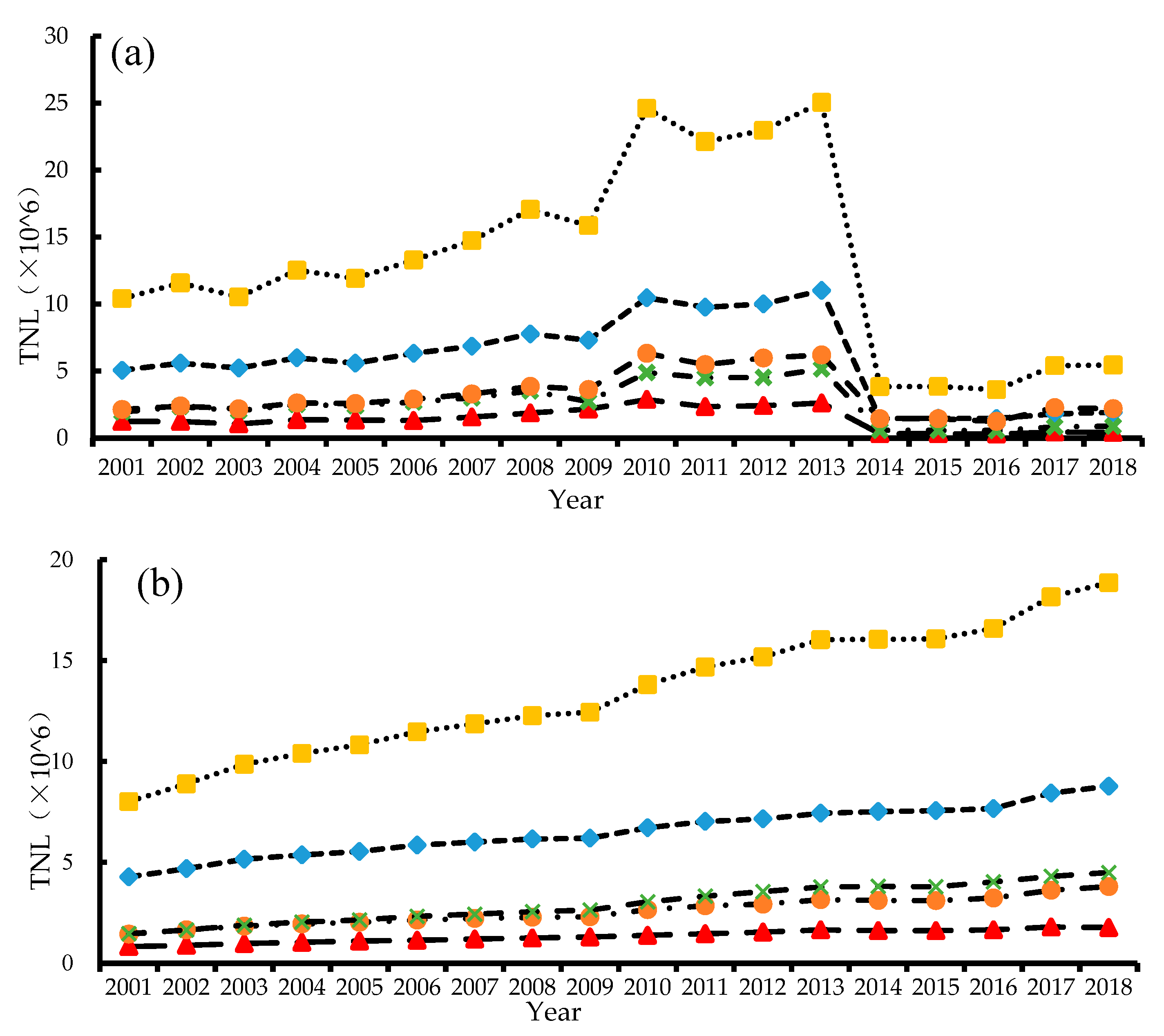
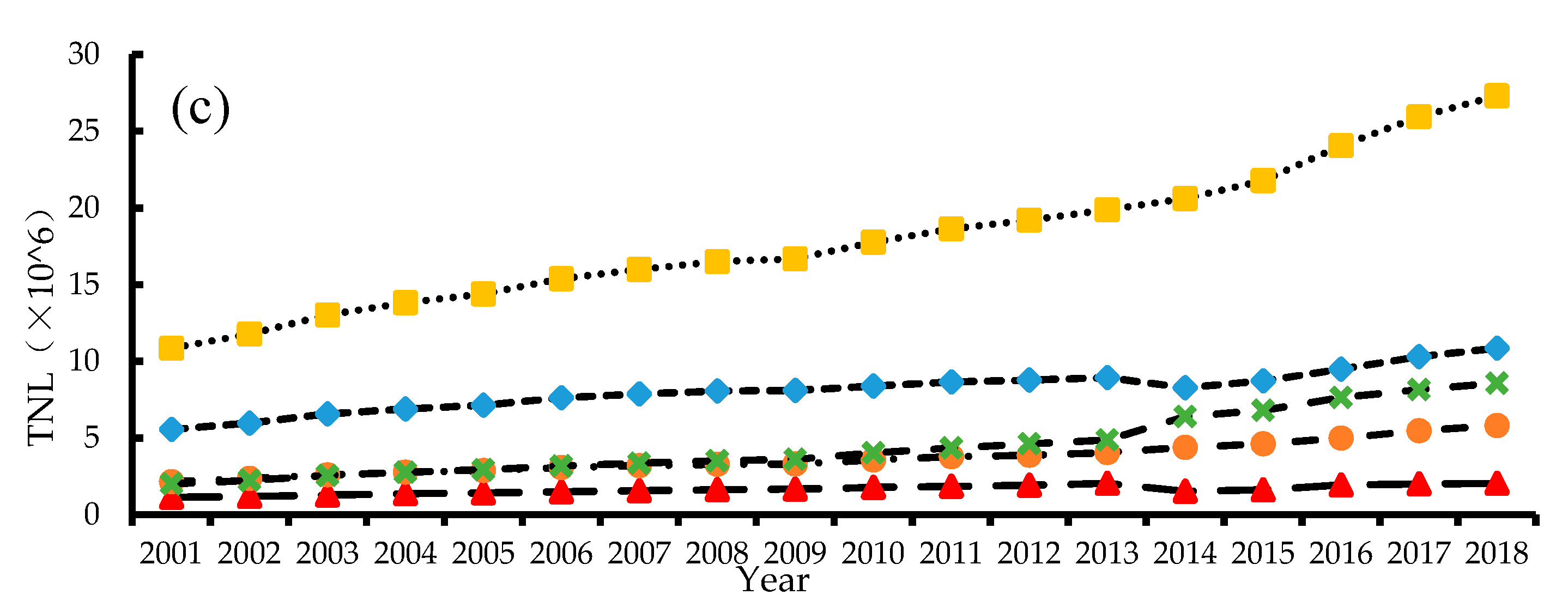
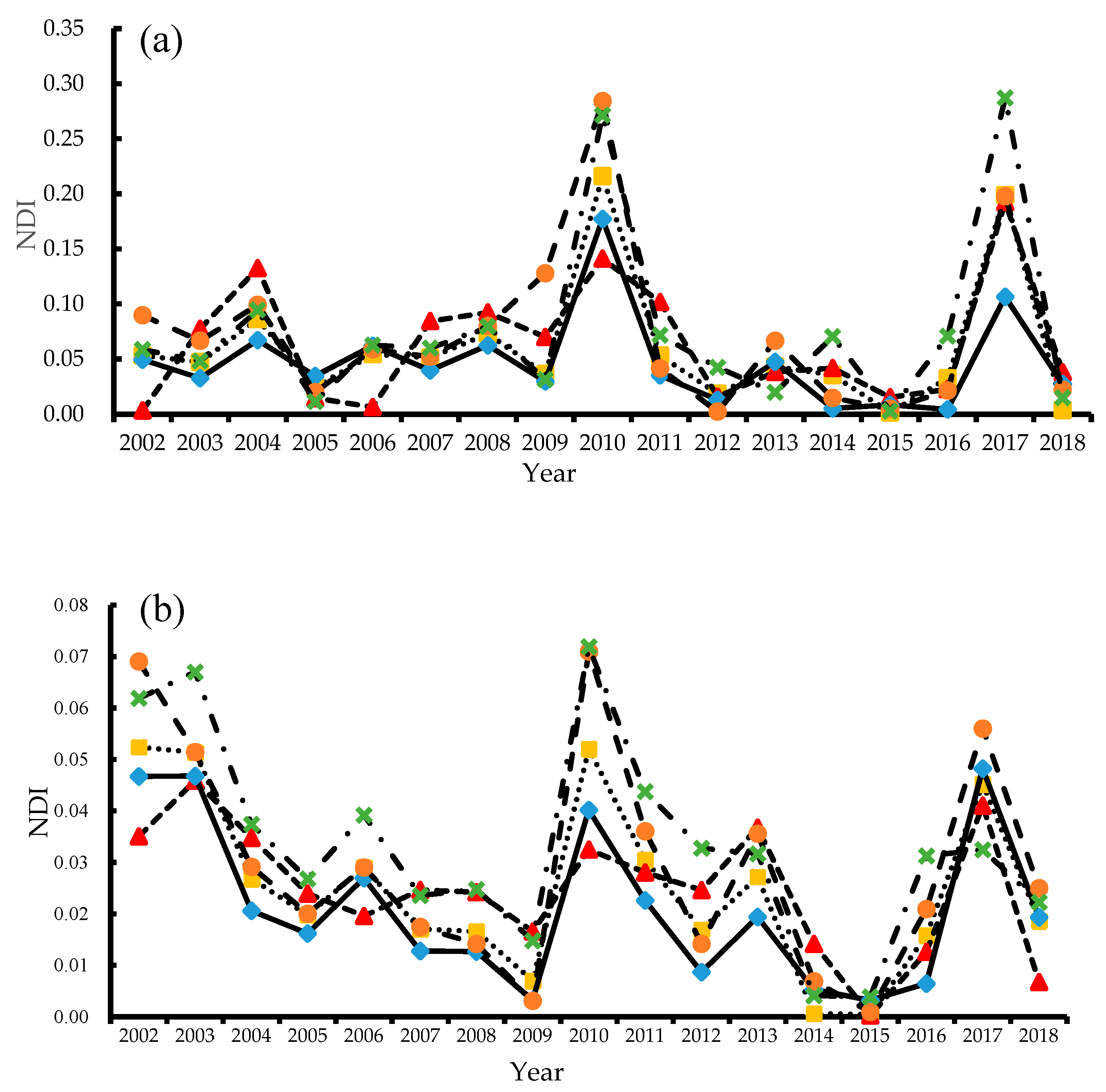
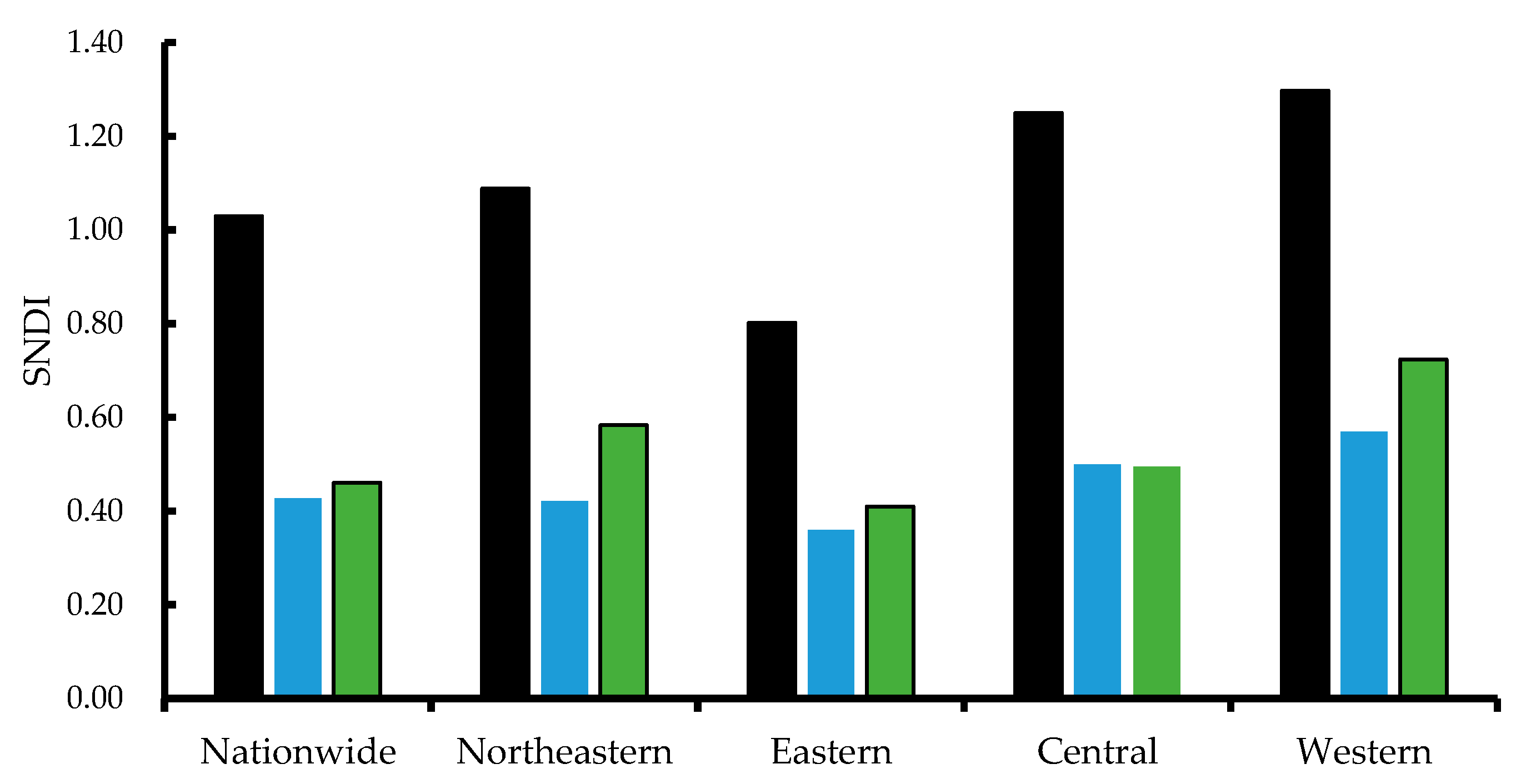
In this paper, 30 provinces in China were divided into four economic regions. Pixel results were compared from economic regions and national scales. In order to illustrate the accuracy of the correction method, night light data before correction and that after correction by the correction method (which was abbreviated as reference correction method below) [63,77] were also compared. The comparison results are shown in Figure 4, Figure 5 and Figure 6. In Figure 4, the abscissa represents different years, the ordinate represents the TNL, and the curve represents the TNL in different years under different treatments. The distribution results of NDI in different regions before and under the two correction methods are compared in Figure 5. SNDI in four economic regions and national scales is compared in Figure 6.

The uncorrected nighttime lighting data fluctuates greatly with the year (Figure 4a). From 2002 to 2003, 2004 to 2005, 2008 to 2009, and 2010 to 2011, the total nighttime lighting shows a downward trend on the national scale, which is inconsistent with the urbanization process in China. On the regional scale, it can be seen that from 2008 to 2009, the northeast region shows the opposite change of the total nighttime lighting with that of the national scale, while the remaining regions show a downward trend of the total nighttime lighting in these years. Moreover, from 2009 to 2010, the total nighttime lighting shows an increase trend, which was also inconsistent with the actual change of nighttime lights. The 2014 NPP/VIIRS data is much smaller in magnitude than the 2013 DMSP/OLS data, which results in the data drop from 2013 to 2014. Although NPP/VIIRS data is obtained from the same satellite, the total nighttime lighting also drops at national and regional scales from 2015 to 2016, and the total nighttime lighting drops at western regions from 2017 to 2018. Therefore, the uncorrected nighttime light data do not reflect the socioeconomic situation in China very well.

As shown in Figure 4b, it can be seen on the national scale from 2001 to 2018, the total nighttime lighting after calibration shows the trend of growth, in accordance with urbanization process in China. However, on the regional scale, from 2013 to 2014 and from 2017 to 2018, the total nighttime lighting in the northeast region decreased. The total nighttime lighting in the central region decreased from 2013 to 2015. Additionally, the total nighttime lighting in the western region decreased from 2014 to 2015. As shown in Figure 4c, it is the change of total nighttime lighting at the national and regional scale after the reference correction method. It can be seen on the national scale from 2001 to 2018, the total nighttime lighting shows the trend of growth, in accordance with urbanization process in China. However, on the regional scale, from 2013 to 2014, the total nighttime lighting in the eastern and northeast regions decreased.

NDI of the nighttime light data (including the DMSP/OLS and NPP/VIIRS data) from 2002 to 2018 were corrected under the correction method in this paper and the reference correction method has improved significantly and the interannual volatility of nighttime lighting data has been greatly reduced (Figure 5). Compared with Figure 5b,c, it can be found that the interannual volatility under the correction method in this paper from 2013 to 2014 is lower than that of reference correction method. Therefore, the difference of nighttime light data within each province should be considered in the regression model of DMSP/OLS data and NPP/VIIRS data. The results of regression fitting for each province are better than those on the national scale.

It can also be seen that no matter the correction method in this paper and reference correction method can all improve the interannual fluctuation of nighttime light data (Figure 6). Before correction, SNDI in northeast, central, western, and national areas are all greater than one except that in the eastern region. After correction, SNDI are about 50% of that before correction. After correcting the nighttime light data with reference correction method, when establishing the regression model of DMSP/OLS and NPP/VIIRS data to fit the NPP/VIIRS data, then fitting the NPP/VIIRS data to the DMSP/OLS data scale in 2014, it will lead to large differences between the correction nighttime light data and DMSP/OLS data in 2013 among some provinces. As a result, the corrected SNDI of the reference correction method on the regional scale is slightly larger than that of the calibration method in this paper. When total nighttime lighting on the national scale is calculated, the influence of the difference in fitting of nighttime light data within the provincial region will be reduced.

4.2. Modeling Results for the Spatiotemporal Dynamics of the Socioeconomic Data

Using the extended temporal coverage nighttime light data, the spatiotemporal dynamics of the GDP from 2001 to 2018 at both the national and provincial scales were modeled. Three regression models were applied: a linear model, a quadratic polynomial model, and a power function model. Then, the best fitting equation was chosen to carry out fitting analysis, compare the fitting accuracy after the correction, and verify the accuracy of the correction algorithm.

4.2.1. Regression Result Analysis at National Scale

Referring to the approach proposed by Zhu et al. [22], through the three regression models mentioned above, the long-term relationships between the corrected TNL and GDP (

Table 1. Accuracy of the estimated statistical gross domestic product (GDP) on time series at the national scale through the three regression models. Note: GDP represents the statistical gross domestic product, PG represents the predicted GDP, RE represents the relative error in percentage, and MARE represents the mean absolute relative error in percentage. The unit of the GDP is billion RMB.

Year	GDP	Linear		Quadratic		Power
		PG	RE (%)	PG	RE (%)	PG	RE (%)
2001	9169.97	−1097.96	−111.97	4777.45	−47.90	7728.93	−15.71
2002	10,174.54	5739.29	−43.59	8992.85	−11.61	10,521.89	3.41
2003	11,870.60	13,176.44	11.00	14,106.73	18.84	14,237.84	19.94
2004	14,199.82	17,379.89	22.40	17,240.72	21.42	16,676.77	17.44
2005	17,587.85	20,625.18	17.27	19,780.70	12.47	18,737.47	6.54
2006	20,630.15	25,625.94	24.22	23,899.95	15.85	22,230.78	7.76
2007	25,089.66	28,699.10	14.39	26,554.94	5.84	24,576.90	−2.04
2008	29,896.13	31,800.50	6.37	29,329.68	−1.89	27,104.57	−9.34
2009	32,983.55	33,141.84	0.48	30,559.41	−7.35	28,248.83	−14.35
2010	39,593.68	43,696.80	10.36	40,861.38	3.20	38,382.57	−3.06
2011	47,291.84	50,403.17	6.58	47,983.41	1.46	45,923.76	−2.89
2012	52,344.84	54,304.79	3.74	52,332.94	−0.02	50,730.02	−3.08
2013	57,714.55	60,868.07	5.46	59,991.69	3.95	59,543.55	3.17
2014	62,397.03	61,031.07	−2.19	60,187.36	−3.54	59,774.41	−4.20
2015	66,111.52	61,139.24	−7.52	60,317.35	−8.76	59,927.91	−9.35
2016	71,582.62	65,132.42	−9.01	65,197.71	−8.92	65,778.80	−8.11
2017	78,154.62	77,271.72	−1.13	81,009.19	3.65	85,851.26	9.85
2018	84,747.64	82,603.11	−2.53	88,417.14	4.33	95,809.71	13.05
MARE (%)	-	-	16.679	-	10.056	-	8.518

), EPC (

Table 2. Accuracy of the estimated statistical electric power consumption (EPC) on time series at the national scale through the three regression models. Note: EPC represents the statistical electric power consumption, PE represents the predicted EPC, RE represents the relative error in percentage, and MARE represents the mean absolute relative error in percentage. The unit of EPC is billion·kilowatt·h⁻¹.

Year	EPC	Linear		Quadratic		Power
		PE	RE (%)	PE	RE (%)	PE	RE (%)
2001	14,678.84	11,309.76	−22.95	11,451.01	−21.99	14,074.76	−4.12
2002	16,382.57	16,049.07	−2.04	16,127.29	−1.56	17,260.43	5.36
2003	18,884.33	21,204.22	12.28	21,226.59	12.40	21,082.72	11.64
2004	21,752.64	24,117.89	10.87	24,114.54	10.86	23,406.88	7.60
2005	24,757.42	26,367.40	6.50	26,347.10	6.42	25,281.90	2.12
2006	28,354.80	29,833.73	5.22	29,792.24	5.07	28,308.34	−0.16
2007	32,550.61	31,963.93	−1.80	31,912.38	−1.96	30,250.55	−7.07
2008	34,333.95	34,113.71	−0.64	34,054.30	−0.81	32,274.01	−6.00
2009	36,577.45	35,043.47	−4.19	34,981.39	−4.36	33,168.84	−9.32
2010	41,978.39	42,359.77	0.91	42,291.60	0.75	40,624.19	−3.23
2011	47,002.11	47,008.36	0.01	46,950.18	−0.11	45,741.46	−2.68
2012	49,563.71	49,712.81	0.30	49,665.41	0.21	48,854.07	−1.43
2013	53,392.76	54,262.23	1.63	54,241.16	1.59	54,314.29	1.73
2014	55,602.70	54,375.22	−2.21	54,354.93	−2.24	54,453.48	−2.07
2015	56,892.45	54,450.19	−4.29	54,430.43	−4.33	54,545.93	−4.12
2016	59,697.87	57,218.11	−4.15	57,219.68	−4.15	58,012.35	−2.82
2017	63,569.00	65,632.61	3.25	65,722.47	3.39	69,186.02	8.84
2018	68,379.00	69,328.13	1.39	69,467.90	1.59	74,394.79	8.80
MARE (%)	-	-	4.702	-	4.655	-	4.950

) in China from 2001 to 2018 were analyzed on time series at the national scale. The R² values obtained from three models between the corrected TNL and GDP are 0.972 (linear), 0.984 (quadratic), and 0.981 (power), respectively, which all represent high correlations and have no marked difference. However, the MARE values vary among the different regression models. For example, the MARE value is 16.679% in the linear model and the MARE value is 10.056% in the quadratic polynomial model, whereas the MARE value is 8.518% in the power function model. This indicates that some details in the relationship between the TNL and GDP may be ignored when the optimal model is selected solely based on the R² values. Thus, these results indicate that all of the three regression models can appropriately reflect the long-term GDP dynamics in China using the nighttime light data from 2001 to 2018 and that the power function model is optimal at the national scale. Moreover, all of the absolute RE values of the power function model employing the extended temporal data are less than or equal to 19.94%.

The R² values obtained from three models between the corrected TNL and EPC are 0.990 (linear), 0.990 (quadratic), and 0.985 (power), respectively, which all represent high correlations and have no marked difference. Moreover, the MARE value is 4.702% in the linear model and the MARE value is 4.655% in the quadratic polynomial model, whereas the MARE value is 4.950% in the power function model. Thus, these results indicate that all of the three regression models can appropriately reflect the long-term EPC dynamics in China and that the quadratic polynomial model is optimal at the national scale. Moreover, all of the absolute RE values of the quadratic polynomial model employing the extended temporal data are less than or equal to 11.64%. Therefore, modeling the long-term dynamics of socioeconomic data in China from 2001 to 2018 using the extended temporal data is reliable.

The predicted GDP and EPC were estimated by the established power function and quadratic polynomial model to further verify the accuracy of GDP modeling (

Table 3. Accuracy of the estimated gross domestic product (GDP) by the established power function on time series at the national scale.

Year	GDP	Corrected in this Article		Reference Correction Method
		PG	RE (%)	PG	RE (%)
2001	9169.97	7728.93	−15.71	8764.45	−40.29
2002	10,174.54	10,521.89	3.41	11,004.77	−32.83
2003	11,870.60	14,237.84	19.94	14,504.52	−23.19
2004	14,199.82	16,676.77	17.44	17,076.50	−21.50
2005	17,587.85	18,737.47	6.54	19,098.76	−22.86
2006	20,630.15	22,230.78	7.76	22,990.08	−18.92
2007	25,089.66	24,576.90	−2.04	25,618.76	−21.30
2008	29,896.13	27,104.57	−9.34	27,983.16	−18.50
2009	32,983.55	28,248.83	−14.35	28,789.82	−21.29
2010	39,593.68	38,382.57	−3.06	34,269.28	−18.36
2011	47,291.84	45,923.76	−2.89	39,158.57	−16.69
2012	52,344.84	50,730.02	−3.08	42,489.26	−14.27
2013	57,714.55	59,543.55	3.17	46,789.37	−12.37
2014	62,397.03	59,774.41	−4.20	51,631.05	−7.14
2015	66,111.52	59,927.91	−9.35	60,203.92	5.82
2016	71,582.62	65,778.80	−8.11	79,240.32	32.74
2017	78,154.62	85,851.26	9.85	97,608.60	53.55
2018	84,747.64	95,809.71	13.05	112,197.69	64.08
MARE (%) before 2013	-	-	8.365	-	21.720
MARE (%) after 2013	-	-	8.913	-	32.666
MARE (%)	-	-	8.518	-	24.761

) and EPC modeling (

Table 4. Accuracy of the estimated statistical electric power consumption (EPC) in time series at the national scale by the established quadratic polynomial model.

Year	EPC	Corrected in this Article		Reference Correction Method
		PE	RE (%)	PE	RE (%)
2001	14,678.84	11,451.01	−21.99	9656.72	−34.21
2002	16,382.57	16,127.29	−1.56	14,605.59	−10.85
2003	18,884.33	21,226.59	12.40	20,880.34	10.57
2004	21,752.64	24,114.54	10.86	24,714.65	13.62
2005	24,757.42	26,347.10	6.42	27,389.91	10.63
2006	28,354.80	29,792.24	5.07	31,891.94	12.47
2007	32,550.61	31,912.38	−1.96	34,551.98	6.15
2008	34,333.95	34,054.30	−0.81	36,733.30	6.99
2009	36,577.45	34,981.39	−4.36	37,437.25	2.35
2010	41,978.39	42,291.60	0.75	41,761.53	−0.52
2011	47,002.11	46,950.18	−0.11	45,067.03	−4.12
2012	49,563.71	49,665.41	0.21	47,080.08	−5.01
2013	53,392.76	54,241.16	1.59	49,440.28	−7.40
2014	55,602.70	54,354.93	−2.24	51,823.81	−6.80
2015	56,892.45	54,430.43	−4.33	55,464.84	−2.51
2016	59,697.87	57,219.68	−4.15	61,620.60	3.22
2017	63,569.00	65,722.47	3.39	65,836.78	3.57
2018	68,379.00	69,467.90	1.59	68,393.99	0.02
MARE (%) before 2013	−	−	5.238	−	9.607
MARE (%) after 2013	−	−	3.141	−	3.223
MARE (%)	−	−	4.655	−	7.834

) based on the time series.

The R² value obtained between the corrected TNL corrected in this paper and GDP is 0.981, whereas the R² value of that corrected under the reference correction method is 0.951. Moreover, the MARE value of the model between the nighttime light data corrected in this paper and GDP is 8.518%, while the MARE of the model between the nighttime light data corrected under the reference correction method and GDP is 24.761% (Table 3). Therefore, the correction method in this paper and the reference correction method can be implemented to GDP on a national scale for dynamic modeling for a long time. Moreover, the calibration method in this paper is slightly better than the reference correction method in modeling accuracy. By comparing the modeling results of nighttime light data before 2013 and that after 2013, it can be found that the MARE of the model between the nighttime light data corrected in this paper and GDP before 2013 is 8.365%, and the MARE of the model between the nighttime light data corrected in this paper and GDP after 2013 is 8.913%. While, the MARE of the model between the nighttime light data corrected under the reference correction method and GDP before 2013 is 21.720%, and the MARE of the model between the nighttime light data corrected under the reference correction method and GDP after 2013 is 32.666%. It can be found that the correction method in this paper has a certain contribution to the saturation correction of DMSP/OLS data compared with the reference correction method, which makes the NTL data better represent GDP.

The R² value obtained between the corrected TNL in this paper and EPC is 0.990, whereas the R² value of that corrected under the reference correction method is 0.976. Moreover, the MARE value of the model between the nighttime light data corrected in this paper and EPC is 4.655%, while the MARE of the model between the nighttime light data corrected under the reference correction method and EPC is 7.834% (Table 4). Therefore, the correction method in this paper and the reference correction method can be implemented to EPC on a national scale for dynamic modeling for a long time. Moreover, the calibration method in this paper is slightly better than the reference correction method in modeling accuracy. By comparing the modeling results of nighttime light data before 2013 and that after 2013, it can be found that the MARE of the model between the nighttime light data corrected in this paper and EPC before 2013 is 5.238%, and the MARE of the model between the nighttime light data corrected in this paper and EPC after 2013 is 3.141%. While the MARE of the model between the nighttime light data corrected under the reference correction method and EPC before 2013 is 9.607%, and the MARE of the model between the nighttime light data corrected under the reference correction method and EPC after 2013 is 3.223%. By comparing Table 3 and Table 4, it can be found that corrected nighttime light data has better modeling ability for EPC (4.655%) on a national scale for dynamic modeling for a long time than for GDP (8.518%), and can be used to predict EPC more accurately.

4.2.2. Regression Result Analysis Based on Provincial Units

The long-term relationships between the corrected TNL and GDP (

Table 5. Model fitting precision values between TNL and GDP in provincial units.

Year	Linear		Quadratic		Power
	R2	MARE (%)	R2	MAPE	R2	MAPE
2001	0.790	55.40	0.791	51.52	0.770	37.30
2002	0.815	50.72	0.815	50.76	0.785	36.17
2003	0.836	46.92	0.836	48.52	0.791	35.72
2004	0.836	45.49	0.837	48.73	0.791	35.97
2005	0.835	41.44	0.845	54.12	0.794	34.64
2006	0.840	39.77	0.851	52.33	0.798	34.28
2007	0.825	41.00	0.838	54.04	0.783	35.11
2008	0.834	40.87	0.849	53.74	0.773	35.65
2009	0.816	44.59	0.834	57.81	0.746	38.28
2010	0.824	42.35	0.845	55.91	0.746	38.01
2011	0.821	43.10	0.842	55.25	0.732	38.42
2012	0.803	45.06	0.828	57.06	0.706	40.25
2013	0.792	45.03	0.820	57.38	0.700	40.63
2014	0.783	46.46	0.812	58.98	0.679	42.01
2015	0.787	45.93	0.817	59.23	0.682	42.38
2016	0.762	46.01	0.808	62.91	0.671	43.12
2017	0.753	47.75	0.796	64.37	0.661	44.29
2018	0.771	46.41	0.800	60.09	0.686	42.54
Average	0.8068	45.239	0.8258	55.708	0.7386	38.599

), EPC (

Table 6. Model fitting precision values between TNL and EPC in provincial units.

Year	Linear		Quadratic		Power
	R2	MARE (%)	R2	MAPE	R2	MAPE
2001	0.889	34.08	0.892	32.04	0.747	30.16
2002	0.902	31.51	0.903	31.04	0.756	30.29
2003	0.895	31.18	0.895	31.40	0.750	31.17
2004	0.896	31.24	0.897	31.10	0.743	31.65
2005	0.896	30.55	0.897	29.86	0.757	30.82
2006	0.893	31.08	0.894	30.57	0.752	31.36
2007	0.890	31.67	0.890	31.20	0.743	32.37
2008	0.890	31.14	0.891	30.35	0.739	32.05
2009	0.885	30.83	0.886	30.05	0.733	32.16
2010	0.888	31.40	0.893	30.31	0.712	33.11
2011	0.884	31.12	0.888	30.41	0.698	33.06
2012	0.880	29.72	0.886	28.70	0.704	31.32
2013	0.871	28.80	0.877	28.16	0.699	30.39
2014	0.878	28.78	0.884	27.93	0.699	30.27
2015	0.890	29.23	0.900	26.82	0.716	30.05
2016	0.893	28.40	0.909	25.57	0.743	28.55
2017	0.881	28.82	0.892	26.83	0.732	29.03
2018	0.889	26.73	0.894	25.39	0.744	27.13
Average	0.8883	30.350	0.8927	29.319	0.7315	30.830

) in China from 2001 to 2018 were analyzed using the three regression models, and the R² and MARE values for each of the three models for each year in provincial units were calculated accordingly. As shown in Table 5, the mean R² values obtained from three models between the corrected TNL and GDP are 0.8068 (linear), 0.8258 (quadratic), and 0.7386 (power), respectively. Moreover, the MARE value is 45.239% in the linear model and the MARE value is 55.708% in the quadratic polynomial model, whereas the MARE value is 38.599% in the power function model. In addition, the MARE value of the power function is lower than that of the other two functions for each year. Therefore, considering the comparison results comprehensively, the power function model was chosen as the fitting function of GDP and TNL.

As shown in Table 6, the mean R² values obtained from three models between the corrected EPC and TNL are 0.8883 (linear), 0.8927 (quadratic), and 0.7315 (power), respectively. Moreover, the MARE value is 30.350% in the linear model and the MARE value is 29.319% in the quadratic polynomial model, whereas the MARE value is 30.830% in the power function model. In addition, the MARE value of the power function is lower than that of the other two functions almost every year. Therefore, considering the comparison results comprehensively, the quadratic polynomial model was chosen as the fitting function of EPC and TNL. It can be seen that the fitting function model in provincial units is the same to that in the national scale.

The relationship between TNL before correction and under two correction methods and GDP and EPC in provincial units in different years was evaluated by power function model (

Table 7. Model fitting precision values between TNL and GDP using power function model in provincial units.

Year	Uncorrected		Corrected		Reference Correction Method
	R2	MARE (%)	R2	MAPE	R2	MAPE
2001	0.725	42.60	0.770	37.30	0.741	40.97
2002	0.762	38.63	0.785	36.17	0.755	39.53
2003	0.786	35.94	0.791	35.72	0.768	37.77
2004	0.766	38.07	0.791	35.97	0.769	37.65
2005	0.758	38.46	0.794	34.64	0.766	36.86
2006	0.771	36.45	0.798	34.28	0.771	36.42
2007	0.765	35.19	0.783	35.11	0.756	37.06
2008	0.719	39.58	0.773	35.65	0.743	37.72
2009	0.644	47.78	0.746	38.28	0.717	40.57
2010	0.602	49.57	0.746	38.01	0.697	42.17
2011	0.652	44.12	0.732	38.42	0.683	42.64
2012	0.600	47.51	0.706	40.25	0.654	44.55
2013	0.630	44.25	0.700	40.63	0.635	45.64
2014	0.311	79.59	0.679	42.01	0.526	50.74
2015	0.301	81.23	0.682	42.38	0.509	52.45
2016	0.417	69.67	0.671	43.12	0.490	53.87
2017	0.165	92.74	0.661	44.29	0.490	54.29
2018	0.225	88.76	0.686	42.54	0.500	53.17
Average	0.5888	52.785	0.7386	38.599	0.6650	43.560

) and quadratic polynomial model (

Table 8. Model fitting precision values between TNL and EPC using quadratic polynomial model in provincial units.

Year	Uncorrected		Corrected		Reference Correction Method
	R2	MARE (%)	R2	MAPE	R2	MAPE
2001	0.845	35.31	0.892	32.04	0.871	34.67
2002	0.869	33.41	0.903	31.04	0.883	33.57
2003	0.888	32.61	0.895	31.40	0.882	33.37
2004	0.871	33.35	0.897	31.10	0.885	32.75
2005	0.867	32.49	0.897	29.86	0.885	31.52
2006	0.878	31.46	0.894	30.57	0.883	31.31
2007	0.890	31.35	0.890	31.20	0.884	31.18
2008	0.884	32.28	0.891	30.35	0.886	30.41
2009	0.778	37.51	0.886	30.05	0.884	30.26
2010	0.822	35.65	0.893	30.31	0.874	30.68
2011	0.877	30.80	0.888	30.41	0.874	30.44
2012	0.876	28.67	0.886	28.70	0.874	28.73
2013	0.867	27.56	0.877	28.16	0.865	28.21
2014	0.654	41.11	0.884	27.93	0.892	25.04
2015	0.639	43.19	0.900	26.82	0.855	26.77
2016	0.712	33.80	0.909	25.57	0.879	25.04
2017	0.561	51.44	0.892	26.83	0.891	24.43
2018	0.591	49.04	0.894	25.39	0.878	24.42
Average	0.7983	35.612	0.8927	29.319	0.8792	29.600

), respectively.

As shown in Table 7, the minimum R² value of the model between TNL of DMSP/OLS images before correction and GDP appeared in 2012, which was 0.600. The maximum R² value of the model between TNL of DMSP/OLS images before correction and GDP appeared in 2003, which was 0.786. However, after 2014, R² value of the model between TNL of NPP/VIIRS images before correction and GDP was lower than 0.5. The minimum R² value appeared in 2017, which was only 0.165. The maximum R² value appeared in 2016, which was only 0.417. The R² values of the model between TNL of NPP/VIIRS annual composite in 2015 and GDP and EPC were 0.792 and 0.834, respectively. Therefore, there were still short-term lights in NPP/VIIRS annual composite images with background noise removed, so the fitting results between TNL and GDP and EPC were worse than those between annual composite images with unstable pixels removed and GDP and EPC.

Under the correction method in this paper, the R² values of the model between TNL and GDP in provincial units were higher than 0.65. The minimum R² value that appeared in 2017 was 0.661. While the maximum R² value that appeared in 2006 was 0.798. The average R² value was 0.7386. The regression result of the correction results under the reference correction method and GDP was also better than the regression result before correction. The minimum R² value that appeared in 2016 and 2017 was 0.490. While the maximum R² value appeared in 2006, which was 0.771. The average R² value was 0.6650. At the same time, the R² and MARE values of the model between TNL of the F162010 radiometric calibration nighttime light image and GDP were 0.795 and 34.97%, the R² and MARE values of that under the correction method were 0.746 and 38.01%, whereas the R² and MARE values of that under the reference correction method were 0.697 and 42.17%. Therefore, it can be found that the correction method in this paper plays a greater role in reducing the “saturation effect” of the image than the reference correction method. By comparing the results of 2015, it can be seen that the R² and MARE values (0.682 and 42.38%) of the model after correction in this paper is lower than that (0.792 and 32.23%) of annual composite image, but better than that (0.509 and 52.45%) corrected under the reference correction method.

As shown in Table 8, under the correction method in this paper, the minimum R² value between TNL after correction in this paper and EPC that appeared in 2013 was 0.877. While the maximum R² value that appeared in 2016 was 0.909. The average R² value was 0.8927. Under the reference correction method, the minimum R² value that appeared in 2015 was 0.855. While the maximum R² value appeared in 2014, which was 0.892. The average R² value was 0.8792. At the same time, the R² and MARE values of the model between TNL of the F162010 radiometric calibration nighttime light image and EPC were 0.861 and 33.36%, the R² and MARE values of that under the correction method were 0.893 and 30.31%, whereas the R² and MARE values of that under the reference correction method were 0.874 and 30.68%. Therefore, it can be also found that the correction method in this paper plays a greater role in reducing the “saturation effect” of the image than the reference correction method. By comparing the results of 2015, it can be seen that the R² and MARE values (0.900 and 26.82%) after correction in this paper is better than that (0.855 and 26.77%) corrected under the reference correction method, and better than that (0.834 and 29.96%) of the annual composite image.

By comparing the relationship between TNL and EPC under different treatments, it can also be found that the regression results under the correction method introduced in this paper are better than those under the reference correction method, and the regression results under two correction methods are all better than the regression results before the correction. Therefore, the nighttime light data corrected by the correction method in this paper can reflect GDP and EPC better than in provincial units than that corrected under the reference correction method and that before correction.

4.2.3. Regression Result Analysis Based on Time Series

The long-term relationships between the corrected TNL and GDP (

Table 9. Model fitting precision values between TNL and GDP in time series.

Year	Linear		Quadratic		Power
	R2	MARE (%)	R2	MAPE	R2	MAPE
Anhui	0.972	16.02	0.988	8.36	0.983	8.04
Beijing	0.966	18.46	0.974	12.68	0.964	12.41
Chongqing	0.961	26.48	0.966	21.22	0.957	15.98
Fujian	0.953	17.38	0.985	5.12	0.992	5.23
Gansu	0.991	8.31	0.991	8.28	0.969	9.73
Guangdong	0.945	17.86	0.947	15.46	0.939	13.44
Guangxi	0.975	18.87	0.976	17.21	0.972	11.28
Guizhou	0.973	24.83	0.976	20.21	0.958	15.85
Hainan	0.894	25.02	0.927	12.04	0.966	12.53
Hebei	0.951	15.70	0.951	15.60	0.957	11.91
Heilongjiang	0.972	7.58	0.973	6.83	0.982	5.23
Henan	0.934	23.79	0.956	13.77	0.966	10.94
Hubei	0.976	13.54	0.978	11.86	0.969	10.97
Hunan	0.981	17.79	0.981	17.79	0.949	15.15
Inner Mongolia	0.957	24.11	0.959	19.65	0.976	11.99
Jiangsu	0.927	28.60	0.985	8.20	0.959	10.98
Jiangxi	0.959	26.04	0.961	23.58	0.941	16.82
Jilin	0.966	18.15	0.966	16.78	0.969	11.92
Liaoning	0.900	15.72	0.902	17.07	0.949	12.50
Ningxia	0.957	28.68	0.982	12.85	0.977	10.45
Qinghai	0.985	12.84	0.986	11.67	0.984	8.70
Shaanxi	0.926	32.97	0.976	7.83	0.981	10.42
Shandong	0.929	21.92	0.933	18.53	0.955	13.14
Shanghai	0.937	14.59	0.959	9.00	0.966	9.31
Shanxi	0.931	21.98	0.955	12.05	0.970	10.87
Sichuan	0.937	26.21	0.958	15.73	0.960	12.39
Tianjin	0.931	30.95	0.962	15.16	0.974	11.57
Xinjiang	0.991	5.28	0.992	5.12	0.988	5.91
Yunnan	0.945	19.55	0.978	6.68	0.984	7.27
Zhejiang	0.966	17.27	0.970	14.47	0.956	12.49
Average	0.9529	19.883	0.9664	13.361	0.9671	11.181

), EPC (

Table 10. Model fitting precision values between TNL and EPC in time series.

Year	Linear		Quadratic		Power
	R2	MARE (%)	R2	MAPE	R2	MAPE
Anhui	0.985	6.62	0.987	6.32	0.982	6.03
Beijing	0.982	3.43	0.983	3.63	0.980	3.64
Chongqing	0.972	8.57	0.973	8.81	0.963	8.40
Fujian	0.992	2.82	0.993	2.74	0.988	4.78
Gansu	0.978	6.59	0.990	4.14	0.970	6.20
Guangdong	0.960	5.42	0.967	5.70	0.945	8.29
Guangxi	0.972	7.84	0.975	8.54	0.973	7.06
Guizhou	0.960	8.85	0.975	7.87	0.951	9.09
Hainan	0.923	14.71	0.936	10.72	0.965	10.78
Hebei	0.930	9.39	0.953	10.21	0.932	10.30
Heilongjiang	0.980	2.54	0.980	2.53	0.981	2.65
Henan	0.961	8.06	0.963	8.24	0.965	7.69
Hubei	0.964	7.94	0.980	5.52	0.944	8.02
Hunan	0.929	10.70	0.968	7.73	0.924	10.28
Inner Mongolia	0.911	18.45	0.926	9.77	0.976	9.73
Jiangsu	0.978	8.59	0.983	7.71	0.971	6.98
Jiangxi	0.973	10.59	0.973	10.38	0.958	9.50
Jilin	0.959	4.66	0.972	4.33	0.967	4.68
Liaoning	0.992	2.47	0.993	2.55	0.990	2.97
Ningxia	0.978	9.25	0.983	6.00	0.989	4.97
Qinghai	0.959	9.35	0.972	11.86	0.972	8.62
Shaanxi	0.950	9.38	0.976	5.05	0.980	5.71
Shandong	0.933	11.48	0.934	10.16	0.961	7.84
Shanghai	0.967	4.59	0.977	4.12	0.963	4.88
Shanxi	0.965	6.49	0.967	5.76	0.973	5.31
Sichuan	0.979	5.72	0.979	5.79	0.979	5.65
Tianjin	0.962	6.74	0.963	7.08	0.971	5.90
Xinjiang	0.936	27.47	0.961	8.60	0.981	10.12
Yunnan	0.985	6.53	0.985	6.79	0.978	6.60
Zhejiang	0.968	8.81	0.971	8.80	0.952	9.33
Average	0.9628	8.468	0.9713	6.915	0.9675	7.066

) in China from 2001 to 2018 were analyzed using the three regression models, and the R² and MARE values for each of the three models for each province were calculated accordingly. As shown in Table 9, the mean R² values obtained from three models between the corrected TNL and GDP are 0.9529 (linear), 0.9664 (quadratic), and 0.9671 (power), respectively. Furthermore, the R² values of the three models are similar among most of the provinces, whereas the MARE values vary substantially with the different models for each province. It can be concluded that at the provincial level, all of the three models are reliable for modeling the long-term GDP dynamics the nighttime light data from 2001 to 2018. In general, the power function model is the best-fitting model, with the minimum mean MARE value of 11.181%, whereas the MARE value is 19.883% in the linear model and the MARE value is 13.361% in the quadratic polynomial model, which is supported by previous studies [13,22,78].

As shown in Table 10, the mean R² values obtained from three models between the corrected EPC and TNL are 0.9628 (linear), 0.9713 (quadratic), and 0.9675 (power), respectively. Moreover, the MARE value is 8.468% in the linear model and the MARE value is 6.915% in the quadratic polynomial model, whereas the MARE value is 7.066% in the power function model. It can be seen that the fitting function model for each province is the same as that in provincial units and the national scale.

To further ascertain the most effective model for each province, the optimal models were chosen through a comparison of the R² and MARE values of each model. The quadratic polynomial model is found to be optimal in eight provinces (Fujian, Gansu, Hainan, Jiangsu, Shaanxi, Shanghai, Xinjiang, and Yunnan) while the power function model is optimal for modeling the dynamics of the GDP from 2001 to 2018 for the remaining provinces. The quadratic polynomial model is found to be optimal in 12 provinces (Fujian, Gansu, Guizhou, Hainan, Heilongjiang, Hubei, Hunan, Jilin, Shaanxi, Shanghai, Xinjiang, Zhejiang), the linear model is optimal in five provinces (Beijing, Guangdong, Hebei, Liaoning, and Yunnan) while the power function model is optimal for modeling the dynamics of the EPC from 2001 to 2018 for the remaining provinces.

Consequently, although the power function model and quadratic polynomial model is generally the best-fitting model for long-term modeling of GDP and EPC dynamics using the nighttime light data from 2001 to 2018 for each province in time series, the optimal model varies for different provinces of China. The relationship between TNL before correction and under two correction methods and GDP and EPC in provincial units in different years was evaluated by the corresponding best-fitting model, respectively.

Referring to the method proposed by Shi et al. [61], the minimum R² value of the model between TNL corrected in this paper and GDP was 0.927, the maximum R² value was 0.992, and the average R² value was 0.9667 (

Table 11. R² values and F-tests of the regression analyses for prefectural units of each province. Note: Y represents the regression equation has passed the F-test at the 0.001 level, N represents the regression equation has not passed the test.

Provincial-Level Units	TNL and GDP				TNL and EPC
	Corrected		Reference Correction Method		Corrected		Reference Correction Method
	R2	F-Test	R2	F-Test	R2	F-Test	R2	F-Test
Anhui	0.983	Y	0.965	Y	0.982	Y	0.961	Y
Beijing	0.964	Y	0.458	Y	0.982	Y	0.477	Y
Chongqing	0.957	Y	0.889	Y	0.963	Y	0.883	Y
Fujian	0.985	Y	0.970	Y	0.993	Y	0.971	Y
Gansu	0.991	Y	0.969	Y	0.990	Y	0.950	Y
Guangdong	0.939	Y	0.902	Y	0.960	Y	0.888	Y
Guangxi	0.972	Y	0.933	Y	0.973	Y	0.926	Y
Guizhou	0.958	Y	0.828	Y	0.975	Y	0.854	Y
Hainan	0.927	Y	0.982	Y	0.936	Y	0.981	Y
Hebei	0.957	Y	0.812	Y	0.930	Y	0.772	Y
Heilongjiang	0.982	Y	0.633	Y	0.980	Y	0.579	Y
Henan	0.966	Y	0.886	Y	0.965	Y	0.905	Y
Hubei	0.969	Y	0.948	Y	0.980	Y	0.968	Y
Hunan	0.949	Y	0.852	Y	0.968	Y	0.887	Y
Inner Mongolia	0.976	Y	0.950	Y	0.976	Y	0.977	Y
Jiangsu	0.985	Y	0.937	Y	0.971	Y	0.953	Y
Jiangxi	0.941	Y	0.884	Y	0.958	Y	0.906	Y
Jilin	0.969	Y	0.914	Y	0.972	Y	0.952	Y
Liaoning	0.949	Y	0.774	Y	0.992	Y	0.840	Y
Ningxia	0.977	Y	0.923	Y	0.989	Y	0.928	Y
Qinghai	0.984	Y	0.803	Y	0.972	Y	0.743	Y
Shaanxi	0.976	Y	0.975	Y	0.976	Y	0.988	Y
Shandong	0.955	Y	0.301	N	0.961	Y	0.292	N
Shanghai	0.959	Y	0.884	Y	0.977	Y	0.861	Y
Shanxi	0.970	Y	0.910	Y	0.973	Y	0.912	Y
Sichuan	0.960	Y	0.837	Y	0.979	Y	0.801	Y
Tianjin	0.974	Y	0.001	N	0.971	Y	0.001	N
Xinjiang	0.992	Y	0.983	Y	0.961	Y	0.943	Y
Yunnan	0.978	Y	0.970	Y	0.985	Y	0.834	Y
Zhejiang	0.956	Y	0.901	Y	0.971	Y	0.925	Y
Average	0.9667	-	0.8325	-	0.9720	-	0.8286	-

). According to the reference correction method, the minimum R² value of the model between TNL corrected and GDP was only 0.001, the maximum R² value was 0.983, and the average R² value was 0.8325. Besides, the minimum R² value of the model between TNL corrected in this paper and EPC was 0.930, the maximum R² value was 0.993, and the average R² value was 0.9720. According to the reference correction method, the minimum R² value of the model between TNL corrected and EPC was only 0.001, the maximum R² value was 0.988 and the average R² value was 0.8286. In addition, the TNL-GDP model and TNL-EPC model of 30 provinces obtained in this paper have all passed the F-test at the level of 0.001, while the TNL-GDP model and TNL-EPC model of 28 provinces besides Tianjin and Shandong obtained under the reference correction method passed the F-test at the level of 0.001.

Furthermore, the MARE value of the predicted GDP (

Table 12. MARE of the predicted gross domestic product (GDP) in time series and in provincial units.

Provincial-Level Units	Modeling in Time Series		Modeling in Provincial Units
	Corrected	Reference Correction Method	Uncorrected	Corrected	Reference Correction Method
Anhui	8.04	12.22	13.55	8.75	9.20
Beijing	12.41	39.12	54.28	43.95	56.07
Chongqing	15.98	23.76	42.39	48.76	44.40
Fujian	5.12	12.72	20.65	18.15	17.57
Gansu	8.28	11.19	77.24	41.35	67.16
Guangdong	13.44	15.98	28.13	14.38	22.43
Guangxi	11.28	16.11	20.95	20.26	24.90
Guizhou	15.85	31.78	20.54	5.06	25.42
Hainan	12.04	15.39	117.03	114.41	113.43
Hebei	11.91	17.42	25.68	36.54	28.79
Heilongjiang	5.23	22.26	61.97	68.64	43.61
Henan	10.94	17.14	18.63	11.95	17.13
Hubei	10.97	14.43	35.47	40.49	37.95
Hunan	15.15	25.81	40.61	47.92	39.84
Inner Mongolia	11.99	16.11	48.73	32.53	24.91
Jiangsu	8.20	21.26	31.78	18.22	24.63
Jiangxi	16.82	22.65	23.77	27.16	17.47
Jilin	11.92	17.92	17.63	5.79	6.37
Liaoning	12.50	17.33	15.29	14.04	16.06
Ningxia	10.45	22.16	100.43	93.06	97.24
Qinghai	8.70	29.58	210.44	15.61	65.63
Shaanxi	7.83	18.87	27.20	29.13	37.33
Shandong	13.14	-	22.08	5.94	15.13
Shanghai	9.00	18.87	64.52	61.95	66.24
Shanxi	10.87	14.07	70.57	91.02	106.54
Sichuan	12.39	25.82	23.94	30.49	21.98
Tianjin	11.57	-	40.07	30.30	43.44
Xinjiang	5.12	7.55	209.99	94.42	115.76
Yunnan	6.68	13.32	66.57	63.68	74.50
Zhejiang	12.49	18.13	33.41	24.03	25.65
Average	10.877	19.249	52.785	38.599	43.560

) and the predicted EPC (

Table 13. MARE of the predicted electric power consumption (EPC) in time series and in provincial units.

Provincial-Level Units	Modeling in Time Series		Modeling in Provincial Units
	Corrected	Reference Correction Method	Uncorrected	Corrected	Reference Correction Method
Anhui	6.03	9.49	20.49	19.14	16.86
Beijing	3.43	17.59	13.80	14.38	10.56
Chongqing	8.40	14.34	13.98	9.08	3.45
Fujian	2.74	6.49	10.66	8.29	5.63
Gansu	4.14	7.02	22.54	17.46	13.07
Guangdong	5.42	10.56	11.95	8.54	5.91
Guangxi	7.06	11.61	15.82	16.64	14.62
Guizhou	7.87	15.50	20.10	29.63	21.50
Hainan	10.72	10.35	237.36	235.29	255.36
Hebei	9.39	14.09	10.29	10.54	7.21
Heilongjiang	2.53	12.78	121.94	110.88	77.58
Henan	7.69	10.24	8.30	7.42	3.34
Hubei	5.52	6.44	15.91	24.38	21.89
Hunan	7.73	11.61	16.12	24.42	18.94
Inner Mongolia	9.73	8.80	20.73	23.40	24.07
Jiangsu	6.98	9.50	16.10	13.94	10.44
Jiangxi	9.50	14.45	20.65	11.31	15.59
Jilin	4.33	5.52	67.37	60.35	45.35
Liaoning	2.47	7.71	11.44	12.66	18.36
Ningxia	4.97	14.25	33.52	16.87	12.26
Qinghai	8.62	26.49	67.26	14.46	13.64
Shaanxi	5.05	4.73	43.18	40.65	45.19
Shandong	7.84	-	21.70	16.97	19.97
Shanghai	4.12	8.73	37.12	36.55	41.51
Shanxi	5.31	8.19	7.89	12.94	15.53
Sichuan	5.65	16.32	28.04	27.67	30.37
Tianjin	5.90	-	14.59	27.34	15.60
Xinjiang	8.60	24.65	83.07	43.06	54.35
Yunnan	6.53	20.46	31.97	23.73	29.50
Zhejiang	8.80	13.07	24.48	26.63	20.35
Average	6.435	12.178	35.612	31.487	29.600

) in time series and in provincial units under the two correction methods was further analyzed. When modeling based on time series, MARE values of the predicted GDP under the corrected NTL data in this paper are 16.82% (Jiangxi) and 5.12% (Xinjiang), while MARE values of the predicted GDP under that of the reference correction method are 39.12% (Beijing) and 7.55% (Xinjiang) (Table 12). The correction method in this paper is better than the reference correction method in estimating the GDP of specific provincial units. For the provincial units, the MARE values of the uncorrected nighttime light data in predicting the GDP of Qinghai and Anhui are 210.44% and 13.55%. At the same time, MARE values of the predicted GDP under the corrected nighttime light data in this paper are 114.41% (Hainan) and 5.06% (Guizhou), while MARE values predicted GDP under that of the reference correction method are 115.76% (Xinjiang) and 6.37% (Jilin). Therefore, the performance prediction GDP under nighttime light data processed by the two correction methods is better than that before correction. When forecasting GDP of Hainan, Ningxia, Qinghai, and Xinjiang based on the model on provincial unit, MAREs are all large under two correction methods and before correction because it is difficult to distinguish the real lights in urbanization areas from other artificial structures or some special surface reflected lights.

Based on the model of nighttime light data and GDP established by time series, the MARE value under the correction method in this paper is 10.877%, while the MARE value under the reference correction method is 19.249%. It is shown that the correction method in this paper is also better than the reference correction method in the long-term dynamic modeling of GDP on the provincial scale. Based on the model of nighttime light data and GDP established by provincial units, the MARE value under the correction method in this paper is 38.599%, the MARE value under the reference correction method is 43.560%, while the MARE before correction is 52.785%. The MARE value of the model based on provincial units under the two correction methods is far greater than that based on time series. When modeling in provincial units, the nighttime light data of some provincial units are not real data, so the correlation between nighttime light data and GDP will be reduced during modeling, thus reducing the accuracy of GDP prediction. When modeling in time series, it is not necessary to consider the differences in this part. Therefore, when predicting the GDP of specific provincial units, the regression model based on time series is preferred.

The MARE value of the model between the nighttime light data under the correction method in this paper and EPC based on time series is 6.435%, while the MARE value under the reference correction method is 12.178% (Table 13). It is shown that the ability of predicting EPC for dynamic modeling for a long time in the provincial scale under the correction method in this paper is better than that under the reference correction method. Based on the model of nighttime light data and EPC established by provincial units, the MARE value under the calibration method in this paper is 31.487%, the MARE value under the reference correction method is 29.600%, while the MARE value before the calibration is 35.612%. The MARE value based on the modeling of provincial units under the two correction methods is also much greater than that based on the modeling of time series. Therefore, when predicting the EPC of specific provincial units, the regression model based on time series is also optimized.

The MARE value is further divided into three categories [61]: 0–25% is high accuracy, 25–50% is medium accuracy, and more than 50% is inaccuracy (

Table 14. Different classes of predicted accuracies for GDP and EPC under three data process methods.

	Model Classification	Data Processing Method	Percentage of MARE (%)
			High Accuracy	Moderate Accuracy	Inaccuracy
TNL and GDP	Modeling in time series	Corrected	100.00	0	0
		Reference correction method	76.67	16.67	6.67
	Modeling in provincial units	Uncorrected	33.33	33.33	33.33
		Corrected	40.00	36.67	23.33
		Reference correction method	40.00	30.00	30.00
TNL and EPC	Modeling in time series	Corrected	100.00	0	0
		Reference correction method	90.00	3.33	6.67
	Modeling in provincial units	Uncorrected	66.67	16.67	16.67
		Corrected	66.67	23.33	10.00
		Reference correction method	73.33	16.67	10.00

).

In the TNL-GDP and TNL-EPC models established based on time series, the correction method introduced in this paper has extremely significant prediction ability with prediction accuracy of 100%, which is higher than the prediction accuracy (76.67% and 90.00%) of the reference correction method. The prediction inaccuracy in this paper is also less than the prediction inaccuracy (6.67% and 6.67%) of the reference correction method. Compared with the prediction ability of GDP and EPC under the correction method introduced in this paper and the reference correction method, it can be found that the ability of the correction method introduced in this paper in the prediction of GDP and EPC is also better than that of the reference correction method.

5. Discussion

DMSP/OLS data and NPP/VIIRS data are the most widely used to obtain the nighttime light data for monitoring human socioeconomic activities and natural phenomena [6]. Light saturation in the city center, blooming effect, and lack of airborne calibration are the major obstacles to the application of DMSP/OLS data. In addition, when building a long time series of nighttime light datasets, the inconsistency between NPP/VIIRS data and DMSP/OLS data is more serious than that between the different products of the DMSP/OLS data [50]. Although, scholars have done a lot of research on the processing of DMSP/OLS Data and NPP/VIIRS data, but there are still some limitations in the existing research results.

Aiming at the problems in the current research, this paper proposes the WorldPop and the enhanced vegetation index adjusted nighttime light (WEANTL) using EVI and WorldPop data based on the principle that urban characteristics (including nighttime light) should be inversely proportional to vegetation coverage [38] and directly proportional to population distribution data [53,54], so as to obtain the nighttime light dataset from 2001 to 2018 to represent economic data reliably and accurately. The result shows that the extended nighttime light data set has good quality and reliable time consistency. Considering that the use of nighttime light data to reflect social and economic development is carried out by constructing the statistical relationship between TNL and socioeconomic parameters [7,9,35,74,75], this paper also evaluates the accuracy of the correction method proposed in this paper in predicting socioeconomic parameters by constructing a regression model between TNL and socioeconomic parameters.

In the saturation correction of DMSP/OLS data, the existing research did not distinguish the spatial differences of the saturated pixels and carried out the saturation correction of the unsaturated pixels, thus failed to effectively correct the saturation of the DMSP/OLS data. When fitting DMSP/OLS data and NPP/VIIRS data, some scholars used the same fitting function to fit the data of 30 provinces, without considering the data differences of each province, thus reducing the ability of night light data to represent economic data. Compared with the previous models [63,77], it can effectively distinguish the spatial differences of the nighttime light data because EVI and WorldPop data was used to realize the saturation correction of DMSP/OLS data.

In this paper, when fitting DMSP/OLS data and NPP/VIIRS data, considering the differences of economic development of each province, linear regression models were developed for each province. It can be seen from the above paper, the TNL-GDP model and TNL-EPC model of 30 provinces obtained in this paper all passed the F-test at the level of 0.001, while the TNL-GDP model and TNL-EPC model of 28 provinces besides Tianjin and Shandong obtained under the reference correction method passed the F-test at the level of 0.001. Tianjin and Shandong failed to pass the F-test mainly because when fitting DMSP/OLS and NPP/VIIRS data, the model was fitted on all county-level scales in China in 2012 and 2013. NPP/VIIRS data from 2014 to 2018 were fitted to DMSP/OLS data according to the fitting model, which can ensure that the DMSP/OLS data in later years after fitting on a national scale is almost larger than that in previous years. However, there is no guarantee that DMSP/OLS data in later years after fitting of all the provincial units in the provincial scale is greater than the DMSP/OLS data in previous years. For example, the DMSP/OLS data of Beijing in 2014 or 2015 after fitting is less than that in 2013, leading to the R² values of the TNL-GDP model and TNL-EPC model being below the average. The DMSP/OLS data of Tianjin and Shandong after fitting from 2014 to 2018 is all less than that in 2013. As a result, the established regression model could not pass the F test at the 0.001 level. Therefore, it is necessary to establish the fitting equation between the DMSP/OLS and NPP/VIIRS data in 2012 and 2013 for the specific research area when studying the research area on and below the provincial scale.

Compared with the existing research, the main contributions of this paper are as follows: (1) DMSP/OLS image is divided into saturation and unsaturated regions, WEANTL was put forward to correct the image data in the saturation region by using EVI and WorldPop data of the corresponding year, and pixel points in the unsaturated region kept the original value. Therefore, the saturation correction of DMSP/OLS image data from 2001 to 2013 is realized by using EVI and WorldPop data. (2) The unstable pixels in 2012–2015 and 2015–2018 NPP/VIIRS annual images are removed by the annual night light images of NPP/VIIRS in 2015 and 2016, respectively, which retain more effective information than previous studies. (3) The total nighttime lights on the county scale of 30 provinces is calculated. The regression model carried out the regression analysis on the total nighttime lights of DMSP/OLS data and NPP/VIIRS data in 2012 and 2013, respectively. Compared with previous studies, it can better fit and correct night light data and economic data on a provincial scale.

As a correction method for fitting DMSP/OLS data and NPP/VIIRS data to obtain a long time series of nighttime light data sets for continuous monitoring of society, this method has made some contributions, but there are still some limitations. Firstly, although the prediction accuracy of the proposed correction method in establishing long-term GDP and EPC dynamic models is better than that of the reference correction method, the saturation problem in the DMSP/OLS data and the noise data in NPP/VIIRS data are not removed completely. These problems reduce the accuracy of long time series nighttime light datasets and the prediction accuracy of establishing long-term GDP and EPC dynamic models. Secondly, considering that regression models (quadratic polynomial model and power function model) have been applied in this paper to model socioeconomic activities using nighttime light data, more complex models need to be developed to predict socioeconomic activities more accurately. Therefore, with the updating of NPP/VIIRS data and more sources of nighttime light data, such as luojia1-01 satellite, new methods for multisensor nighttime light data to model social and economic dynamic situations can be developed in future research.

6. Conclusions

This paper proposes an invariant region method based on EVI and WorldPop data to achieve intercalibration and saturation correction of DMSP/OLS data, and uses a regression model to achieve the fitting of DMSP/OLS data and NPP/VIIRS data, and constructs a long time series of night light images from 2001 to 2018. Comparing the pixel results processed by three data processing methods (uncorrected, calibration method introduced in this paper and the reference correction method), the ability to estimate GDP and EPC based on time series on the national scale and the ability to estimate GDP and EPC based on time series and on provincial units under two correction methods (calibration method introduced in this paper and the reference correction method) were carried out.

In this research, we found that (1) after calibration, the NTL data can guarantee the growth trend on national and regional scales, and the interannual volatility of the corrected NTL data is lower than that of the uncorrected NTL data; (2) on the national scale, compared with the established model of NTL-GDP, the R² and the MARE are 0.981 and 8.518%. The R² and MARE of the established model of NTL data and EPC data (NTL-EPC) are 0.990 and 4.655%; (3) on the provincial scale, the R² and MARE of NTL-GDP model under the provincial units are 0.7386 and 38.599%. The R² value and MARE of NTL-EPC model are 0.8927 and 29.319%; (4) on the provincial scale, the R² and MARE of NTL-GDP model on time series are 0.9667 and 10.877%. The R² and MARE of NTL-GDP model on time series are 0.9720 and 6.435%; the established TNL-GDP and TNL-EPC models with 30 provinces data all passed the F-test at the 0.001 level; (5) the prediction accuracy of GDP and EPC on time series was nearly 100%. Therefore, the correction method in this paper can reliably and accurately estimate GDP and EPC on multiple scales.

References

- Li, D.; Li, X. An Overview on Data Mining of Nighttime Light Remote Sensing. Acta Geod. Cartogr. Sinica. 2015, 6, 591–601. [Google Scholar] [CrossRef]
- Jiang, W.; He, G.; Peng, Y.; Wang, G.; Wang, M. Application potentiality and prospects of nighttime light remote sensing in “the Belt and Road” initiative. J. Univ. Chin. Acad. Sci. 2017, 3, 296–303. [Google Scholar] [CrossRef]
- Kiyofuji, H.; Saitoh, S. Use of nighttime visible images to detect Japanese common squid Todarodes pacificus fishing areas and potential migration routes in the Sea of Japan. Mar. Ecol. Prog. Ser. 2004, 276, 173–186. [Google Scholar] [CrossRef]
- Elvidge, C.D.; Ziskin, D.; Baugh, K.E.; Tuttle, B.T.; Ghosh, T.; Pack, D.W.; Erwin, E.H.; Zhizhin, M. A Fifteen Year Record of Global Natural Gas Flaring Derived from Satellite Data. Energies 2009, 2, 595–622. [Google Scholar] [CrossRef]
- Chand, T.R.K.; Badarinath, K.V.S.; Murthy, M.S.R.; Rajshekhar, G.; Elvidge, C.D.; Tuttle, B.T. Active forest fire monitoring in Uttaranchal State, India using multi-temporal DMSP-OLS and MODIS data. Int. J. Remote Sens. 2007, 28, 2123–2132. [Google Scholar] [CrossRef]
- Elvidge, C.D.; Erwin, E.H.; Baugh, K.E.; Ziskin, D.; Tuttle, B.T.; Ghosh, T.; Sutton, P.C. Overview of DMSP nightime lights and future possibilities. In Proceedings of the 2009 Joint Urban Remote Sensing Event, Shanghai, China, 20–22 May 2009; pp. 1–5. [Google Scholar]
- Liang, H.; Guo, Z.; Wu, J.; Chen, Z. GDP spatialization in Ningbo City based on NPP/VIIRS night-time light and auxiliary data using random forest regression. Adv. Space Res. 2020, 65, 481–493. [Google Scholar] [CrossRef]
- Tan, M.; Li, X.; Li, S.; Xin, L.; Wang, X.; Li, Q.; Li, W.; Li, Y.; Xiang, W. Modeling population density based on nighttime light images and land use data in China. Appl. Energy 2018, 90, 239–247. [Google Scholar] [CrossRef]
- Hu, T.; Huang, X. A novel locally adaptive method for modeling the spatiotemporal dynamics of global electric power consumption based on DMSP-OLS nighttime stable light data. Appl. Energy 2019, 240, 778–792. [Google Scholar] [CrossRef]
- Wang, S.; Shi, C.; Fang, C.; Feng, K. Examining the spatial variations of determinants of energy-related CO2 emissions in China at the city level using Geographically Weighted Regression Model. Appl. Energy 2019, 235, 95–105. [Google Scholar] [CrossRef]
- Wang, W.; Cheng, H.; Zhang, L. Poverty assessment using DMSP/OLS night-time light satellite imagery at a provincial scale in China. Adv. Space Res. 2012, 49, 1253–1264. [Google Scholar] [CrossRef]
- Small, C.; Pozzi, F.; Elvidge, C.D. Spatial analysis of global urban extent from DMSP-OLS night lights. Remote Sens. Environ. 2005, 96, 277–291. [Google Scholar] [CrossRef]
- Ma, T.; Zhou, C.; Pei, T.; Haynie, S.; Fan, J. Quantitative estimation of urbanization dynamics using time series of DMSP/OLS nighttime light data: A comparative case study from China’s cities. Remote Sens. Environ. 2012, 124, 99–107. [Google Scholar] [CrossRef]
- Filho, C.D.S.; Zullo, J., Jr.; Elvidge, C. Brazil’s 2001 energy crisis monitored from space. Int. J. Remote Sens. 2004, 25, 2475–2482. [Google Scholar] [CrossRef]
- Kohiyama, M.; Hayashi, H.; Maki, N.; Higashida, M.; Kroehl, H.W.; Elvidge, C.D.; Hobson, V.R. Early damaged area estimation system using DMSP-OLS night-time imagery. Int. J. Remote Sens. 2004, 25, 2015–2036. [Google Scholar] [CrossRef]
- Witmer, F.D.W.; O’Loughlin, J. Detecting the Effects of Wars in the Caucasus Regions of Russia and Georgia Using Radiometrically Normalized DMSP-OLS Nighttime Lights Imagery. GISci. Remote Sens. 2011, 48, 478–500. [Google Scholar] [CrossRef]
- He, C.; Liu, Z.; Tian, J.; Ma, Q. Urban expansion dynamics and natural habitat loss in China: A multiscale landscape perspective. Glob. Chang. Biol. 2014, 20, 2886–2902. [Google Scholar] [CrossRef] [PubMed]
- Kuechly, H.U.; Kyba, C.C.M.; Ruhtz, T.; Lindemann, C.; Wolter, C.; Fischer, J.; Hölker, F. Aerial survey and spatial analysis of sources of light pollution in Berlin, Germany. Remote Sens. Environ. 2012, 126, 39–50. [Google Scholar] [CrossRef]
- Bauer, S.E.; Wagner, S.E.; Burch, J.; Bayakly, R.; Vena, J.E. A case-referent study: Light at night and breast cancer risk in Georgia. Int. J. Health Geogr. 2013, 12, 23–32. [Google Scholar] [CrossRef] [Green Version]
- Elvidge, C.D.; Baugh, K.E.; Kihn, E.; Kroehl, H.W.; Davis, E.R. Mapping city lights with nighttime data from the DMSP Operational Linescan System. Photogramm. Eng. Remote Sens. 1997, 63, 727–734. [Google Scholar]
- Elvidge, C.D.; Cinzano, P.; Pettit, D.; Arvesen, J.; Sutton, P.; Small, C.; Nemani, R.; Longcore, T.; Rich, C.; Safran, J.; et al. The Nightsat mission concept. Int. J. Remote Sens. 2007, 28, 2645–2670. [Google Scholar] [CrossRef]
- Zhu, X.; Ma, M.; Yang, H.; Ge, W. Modeling the Spatiotemporal Dynamics of Gross Domestic Product in China Using Extended Temporal Coverage Nighttime Light Data. Remote Sens. 2017, 9, 626. [Google Scholar] [CrossRef] [Green Version]
- Elvidge, C.D.; Baugh, K.E.; Dietz, J.B.; Bland, T.; Sutton, P.C.; Kroehl, H.W. Radiance Calibration of DMSP-OLS Low-Light Imaging Data of Human Settlements. Remote Sens. Environ. 1999, 68, 77–88. [Google Scholar] [CrossRef]
- Letu, H.; Hara, M.; Tana, G.; Nishio, F. A Saturated Light Correction Method for DMSP/OLS Nighttime Satellite Imagery. IEEE T. Geosci. Remote Sens. 2012, 50, 389–396. [Google Scholar] [CrossRef]
- Min, B.; Gaba, K.M.; Sarr, O.F.; Agalassou, A. Detection of rural electrification in Africa using DMSP-OLS night lights imagery. Int. J. Remote Sens. 2013, 34, 8118–8141. [Google Scholar] [CrossRef]
- Li, X.; Xu, H.; Chen, X.; Li, C. Potential of NPP-VIIRS Nighttime Light Imagery for Modeling the Regional Economy of China. Remote Sens. 2013, 5, 3057–3081. [Google Scholar] [CrossRef] [Green Version]
- Baugh, K.; Elvidge, C.D.; Tilottama, G.; Ziskin, D. Development of a 2009 stable lights product using DMSP-OLS data. Proc. Asia Pac. Adv. Netw. 2010, 30, 114–130. [Google Scholar] [CrossRef]
- Henderson, M.; Yeh, E.T.; Gong, P.; Elvidge, C.D.; Baugh, K. Validation of urban boundaries derived from global night-time satellite imagery. Int. J. Remote Sens. 2003, 24, 595–609. [Google Scholar] [CrossRef]
- Zhao, N.; Currit, N.; Samson, E. Net primary production and gross domestic product in China derived from satellite imagery. Ecol. Econ. 2011, 70, 921–928. [Google Scholar] [CrossRef]
- Ziskin, D.; Baugh, K.; Hsu, F.; Tilottama, G.; Elvidge, C. Methods Used For the 2006 Radiance Lights. Proc. Asia Pac. Adv. Netw. 2010, 30, 131–142. [Google Scholar] [CrossRef] [Green Version]
- Chen, Y.; Zheng, Z.; Wu, Z.; Qian, Q. Review and prospect of application of nighttime light remote sensing data. Prog. Geogr. 2019, 38, 205–223. [Google Scholar] [CrossRef]
- Hara, M.; Okada, S.; Yagi, H.; Moriyama, T.; Shigehara, K.; Sugimori, Y. Progress for stable artificial lights distribution extraction accuracy and estimation of electric power consumption by means of DMSP/OLS nighttime imagery. Int. J. Remote Sens. Earth Sci. 2010, 1, 31–42. [Google Scholar] [CrossRef]
- Letu, H.; Hara, M.; Yagi, H.; Naoki, K.; Tana, G.; Nishio, F.; Shuhei, O. Estimating energy consumption from night-time DMPS/OLS imagery after correcting for saturation effects. Int. J. Remote Sens. 2010, 31, 4443–4458. [Google Scholar] [CrossRef]
- Wu, J.; He, S.; Peng, J.; Li, W.; Zhong, X. Intercalibration of DMSP-OLS night-time light data by the invariant region method. Int. J. Remote Sens. 2013, 34, 7356–7368. [Google Scholar] [CrossRef]
- Wu, J.; Wang, Z.; Li, W.; Peng, J. Exploring factors affecting the relationship between light consumption and GDP based on DMSP/OLS nighttime satellite imagery. Remote Sens. Environ. 2013, 134, 111–119. [Google Scholar] [CrossRef]
- Ma, Q.; He, C.; Wu, J.; Liu, Z.; Zhang, Q.; Sun, Z. Quantifying spatiotemporal patterns of urban impervious surfaces in China: An improved assessment using nighttime light data. Landsc. Urban Plan 2014, 130, 36–49. [Google Scholar] [CrossRef]
- Zhang, Q.; Schaaf, C.; Seto, K.C. The Vegetation Adjusted NTL Urban Index: A new approach to reduce saturation and increase variation in nighttime luminosity. Remote Sens. Environ. 2013, 129, 32–41. [Google Scholar] [CrossRef]
- Weng, Q.; Lu, D.; Liang, B. Urban Surface Biophysical Descriptors and Land Surface Temperature Variations. Photogramm. Eng. Rem. Sens. 2006, 72, 1275–1286. [Google Scholar] [CrossRef] [Green Version]
- Zhuo, L.; Zheng, J.; Zhang, X.; Li, J.; Liu, L. An improved method of night-time light saturation reduction based on EVI. Int. J. Remote Sens. 2015, 36, 4114–4130. [Google Scholar] [CrossRef]
- Liu, X.; Ou, J.; Wang, S.; Li, X.; Yan, Y.; Jiao, L.; Liu, Y. Estimating spatiotemporal variations of city-level energy-related CO2 emissions: An improved disaggregating model based on vegetation adjusted nighttime light data. J. Clean. Prod. 2018, 177, 101–114. [Google Scholar] [CrossRef]
- Li, W.; Qin, Z. Comparison and analysis of MODIS NDVI and MODIS EVI. Remote Sens. Inf. 2010, 6, 73–78. [Google Scholar] [CrossRef] [Green Version]
- Méndez-Barroso, L.A.; Vivoni, E.R.; Watts, C.J.; Rodríguez, J.C. Seasonal and interannual relations between precipitation, surface soil moisture and vegetation dynamics in the North American monsoon region. J. Hydrol. 2009, 377, 59–70. [Google Scholar] [CrossRef]
- Liu, Y.; Yang, Y.; Jing, W.; Yao, L.; Yue, X.; Zhao, X. A New Urban Index for Expressing Inner-City Patterns Based on MODIS LST and EVI Regulated DMSP/OLS NTL. Remote Sens. 2017, 9, 777. [Google Scholar] [CrossRef] [Green Version]
- Jing, X.; Yan, Y.; Yan, L.; Zhao, H. A novel method for saturation effect calibration of DMSP/OLS stable light product based on GDP grid data in China mainland at city level. Geogr. Geo Inf. Sci. 2017, 33, 35–39. [Google Scholar] [CrossRef]
- Meng, L.; Graus, W.; Worrell, E.; Huang, B. Estimating CO2 (carbon dioxide) emissions at urban scales by DMSP/OLS (Defense Meteorological Satellite Program’s Operational Linescan System) nighttime light imagery: Methodological challenges and a case study for China. Energy 2014, 71, 468–478. [Google Scholar] [CrossRef]
- Liu, Z.; He, C.; Zhang, Q.; Huang, Q.; Yang, Y. Extracting the dynamics of urban expansion in China using DMSP-OLS nighttime light data from 1992 to 2008. Landsc. Urban Plan 2012, 106, 62–72. [Google Scholar] [CrossRef]
- Elvidge, C.D.; Zhizhin, M.; Hsu, F.-C.; Baugh, K.E. VIIRS Nightfire: Satellite Pyrometry at Night. Remote Sens. 2013, 5, 4423–4449. [Google Scholar] [CrossRef] [Green Version]
- Elvidge, C.D.; Baugh, K.; Zhizhin, M.; Hsu, F.-C. Why VIIRS data are superior to DMSP for mapping nighttime lights. Proc. Asia Pac. Adv. Netw. 2013, 35, 62–69. [Google Scholar] [CrossRef] [Green Version]
- Wu, R.; Yang, D.; Dong, J.; Zhang, L.; Xia, F. Regional Inequality in China Based on NPP-VIIRS Night-Time Light Imagery. Remote Sens. 2018, 10, 240. [Google Scholar] [CrossRef] [Green Version]
- Li, X.; Li, D.; Xu, H.; Wu, C. Intercalibration between DMSP/OLS and VIIRS night-time light images to evaluate city light dynamics of Syria’s major human settlement during Syrian Civil War. Int. J. Remote Sens. 2017, 38, 5934–5951. [Google Scholar] [CrossRef]
- Xu, M.; He, C.; Liu, Z.; Dou, Y. How Did Urban Land Expand in China between 1992 and 2015? A Multi-Scale Landscape Analysis. PLoS ONE 2016, 11, e154839. [Google Scholar] [CrossRef] [Green Version]
- Zhao, J.; Ji, G.; Yue, Y.; Lai, Z.; Chen, Y.; Yang, D.; Yang, X.; Wang, Z. Spatio-temporal dynamics of urban residential CO2 emissions and their driving forces in China using the integrated two nighttime light datasets. Appl. Energ. 2019, 235, 612–624. [Google Scholar] [CrossRef]
- Li, X.; Chen, X.; Zhao, Y.; Xu, J.; Chen, F.; Li, H. Automatic intercalibration of night-time light imagery using robust regression. Remote Sens. Lett. 2013, 4, 46–54. [Google Scholar] [CrossRef]
- Liang, L.; Bian, J.; Li, A.; Feng, W.; Lei, G.; Zhang, Z.; Zuo, J. Consistent inter-calibration of Nighttime Light Data between DMSP/OLS and NPP/VIIRS in the ChinaPakistan Economic Corridor. J. Remote Sens. 2020, 2, 149–160. [Google Scholar] [CrossRef]
- Gaughan, A.E.; Stevens, F.R.; Huang, Z.; Nieves, J.J.; Sorichetta, A.; Lai, S.; Ye, X.; Linard, C.; Hornby, G.M.; Hay, S.I.; et al. Spatiotemporal patterns of population in mainland China, 1990 to 2010. Sci. Data 2016, 3, 160005. [Google Scholar] [CrossRef] [PubMed]
- Tilottama, G.; Powell, R.; Elvidge, C.; Baugh, K.; Sutton, P. Shedding Light on the Global Distribution of Economic Activity. Open Geogr. J. 2010, 3, 147–160. [Google Scholar] [CrossRef]
- Zhou, Y.; Smith, S.J.; Elvidge, C.D.; Zhao, K.; Thomson, A.; Imhoff, M. A cluster-based method to map urban area from DMSP/OLS nightlights. Remote Sens. Environ. 2014, 147, 173–185. [Google Scholar] [CrossRef]
- Ma, T.; Yin, Z.; Zhou, A. Delineating Spatial Patterns in Human Settlements Using VIIRS Nighttime Light Data: A Watershed-Based Partition Approach. Remote Sens. 2018, 10, 465. [Google Scholar] [CrossRef] [Green Version]
- Zhou, Y.; Chen, Y.; Liu, Y.; Tian, F.; Yi, X. Generation and Verification of NPP-VIIRS Annual Nighttime Light Data. Remote Sens. Inf. 2019, 34, 62–68. [Google Scholar] [CrossRef]
- Elvidge, C.D.; Baugh, K.; Zhizhin, M.; Hsu, F.C.; Ghosh, T. VIIRS night-time lights. Int. J. Remote Sens. 2017, 38, 5860–5879. [Google Scholar] [CrossRef]
- Shi, K.; Yu, B.; Huang, Y.; Hu, Y.; Yin, B.; Chen, Z.; Chen, L.; Wu, J. Evaluating the Ability of NPP-VIIRS Nighttime Light Data to Estimate the Gross Domestic Product and the Electric Power Consumption of China at Multiple Scales: A Comparison with DMSP-OLS Data. Remote Sens. 2014, 6, 1705–1724. [Google Scholar] [CrossRef] [Green Version]
- Zou, J.; Chen, Y.; Tian, J.; Wang, T. Construction of the Calibration Model for DMSP/OLS Nighttime Light Images Based on ArcGIS. J. Geomat. 2014, 39, 33–37. [Google Scholar] [CrossRef]
- Lv, Q.; Liu, H.; Wang, J.; Liu, H.; Shang, Y. Multiscale analysis on spatiotemporal dynamics of energy consumption CO2 emissions in China: Utilizing the integrated of DMSP-OLS and NPP-VIIRS nighttime light datasets. Sci. Total Environ. 2020, 703, 134394. [Google Scholar] [CrossRef] [PubMed]
- Weng, Q.H.; Lu, D.S.; Schubring, J. Estimation of land surface temperature-vegetation abundance relationship for urban heat island studies. Remote Sens. Environ. 2004, 89, 467–483. [Google Scholar] [CrossRef]
- Pozzi, F.; Small, C. Analysis of Urban Land Cover and Population Density in the United States. Photogramm. Eng. Rem. S. 2005, 6, 719–726. [Google Scholar] [CrossRef] [Green Version]
- Wang, Z.; Liu, C.; Huete, A. From AVHRR-NDVI to MODIS-EVI: Advances in vegetation index research. Acta Ecol. Sinica. 2003, 23, 979–987. [Google Scholar]
- Wang, Y.; Kong, X.; Qian, K.; Cheng, P. DMSP/OLS Data Desaturation and Chinese Gross Regional Product Regression. Remote Sens. Inf. 2019, 4, 16–21. [Google Scholar] [CrossRef]
- Zhang, Q.; Seto, K.C. Mapping urbanization dynamics at regional and global scales using multi-temporal DMSP/OLS nighttime light data. Remote Sens. Environ. 2011, 115, 2320–2329. [Google Scholar] [CrossRef]
- Hao, Y.; Zheng, S.; Zhao, M.; Wu, H.; Guo, Y.; Li, Y. Reexamining the relationships among urbanization, industrial structure, and environmental pollution in China-New evidence using the dynamic threshold panel model. Energy Rep. 2020, 6, 28–39. [Google Scholar] [CrossRef]
- Li, T.; Wu, Z. Urbanization and Education Development in China. Res. Educ. Dev. 2019, 39, 1–10. [Google Scholar] [CrossRef]
- He, C.; Shi, P.; Li, J.; Chen, J.; Pan, Y.; Li, J.; Zhuo, L.; Ichinose, T. Restoring urbanization process in China in the 1990s by using non-radiance-calibrated DMSP/OLS nighttime light imagery and statistical data. Chin. Sci. Bull. 2006, 51, 1614–1620. [Google Scholar] [CrossRef]
- Shi, K.; Chen, Y.; Yu, B.; Xu, T.; Yang, C.; Li, L.; Huang, C.; Chen, Z.; Liu, R.; Wu, J. Detecting spatiotemporal dynamics of global electric power consumption using DMSP-OLS nighttime stable light data. Appl. Energy 2016, 184, 450–463. [Google Scholar] [CrossRef]
- Zhao, N.; Zhou, Y.; Samson, E.L. Correcting Incompatible DN Values and Geometric Errors in Nighttime Lights Time-Series Images. IEEE Trans. Geosci. Remote Sens. 2015, 53, 2039–2049. [Google Scholar] [CrossRef]
- Marx, A.; Rogers, M.Z. Analysis of Panamanian DMSP/OLS nightlights corroborates suspicions of inaccurate fiscal data: A natural experiment examining the accuracy of GDP data. Remote Sens. Appl. Soc. Environ. 2017, 8, 99–104. [Google Scholar] [CrossRef]
- Shi, K.; Yu, B.; Huang, C.; Wu, J.; Sun, X. Exploring spatiotemporal patterns of electric power consumption in countries along the Belt and Road. Energy 2018, 150, 847–859. [Google Scholar] [CrossRef]
- Harvey, J.T. Estimating census district populations from satellite imagery: Some approaches and limitations. Int. J. Remote Sens. 2002, 23, 2071–2095. [Google Scholar] [CrossRef]
- Li, X.; Gong, L. Correction and fitting of night light images of DMSP/OLS and VIIRS /DNB. Bull. Surv. Mapp. 2019, 138–146. [Google Scholar] [CrossRef]
- Dai, Z.; Hu, Y.; Zhao, G. The Suitability of Different Nighttime Light Data for GDP Estimation at Different Spatial Scales and Regional Levels. Sustainability 2017, 9, 305. [Google Scholar] [CrossRef] [Green Version]
Figure 1.
Technology roadmap.
Figure 2.
(a) The Soumi National Polar-Orbiting Partnership Visible Infrared Imaging Radiometer Suite (NPP/VIIRS) nighttime light image of china in January 2013. Two regions bounded by red rectangles are Huhehaote city, Heilongjiang province (sampling area No.1), and Yiwei city, Yunnan province (sampling area No.2); (b) the original image of sampling area No.1; (c) the original image of sampling area No.2.
Figure 3.
(a) The corrected NPP/VIIRS nighttime light image of china in January 2013; (b) the corrected image of sampling area No.1; (c) the corrected image of sampling area No.2.
Figure 4.
TNL data comparison under different correction methods, Nationwide (■), Northeastern (▲), Eastern (◆), Central (●), Western (×); (a) uncorrected; (b) corrected in this article; (c) reference correction method.
Figure 5.
NDI comparison under different correction methods, Nationwide (■), Northeastern (▲), Eastern (◆), Central (●), Western (×); (a) uncorrected; (b) corrected in this article; (c) reference correction method.
Figure 6.
SNDI comparison under different correction methods, uncorrected (■); corrected in this article (■); reference correction method (■).